
Modeling the Effects of Climate Change and Land Use/Land Cover Change on Sediment Yield in a Large Reservoir Basin in the East Asian Monsoonal Region

 ,
,
Abstract
:1. Introduction
2. Data and Methods
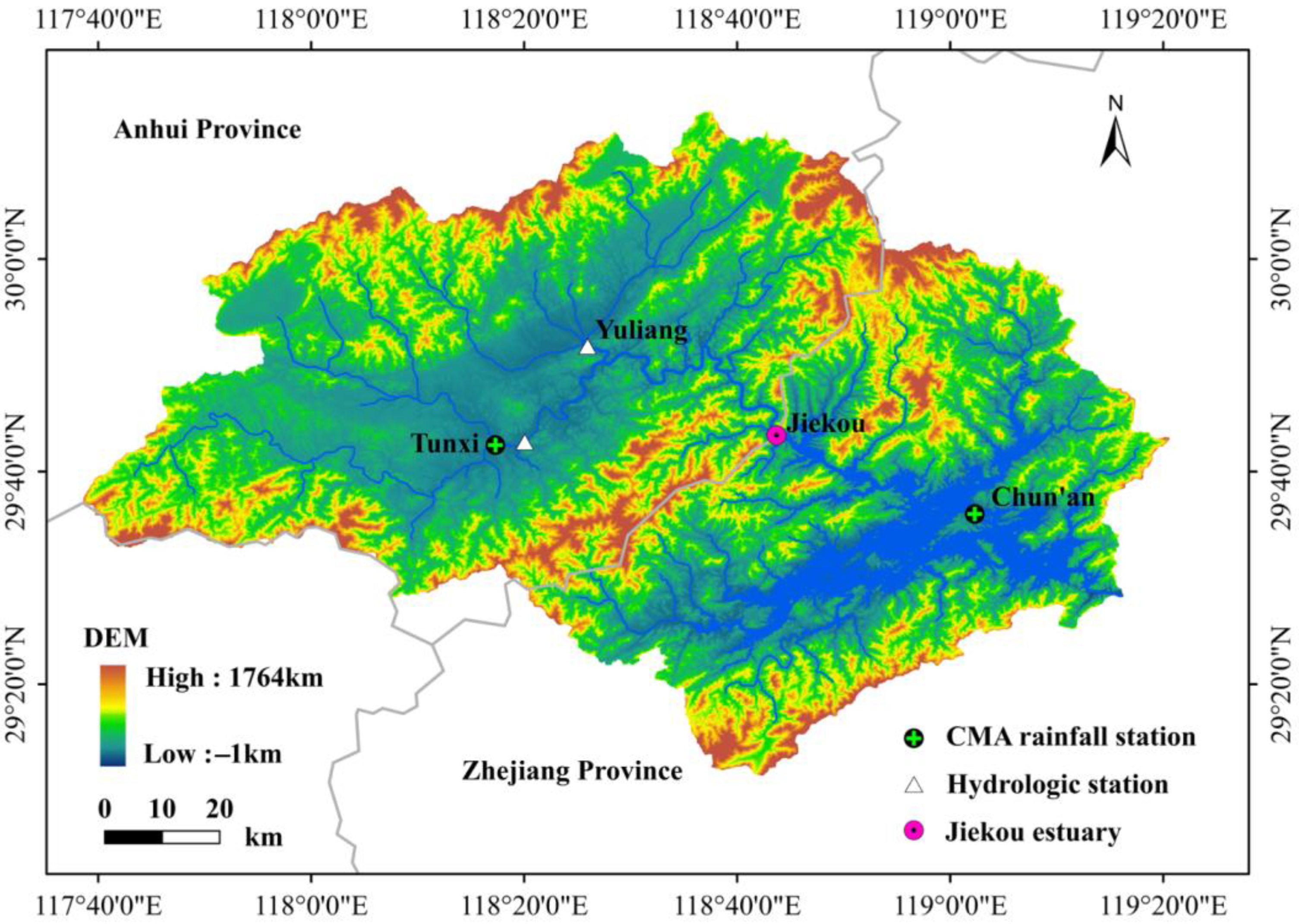
2.1. Study Area
2.2. Data Description
2.2.1. Hydrometeorological Data
2.2.2. Geospatial Data
2.2.3. RCP Data
2.3. Methodology
2.3.1. Climate Change and Land Use/Land Cover Change Scenarios
2.3.2. SWAT Hydrological Model
2.3.3. Sediment Response to Changes of Climate and Land Use/Land Cover
3. Results and Discussion
3.1. Climate Change Analysis under Varying Scenarios
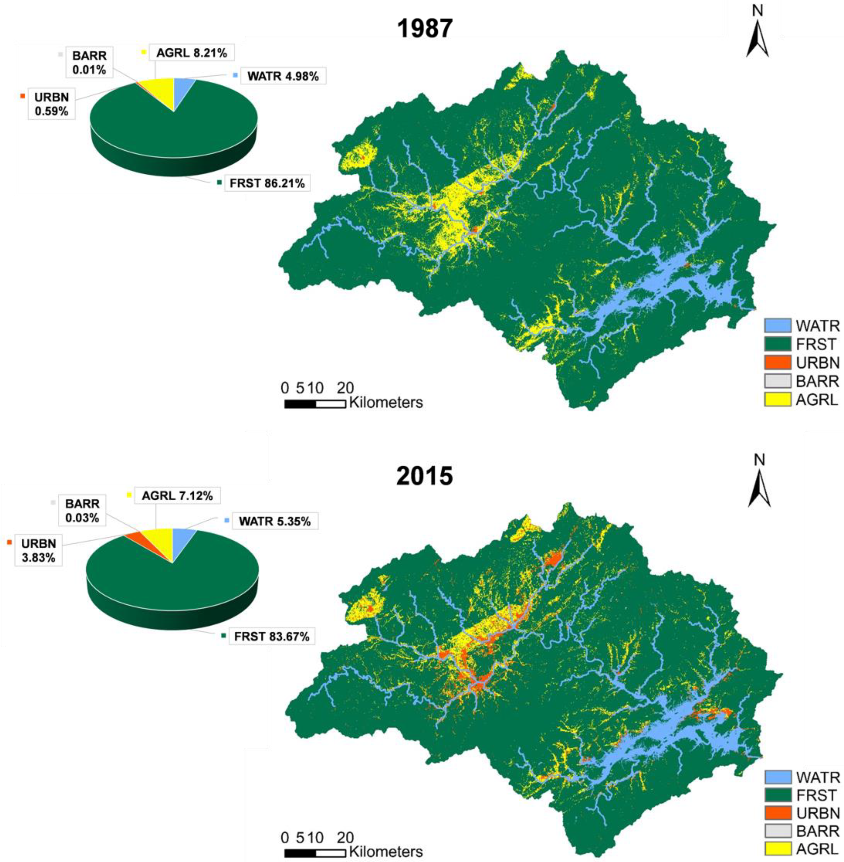
3.2. Land Use/Land Cover Change Analysis under Varying Scenarios
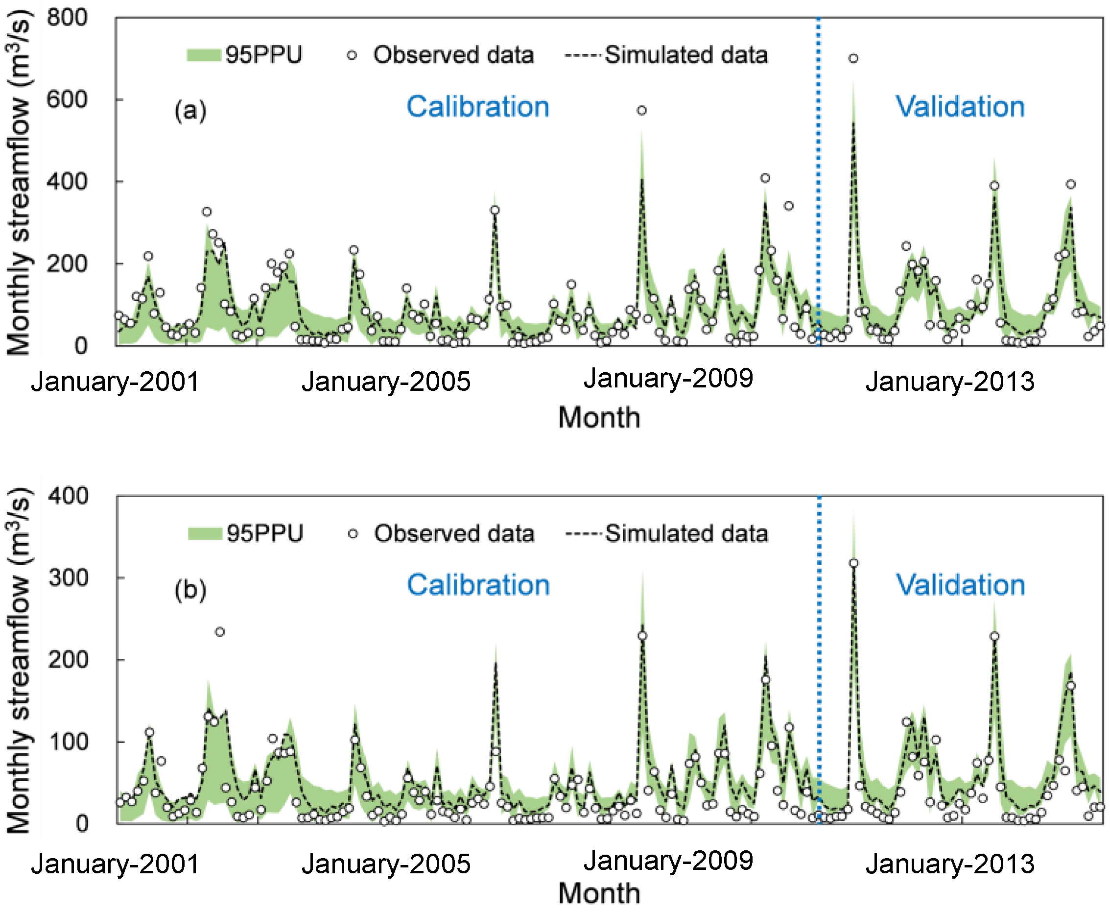
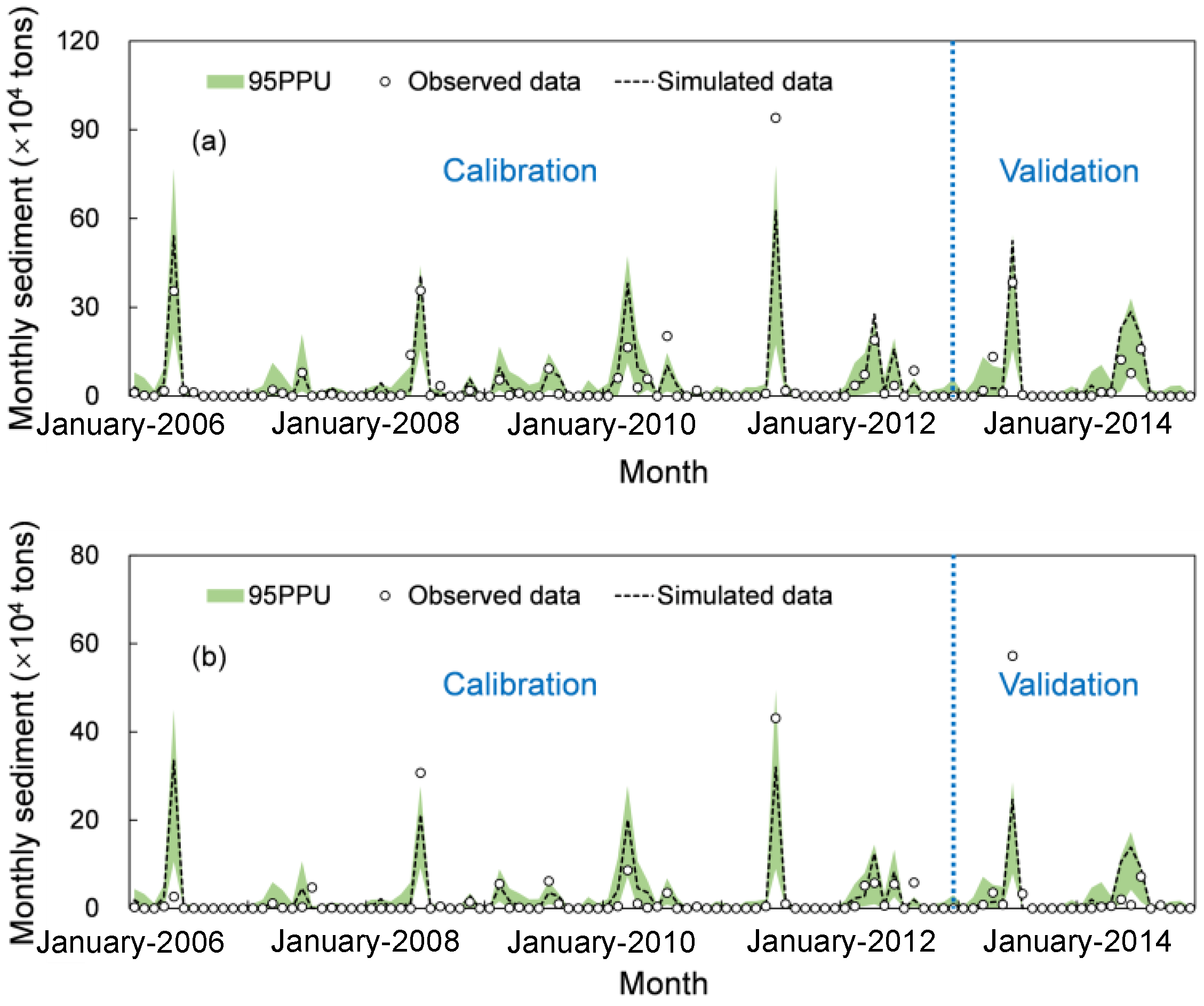
3.3. Results of Sensitivity Analysis and Model Performance Assessment
3.4. Separating Impacts of Climate Variability and Land Use/Land Cover Change on Sediment
3.5. Implication for Water Quality Management of Reservoir/Lake
4. Conclusions
Author Contributions
Funding
Institutional Review Board Statement
Informed Consent Statement
Data Availability Statement
Conflicts of Interest
References
- Van, O.K.; Govers, G.; Desmet, P. Evaluating the effects of changes in landscape structure on soil erosion by water and tillage. Landsc. Ecol. 2000, 15, 577–589. [Google Scholar]
- Zhang, X.C.; Liu, W.Z. Simulating potential response of hydrology, soil erosion, and crop productivity to climate change in Changwu tableland region on the Loess Plateau of China. Agric. For. Meteorol. 2005, 131, 127–142. [Google Scholar] [CrossRef]
- Khoi, D.N.; Suetsugi, T. Impact of climate and land-use changes on hydrological processes and sediment yield—A case study of the Be River catchment, Vietnam. Hydrol. Sci. J. 2014, 59, 1095–1108. [Google Scholar] [CrossRef]
- Li, Z.Y.; Fang, H.Y. Modeling the impact of climate change on watershed discharge and sediment yield in the black soil region, northeastern China. Geomorphology 2017, 293, 255–271. [Google Scholar] [CrossRef]
- Boix-Fayos, C.; Martínez-Mena, M.; Arnau-Rosalén, E.; Calvo-Cases, A.; Castillo, V.; Albaladejo, J. Measuring soil erosion by field plots: Understanding the sources of variation. Earth Sci. Rev. 2006, 78, 267–285. [Google Scholar] [CrossRef]
- Montgomery, D.R.; Brandon, M.T. Topographic controls on erosion rates in tectonically active mountain ranges. Earth Planet. Sci. Lett. 2002, 201, 481–489. [Google Scholar] [CrossRef]
- Wang, H.; Saito, Y.; Zhang, Y.; Bi, N.; Sun, X.; Yang, Z. Recent changes of sediment flux to the western Pacific Ocean from major rivers in East and Southeast Asia. Earth Sci. Rev. 2011, 108, 80–100. [Google Scholar] [CrossRef]
- Langbein, W.B.; Schumm, S.A. Yield of sediment in relation to mean annual precipitation. EOS 1958, 39, 1076–1084. [Google Scholar] [CrossRef] [Green Version]
- Stockwell, J.D.; Doubek, J.P.; Adrian, R.; Anneville, O.; Carey, C.C.; Carvalho, L.; Domis, L.N.D.S.; Dur, G.; Frassl, M.A.; Grossart, H.P.; et al. Storm impacts on phytoplankton community dynamics in lakes. Glob. Chang. Biol. 2020, 26, 2756–2784. [Google Scholar] [CrossRef] [Green Version]
- Shi, Z.H.; Huang, X.D.; Ai, L.; Fang, N.F.; Wu, G.L. Quantitative analysis of factors controlling sediment yield in mountainous watersheds. Geomorphology 2014, 226, 193–201. [Google Scholar] [CrossRef]
- Wang, M.; Hamilton, D.P.; McBridea, C.G.; Abellc, J.M.; Hicksa, B.J. Modelling hydrology and water quality in a mixed land use catchment and eutrophic lake: Effects of nutrient load reductions and climate change. Environ. Modell. Softw. 2018, 109, 114–133. [Google Scholar]
- Lü, X.X.; Ran, L.S.; Liu, S.; Jiang, T.; Zhang, S.R.; Wang, J.J. Sediment loads response to climate change: A preliminary study of eight large Chinese rivers. Int. J. Sediment Res. 2013, 28, 1–14. [Google Scholar] [CrossRef]
- Zabaleta, A.; Meaurio, M.; Ruiz, E.; Antigüedad, I. Simulation climate change impact on runoff and sediment yield in a small watershed in the Basque Country, northern Spain. J. Environ. Qual. 2014, 43, 235–245. [Google Scholar] [CrossRef]
- Imeson, A.C.; Lavee, H. Soil erosion and climate change: The transect approach and the influence of scale. Geomorphology 1998, 23, 219–227. [Google Scholar] [CrossRef]
- Zhao, G.J.; Mu, X.M.; Tian, P.; Wang, F.; Gao, P. The variation trend of streamflow and sediment flux in the middle reaches of Yellow River over the Past 60 years and the influencing Factors. Res. Sci. 2012, 34, 1070–1078. (In Chinese) [Google Scholar]
- Nearing, M.A.; Jetten, V.; Baffaut, C.; Cerdan, O.; Couturier, A.; Hernandez, M.; Le Bissonnaise, Y.; Nicholsa, M.H.; Nunesf, J.P.; Renschlerg, C.S.; et al. Modeling response of soil erosion and runoff to changes in precipitation and cover. Catena 2005, 61, 131–154. [Google Scholar] [CrossRef]
- Jansen, I.M.L.; Painter, R.B. Predicting sediment yield from climate and topography. J. Hydrol. 1974, 21, 371–380. [Google Scholar] [CrossRef]
- Syvitski, J.P.M. The influence of climate on the flux of sediment to the coastal ocean. In Proceedings of the Oceans 2003. Celebrating the Past ... Teaming toward the Future (IEEE Cat. No.03CH37492), San Diego, CA, USA, 22–26 September 2003; Available online: https://ieeexplore.ieee.org/abstract/document/1283423 (accessed on 1 May 2020).
- Phan, D.B.; Wu, C.C.; Hsieh, S.C. Impact of climate change on stream discharge and sediment yield in northern Viet Nam. Water Resour. 2011, 38, 827–836. [Google Scholar] [CrossRef]
- Huang, X. The Effect and Mechanism of Vegetation Cover and Rainfall Change on Runoff and Sediment Yield in Du Watershed, China. Ph.D. Thesis, Huazhong Agricultural University, Wuhan, China, 2019. [Google Scholar]
- Walling, D.E.; Fang, D. Recent trends in the suspended sediment loads of the world’s rivers. Glob. Planet Chang. 2003, 39, 111–126. [Google Scholar] [CrossRef]
- Martin, J.M.; Meybeck, M. Elemental mass-balance of material carried by major world rivers. Mar. Chem. 1979, 7, 173–206. [Google Scholar] [CrossRef]
- Walling, D.E. The Impact of Global Change on Erosion and Sediment Transport by Rivers: Current Progress and Future Challenges; United Nations Educational, Scientific and Cultural Organization: Paris, France, 2009; pp. 1–26. [Google Scholar]
- Montgomery, D.R. Soil erosion and agricultural sustainability. Proc. Natl. Acad. Sci. USA 2007, 104, 13268–13272. [Google Scholar] [CrossRef] [PubMed] [Green Version]
- Sinha, R.K.; Eldho, T.I. Effects of historical and projected land use/cover change on runoff and sediment yield in the Netravati River basin, Western Ghats, India. Environ. Earth Sci. 2018, 77, 111. [Google Scholar] [CrossRef]
- IPCC. Climate change 2014: Synthesis report. In Contribution of Working Groups I, II and III to the Fifth Assessment Report of the Intergovernmental Panel on Climate Change; Pachauri, R.K., Meyer, L.A., Eds.; Core Writing Team, IPCC: Geneva, Switzerland, 2014; p. 151. [Google Scholar]
- IPCC. Global Warming of 1.5 °C. An IPCC Special Report on the Impacts of Global Warming of 1.5 °C above Pre–Industrial Levels and Related Global Greenhouse Gas Emission Pathways, in the Context of Strengthening the Global Response to the Threat of Climate Change, Sustainable Development, and Efforts to Eradicate Poverty; World Meteorological Organization: Geneva, Switzerland, 2018; p. 32. [Google Scholar]
- Vaighan, A.A.; Talebbeydokhti, N.; Bavani, A.M. Assessing the impacts of climate and land use change on streamflow, water quality and suspended sediment in the Kor River Basin, Southwest of Iran. Environ. Earth Sci. 2017, 76, 543. [Google Scholar] [CrossRef]
- Thrasher, B.; Maurer, E.P.; McKellar, C.; Duffy, P.B. Technical note: Bias correcting climate model simulated daily temperature extremes with quantile mapping. Hydrol. Earth Syst. Sci. 2012, 16, 3309–3314. [Google Scholar] [CrossRef] [Green Version]
- Peng, H.; Jia, Y.W.; Qiu, Y.Q.; Niu, C.W.; Ding, X.Y. Assessing climate change impacts on the ecohydrology of the Jinghe River basin in the Loess Plateau, China. Hydrol. Sci. J. 2013, 58, 651–670. [Google Scholar] [CrossRef]
- Zhou, Y.Q.; Jeppesen, E.; Zhang, Y.L.; Shi, K.; Liu, X.H.; Zhu, G.W. Dissolved organic matter fluorescence at wavelength 275/342 nm as a key indicator for detection of point-source contamination in a large Chinese drinking water lake. Chemosphere 2016, 144, 503–509. [Google Scholar] [CrossRef] [PubMed]
- Zhang, Y.L.; Wu, Z.X.; Liu, M.L.; He, J.B.; Shi, K.; Zhou, Y.Q.; Wang, M.Z.; Liu, X.H. Dissolved oxygen stratification and response to thermal structure and long-term climate change in a large and deep subtropical reservoir (Lake Qiandaohu, China). Water Res. 2015, 75, 249–258. [Google Scholar] [CrossRef]
- Da, W.Y.; Zhu, G.W.; Li, Y.X.; Wu, Z.X.; Zheng, W.T.; Lan, J.; Wang, Y.C.; Xu, H.; Zhu, M.Y. High frequent dynamics of water quality and phytoplankton community in inflowing river mouth of Xin’anjiang Reservoir, China. Environ. Sci. 2020, 41, 713–727. [Google Scholar]
- Zheng, Y.N.; Wen, X.; Fang, G.H. Research on climate change and runoff response in Xin’an river basin. J. Water Res. Water Eng. 2015, 26, 106–110. [Google Scholar]
- Pan, Y.; Luo, Y.; Wang, Y.; Zhang, Q.; Zhu, Z. Characteristics of evolution of precipitation and runoff in Xin’an River Basin. Res. Soil Water Conserv. 2018, 25, 121–125. [Google Scholar]
- Li, H.Y.; Wang, Y.C.; Shan, L.; Luo, L.C.; Zhu, G.W.; Xu, H.; Shi, P.C. Effect of rainstorm runoff on total phosphorus load in Xin′anjiang. Res. Environ. Sci. 2022, 35, 887–895. (In Chinese) [Google Scholar]
- Liu, M.; Zhang, Y.L.; Shi, K.; Zhu, G.W.; Wu, Z.X.; Liu, M.L.; Zhang, Y.B. Thermal stratification dynamics in a large and deep subtropical reservoir revealed by high-frequency buoy data. Sci. Total Environ. 2019, 651, 614–624. [Google Scholar] [CrossRef] [PubMed]
- Zhang, Y.L.; Wu, Z.X.; Liu, M.L.; He, J.B.; Shi, K.; Wang, M.Z.; Yu, Z.M. Thermal structure and response to long-term climatic changes in Lake Qiandaohu, a deep subtropical reservoir in China. Limnol. Oceanogr. 2014, 59, 1193–1202. [Google Scholar] [CrossRef]
- Zhu, G.W.; Cheng, X.L.; Wu, Z.X.; Shi, P.C.; Zhu, M.Y.; Xu, H.; Guo, C.X.; Zhao, X.C. Spatio-temporal variation of nutrient concentrations and environmental challenges of Qiandaohu Reservoir, China. Res. Environ. Sci. 2022, 35, 852–863. (In Chinese) [Google Scholar]
- Chen, D.Q.; Li, H.P.; Zhang, W.S.; Pueppke, S.G.; Pang, J.P.; Diao, Y.Q. Spatiotemporal Dynamics of Nitrogen Transport in the Qiandao Lake Basin, a Large Hilly Monsoon Basin of Southeastern China. Water 2020, 12, 1075. [Google Scholar] [CrossRef] [Green Version]
- Zhang, Y.B.; Shi, K.; Zhang, Y.L.; Moreno-Madriñán, M.J.; Zhu, G.W.; Zhou, Y.Q.; Li, Y. River plume monitoring in a deep valley reservoir using HJ-1 A/B images. J. Hydrol. 2020, 587, 125031. [Google Scholar] [CrossRef]
- MWR. Hydrological Data of River Basins in China; Ministry of Water Resources of the People’s Republic of China: Beijing, China, 2015. (In Chinese) [Google Scholar]
- FAO; IIASA; ISRIC; ISSCAS; JRC. Harmonized World Soil Database (Version 1.2); FAO: Rome, Italy; IIASA: Laxenburg, Austria, 2012. [Google Scholar]
- Li, Y.; Zhang, Y.L.; Shi, K.; Zhu, G.W.; Zhou, Y.Q.; Zhang, Y.B.; Guo, Y.L. Monitoring spatiotemporal variations in nutrients in a large drinking water reservoir and their relationships with hydrological and meteorological conditions based on Landsat 8 imagery. Sci. Total Environ. 2017, 599–600, 1705–1717. [Google Scholar] [CrossRef]
- IPCC. Summary for policymakers. In Climate Change 2013: The Physical Science Basis. Contribution of Working Group I to the Fifth Assessment Report of the Intergovernmental Panel on Climate Change; Stocker, T.F., Qin, D., Plattner, G.-K., Tignor, M., Allen, S.K., Boschung, J., Nauels, A., Xia, Y., Bex, V., Midgley, P.M., Eds.; Cambridge University Press: Cambridge, UK; New York, NY, USA, 2013. [Google Scholar]
- Taylor, K. Summarizing multiple aspects of model performance in a single diagram. J. Geophys. Res.-Atmos. 2001, 106, 7183–7192. [Google Scholar] [CrossRef]
- Abbaspour, K.C.; Yang, J.; Maximov, I.; Siber, R.; Bogner, K.; Mieleitner, J.; Zobrist, J.; Srinivasan, R. Modelling hydrology and water quality in the pre-alpine/alpine Thur watershed using SWAT. J. Hydrol. 2007, 333, 413–430. [Google Scholar] [CrossRef]
- Williams, J.R. The EPIC model. In Computer Models of Watershed Hydrology; Singh, V.P., Ed.; Water Resources Publications: Highlands Ranch, CO, USA, 1995; pp. 909–1000. [Google Scholar]
- Abbaspour, K.C.; Johnson, A.; van Genuchten, M.T. Estimating uncertain flow and transport parameters using a sequential uncertainty fitting procedure. Vadose Zone J. 2004, 3, 1340–1352. [Google Scholar] [CrossRef]
- Abbaspour, K.C.; Vejdani, M.; Haghighat, S. SWAT-CUP calibration and uncertainty programs for SWAT. In Proceedings of the Modsim International Congress on Modelling & Simulation Land Water & Environmental Management Integrated Systems for Sustainability, Melbourne, Australia, 3–5 December 2007. [Google Scholar]
- Abbaspour, K.C. SWAT-CUP: SWAT calibration and uncertainty programs—A user manual. Eawag 2015, 6–69, 72–80. [Google Scholar]
- Moriasi, D.N.; Arnold, J.G.; Liew, M.W.V.; Bingner, R.L.; Harmel, R.D.; Veith, T.L. Model evaluation guidelines for systematic quantification of accuracy in watershed simulations. Trans. ASABE 2007, 50, 885–899. [Google Scholar] [CrossRef]
- Santhi, C.; Arnold, J.G.; Williams, J.R.; Dugas, W.A.; Srinivasan, R.; Hauck, L.M. Validation of the SWAT model on a large river basin with point and nonpoint sources, Jawra. J. Am. Water Resour. Assoc. 2010, 37, 1169–1188. [Google Scholar] [CrossRef]
- Moriasi, D.N.; Gitau, M.W.; Pai, N.; Daggupati, P. Hydrologic and water quality model: Performance measures and evaluation criteria. Trans. ASABE 2015, 58, 1763–1785. [Google Scholar]
- Zhang, C.; Huang, Y.X.; Javed, A.; Arhonditsis, G.B. An ensemble modeling framework to study the effects of climate change on the trophic state of shallow reservoirs. Sci. Total Environ. 2019, 697, 134078. [Google Scholar] [CrossRef]
- Guo, Y.X.; Fang, G.H.; Xu, Y.P.; Tian, X.; Xie, J.K. Identifying how future climate and land use/land cover changes impact streamflow in Xinanjiang Basin, East China. Sci. Total Environ. 2020, 710, 136275. [Google Scholar] [CrossRef]
- Mann, H.B. Nonparametric tests against trend. Econometrica 1945, 13, 245–259. [Google Scholar] [CrossRef]
- Kendall, M.G. Rank Correlation Methods, 4th ed.; Charles Griffin: London, UK, 1975. [Google Scholar]
- Zhang, Y.L.; Shi, K.; Zhou, Y.Q.; Liu, X.H.; Qin, B.Q. Monitoring the river plume induced by heavy rainfall events in large, shallow, Lake Taihu using MODIS 250 m imagery. Remote Sens. Environ. 2016, 173, 109–121. [Google Scholar] [CrossRef]
- Yang, Z.; Zhang, M.; Shi, X.L.; Kong, F.X.; Ma, R.H.; Yu, Y. Nutrient reduction magnifies the impact of extreme weather on cyanobacterial bloom formation in large shallow Lake Taihu (China). Water Res. 2016, 103, 302–310. [Google Scholar] [CrossRef]


| Scenario | Simulation Time | Land Use/Cover | Climate | Description |
|---|---|---|---|---|
| 1973–2005 | LULC1987 | History | Baseline | |
| 2068–2100 | LULC1987 | RCP2.6 | With a stringent mitigation scenario and no land use/land cover change | |
| 2068–2100 | LULC1987 | RCP4.5 | With an intermediate scenario and no land use/land cover change | |
| 2068–2100 | LULC1987 | RCP8.5 | With a very high greenhouse gas emission scenario and no land use/land cover change | |
| 1973–2005 | LULC2015 | History | With a land use/land cover change and no climate change | |
| 2068–2100 | LULC2015 | RCP2.6 | With land use/land cover change and a stringent mitigation scenario | |
| 2068–2100 | LULC2015 | RCP4.5 | With land use/land cover change and intermediate scenario | |
| 2068–2100 | LULC2015 | RCP8.5 | With land use/land cover change and a very high greenhouse gas emission scenario |
| Parameter | Definition | Sensitivity Analysis | Calibration | |||
|---|---|---|---|---|---|---|
| t-Statistics | p-Value | Min | Max | Optimal | ||
| Streamflow | ||||||
| CN2 * | SCS runoff curve number for moisture condition II | −35.47 | 0.00 | −0.5 | 0.5 | 0.047 |
| CH_K2 | Effective hydraulic conductivity in main channel alluvium (mm/h) | −2.64 | 0.01 | −0.01 | 500 | 378.873 |
| SOL_Z * | Depth to bottom of first soil layer (mm) | 2.57 | 0.01 | −0.5 | 0.5 | 0.148 |
| SURLAG | Surface runoff lag time (days) | −0.96 | 0.34 | 0.05 | 24 | 17.324 |
| ESCO | Soil evaporation compensation factor | 0.64 | 0.53 | 0 | 1 | 0.347 |
| GW_DELAY | Groundwater delay (days) | 0.58 | 0.56 | 30 | 450 | 62.025 |
| GWQMN | Threshold depth of water in the shallow aquifer for return flow to occur (mm H2O) | −0.50 | 0.62 | 0 | 5000 | 46.250 |
| SOL_K * | Saturated hydraulic conductivity of first soil layer (mm/h) | 0.39 | 0.70 | −0.8 | 0.8 | 0.638 |
| CANMX | Maximum canopy storage (mm H2O) | 0.29 | 0.77 | 0 | 100 | 90.425 |
| SOL_AWC * | Available water capacity of first soil layer (mm/mm) | 0.19 | 0.85 | −0.5 | 0.5 | −0.251 |
| ALPHA_BF | Baseflow alpha factor (days) | −0.14 | 0.89 | 0 | 1 | 0.768 |
| CH_N2 | Manning’s “n” value for the main channel | −0.01 | 0.99 | −0.01 | 0.3 | 0.295 |
| Sediment | ||||||
| USLE_P | USLE equation support practice factor | −39.88 | 0.00 | 0 | 1 | 0.020 |
| SLSUBBSN * | Average slope length (m) | −12.38 | 0.00 | −0.9 | 0.9 | −0.498 |
| BIOMIX | Biological mixing efficiency | −6.52 | 0.00 | 0 | 1 | 0.051 |
| SPEXP | Exponent parameter for calculating sediment re-entrained in channel sediment routing | 1.07 | 0.29 | 1 | 1.5 | 1.429 |
| SPCON | Linear parameter for calculating the maximum amount of sediment that can be re-entrained during channel sediment routing | 0.77 | 0.44 | 0.0001 | 0.01 | 0.006 |
| Variables | Stations | Periods | Monthly Average | Classes | |||
|---|---|---|---|---|---|---|---|
| Observed | Simulated | ||||||
| Streamflow (m3/s) | Tunxi | Calibration | 78.3 | 66.6 | 0.83 | 0.85 | Very good/Good |
| Validation | 108.9 | 114.7 | 0.89 | 0.90 | Very good/Good | ||
| Yuliang | Calibration | 35.7 | 38.8 | 0.64 | 0.69 | Satisfactory/Satisfactory | |
| Validation | 46.2 | 67.7 | 0.73 | 0.88 | Good/Good | ||
| Sediment (thousand tons) | Tunxi | Calibration | 38.9 | 43.3 | 0.70 | 0.71 | Good/Satisfactory |
| Validation | 38.1 | 54.0 | 0.74 | 0.81 | Good/Good | ||
| Yuliang | Calibration | 16.0 | 24.1 | 0.60 | 0.62 | Satisfactory/Satisfactory | |
| Validation | 28.0 | 29.8 | 0.47 | 0.55 | Satisfactory/Satisfactory | ||
| Scenarios | |||||
|---|---|---|---|---|---|
| RCP2.6 | 26.85 | 0.53 | 27.39 | 98.05 | 1.95 |
| RCP4.5 | 20.07 | 0.53 | 20.60 | 97.45 | 2.55 |
| RCP8.5 | 21.87 | 0.60 | 22.47 | 97.33 | 2.67 |
Publisher’s Note: MDPI stays neutral with regard to jurisdictional claims in published maps and institutional affiliations. |
© 2022 by the authors. Licensee MDPI, Basel, Switzerland. This article is an open access article distributed under the terms and conditions of the Creative Commons Attribution (CC BY) license (https://creativecommons.org/licenses/by/4.0/).
Share and Cite
Li, H.; Yu, C.; Qin, B.; Li, Y.; Jin, J.; Luo, L.; Wu, Z.; Shi, K.; Zhu, G. Modeling the Effects of Climate Change and Land Use/Land Cover Change on Sediment Yield in a Large Reservoir Basin in the East Asian Monsoonal Region. Water 2022, 14, 2346. https://doi.org/10.3390/w14152346
Li H, Yu C, Qin B, Li Y, Jin J, Luo L, Wu Z, Shi K, Zhu G. Modeling the Effects of Climate Change and Land Use/Land Cover Change on Sediment Yield in a Large Reservoir Basin in the East Asian Monsoonal Region. Water. 2022; 14(15):2346. https://doi.org/10.3390/w14152346
Chicago/Turabian StyleLi, Huiyun, Chuanguan Yu, Boqiang Qin, Yuan Li, Junliang Jin, Liancong Luo, Zhixu Wu, Kun Shi, and Guangwei Zhu. 2022. "Modeling the Effects of Climate Change and Land Use/Land Cover Change on Sediment Yield in a Large Reservoir Basin in the East Asian Monsoonal Region" Water 14, no. 15: 2346. https://doi.org/10.3390/w14152346