Visualization Assisted Approach to Anomaly and Attack Detection in Water Treatment Systems

Abstract

The specificity of the water treatment field, associated with water transmission, distribution and accounting, as well as the need to use automation and intelligent tools for various information solutions and security tools, have resulted in the development of integrated approaches and practical solutions regarding various aspects of the functioning of such systems. The research problem lies in the insecurity of water treatment systems and their susceptibility to malicious influences from the side of potential intruders trying to compromise the functioning. To obtain initial data needed for assessing the states of a water treatment system, the authors have developed a case study presenting a combination of a physical model and a software simulator. The methodology proposed in the article includes combining methods of machine learning and visual data analysis to improve the detection of attacks and anomalies in water treatment systems. The selection of the methods and tuning of their modes and parameters made it possible to build a mechanism for efficient detection of attacks in data from sensors with accuracy values above 0.95 for each class of attack and mixed data. In addition, Change_Measure metric parameters were selected to ensure the detection of attacks and anomalies by using visual data analysis. The combined method allows identifying points when the functioning of the system changes, which could be used as a trigger to start resource-intensive procedures of manual and/or machine-assisted checking of the system state on the basis of the available machine learning models that involve processing big data arrays.

1. Introduction

Today, industrial Internet of Things systems and wireless sensor networks are becoming more widespread. Such systems are used to monitor people, environments, technical devices and other physical objects. The major threat for such monitoring systems is functioning in an unreliable environment, assuming the presence of malicious attacking activity. These threats could lead to a compromise of the system as a whole, its devices and services [1]. The system compromise may result in catastrophic consequences, such as disruption of the system functioning, distortion of the collected data or significant delays in their transmission. These impacts can disrupt the processes of notifying the system operator about failures and security incidents, which can lead to hazardous effects. In the context of water treatment systems, the impacts on water level sensors can cause flooding of the reservoir or its shallowing, resulting in violations of the water supply processes involving end consumers. Therefore, there is a need to develop effective models and techniques to identify malicious actions on sensors and the system as a whole. Rapid detection of security incidents will allow an operator to respond to them in a timely manner and avoid or at least minimize negative consequences.

Generally, the work presents an approach for attack and anomaly detection that utilizes both machine learning and visualization techniques. Along with the classical machine learning analysis models, it is proposed to use a metric that characterizes the changes in the system for visual exploration of system parameters. This solution also supports validation of the constructed machine learning classifiers by means of the visual analysis and exploration of the system parameters as well as the system state to check the effectiveness of these analysis models. Such ongoing validation allows signaling the need to reconfigure the functioning classifiers due to the possible and expected natural evolution of the target system. The proposed detection mechanisms could be used in real-time and near-real-time modes, thus allowing the generation of alerts of security incidents with acceptable detection quality for a given time period.

Thus, the novelty of the proposed approach consists of the combination of the machine learning and visualization techniques that are used in conjunction to monitor both the system state and efficiency of the analysis models. The developed visualization serves as an express assessment of the system state. It could be made to obtain more detailed manual and/or machine-assisted assessments of the system. In addition, the applied visualization contributes to the reconfiguration and improvement of the machine learning classifiers, allowing one to take into account even relatively small changes in the behavior of the target system.

Due to the limitations of the available equipment, a specific test bed for the water treatment system was developed. It was built on the principles of the full-scale and simulation modeling of the analyzed industrial process. The full-scale model was developed using Arduino microcontrollers, physical sensors and actuators, including sensors of water level, pressure and water flow, as well as electric valves and a water pump. It is enriched by a set of simulation rules that generate vectors of sensor readings and the state of actuators based on some numerical features of the implemented full-scale model. Combining the full-scale and simulation models made it possible to generate data sets that characterize the normal behavior of the system and several classes of attacks on its sensors. In addition, one should note that, on the physical implementation, we calculated a few important parameters of the modeled processes (including measurements of the time of emptying/filling of tanks and the rate of change of sensor readings). Then, we used the values of these parameters straightforwardly within the software simulator, which more fully describes the analyzed water treatment processes. This explains why both the full-scale model and the software simulator were really needed. Note that the developed machine learning and visualization models were built using the data collected from the developed test bed.

Thus, the contributions of the paper consist of

• An approach combining machine learning and visualization models to monitor the state of a water treatment system;
• An application of the metric that characterizes the measure of system change to monitor and analyze the state of the system visually;
• A water treatment test bed that is developed on the principles of the full-scale and simulation modeling of the technological process.

The rest of the article is organized as follows. Section 2 represents the state-of-the-art. Section 3 discusses the whole visualization-assisted approach to anomaly and attack detection, while Section 3 details the visualization-driven explanation and analysis component. Section 4 presents a case study and the developed test bed. Section 5 contains the experimental study and discussion, while Section 6 concludes the article.

2. Related Works

Currently, the security of the Internet of Things systems and wireless sensor networks has been the subject of a series of works. Some of them deal with aspects related to attacks on the routing protocol. For example, Rehman et al. suggested several ways to detect Sinkhole attacks, i.e., sophisticated routing effects [2]. In contrast to existing ones, the specificity of this article is that it concerns elements of attack detection by identifying correlations between sensor readings without considering direct malicious actions on the network protocol level and/or other physical and software parts.

The issues of ensuring and assessing the security of Internet of Things systems, robotic complexes and wireless sensor networks, including studies of the impact on device sensors, are becoming increasingly relevant [1]. By influencing the system by exploiting one or a few sensors, as the point of the application, the attacker is able to compromise a sensor and devices integrated with it or located near it. In addition, the attacker can interfere with the data transmitted, processed and stored on the network devices and the information services provided. An attack on a sensor can be an element of a complex influence that can lead to various short-term or fatal disruptions in the functioning of the entire system and cause its inoperability. One of the ways to increase the security of such systems is the timely detection of malicious influences and obtaining additional information on them, including the class and source of the attack.

In most of the analyzed literature sources, the detection of attacks and anomalies in Internet of Things systems is performed using various intelligent data analysis methods [1,3,4]. At the same time, the extraction of specific features, the construction of feature spaces, and the appointment of certain learning models, for the most part, are determined by the specific formulation of the problem and its limitations. In particular, the availability or absence of satellite communications in the network determine the short-term loss of connection accompanying this type of connection, especially due to the continuous movement of satellites in the orbit and the possible movement of ground devices of the network [5]. Depending on the structure and composition of the system, such losses should be separated from targeted actions of the attacker, for example, ones aimed at noising the GPS channel.

Wang et al. [3] proposed a way to detect attacks on sensors in a wireless sensor network by introducing a virtual sensor and using a sensor’s fault model to establish inconsistencies between the readings of this sensor and other ones to be considered as attacks. Shin et al. analyzed data from sensors of intelligent vehicle models to detect anomalies by using deep learning methods [1]. It is based on quantitative measurements of the readings of eight physical sensors of the car model, and the difference in the values of the sensor readings from the expected values is estimated. In the study, six particular classes of attacks and normal data are used. Each of them represents an attack on one or two of the available sensors. The conducted experiments made it possible to compute the indicators of accuracy and correctness, as well as to determines the training methods that grant the best outcome.

In [5], by using the example of unmanned ground vehicles, some attacks on sensors are detected in conditions of possible transient faults. To distinguish between attacks and transient faults, a static model of the faults (faulty model) is built for each sensor, including the interval of its allowable values and the maximum allowable frequency of its faults. The attacks are detected on the basis of these models by pairwise comparisons of the readings of various sensors. In the process of machine learning, the most appropriate fault model is selected from the available models.

Currently, a fairly large number of studies are being conducted on digital water metering and related directions, including issues of water consumption, long medium and short-term prediction of such consumption, resource planning, explanation of user behavior, characteristics of water consumption and detection of leaks by using machine learning and data analysis methods [6].

Racity et al. proposed a mechanism for monitoring water quality, including checking for contamination and other characteristics of water [7]. At the same time, a particular requirement is established to achieve a high quality of detection in conditions of possible inaccuracies and the absence of some feature’s values. Based on the application of water clustering methods, Raciti et al. built a mechanism for detecting pollution with certain values of the detection quality.

In [8], the correlation between the properties of pollution of terrestrial natural water bodies and geographic characteristics of the location, such as latitude, longitude and height, is considered. In that work, a number of polluting factors (contaminating factors, e.g., water temperature, turbidity, acidity, the presence of oxygen in water, chlorides, etc.) are identified, and they are used to predict specific pollution based on physical parameters. The data analysis is performed using machine learning methods, namely four regression models. A peculiarity of this work is the manual collection and physical and chemical analysis of water to obtain a set of data on the pollution characteristics in various areas of the region under consideration, followed by the use of particular methods of data mining.

Artificial intelligence methods are also used to determine the quality of water. In particular, Naloufi et al. proposed a method for predicting the concentration of Escherichia coli bacteria in water bodies without involving complex specific laboratory procedures, which are time-consuming and technically complex and would require higher financial costs [9]. Specifically, Naloufi et al. were able to build a machine learning model that, based on 10 simple physical, chemical and weather characteristics that can be easily measured, generates concentration predictions for a given bacterial species by using basic machine learning methods such as SVM, KNN, DT and others. In addition, the authors note the possibility of automating monitoring and elucidating water pollution using wireless sensor networks, such as LPWAN, which allow nodes to operate autonomously for a long time without replenishing energy resources.

An anomaly detection process may significantly benefit from the application of the visualization techniques as they allow presenting data in clear and easily perceived form. Numerous research papers are devoted to the design of the visualization techniques applicable to the anomaly detection problem [10,11]. For example, Shi et al. [12] reviewed 150 papers and outlined four main application domains for visualization-driven detection of abnormal entity behavior: network communication, social interactions, financial transactions, and travel data. In [13], the authors studied different visualization techniques designed specifically for revealing anomalous activity in the network traffic. However, there are only a few works in the field of visualization-assisted anomaly detection in data from physical sensors. This fact could be explained by the fact that all technological processes are formalized, and any deviation from the predefined process could be detected on the basis of a set of established rules, and the exception is constituted by the problem of equipment failure forecasting, where different machine learning and visualization-driven approaches have been proposed [14].

Commercial SCADA systems [15,16] and commercial solutions for anomaly detection in industrial IoT systems [17] mostly utilize standard visualization techniques such as timelines, gauges or mnemonic object diagrams for graphical representation and analysis of system parameters. The problem arises when analyzing and monitoring the system behavior where an analyst or operator needs to review tens of parameters, and the application of advanced visualization techniques could increase the efficiency of their work. Only a few visual analytics solutions aimed to assist in the monitoring of complex object behavior and anomaly detection are suggested.

Janetzko et al. [18] explored the capabilities of pixel based techniques with different layouts and line charts to detect patterns and anomalies in energy consumption. In [19], the authors adopted matrix-based and RadViz visualizations to analyze anomalies in heating, ventilation and conditioning data.

In [20], the authors applied another multidimensional data projection technique, namely multidimensional scaling, to analyze streaming data from multiple sensors. To be able to apply it, the authors evaluated the pairwise similarity in data streams from sensors and used it to map sensors on the plane. Such projection allowed the authors to represent sensors’ functioning as a trajectory of points on the plane, and anomalies in their behavior could be detected as anomalies in their trajectories.

In [21], the authors proposed an interactive visual analytics system for equipment line monitoring that supports not only smart parameter monitoring but also machine learning model inspection and updates. The latter is achieved by evaluating the characteristics of the training set and current data. To visualize streams of sensor data, the authors use either line charts with the time axis or pixel-based visualization to cope with large volumes of data.

Let us note the main peculiarities that distinguish this work from the analyzed existing results in the field:

• Focus on the subject area of water treatment. In particular, when defining the classes of attacks, the authors considered the nature of the viscosity and fluidity of water, which determines some inertia and often a gradual change in the accumulation and transfer of water, and as a result, sensor readings in the generated time sequences.
• Building and configuring a set of classifiers as attack and anomaly detection tools based on machine learning methods specific to the problem being solved and the list of critical attacks generated.
• Application of the visual models as means of visual exploration of the system parameters, and monitoring of the system state. The peculiarity of this component lies in the computation and visualization of the metric that characterizes the changes in the system at some given moment of time.
• Combination of the proposed visual analysis and machine learning methods, and presentation of the visual-based express evaluation of the system to make decisions on more detailed manual and/or machine-assisted checking of the system state, firstly, and visual validation of the constructed machine learning classifiers by means of visual analysis and exploration of the system parameters as well as the system state to check the effectiveness of these classifiers, secondly.

3. Visualization-Assisted Approach to Anomaly and Attack Detection

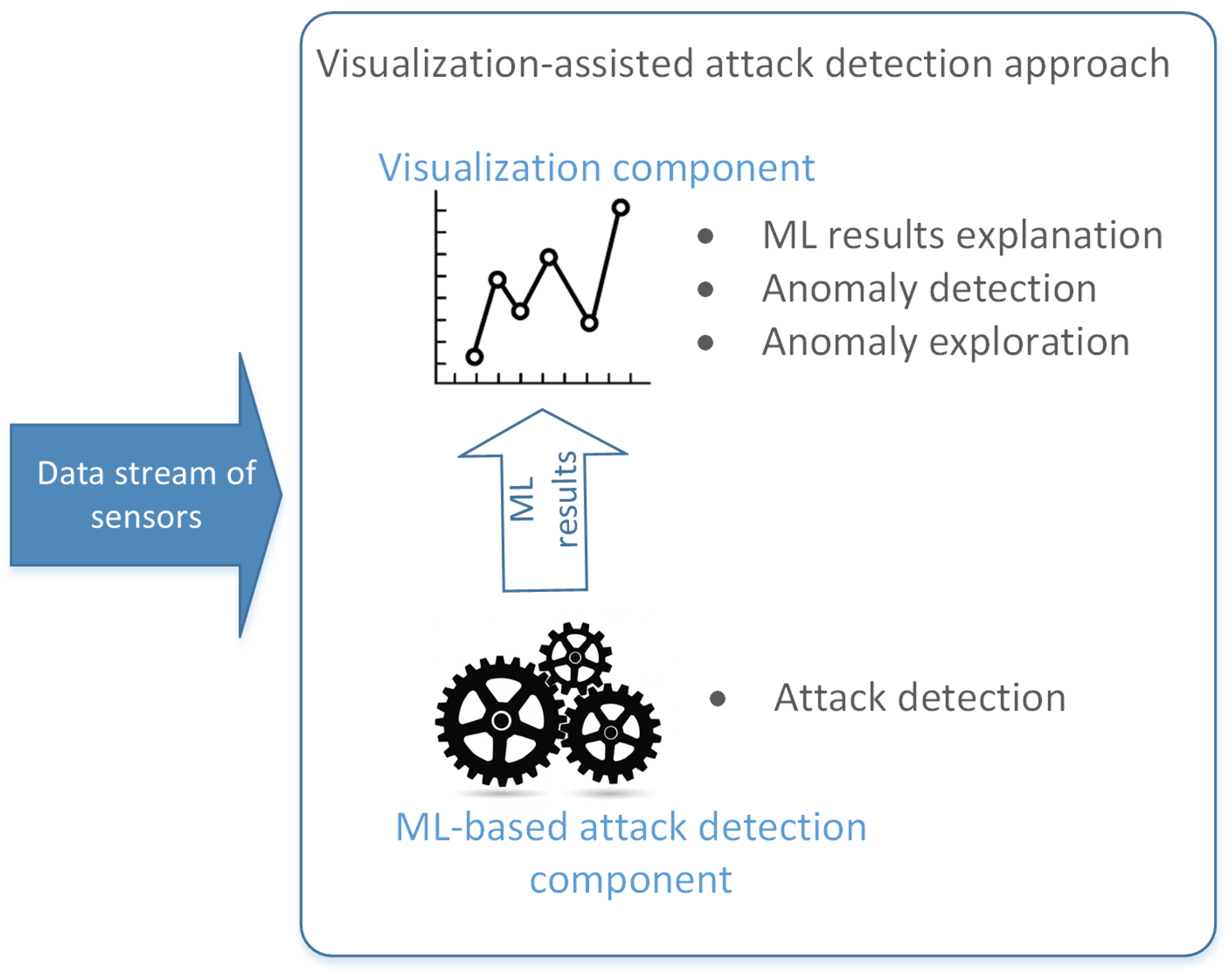
The suggested approach to anomaly and attack detection in the water treatment system consists of the two key connected components:

• Attack detection component based on supervised machine learning;
• Sensor data visualization component.

The scheme of the proposed approach is presented in Figure 1.

The attack detection component consists of n binary classifiers that are trained to detect n different classes of the attacks, and one generalized multi-class classifier targeted to detect one of the n specific attacks. The current implementation of the component detects five different classes of the attacks but could be extended to detect novel ones. The following seven supervised machine learning methods were selected as possible candidates for detecting each class of attack and serving as basis for a generalized multi-class classifier: AdaBoostClassifier, RandomForestClassifier, Bayesian classifier, LogisticRegression, Linear SVM classifier, Decision Trees, and RidgeClassifier. A series of experiments on the test data sets made it possible to determine the most effective machine learning model as well as its parameters. The efficiency assessment was conducted using two quality metrics: accuracy and f1-score. Section 5 discusses the experiment settings as well their results in detail.

The visualization component supports the visual exploration of the system parameters and monitoring of the system state. The distinctive feature of this component is the calculation and visualization of the metric that characterizes the number of changes in the system at the given moment of time. This metric was firstly introduced in [10] and considers a set of selected attributes that are used to evaluate how the system state changes over time. The calculation of the integral metric is presented in Section 3 in detail. To visualize the values of this metric, the line plot with time axis is used. The selected visualization model is simple but intuitively clear to the operator. It provides a natural perception of the situation and allows unambiguous identification of changes in the system that could correspond to the anomalies or attacks in the system behavior.

Visualization-Driven Explanation and Analysis Component

When designing the visualization of data streams from sensors, the authors kept in mind following challenges identified in [22]

• Necessity to combine streaming data from diverse sources to support analysis;
• Support for understanding changes that could be expressed in many forms, starting from changes in parameters’ values between previous and current ones and finishing with deviations in system behavior as a whole;
• Dynamic nature of data, which are constantly changing and evolving in time.

In [19], the authors suggested representing a state of the system that is defined by a set of sensors as a point in a multidimensional space, and then the functioning of this system could be considered as a trajectory in this space. Such representation allows addressing the first challenge relating to the necessity to combine streaming data from multiple sources. Moreover, in [19], it was shown that mapping a system’s trajectory in multidimensional space to the plane enables revealing system behavior patterns as well as anomalies. Different states of the system are characterized by different graphical patterns that vary in point density and scatter. In [23], the authors evaluated different metrics that could be used to assess the similarity of the points distribution on the plane in order to detect structural similarity, and they showed that Delaunay triangulation could be used to detect typical patterns as well as outliers when evaluating projections produced by data reduction techniques. Anomalous bursts in the system’s parameters result in larger values of the total square of the triangles obtained by Delaunay triangulation, while smaller values of the total triangles’ square correspond to smoother changes in the system’s behavior. The latter enabled the authors to define a novel $Change\_Measure$ metric that characterizes the amount of system change and use it as an integral metric to monitor the state of the system [10].

The integral $Change\_Measure$ metric is a core metric of the developed visualization system, and its usage addresses the second challenge identified in [22], enabling an analysis of changes in the whole system as well as changes between previous and current parameters’ values. The metric is calculated for some given moment of time t and considers n subsequent data points in multidimensional space. The algorithm for calculation $Change\_Measure(t,n)$ metric is given in Algorithm 1.

Algorithm 1: Integral $Change\_Measure(t,n)$ metric calculation

Input: n—size of sliding window for sampling a sequence of points, t—moment of time S—a set of m-dimensional data points ordered in time and equipped with timestamps Output: $Change\_Measure(t,n)$ 1: apply data reduction technique PCA to the normalized set S 2: form a subset $S^{\prime }(t,n)$ by selecting n sequential points from the S set that precedes a point with timestamp t 3: construct a Delaunay triangulation $DP\left(S^{\prime }(t,n)\right)$ for a set $S^{\prime }(t,n)$. 4: calculate $Change\_Measure(t,n)$ as a total area of obtained triangles of $DP\left(S^{\prime }(t,n)\right)$. 5: return$Change\_Measure(t,n)$

Currently, to reduce the data dimension, PCA is chosen as it allows revealing the deviations in a systems’ behavior more clearly than other techniques [23]. The size of sliding window n is a customizable parameter and could be changed to enable better anomaly detection. Varying the window size, it is possible to control the impact of previous values on the current one.

The values of the $Change\_Measure(t,n)$ form a one-dimensional time series, and for this reason, it is natural to use the timeline to visualize it. To correlate system behavior with the results of the ML-based attack detection component and to highlight the periods when the system is under attack, the authors use a background color for the plot. The white background corresponds to the normal mode of system functioning, while the color background indicates that the ML-based attack detection component has detected an attack.

In order to enhance the detection of visual signs of an anomaly in the system operation, the authors also propose performing post-processing of the obtained values of the $Change\_Measure(t,n)$ metric. It is possible to apply sliding mean and median filters with a specified width of the filtering window.

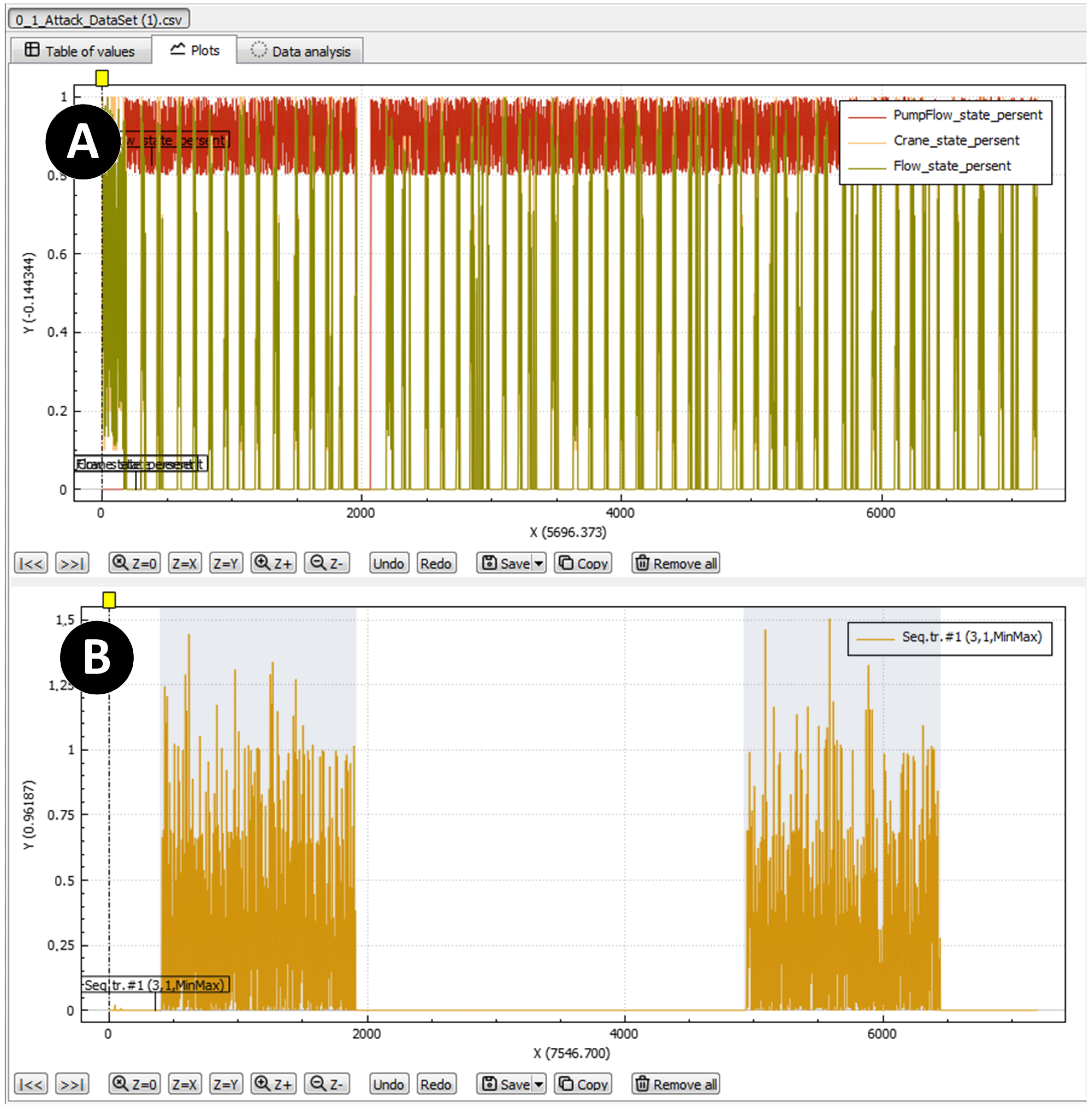
It should also be noted that the suggested visualization provides an overview of the system functioning, which is why it has to be supplemented by a set of timelines showing each parameter separately. Figure 2 shows the graphical interface of the visualization component, which consists of two main views: view A is used to represent values of the system parameters, and view B is used to visualize the integral metric $Change\_Measure(t,n)$. These two views are synchronized, and the operator may select different time intervals to analyze and explore data. They could also choose different parameters to visualize and adjust the graphical properties of the plots. Similarly, the operator could adjust the calculation of the integral score metric by manipulating the sliding window size and applying different filters to smooth the values of $Change\_Measure(t,n)$.

4. Water Treatment Case Study

A case study modeling water treatment with the use of some available physical and electronic components was constructed. In addition, we developed a software tool expanding its business logic and simulating the system processes. This combined scheme allowed us to measure sensor readings directly and multiply and scale them by means of the simulator [24].

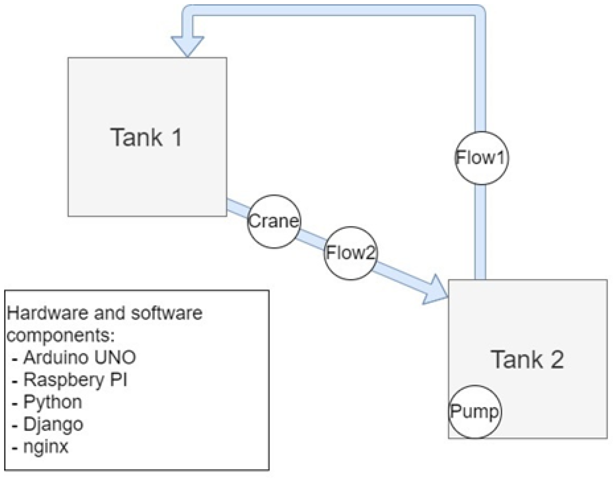
The scheme of the case study used in the work is exposed in Figure 3. The system contains two tanks. One tank is higher than the other (the top one is labeled as the first one and the bottom one as the second tank). Due to the influence of gravity, the water starts flowing from the first tank into the second one. The gate of the water treatment system imitates a controlled tap (electric crane) installed between the tanks. The tap closes when the second tank is full, and then the pump turns on and pumps the water back into the first tank. It simulates the process of lowering the water level on one side of the crane and rising on the other. To measure the water level in the tanks, water level sensors are installed. Each tank has three water level sensors and one sensor measuring the fullness degree. To measure the amount of water pumped between the tanks, in addition to the tap, a water flow sensor is installed. The hardware of the prototype is expressed by an Arduino UNO controller designed to read sensor readings and Raspberry PI for processing them and organizing functions to monitor the system’s status. The software part includes a Web server built using the Python programming language, Django framework and ngnix libraries. This server is used to monitor the readings of sensors and states of the system actuators by a human operator.

It should be noted that the developed prototype is a physically closed system. This is intended to facilitate its continued automatic operation in laboratory conditions and model target water treatment and dam systems closer to their reality. The tanks model water bodies on either side of the gate (shutter). When the gate is opened, the water level decreases on one side and increases on the other (water flow from tank 1 to tank 2). When the valve is closed, the water level decreases on one side (water goes further downstream), and on the other side, it increases (pumping from tank 2 back to 1). The pump was introduced in the model mainly to provide long enough working scenarios of the system.

The developed simulator allowed us to generate a large number of possible states, which made it possible to speed up the modeling and testing of a variety of attacks, i.e., it is able to simulate attacks of several classes and form sets of various particular system states. For example, if it is necessary to generate a data set containing several hours of system operation, it is necessary to run the system model for the required time and constantly simulate attacks, and when simulating, this process is automated and takes less time.

The constructed simulator works as follows: the initial state of the sensors and actuators of the system is set, then the actions occurring in the system are simulated by changing the readings of some sensors over a certain time (for example, half a second), and the related readings of other ones are adjusted. The simulator based on a short recording of sensor readings makes it possible to introduce small deviations into it, concatenating and mixing with other data, to generate longer logs at the output that simulate the operation of the system, thereby increasing the amount of data suitable for experiments.

The formation of mixed data, including data of normal behavior and data about an attack of a certain class, is performed by modeling attack data and superimposing it on records of the normal functioning of the system. After that, these data are written to the output file and meta-information about it is formed. The specific values of the parameters, the time it takes for the tanks to be empty and the readings of specific sensors to change were obtained empirically using a full-scale model. Thus, using the simulation model, it became possible to set any initial state of the system, simulate one of the possible attacks and obtain the required set of system state records within a certain time interval.

The simulation algorithm is shown in Figure 4 as an activity diagram. The data set is in the form of *.csv file, which contains records of sensor readings and states of actuators at certain points in time. Each time moment of the system operation corresponds to a row of value records separated by a syntactic separator. Here, the time interval between records is fixed and is equal to half a second.

During the simulation, seven data sets both with and without attacks were recorded. The constructed data sets include: data containing only normal states of the system; five sets containing normal states together with attack situations of each class, respectively; a set containing all classes of attacks at once and the normal state of the system. The duration of each data set is 1 h (7200 samples). The number of attacks in each file fills 25 min in total, divided into two attacking blocks (i.e., 12.5 min of attacks in each of the two blocks). That is, after an hour of the system’s operation, the attack was modeled on it twice for 12.5 min each. In the data set containing all five attack classes, the time of each attack is the same and is 10 min.

Table 1. Fields of the generated data sets.

No	Data Field Name (Features)	Description
1	id_record_inc	- unique record identifier. It represents a field of Integer data type and is incremented by 1 when a new line is written to the output file. It is greater than zero always
2	watLevel_R1_3_bool	- readings of the upper water level sensor from the first tank. It represents a Boolean type variable. If this variable equals 0, the sensor does not work (the water level is below the sensor). If it is 1, the sensor works
3	watLevel_R1_2_bool	- readings of the middle water level sensor from the first tank. It represents a Boolean type variable
4	watLevel_R1_1_bool	- readings of the lower water level sensor from the first tank.
5	Fullness_R1_perc	- percentage of the first tank filling. It represents a field of data type Double. The readings correlate with Boolean water level sensors
6	Crane_state_perc	- status of the controlled crane. It is a Double type field and reflects the degree of tap opening from 0 (closed) to 1 (fully open) with a gradation of 0.1. For example, 0.5 indicates the tap is half open
7	Flow_state_perc	- measure of water flow between the tanks. It represents the Double data type and reflects the amount of water flowing through the sensor. It equals 0 if there is no water flow, and 1 when the tap is fully open and the maximum water flow between the tanks. It has a delta of one thousandth (0.001)
8	watLevel_R2_3_bool	- readings of the upper water level sensor from the second tank. It works similarly to the one from the first tank
9	watLevel_R2_2_bool	- readings of the middle water level sensor from the second tank (similarly to the one from the first tank)
10	watLevel_R2_1_bool	- readings of the lower water level sensor from the second tank (similarly to the one from the first tank)
11	Fullness_R2_perc	- status of the controlled crane (similarly to the one from the first tank)
12	Pump_state_bool	- indicates the pump’s status. It is Boolean and equals 0 if the pump is not running and 1 otherwise
13	PumpFlow_state_perc	- flow rate of water transferred through the pump between two tanks. It is Double and presents readings similarly to the first water flow sensor between the tanks
14	Time_sec	- time in seconds from the start of the system. It is the Float data type. With each new entry it increases by 0.5 s
15	isAttack	- indicates the presence of an attack (for each sample). It is Boolean type. If there is an attack, it is 1; otherwise, it is 0
16	classAttack	- exposes the specific class of attack, if any. The data type is Integer. It can take values from 0 to a specific number of attack classes. In the absence of an attack, it is 0

presents the fields of the generated data sets. For example, in the generated data sets, a tuple <1; 1; 1; 1; 99.817; 0.6; 0.534; 0; 0; 0; 0.183; 0; 0.0; 0.5; 0; 0> defines the record of the normal state of the system, wherein the first tank is almost completely full, which is indicated by the water level sensors and the fullness sensor from the first tank. The controlled valve is open to degree 0.6. The water flow rate is 0.534, which corresponds to the percentage of the crane opening. The second tank is almost empty, and the time since the start of the system is half a second. The field that reflects an attack is zero, as well as the classAttack field.

The recorded data sets include data on five attacks on this system. Their names, attack class number and description of malicious actions are presented in

Table 2. Attack classes and their description.

Attack Class	Attack Name	Description
1	Attack on water level sensors	- the attack consists in modifying the readings of binary water level sensors. That is, during the attack, their readings do not match the readings of the tank fullness sensors. The attack is relevant for two tanks, and within the data set, this attack is marked by the classAttack label equal to 1
2	Attack aimed at falsification of the total size of water in the tanks	- the attack consists of an inconsistency between the indicators of the water level of one tank and the other. Since the system is closed, the total amount of water is unchanged, and this attack is also potentially realizable. By manipulating sensor readings, an attacker changes data on the total size of water, including physically withdrawing it. For example, in a normal state, if the first tank is 70% full, the second one is 30% full. In the event of an attack, the first and second ones can be equally filled by 30%. Within the data set, this attack is marked by the classAttack label equal to 2
3	Attack on water flow sensors between tanks	- the attack consists in replacing the sensor readings when the water level in the tanks does not change, and the controlled crane is closed (or the pump is turned off and the water flow sensor detects its overflow). The attack is relevant for both the flow sensor between tanks and the water flow sensor attached to the pump. Within the data set, this attack is marked by the classAttack label equal to 3
4	Attack on water flow sensors (second class)	- the attack is similar to the previous class, but in this case, the readings are changed when the pump is turned on or the crane is open. The sensor shows the absence of water flow while, in fact, it is flowing. Within the data set, this attack is marked by the classAttack label equal to 4
5	Mixture of attack classes 3 and 4	- the attack consists in replacing the indicator of water flow between the tanks relative to the degree of opening of the controlled crane. If the crane is fully open and the water flow is weak (even if the tank is full, or vice versa), the valve is almost closed and the water flow is maximum. It is labeled by 5 in the classAttack field of the data set

.

In addition, one more class can be introduced, the absence of any attack. This class is marked by label 0.

5. Experiments and Discussion

5.1. Machine Learning Based Detection

To detect attacks, machine learning modules contained in the Scikit-learn library and the Python programming language are used. When performing experiments on attack detection with data sets presenting states of the water treatment system, we used the following machine learning modules taken from the Scikit-learn library:

• AdaBoost classifier (AdaBoostClassifier class);
• Random Forest classifier (RandomForestClassifier class);
• Bayesian classifier (MultinomialNB class);
• LogisticRegression classifier (LogisticRegression class);
• Linear classifier SVM (SGDClassifier class);
• DecisionTree (DecisionTreeClassifier class);
• Ridge Classifier (RidgeClassifier class).

The data sets present records of the state of the water treatment system at a definite point in time, i.e., records of the states of the system’s sensors and its actuators. Each of the samples may contain at least one attack, as described above. The following files were taken as input:

• 0_1.csv (total – 7200 records; normal – 4200; attack – 3000; attack class 1)
• 0_2.csv (total – 7200 records; normal – 4200; attack – 3000; attack class – 2)
• 0_3.csv (total – 7200 records; normal – 4765; attack – 2435; attack class – 3)
• 0_4.csv (total – 7200 records; normal – 4200; attack – 3000; attack class – 4)
• 0_5.csv (total – 7200 records; normal – 6649; attack – 551; attack class – 5)
• 0_1_2_3_4_5.csv (total – 7200 records; normal – 2413; attack – 4787; attack classes– 1, 2, 3, 4, 5)

The architecture of the used experimental framework for the classification of attacks is shown in Figure 5. All the samples of the data sets were divided into training and testing sets at ratios of 70% to 30%, respectively. The testing of the trained models was performed using a testing set, and the calculation of classification quality was fulfilled by accuracy and f1-score indicators.

For the training phase, the columns containing record identifiers attack classes and attack indicators were excluded in order to avoid overfitting. The time feature was also eliminated because its strong correlation with the resulting variable was revealed. Therefore, the following features were selected: watLevel_R1_3_bool, watLevel_R1_2_bool, watLevel_R1_1_bool, Fullness_R1_perc, Crane_state_perc, Flow_state_perc, watLevel _R2_3_bool, watLevel_R2_2_bool, watLevel_R2_1_bool, Fullness_R2_perc, Pump _state_bool, PumpFlow_state_perc.

During the experiments, the selection of the best hyper-parameters for each of the methods was performed using the GridSearchCV library function. As an input, one needs to set a list of parameters for a specific classifier. After that, according to given indicators, namely accuracy and f1-score, the best combination of parameters for a higher indicator is formed.

Table 3. Machine learning methods and list of their parameters.

Name of Method	List of Parameters Values
AdaBoostClassifier	- algorithm: SAMME; SAMME.R learning_rate: 1; 0.7; 0.5 n_estimators: 50; 100
RandomForestClassifier (RF)	- criterion: entropy; gini max_depth: None; 8; 13 min_samples_leaf: 1; 10; 50 n_estimators: 50; 120; 240
MultinomialNB	- alpha: 0; 1.0
LogisticRegression (LR)	- max_iter: 1000; 2000 solver: saga; liblinear; newton-cg
SVM	- alpha: 0.0001; 0.00001 loss: hinge; squared_hinge penalty: elasticnet; l2
DecisionTreeClassifier	- criterion: gini; entropy min_samples_leaf: 1; 10; 20; 50 splitter: best; random
RidgeClassifier	- alpha: 1.0; 2.0 solver: auto; svd; lsqr; sag

presents a list of parameters of the machine learning methods that were fed to the input of the GridSearchCV function.

Table 4. Appropriate parameters of machine learning methods depending on the input dataset.

Name of Method	Parameters	0_1.csv	0_2.csv	0_3.csv
	algorithm	SAMME.R	SAMME.R	SAMME
AdaBoost Classifier	learning_rate	0.5	1	1
	n_estimators	50	50	50
RF	criterion	entropy	entropy	entropy
	max_depth	None	None	None
	min_samples_leaf	1	1	1
	n_estimators	50	50	50
MultinomialNB	alpha	0	0	0
LR	max_iter	1000	1000	1000
	solver	liblinear	liblinear	liblinear
	alpha	0.00001	0.0001	0.0001
SVM	loss	hinge	hinge	squared_hinge
	penalty	l2	elasticnet	l2
	criterion	gini	gini	gini
DecisionTree Classifier	min_samples_leaf	1	1	1
	splitter	best	random	best
Ridge Classifier	alpha	1.0	1.0	1.0
	solver	sag	auto	auto

and

Table 5. Appropriate parameters of machine learning methods depending on the input dataset.

Name of Method	Parameters	0_4.csv	0_5.csv	0_1_2_3_4_5.csv
	algorithm	SAMME.R	SAMME.R	SAMME.R
AdaBoost Classifier	learning_rate	1	0.7	1
	n_estimators	50	100	50
RF	criterion	entropy	entropy	gini
	max_depth	None	None	None
	min_samples_leaf	1	1	1
	n_estimators	50	240	240
MultinomialNB	alpha	0	1	1
LR	max_iter	1000	1000	1000
	solver	liblinear	liblinear	liblinear
	alpha	0.00001	0.0001	0.0001
SVM	loss	squared_hinge	squared_hinge	squared_hinge
	penalty	l2	elasticnet	elasticnet
	criterion	gini	entropy	entropy
DecisionTree Classifier	min_samples_leaf	1	1	1
	splitter	best	random	random
Ridge Classifier	alpha	1.0	1.0	2.0
	solver	auto	lsqr	lsqr

show appropriate parameters for each method with reference to the input data set.

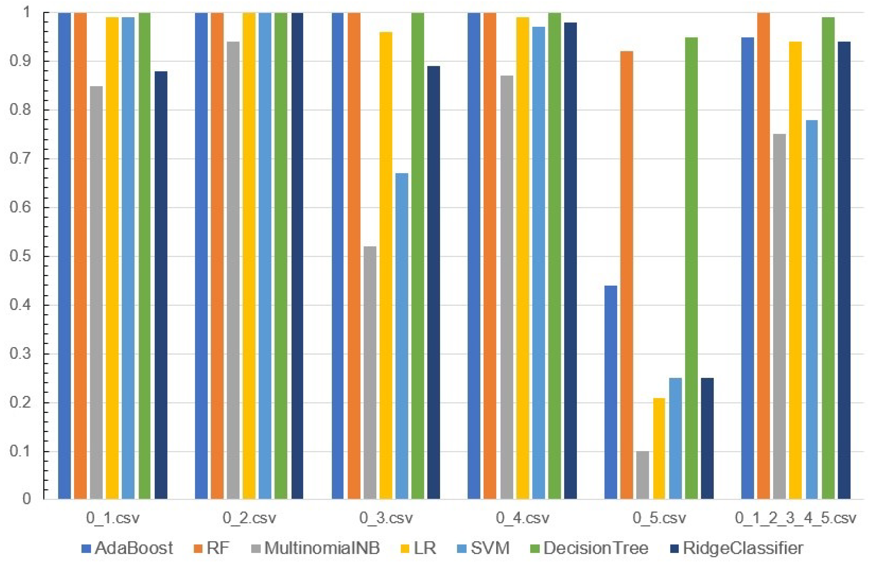
The results of the experiments are shown in Figure 6. It reflects the quality of attack classification by machine learning methods for each input dataset using the f1-score metric.

5.2. Analysis of the Proposed Visualization Efficiency

The goal of the experiments conducted with a visualization component was to determine the most suitable parameters for the calculation of the integral metric $Change\_Measure$, i.e., size of sampling window that defines a number of the points used to construct Delaunay triangulation and enables clear identification of the anomaly. The authors also evaluated the impact of smoothing filters on the visual efficiency to reveal specific classes of attacks.

The experimental data consisted of five data sets that are described in Section 5.1.

To determine the optimal number of data points that are used to construct Delaunay triangulation, the authors calculated and plotted the $Change\_Measure$ metric with the following parameters:

• Distance between 2 points (parameter $n=2$),
• Triangular area by 3 points (parameter $n=3$),
• Delaunay triangulation by 5 points (parameter $n=5$),
• Delaunay triangulation by 10 points (parameter $n=10$).

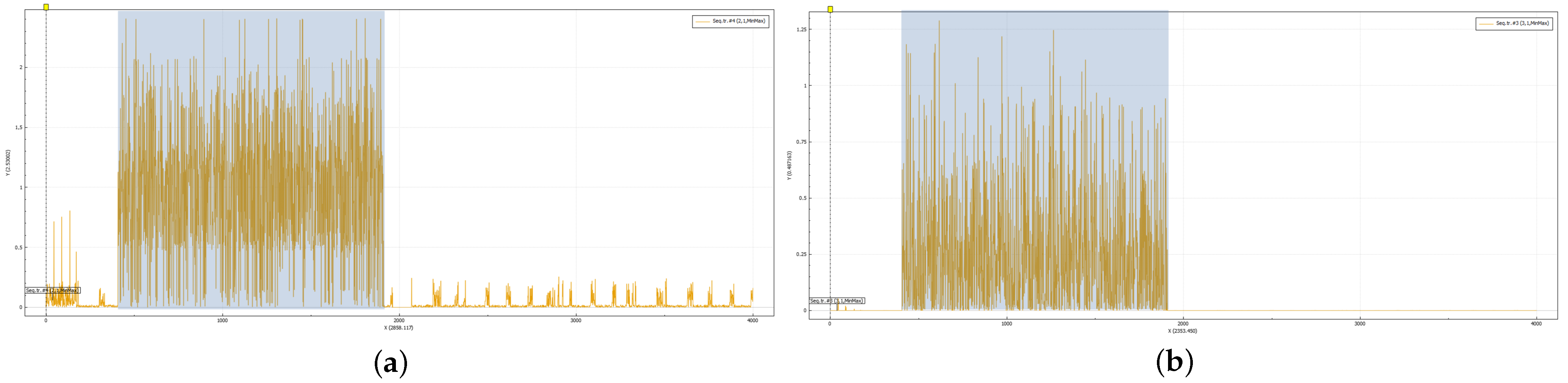
For the test data, the data set with the first class of the attack was used. Figure 7 shows plots of the $Change\_Measure$ metric for these four settings, and the background color shows the time intervals with the attack.

It is obvious that the plots of the metric based on the calculation of triangular squares produce similar patterns of anomalous activity, while the metric based on the calculation of the Euclidean distance between two points gives a slightly different plot (Figure 7a). It is possible to see the transition period at the beginning more clearly, and the normal period of functioning is also characterized by periodical bursts in the metric values. In contrast, the plots of the metrics based on the triangles’ area allow an analyst to detect normal and anomalous periods clearly: the periods of attack are characterized by high scatter in values and higher frequency of change, and the metric values for normal periods are almost close to zero and change slightly. As all plots produce similar results, the metric based on the calculation of the triangle square is preferable because it is faster to calculate and does not require the accumulation of data, which may be critical for the online monitoring of the system. In the next series of experiments, the authors used the $Change\_Measure$ calculated with n set to 3. The next series of experiments was devoted to the evaluation of the efficiency of the $Change\_Measure$ metric to determine different classes of the attack.

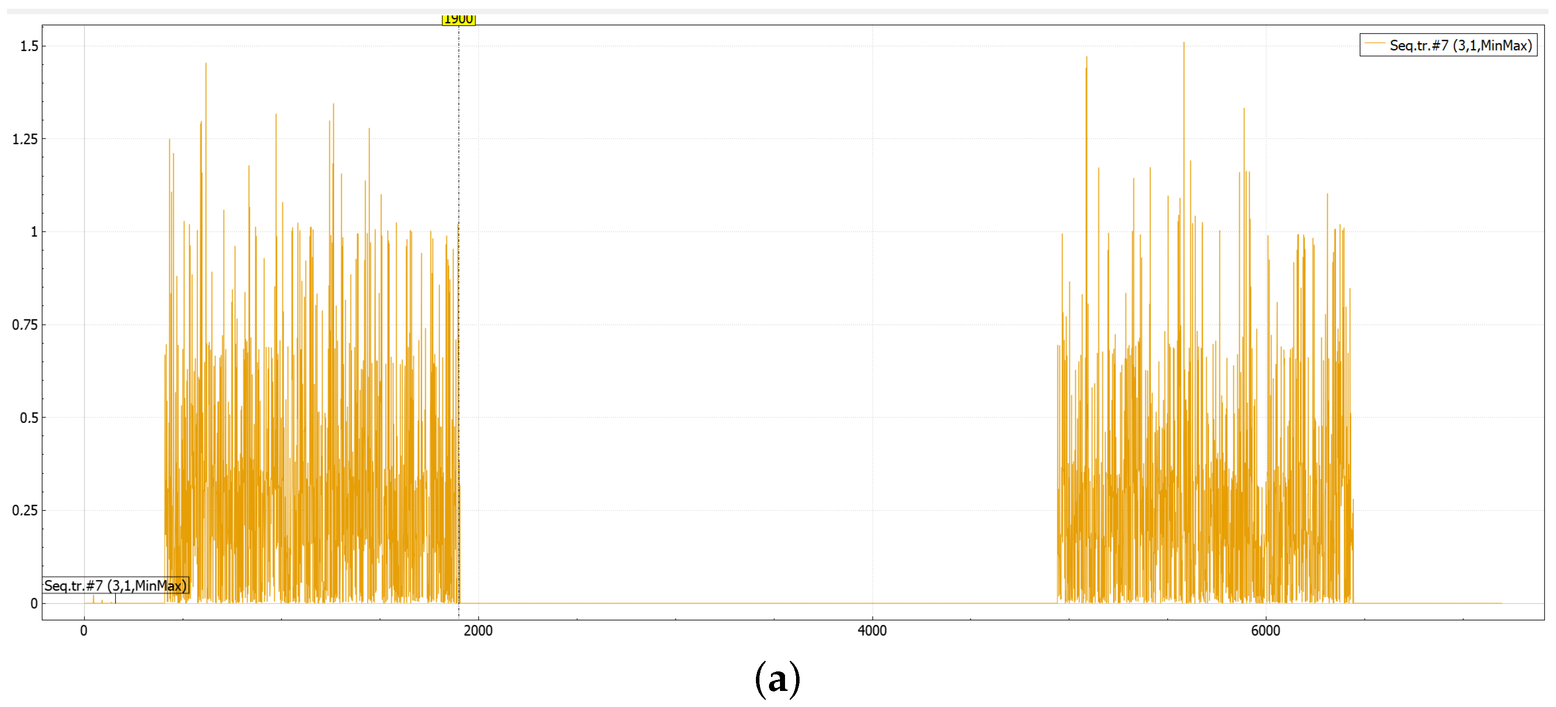
An attack of the first class is clearly seen on the plot of the $Change\_Measure$ metric with different visualization settings. Figure 8 shows these plots, it should be noted that the $Change\_Measure$ metric is constructed for the whole set of attributes. The plot of the “raw” metric is characterized by a constant change of the metric values, the sliding filters smooth these changes making the start and stop points of the attack more visible.

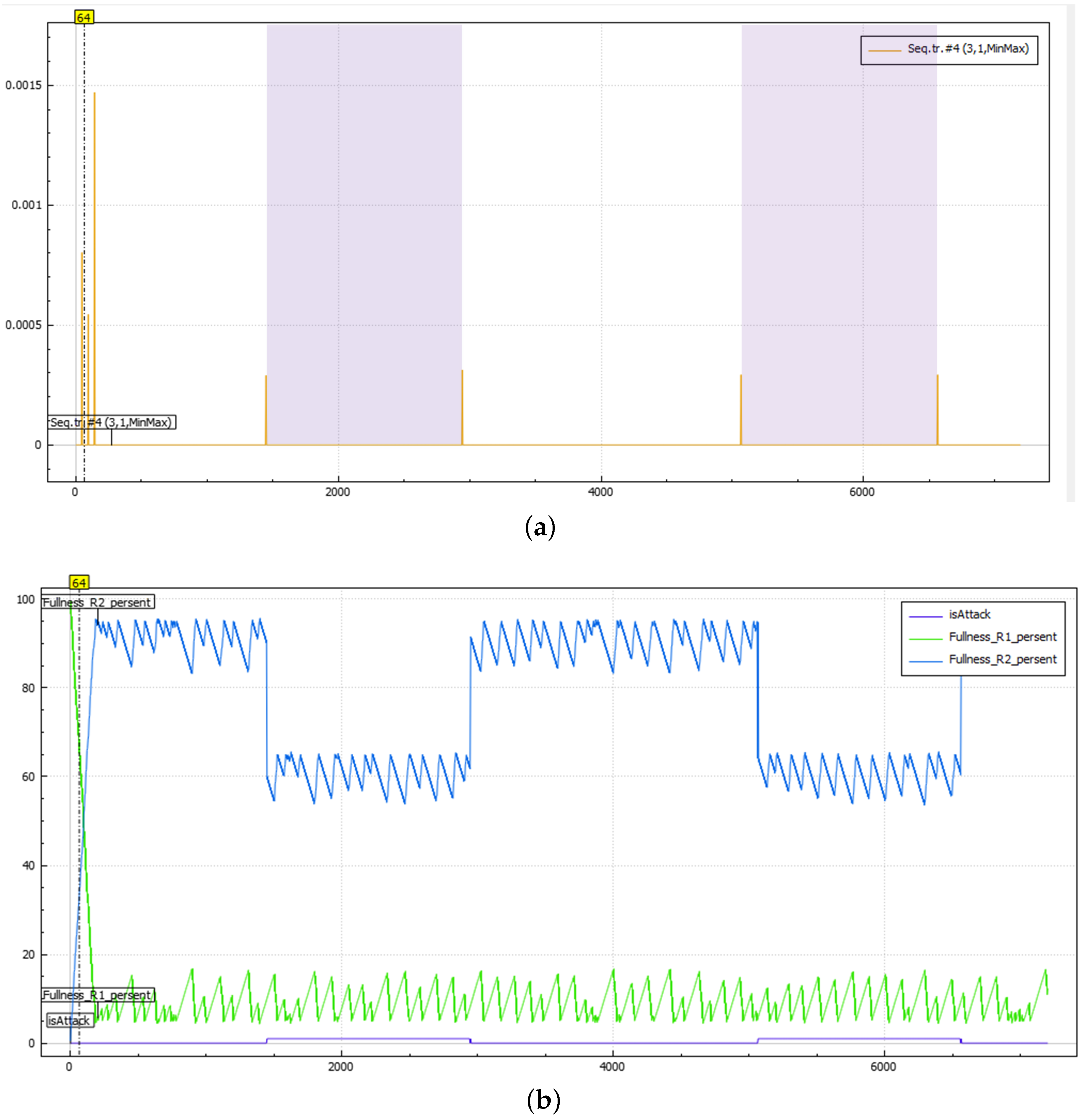
The attack of the second class was not easy to detect as there were no clearly visible changes in the behaviour of the $Change\_Measure$ metric when it was constructed for the whole set of attributes. Thus, it was decided to focus only on the parameters that could be potentially impacted by the attack, i.e., parameters that characterize the volume of the water in the reservoir. This allowed authors to reveal some anomalous spikes in the system’s functioning. Figure 9 shows the plot of the obtained values of the $Change\_Measure$ metric. It is clearly seen that there is a sequence of spikes at the beginning of the plot that could indicate that the system is in a transient state, reaching its normal functioning mode, and there are four single outliers. When the authors mapped the time intervals of the attack with this plot, it became clear that these spikes indicate the start and stop points of the attack. These spikes are clearly visible even when no sliding filters are applied. Thus, it could be concluded that the patterns of system behavior in the normal state and under a given attack do not differ, which indicates that in this case, the proposed method determines only the fact of anomaly appearance, but not its effect on the nature of system operation.

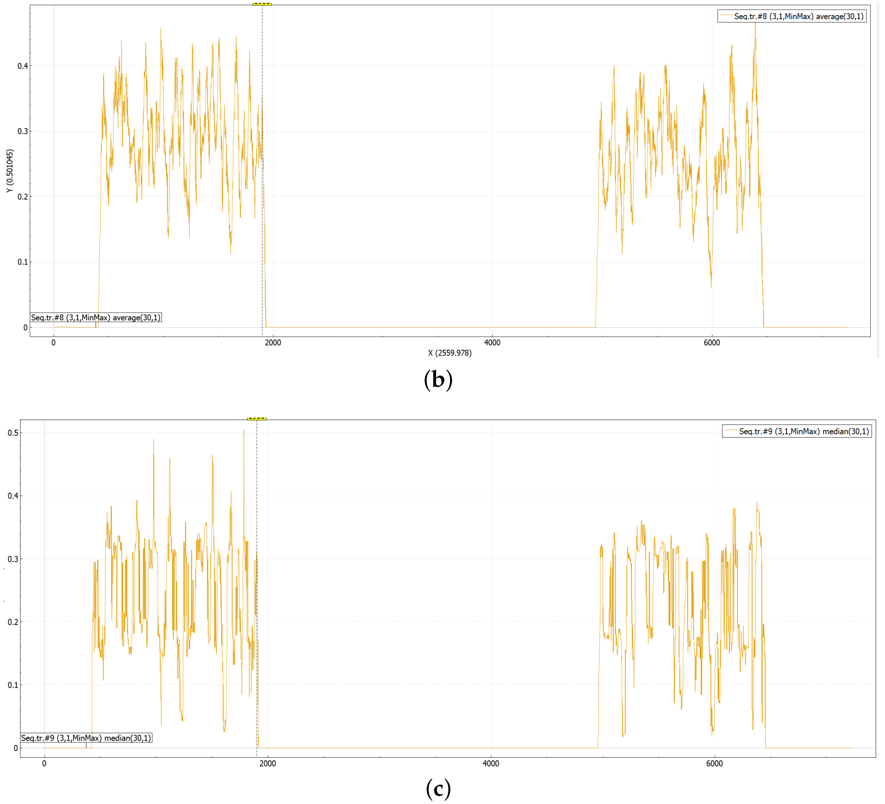
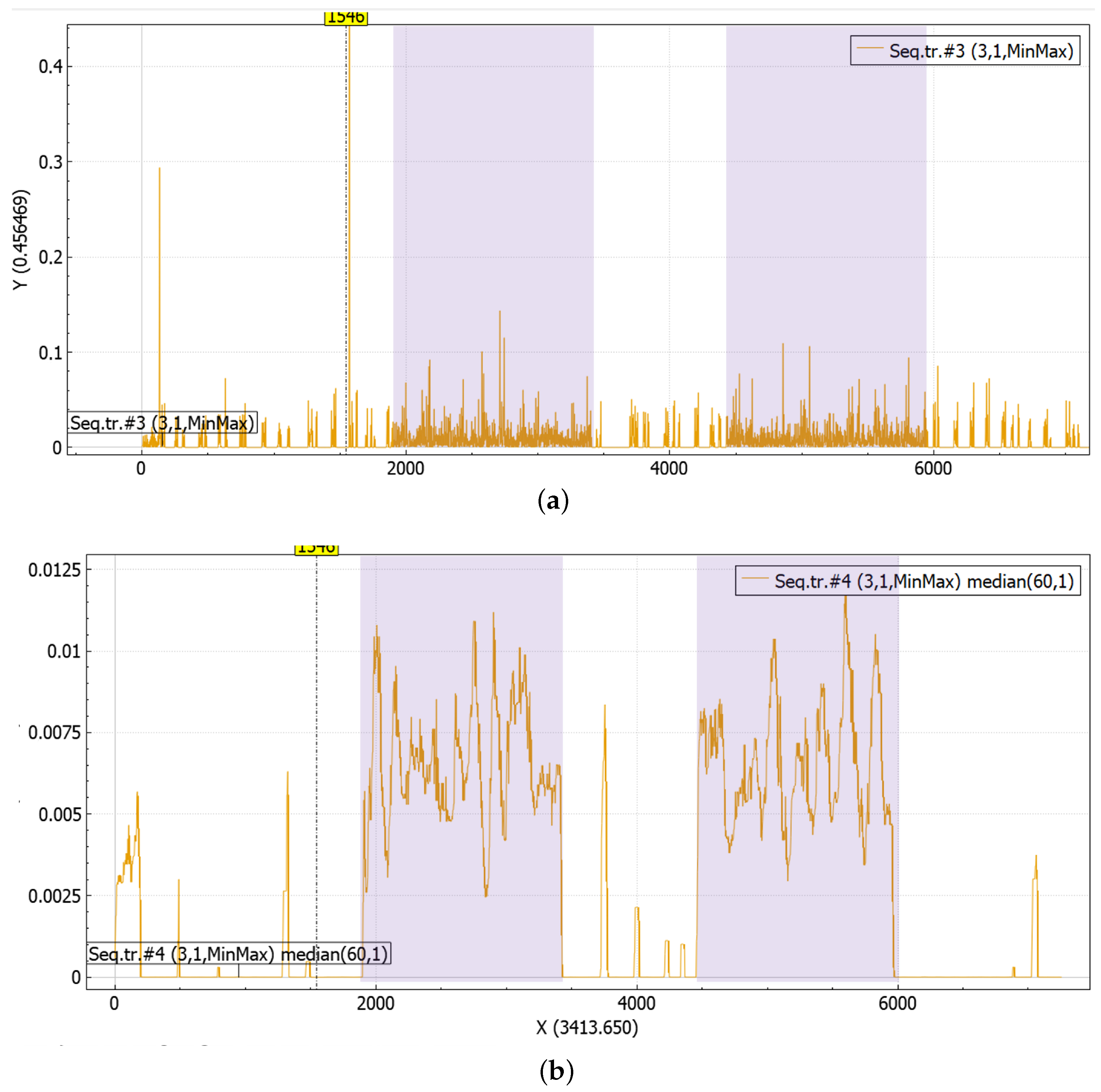
The anomalies of the third and fifth types can be clearly seen on the linear plots without filtering (Figure 10a) and with sliding median filtering with a window set to 60 (Figure 10b). A characteristic feature of these attacks is a significant change in the density of points on the plane that results in the higher values of the $Change\_Measure$ on the plot as well as in the absence of periods with a small change in the system state (Figure 10a). This makes median filtering more effective, enabling highlighting such periods more obviously. As in the previous case with an attack of the second class, there are also bursts at the beginning of the graph, which indicates the transient state of the system when it is reaching the normal operating mode. Such moments should be taken into account when applying this method.

The anomaly of the fifth type turned out to be more difficult to determine visually, although it is a combination of attacks of classes three and four. In contrast to the previous cases, during this attack, the state of the system does not change significantly in comparison with the normal operation of the system, and periods with an anomalous operation, on the contrary, are characterized by lower values of the $Change\_Measure$. Thus, the anomaly pattern for this attack consists in the smaller range of the metrics’ values.

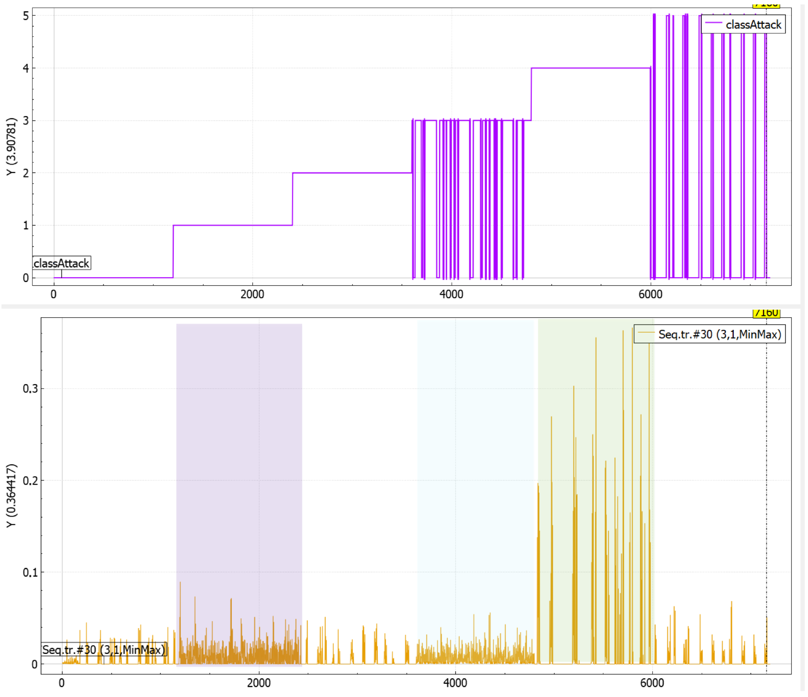
The implemented visualization-driven approach to anomaly detection was also applied to the data set that contains all types of anomalies. Figure 11 shows the results obtained. The upper plot in Figure 11 shows the class of the attack if the system is under attack or zero if there is no anomaly in the system. The lower plot is the plot of the $Change\_Measure$ metric. The anomalies of the first, third and fourth types are clearly seen, and these anomalies are highlighted by a background color in Figure 11. The visual detection of the anomalies of the second and fifth types is much more complicated. Thus, it is required to apply filtering with a sliding average filter with a window of 60 to reveal the attack of the second class, while the attack of the fifth class was still difficult to determine visually. The possible reason for this failure could be in the artificial origin of the data: the periods with anomalies successively replace each other, and there are almost no periods with normal functioning of the system except for the first one, but it corresponds to the transition period of the system when it reaches the normal operational mode.

5.3. Discussion

The analysis of the experimental results with the machine learning models that are given in Figure 6 showed that the performance metrics are very high for some classes of attacks. To avoid overfitting during the experiments, the initial data set was divided into training and testing subsets (with respect to 70/30). This was applied in all series of experiments, including data sets with attacks of the first and second classes. The possible reason for such a high detection rate is the low complexity of these attacks and the high separability of the classes. The latter is proved by good visibility of the periods with attacks when they are visualized using the proposed graphical model. With an increase in the attack complexity as well as their number in the input data set, the performance metrics of machine learning methods slightly decrease but still remain quite high. This proves the efficiency of the proposed solutions.

The implemented series of experiments showed that the proposed visualization technique allows constructing the graphical patterns of the anomalous behavior of the water treatment system. These patterns are formed by the $Change\_Measure$ metric and characterized either by the values of the change metric or by the change rate of these values. It allows identifying points when the functioning of the system changes, which could be used as a trigger to start manual and/or machine-assisted checking of the system state.

Nevertheless, the conducted experiments revealed the limitations of the approach. It was shown that it is required to apply different pre-processing techniques such as median filtering and window size setting in order to reveal different attack scenarios. To solve the first problem, the authors currently recommend implementing the following steps:

• Visualize the “raw” plot of the $Change\_Measure$ metric for the whole set of attributes.
• Apply filter “sliding average filter” to highlight time periods when the rate of the metric change is higher in comparison to others.
• Apply filter “sliding median value” to highlight time periods when the values of the metric are higher in comparison to others
• If no signs of anomaly are detectable, group attributes based on their semantic relationships and perform steps 2–3.

The comparative analysis of the proposed approach with the existing ones showed that with regard to visualization, the proposed approach is close to the solutions described in [19,21]. Similarly to [21], the authors use a timeline to monitor the system’s behavior and machine learning behavior. However, to construct the line chart, the authors introduce a specific preprocessing of data from multiple sensors that, in some sense, is close to [19,20]. Unlike [20], the authors represent the behavior of the whole system by a point in a multidimensional space and then apply the Delaunay triangulation to assess the amount of changes in system behavior at a given moment of time. As the proposed $Change\_Measure$ metric incorporates a set of system parameters, the developed visualization is able to form situational awareness of the water treatment system state.

6. Conclusions

The problem of the attack and anomaly detection in cyber-physical systems, such as water treatment systems, electric power stations, etc., is of great practical importance, as malicious activity may result in a significant impact on the environment and human safety. In the general case, attacks on sensors of a wireless sensor network are characterized by the complexity of identifying such attacks and their differences from various software and hardware/software failures. In addition, they are characterized by the complexity and potential ambiguity of interpreting the analyzed data and classifying them as traces of an attack without involving additional data from alternative protection mechanisms.

The paper proposes a visualization-assisted approach to anomaly and attack detection in a water treatment system constructed on the basis of a wireless sensor network. The distinctive feature of the proposed approach is a combination of the machine learning and visualization techniques. The former refers to automated attack detection based on supervised learning on the labeled data sets with five attack classes and mixed data. The latter is used to assist in anomaly detection and its explanation and the monitoring of the system state. The authors propose visualizing a metric that characterizes the amount of change in the system state for a given period. As its calculation is based on a set of system parameters, it could be considered as an integral and be used in forming the situation awareness of the analyst.

To evaluate the proposed approach, a water treatment test bed was developed. It includes a software/hardware prototype of the system that models water treatment processes both on physical equipment and microcircuits, as well as a software simulator that allows generating a sufficient amount of initial data of the normal functioning of the system and when the system is under attack. In particular, such simulation made it possible to model five classes of attacks on system sensors and combinations of several attacks. The obtained data sets were used to train and test classifiers that implement attack detection and evaluate the efficiency of the visualization component.

The conducted experiments showed the high values of the detection quality metrics for the machine learning methods applied. It was also shown that the proposed visualization is able to reveal different anomalous scenarios and determine graphical patterns corresponding to them. It allows detecting points of interest that are considered as a starting point of the manual or machine-assisted “root-cause” analysis of the anomalies. However, the experiments also identified certain limitations in terms of the visualization. They relate to the parameters’ fine-tuning procedure for calculation and visualization of the proposed metric. The enhancement of the metric calculation procedure and elaboration of the recommendations for its application is included in the scope of future works. Another direction of the future work relates to the enhancement of the test bed and extension of the modeled attack scenarios.

References

- Shin, J.; Baek, Y.; Eun, Y.; Son, S.H. Intelligent sensor attack detection and identification for automotive cyber-physical systems. In Proceedings of the 2017 IEEE Symposium Series on Computational Intelligence (SSCI), Honolulu, HI, USA, 27 November–1 December 2017; pp. 1–8. [Google Scholar] [CrossRef]
- Rehman, A.u.; Rehman, S.U.; Raheem, H. Sinkhole Attacks in Wireless Sensor Networks: A Survey. Wirel. Pers. Commun. 2019, 106, 2291–2313. [Google Scholar] [CrossRef]
- Wang, R.; Song, H.; Jing, Y.; Yang, K.; Guan, Y.; Sun, J. A Sensor Attack Detection Method in Intelligent Vehicle with Multiple Sensors. In Proceedings of the 2019 IEEE International Conference on Industrial Internet (ICII), Orlando, FL, USA, 11–12 November 2019; pp. 219–226. [Google Scholar] [CrossRef]
- Inoue, J.; Yamagata, Y.; Chen, Y.; Poskitt, C.M.; Sun, J. Anomaly Detection for a Water Treatment System Using Unsupervised Machine Learning. In Proceedings of the 2017 IEEE International Conference on Data Mining Workshops (ICDMW), New Orleans, LA, USA, 18–21 November 2017; pp. 1058–1065. [Google Scholar] [CrossRef] [Green Version]
- Park, J.; Ivanov, R.; Weimer, J.; Pajic, M.; Lee, I. Sensor attack detection in the presence of transient faults. In Proceedings of the ACM/IEEE Sixth International Conference on Cyber-Physical Systems, ICCPS 2015, Seattle, WA, USA, 14–16 April 2015; Bayen, A.M., Branicky, M.S., Eds.; ACM: New York, NY, USA, 2015; pp. 1–10. [Google Scholar] [CrossRef] [Green Version]
- Rahim, M.S.; Nguyen, K.; Stewart, R.; Giurco, D.; Blumenstein, M. Machine Learning and Data Analytic Techniques in Digital Water Metering: A Review. Water 2020, 12, 294. [Google Scholar] [CrossRef] [Green Version]
- Raciti, M.; Cucurull, J.; Nadjm-Tehrani, S. Anomaly Detection in Water Management Systems. In Lecture Notes in Computer Science. Critical Infrastructure Protection: Information Infrastructure Models, Analysis, and Defense; Springer: Berlin/Heidelberg, Germany, 2012; pp. 98–119. [Google Scholar] [CrossRef]
- Banerjee, K.; Bali, V.; Nawaz, N.; Bali, S.; Mathur, S.; Mishra, R.K.; Rani, S. A Machine-Learning Approach for Prediction of Water Contamination Using Latitude, Longitude, and Elevation. Water 2022, 14, 728. [Google Scholar] [CrossRef]
- Naloufi, M.; Lucas, F.; Souihi, S.; Servais, P.; Janne, A.; Abreu, T. Evaluating the Performance of Machine Learning Approaches to Predict the Microbial Quality of Surface Waters and to Optimize the Sampling Effort. Water 2021, 13, 2457. [Google Scholar] [CrossRef]
- Shulepov, A.; Novikova, E.; Murenin, I. Approach to Anomaly Detection in Cyber-Physical Object Behavior. In Intelligent Distributed Computing (IDC-2021); Springer International Publishing: Cham, Switzerland, 2021; pp. 417–426. [Google Scholar] [CrossRef]
- Herr, D.; Beck, F.; Ertl, T. Visual Analytics for Decomposing Temporal Event Series of Production Lines. In Proceedings of the 2018 22nd International Conference Information Visualisation (IV), Fisciano, Italy, 10–13 July 2018; pp. 251–259. [Google Scholar]
- Shi, Y.; Liu, Y.; Tong, H.; He, J.; Yan, G.; Cao, N. Visual Analytics of Anomalous User Behaviors: A Survey. IEEE Trans. Big Data 2022, 8, 377–396. [Google Scholar] [CrossRef] [Green Version]
- Ji, S.Y.; Jeong, B.K.; Jeong, D.H. Evaluating Visualization Approaches to Detect Abnormal Activities in Network Traffic Data. Int. J. Inf. Secur. 2021, 20, 331–345. [Google Scholar] [CrossRef]
- Jin, Z.; Guo, S.; Chen, N.; Weiskopf, D.; Gotz, D.; Cao, N. Visual Causality Analysis of Event Sequence Data. IEEE Trans. Vis. Comput. Graph. 2021, 27, 1343–1352. [Google Scholar] [CrossRef] [PubMed]
- Visplore—Software for Visual Time Series Analysis. 2022. Available online: https://visplore.com/ (accessed on 21 March 2022).
- Toshiba IoT Solution Pack. 2017. Available online: http://www.toshiba.com/solutions/iot-solution-pack.html (accessed on 21 December 2021).
- Kaspersky Machine Learning for Anomaly Detection. 2017. Available online: https://mlad.kaspersky.com/ (accessed on 21 March 2022).
- Janetzko, H.; Stoffel, F.; Mittelstädt, S.; Keim, D.A. Anomaly detection for visual analytics of power consumption data. Comput. Graph. 2014, 38, 27–37. [Google Scholar] [CrossRef] [Green Version]
- Novikova, E.; Bestuzhev, M.; Kotenko, I. Anomaly Detection in the HVAC System Operation by a RadViz Based Visualization-Driven Approach. In Computer Security; Katsikas, S., Cuppens, F., Cuppens, N., Lambrinoudakis, C., Kalloniatis, C., Mylopoulos, J., Antón, A., Gritzalis, S., Pallas, F., Pohle, J., et al., Eds.; Springer International Publishing: Cham, Switzerland, 2020; pp. 402–418. [Google Scholar]
- Steiger, M.; Bernard, J.; Mittelstädt, S.; Lücke-Tieke, H.; Keim, D.A.; May, T.; Kohlhammer, J. Visual Analysis of Time-Series Similarities for Anomaly Detection in Sensor Networks. Comput. Graph. Forum 2014, 33, 401–410. [Google Scholar] [CrossRef]
- Wu, W.; Zheng, Y.; Chen, K.; Wang, X.; Cao, N. A Visual Analytics Approach for Equipment Condition Monitoring in Smart Factories of Process Industry. In Proceedings of the 2018 IEEE Pacific Visualization Symposium (PacificVis), Kobe, Japan, 10–13 April 2018; pp. 140–149. [Google Scholar] [CrossRef]
- Streaming Visual Analytics Workshop Report. 2016. Available online: https://www.pnnl.gov/main/publications/external/technical_reports/PNNL-25266.pdf (accessed on 21 December 2021).
- Shulepov, A.; Novikova, E.; Bestuzhev, M. Approach to Compare Point Distribution Patterns Produced by Dimension Reduction Techniques. In Proceedings of the 2021 IEEE Conference of Russian Young Researchers in Electrical and Electronic Engineering (ElConRus), St. Petersburg, Russia, 26–29 January 2021; pp. 678–681. [Google Scholar] [CrossRef]
- Meleshko, A.; Desnitsky, V.; Kotenko, I.; Novikova, E.; Shulepov, A. Combined Approach to Anomaly Detection in Wireless Sensor Networks on Example of Water Management System. In Proceedings of the 2021 10th Mediterranean Conference on Embedded Computing (MECO), Budva, Montenegro, 7–10 June 2021; pp. 1–4. [Google Scholar] [CrossRef]
Figure 1.
The scheme of the proposed visualization assisted anomaly and attack detection approach.
Figure 2.
The GUI of the visualization component: (A)—a view for displaying system parameters that are selected by an operator; (B)—a plot of the integral metric , the background color shows the periods when the system was under the attack.
Figure 3.
The scheme of the case study.
Figure 4.
Scheme of the simulation algorithm.
Figure 5.
Architecture of the used experimental framework for the classification.
Figure 6.
Machine learning method results comparison (f1-score).
Figure 7.
Plot of the metric constructed for different settings of the n parameter: (a), (b), (c), and (d).
Figure 8.
Plot of the metric constructed for different settings of the sliding filter: no filter is applied (a), sliding average filter with the window set to 30 is applied (b), sliding median filter with the window set to 30 is applied (c).
Figure 9.
System parameters and metric when the system is under attack of the second class: the plot of metric with background color highlighting the periods with attacks (a), the plots of system parameters that characterize the volume of the water in the reservoirs (b).
Figure 10.
Plot of the metric constructed for the system under attack of the third class: no filter is applied (a), sliding median filter with the window set to 60 is applied (b).
Figure 11.
The visualization of the metric constructed for the data set that contains all five different types of anomalies. The upper plot shows if the system is under attack or not, and if the system is under attack it shows the class of the attack.