Climate Change Impacts on Hydrological Processes in a South-Eastern European Catchment

Abstract

The output extracted from CNRM, MPR, and ICHEC Global Circulation Models for RCP 4.5 and RCP 8.5 Representative Concentration Pathways has been used in conjunction with the SWAT model for evaluating the impacts of future climate changes on hydrological processes in a Romanian catchment (Neajlov, 3720 km² area) in the short (2021–2050) and long term (2071–2100). During the growing season, precipitation will decrease by up to 7.5% and temperature will increase by up to 4.2 °C by 2100. For the long term (2071–2100), the decrease in soil water content (i.e., 14% under RCP 4.5 and 21.5% under RCP 8.5) and streamflow (i.e., 4.2% under RCP 4.5 and 9.7% under RCP 8.5) during the growing season will accentuate the water stress in an already water-deficient area. The snow amount will be reduced under RCP 8.5 by more than 40% for the long term, consequently impacting the streamflow temporal dynamics. In addition, our results suggest that hydrological processes in the lower portions of the catchment are more sensitive to climate change. This study is the first Romanian catchment-scale study of this nature, and its findings support the development of tailored climate adaptation strategies at local and regional scales in Romania or elsewhere.

1. Introduction

Climate projections based on current greenhouse gases emissions predict that global mean surface temperatures for 2081–2100, relative to 1986–2005, will likely be from 0.3 °C to 1.7 °C (RCP 2.6), 1.1 °C to 2.6 °C (RCP 4.5), 1.4 °C to 3.1 °C (RCP 6.0), and 2.6 °C to 4.8 °C (RCP 8.5) [1]. If these changes take place, the atmosphere will be warmer than it has been at any time during the past 125,000 years [1]. The warming will be accompanied by changes in many other environmental variables, including precipitation amount and regime, and hence, due to the integrated nature of the hydrological cycle will change most of its components [1,2,3]. At the European scale, it is anticipated that the future climate changes will vary at local and regional scales, with a series of studies underlining the uncertainties associated with the patterns and amplitude of the changes [1,4,5,6,7]. Examples of impacts include increased pluvial flooding in northern Europe and hydrological and agricultural/ecological droughts in the Mediterranean region, as well as significant changes to key components of the hydrological cycle, such as snow accumulation and surface runoff by the end of the century [7]. For Eastern Europe, the RCP 8.5 projection indicates that temperature will increase with 1.5 to 4 °C during both the winter and summer by 2041–2060 [1]. Precipitation will also be impacted and might increase by up to 20% during the winter and decrease by up to 20% during the summer for the same period [1].

The assessment of the impacts of climate changes on hydrological processes via modeling is recognized as an important tool that provides support for policy makers and water resource managers to develop adaptation measures and elaborate management strategies related to socio-ecological systems [1,8,9,10]. At the European level, hydrological modeling has been employed for predicting hydrological conditions in a changing climate [11,12,13]. However, these large-scale models might lack the spatial resolution that can be achieved with local-scale models, generally are subject to a global calibration procedure, and might not operate using hydrological entities (i.e., watersheds) as basic units [14,15]. Currently, watershed or even regional-scale studies in Eastern Europe are limited. For example, [16] used non-climate model-based scenarios in a study covering the Black Sea catchment and found that a 3 °C increase in temperature combined with a 30% decrease in precipitation amount will result in decreased soil moisture which in turn will result in increased irrigation demand and potentially increased competition for water resources. In a pan-European study conducted using WaterGAP3 model [17], Beek et al. (2012) [11] found that the mean annual water availability for Romania will be reduced by 5–15% by 2050 under the A2 IPCM4 and MIMR IPCC scenarios [18]. Freund et al. (2017) [19] employed the SWAT model to evaluate potential impacts of future climate changes (2017–2050) on water resources in the Black Sea catchment using A2 and B2 IPCC scenarios [18] combined with four land use change scenarios developed using enviroGRIDS [20] and found that areas of the Black Sea catchment, including Romania, will experience a decrease in water storage, which could lead to increased vulnerability of freshwater resources. The authors also estimated that “blue water” (i.e., the sum of streamflow and aquifer recharge) in the southern part of Romania will decrease between 0 and 50% based on the average output of 10 scenarios. Didovets et al. (2017) [21] employed the Soil and Water Integrated Model (SWIM; [22]) to assess the impact of RCP 4.5 and RCP 8.5 [1] on water resources for the near future (2011–2040), middle future (2041–2070), and far future (2071–2100) in three Ukrainian catchments. Out of the three catchments, the Samara catchment, which is most similar to the catchment used in our study, is expected to experience a slight increase in streamflow for the near and middle future (+10–20%) and a decrease in the far future (~10%). The authors also suggest that the streamflow is expected to increase during the winter and spring season and decrease during the summer. For Romania, only two relevant studies have been identified. The first study was conducted in the early 2000s by Cuculeanu et al. (2002) [23] at a Romanian national scale. The study involved a combination of plant growth, forest dynamics, and rainfall–runoff models and found that by 2070, snowmelt will occur earlier in the year, the maximum stream discharge will shift from spring towards the winter months, and the minimum flows will shift from October–January to August–October in response to an increase in temperature between 2.8 and 4.9 °C, a ~20% increase in precipitation during the cold season, and a decrease by a similar amount during the warm season compared to the reference state (1961–1990). A second study, carried out by Mitrica et al. (2017) [24] in the southern part of Romania (Leu-Rotunda Plain; 650 km²), in an area with similar climate with the Neajlov catchment, employed a combination of groundwater numerical modeling and regional climate model simulations to understand the impact of future climate changes (2017–2100) on aquifer water availability. Their results suggest that aquifer water resources will decrease by ~10% between 2021 and 2050 and by ~30% between 2071 and 2100 for the respective area compared to the reference period (1961–1990), thus pointing to significant vulnerability in the water supply in the future, in an area that is already water-deficient and scarce in water resources.

The present study aims at assessing the impacts of short- (i.e., 2021–2050) and long-term (2071–2100) future climate changes associated with two RCPs (i.e., RCP 4.5 and RCP 8.5) on the magnitude and variability of hydrological processes in a medium-sized catchment located in the southern part of Romania (Neajlov catchment, 3720 km²). The hydro-climatic model developed in SWAT [25] has been calibrated for the reference state using 30 years of daily weather and streamflow data (1981–2010) collected from various stations within the catchment and has been run with a monthly output frequency between 2010 and 2100 using the full array of climate data produced with three GCMs (CNRM, MPR, ICHEC) [26]. This is the first study that uses long-term historical and future climate data for evaluating the impacts of future climate changes on hydrological processes at a Romanian catchment scale and contributes to advancing the understanding of the extent of future climate change impacts on hydrological processes both in Romania and in Eastern Europe at large, a region where previous studies are limited. In addition, the results of this study provide an additional resource for inter-comparison of results obtained through similar studies carried out in other regions of Europe or the world. The findings of this study can be used for assisting policy makers and water resource managers in adapting mid- and long-term strategies to better respond to anticipated climate changes, as highlighted in recent European [27] and global-scale forums [28].

2. Materials and Methods

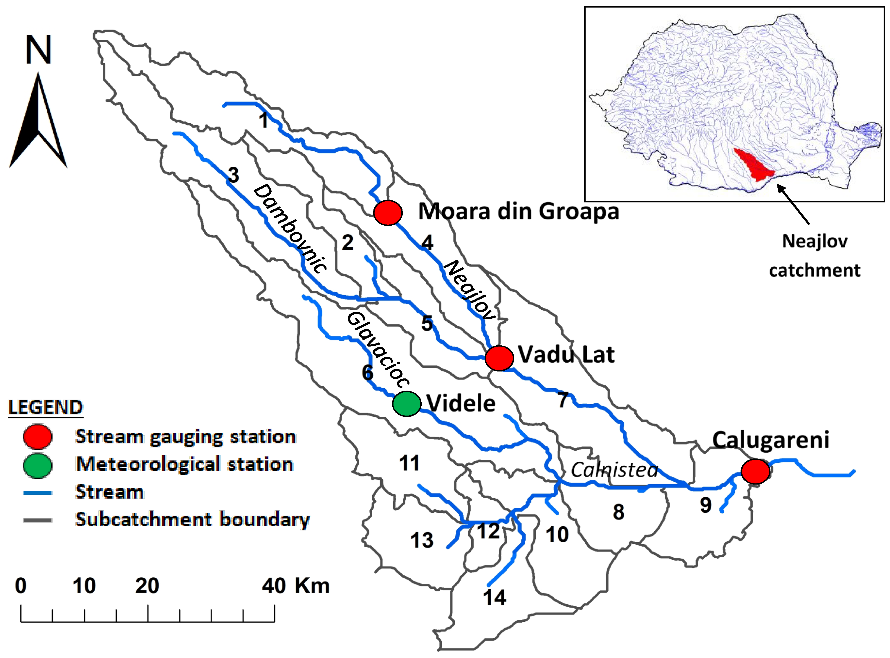
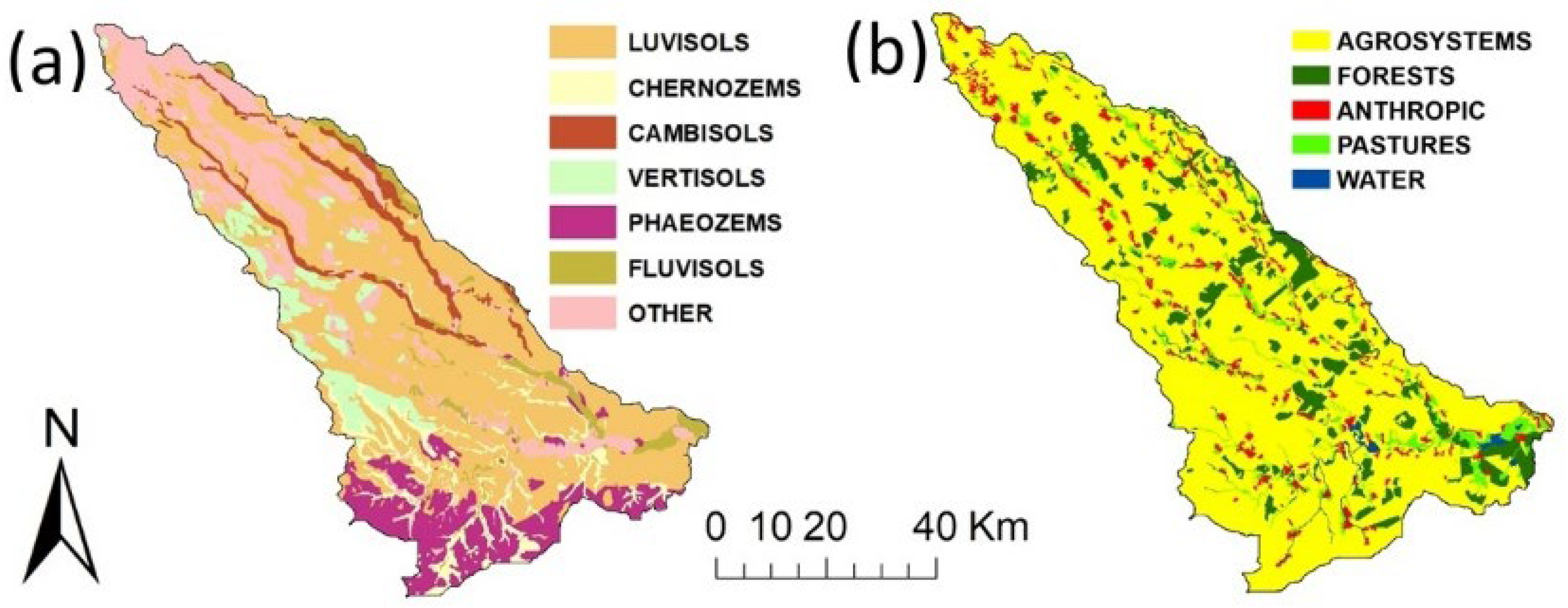
2.1. Study Area

Located in the southern part of Romania (i.e., Romanian Plain), between 43°56′00″ N-44°49′12″ N latitude and 24°14′30″ E-26°15′36″ E longitude, the Neajlov catchment is the largest subcatchment (3720 km²) of the Arges River, a tributary of the Danube River (Figure 1). Due to its importance as a Danube subbasin, the Neajlov catchment is critical for a deep understanding of the processes that occurs in the Romanian plain and has been incorporated in the LTSER (Long-Term Socio-Ecological Research) network [29] since 2007. The catchment is characterized by large parallel valleys oriented from NW to SE and gentle slopes, ranging between 1–2‰ in the lower Neajlov catchment and 3–4‰ in the upper Neajlov catchment. The elevation is gradually decreasing from north (~300 m) to south (~60 m). The main tributaries of Neajlov are Dambovnic, Glavacioc, and Calnistea (Figure 1), and its hydrographic network has an average density of 0.36 km/km², which is similar to the average for Romanian water courses [30]. The average stream discharge measured at the outlet of the catchment (i.e., Calugareni) is ~7.7 m³/s (1981–2010) [31]. The maximum flows are dominantly occurring during early spring but can occur during any period of the year as a result of either snowmelt or significant rainstorms and can be up to 160 times higher than the annual average discharge [30]. This period of high flows is followed by an extended period of recession and low flows through the summer and fall, when the stream flow is provided exclusively from the aquifer [32,33] and the discharge of Neajlov can be lower than 1 m³/s, while its main tributaries can have flows as low as 0.03 m³/s [30].

The subsurface material consists of sedimentary deposits of variable thicknesses. The quaternary deposits are of fluvio-lacustrine origin and consist of sand and gravel deposits (i.e., Fratesti-Candesti deposits) underlining 10–20 m thick loess or loessial deposits [30,32]. Based on the FAO soil classification [34], the soils in the catchment are dominated by luvisols (61% of the catchment area), which are generally fertile soils widespread in the temperate regions, while other soils such as chernozems, cambisols, vertisols, phaeozems, and fluvisols cover less than 10% of catchment area each (Figure 2a). Land cover in the catchment is dominated by agrosystems (77.8% of the catchment area), followed by forests (10.4%), anthropic systems (i.e., industrial, residential; 5.6%), pastures (5.1%), and water (i.e., surface water bodies and wetlands; 1.1%) (Figure 2b). Rural settlements are prevalent in the catchment and major urban areas are absent.

The climate of Romania is temperate-continental, with influences from Atlantic and Mediterranean air masses in the western regions, while the southern and eastern regions, where the study area is located, are affected by continental air masses. The climate data collected from Videle meteorological station between 1981 and 2010 [35] (Figure 1) indicate that the mean annual temperature for the entire period is 11.2 °C and varied between 9.7 °C (1985) and 12.8 °C (2007). The annual precipitation amount ranged between 306.8 mm (2000) and 871 mm (2005), an average of 525.7 mm/year for the same period. During the year, the months of June and July received the largest amounts of precipitation (i.e., 64.6 and 65.7 mm, respectively), while January and February recorded the lowest amounts (i.e., 32.3 and 29.0 mm, respectively). Snowfall for the same period represented about 18.2% from the total precipitation, with the snowfall period extending between November and March.

2.2. Modeling

We used the ArcGIS extension of the Soil and Water Assessment Tool (SWAT) (ArcSWAT; [36]) to analyze the effects of predicted climate changes on hydrological processes in the Neajlov River Catchment. SWAT [25] is a widely used distributed parameter, a continuous time model, developed to simulate and predict the impacts of land cover, land use, and climate change on the quantity and quality of both surface and groundwater. SWAT allows various physical processes, such as processes associated with the water and sediment movement, crop growth, and nutrient cycling, to be simulated in a catchment. For modeling purposes, in SWAT, a catchment may be partitioned into subcatchments. Based on the best fit between SWAT delineated streams and hydrographic network maps (e.g., number of tributaries, length of the watercourses, shape of the boundary for the catchment), a threshold of 130 km² catchment area for defining a permanent stream and for delineating the Neajlov catchment and its subcatchments has been used. The Hydrologic Response Units (HRUs), representing key components in SWAT architecture, are areas within the subcatchment that are composed of unique land cover, soil, and management combinations. The Hydrological Response Units (HRUs) required for running the SWAT model were defined using the “multiple HRUs in a subcatchment” ArcSWAT option, with minimum thresholds for land use type (15%) and soil class percentages (15%) for each subcatchment for identifying an HRU.

2.3. Data (Reference State)

The data required for SWAT parameterization included catchment-scale data sets (i.e., Digital Elevation Model (DEM), soil type and land cover) and meteorological data time series. The catchment-scale data processing is presented in detail in [37]. The DEM was developed from 1:100,000 topographic maps covering an area extending beyond the boundaries of the Neajlov catchment. The Neajlov catchment, its subcatchments, and its hydrographic network have been delineated using the watershed delineation routine incorporated in ArcSWAT. The soil spatial distribution was derived from 1:200,000 national soil maps. Soil properties were incorporated into the ArcSWAT user soil database using the equivalency between the map-based soils, which were defined using the Romanian soil classification system, and the properties of the soils available in the ArcSWAT user soil database (e.g., hydrologic group, soil horizons, texture, organic matter content, etc.). The data required for ArcSWAT’s land use layer were extracted from the CORINE Land Cover Database [38], followed by the conversion of specific land cover classes into SWAT equivalent land use categories. Daily meteorological data (i.e., air temperature, precipitation, relative air humidity, wind speed, and solar radiation) between 1981 and 2010 (i.e., 30 years) were obtained from the Videle (44°17′40″ N latitude and 25°32′31” E longitude) meteorological station [35], located centrally in the catchment (Figure 1). The hydrological model was calibrated using the SPE (SWAT Parameter Estimator) program included in SWAT Cup Premium v 6.1.1.0 [39] with daily discharge data measured between 1981 and 2010 at Moara din Groapa (upper catchment), Vadu Lat (mid-catchment), and Calugareni (catchment outlet) (Figure 1) [31]. To improve the stability of the model solution a 30-year model “warm-up” period (1951–1980), consisting of a copy of the 1981–2010 measured meteorological dataset, was added at the beginning of the simulation, as recommended in the literature [25]. The model runs were conducted with a monthly output frequency. The parameters that were adjusted during calibration were selected based on the literature [19,40,41,42]. The calibration parameters were grouped by model subcomponents (i.e., snow processes, groundwater, soil, and stream channel; Table S1) and the calibration was conducted in several cycles of at least 800 simulations each, with each cycle containing a sequence of these groups, as suggested in the literature [39,42]. The efficiency of the model was evaluated using the Nash–Sutcliffe coefficient [43] calculated for measured vs. modeled flows at the three stream gauging stations mentioned above. The Nash–Sutcliffe coefficient ranges from −∞ to 1, with a value of 1 indicating a perfect match between measured and modeled values, values between 0 and 1 indicating acceptable levels of model performance, and negative values indicating unacceptable performance. The calibration was considered complete when additional iterations did not result in further improvement of the Nash–Sutcliffe coefficient.

2.4. Climate Change Scenarios

The impacts of each climate change model on hydrological processes have been evaluated for the reference period (1981–2010), short term (2021–2050), and long term (2071–2100) using two Representative Concentration Pathways (RCPs) [1]. The selected RCPs were RCP 4.5 (moderate; radiative forcing to stabilize at 4.5 W/m² before the year 2100) and RCP 8.5 (business-as-usual; radiative forcing to stabilize at 8.5 W/m₂ before the year 2100). For each RCP, three bias-corrected EURO-CORDEX RCMs nested by Global Circulation Models (GCMs) ([26];

Table 1. Regional Climate Models selected in the study.

No.	Institution or Working Group	RCM Model	GCM Institute	GCM Driving
1	Climate Limited-area Modeling Community (CLMcom)	CCLM4-8-17	CNRM-CERFACS	CNRM-CM5
2	Danish Meteorological Institute (DMI)	HIRHAM5	ICHEC	EC-EARTH
3	Climate Limited-area Modeling Community (CLMcom)	CCLM4-8-17	MPI-M	MPI-ESM-LR

), available at 0.11° spatial resolution (about 12.5 km × 12.5 km), were used to extract the daily meteorological data for the historical (1981–2010) and future simulation periods (2011–2100). Although there could be challenges related to the performance of RCMs in complex terrain [44], the application of the combination of the above RCMs was considered reasonable based on the tests conducted in an area with similar climate to the study area [45]. A separate ArcSWAT simulation was set up for each climate model and RCP. For each of these simulations, the parameters obtained from the SWAT calibrated model were used in conjunction with the daily meteorological data extracted from the climate models for understanding the effects of future climate changes on Neajlov catchment hydrology. The outputs from each climate model and RCP ArcSWAT simulation were averaged and used for assessing the impact of the ensemble of the climate change models (i.e., ENS RCP 4.5 and ENS RCP 8.5) on the water balance.

The analysis was carried both spatially (i.e., subcatchments) and temporally using key water balance components (e.g., stream discharge, soil water content, surface and subsurface runoff, snowfall and snowmelt, evapotranspiration). The output from both the climate models and SWAT model were subsequently integrated over month, growing season (i.e., April to September), annual, decadal, and for each period analyzed. In addition, a representative year was developed by averaging the values of the parameters of interest for any given month in all the years considered for each of the analyzed periods (e.g., the monthly value of the representative year for January was obtained by averaging the parameter values for each January during the period of interest).

3. Results and Discussion

3.1. Model Calibration

The delineation of subcatchments in SWAT resulted in 14 subcatchments, with Moara din Groapa located at the outlet of subcatchment 1, Vadu Lat at the confluence of subcatchments 4 and 5 (i.e., collecting flow from subcatchments 2 to 5), and Calugareni at the outlet of the Neajlov catchment (Figure 1), while the delineation of the Hydrological Response Units (HRUs) required by SWAT was based on using the multiple HRUs in a subcatchment ArcSWAT option, with a threshold of 15% land use type and 15% soil class percentages in each subcatchment, and resulted in 30 HRUs for the Neajlov catchment. The parameters used for the calibration of the model were divided into three groups as follows: (i) groundwater, (ii) snow, and (iii) soil and stream channel (Table S1). The most significant challenge for the calibration of the model was related to the simulation of the snowfall and snowmelt, which is consistent with the findings of other studies relative to the ability of the SWAT model to reproduce these processes [46,47,48]. In this case, neither the automated SPE algorithm included in SWAT-CUP Premium nor the manual trial and error calibration procedures resulted in significant improvement of the timing and magnitude of the modeled streamflow values for the years with extreme peak flows during mid-winter to mid-spring period. These limitations were deemed acceptable, considering that the SWAT simulations were aimed at understanding the long-term dynamics (i.e., multiyear averages) of water balance components.

The average modeled stream discharge for the calibration period (i.e., 1981–2010) was within 10% of the measured stream discharge for each of the three stations (i.e., 1.01 vs. 0.96 m³/s for Moara din Groapa, 4.43 vs. 4.24 m³/s for Vadu Lat, and 7.72 vs. 8.47 m³/s for Calugareni) (Figures S1–S3). The final Nash–Sutcliffe coefficient (NS) values for the monthly model output were 0.36, 0.28, and 0.39 for Moara din Groapa, Vadu Lat, and Calugareni, respectively. On an annual basis, the NS for the three calibration locations increased to 0.64, 0.33, and 0.52. Although the match between modeled and measured values of stream discharge was only moderate, this was considered reasonable given the high intra- and interannual variability in streamflow as well as the unavailability of data related to water use and management in the Neajlov catchment. Abbaspour et al. (2015) [41] conducted a SWAT-based pan-European hydrology and water quality study and considered that values of NS between 0.1 and 0.4 were acceptable in snowmelt-controlled catchments or where the water management and use was diverse. In the respective study, which used a monthly time step and extended approximately between 1995 and 2005, the Nash–Sutcliffe coefficient close to Danube’s outlet (i.e., at Tulcea; Neajlov is in the Danube’s catchment) was 0.2. In another study, which included two tributaries of Danube located in Romania, Freund et al. (2019) [19] employed the SWAT model with a monthly time step between 1973 and 2006, and found Nash–Sutcliffe coefficient values of 0.19 for Crisu Negru and 0.5 for Siret. Similar values for the Nash–Sutcliffe coefficient for monthly output (0.01–0.86 with an average of 0.5) were also found by Beek et al. (2012) [11], who used the WaterGAP3 model [18] in a study involving 134 stream gauging stations distributed across Europe and monitored between 1961 and 1990.

It is worth noting that the simulated stream discharge at the outlet of the catchment during the first half of the simulation (i.e., 1981–1995; average value of 7.2 m³/s) was lower than the discharge during the second half of the simulation (i.e., 1996–2010; average value of 9.7 m³/s), a trend observed for all three stream gauging stations. The measured discharge shows that both periods had similar average discharges (i.e., 7.8 and 7.7 m³/s, respectively). The increase in modeled discharge is likely a consequence of the significant changes in annual precipitation amount, which increased from 474 mm/year for 1981–1995 to 577 mm for 1996–2010, respectively. The lack of measured stream discharge response to changes in precipitation amount for the two periods could be partially explained by the significant changes in water management and use in the catchment during the second half of the simulation. Although the water management and use data were not available for parametrization of the SWAT model, it is expected that the water use in the catchment intensified starting with the mid-1990s when the economic activity increased significantly in the region as a result of the significant socio-economic transformations following the change in the political regime at the end of the 1980s [49,50].

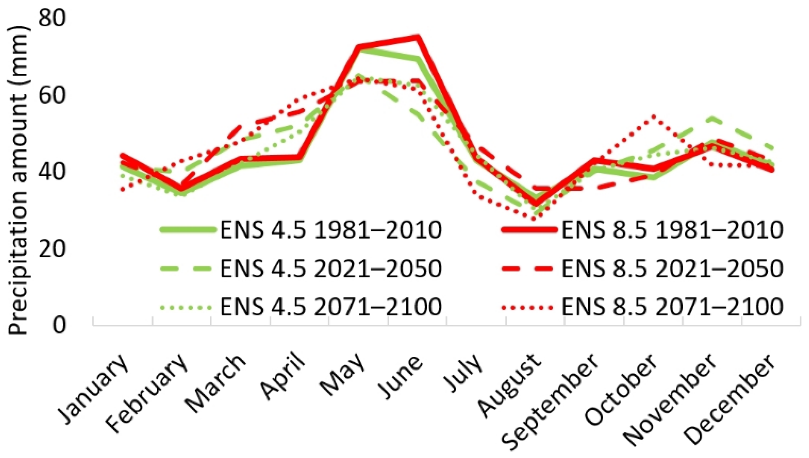
3.2. Climate Changes

The precipitation and temperature output from the climate models for both RCP 4.5 and RCP 8.5 together with several climate indicators are summarized in

Table 2. Average values for temperature, precipitation, and associated climate indicators for each climate model ensemble output for the reference, short- and long-term period (catchment scale).

	Absolute Values				Relative Change vs. Reference (%)
	Full Year		Growing Season		Full Year		Growing Season
Parameter	ENS RCP 4.5	ENS RCP 8.5	ENS RCP 4.5	ENS RCP 8.5	ENS RCP 4.5	ENS RCP 8.5	ENS RCP 4.5	ENS RCP 8.5
	1981–2010 (reference)
Precip. (mm/yr)	546.2	560.3	301.1	309.3
Ave. daily Tave. (°C)	10.8	10.8	18.3	18.3
Ave. daily Tmax. (°C)	16.0	15.9	24.1	24.0
Ave. daily Tmin. (°C)	5.9	5.8	12.5	12.4
Days with T < 0 °C (/yr)	98.2	98.7	3.2	3.4
Days with T > 25 °C (/yr)	84.6	83.2	83.4	81.8
Days with T > 35 °C (/yr)	5.1	5.2	5.1	5.2
Days with precip. (/yr)	163.5	164.6	78.2	78.9
	2021–2050 (short-term)
Precip. (mm/yr)	553.8	561.8	278.6	300.5	1.4	0.3	−7.5	−2.8
Ave. daily Tave. (°C)	12.0	12.1	19.6	19.6	11.0	12.4	6.8	7.2
Ave. daily Tmax. (°C)	17.2	17.2	25.3	25.2	7.1	8.2	5.1	5.2
Ave. daily Tmin. (°C)	7.1	7.2	13.7	13.7	20.5	23.2	9.7	10.6
Days with T < 0 °C (/yr)	85.2	83.7	2.7	2.0	−13.2	−15.1	−16.7	−40.3
Days with T > 25 °C (/yr 1)	101.2	100.1	98.9	97.1	19.6	20.3	18.6	18.8
Days with T > 35 °C (/yr)	10.3	9.7	10.3	9.7	103.5	87.8	103.5	87.3
Days with precip. (/yr)	159.8	159.6	72.2	74.9	−2.2	−3.1	−7.6	−5.1
	2071–2100 (long-term)
Precip. (mm/yr)	539.3	551.1	291.6	287.8	−1.3	−1.6	−3.1	−7.0
Ave. daily Tave. (°C)	13.1	15.0	20.5	22.5	20.7	39.8	11.6	23.0
Ave. daily Tmax. (°C)	18.3	20.2	26.1	28.1	14.0	27.2	8.6	17.0
Ave. daily Tmin. (°C)	8.1	10.1	14.6	16.7	38.0	73.2	17.1	34.4
Days with T < 0 °C (/yr)	70.6	48.2	0.9	0.4	−28.1	−51.1	−70.7	−88.2
Days with T > 25 °C (/yr)	109.5	129.4	106.4	123.8	29.4	55.5	27.6	51.4
Days with T > 35 °C (/yr)	14.6	27.2	14.6	27.2	189.0	425.1	189.0	424.9
Days with precip. (/yr)	156.5	148.7	73.7	69.2	−4.3	−9.7	−5.8	−12.3

,

Table 3. Monthly values for the representative year for average temperature and precipitation amount for each climate model ensemble output for the reference, short- and long-term period (catchment scale).

Parameter	ENS RCP 4.5
	1981–2010 (reference)
	Jan	Feb	Mar	Apr	May	Jun	Jul	Aug	Sep	Oct	Nov	Dec
Precip. (mm/yr)	41.4	34.5	41.5	43.0	71.9	69.3	42.9	33.2	40.7	38.5	47.6	41.8
Ave. daily Tave. (°C)	−1.7	−0.1	5.1	11.3	15.7	19.7	23.0	22.5	17.9	11.4	4.7	0.5
	2021–2050 (short-term)
	Jan	Feb	Mar	Apr	May	Jun	Jul	Aug	Sep	Oct	Nov	Dec
Precip. (mm/yr)	41.2	40.0	48.2	52.0	65.1	54.8 W	37.5	29.1	40.1	45.7	53.9	46.3
Ave. daily Tave. (°C)	−0.1	1.5	6.0	11.7	16.6	21.4	24.6	24.1	19.2	12.5	6.0	1.0
	2071–2100 (long-term)
	Jan	Feb	Mar	Apr	May	Jun	Jul	Aug	Sep	Oct	Nov	Dec
Precip. (mm/yr)	38.9	33.6	42.2	50.3	64.5	62.4	44.3	29.9	40.2	44.3	46.1	42.6
Ave. daily Tave. (°C)	1.0	2.8	8.1	12.9	17.6	21.9	25.3	25.0	20.1	13.3	6.6	2.2
	ENS RCP 8.5
	1981–2010 (reference)
	Jan	Feb	Mar	Apr	May	Jun	Jul	Aug	Sep	Oct	Nov	Dec
Precip. (mm/yr)	44.1	35.6	43.4	43.8	72.3	75.0	43.6	31.6	43.0	40.8	46.5	40.6
Ave. daily Tave. (°C)	−1.8	−0.2	5.2	11.2	15.7	19.6	22.8	22.6	17.7	11.4	4.5	0.6
	2021–2050 (short-term)
	Jan	Feb	Mar	Apr	May	Jun	Jul	Aug	Sep	Oct	Nov	Dec
Precip. (mm/yr)	42.4	36.5	51.8	55.4	63.4	63.7	46.7	35.6	35.7	39.0	48.6	43.0
Ave. daily Tave. (°C)	−0.9	2.0	6.5	12.1	16.8	21.2	24.3	23.8	19.1	13.1	6.0	1.1
	2071–2100 (long-term)
	Jan	Feb	Mar	Apr	May	Jun	Jul	Aug	Sep	Oct	Nov	Dec
Precip. (mm/yr)	35.4	42.8	47.7	58.9	64.2	61.3	33.8	27.4	42.1	54.2	41.7	41.5
Ave. daily Tave. (°C)	3.1	5.5	9.7	14.7	19.1	24.2	27.7	27.1	22.0	14.8	8.2	4.4

, Tables S2 and S3. When the annual averages are considered, the changes in precipitation amount for both the short (2021–2050) and long term (2071–2100) are insignificant when compared to the reference state (1981–2010) for both scenarios, representing less than ±2% for any given representative concentration pathway (RCP 4.5 and RCP 8.5). Compared to the reference period, both RCP 4.5 and RCP 8.5 showed an increase in monthly precipitation amounts between late winter and mid-spring, while the amounts of precipitation during the summer growing season (i.e., April–September) showed a consistent decrease (Table 3 and Table S3 and Figure 3). For RCP 4.5, the precipitation amount during the growing season will decrease by 7.5% over the short term and by 3.1% over the long term, while for RCP 8.5, it will decrease by 2.8% over the short term and by 7.0% over the long term. The number of days without precipitation will decrease overall, with a moderate impact of the two RCPs for the short term and a more pronounced impact for the long term. Thus, the decrease in the number of days with precipitation ranges from 2.2% for RCP 4.5 for the short term to 9.7% for RCP 8.5 for the long term. Similar to the precipitation amount, the relative changes (i.e., %) in the number of days without precipitation will be more pronounced during the growing season. These elements suggest that the anticipated future climate changes will result in a shift towards increased precipitation amounts outside of the growing season and a corresponding decrease during the growing season. This will likely result in additional stress on both agroecosystems and natural vegetation during the growing season, while outside of the growing season (e.g., spring), it could result in more significant peak flows and consequently increased risk and magnitude of flooding.

The changes were more pronounced with respect to the annual average temperature and ranged for the two RCPs from 11.0% to 12.4% for the short-term changes and from 20.7% to 39.8% for long-term changes (Table 2 and Table S2). The changes in average temperature during the growing season followed the same trend, but they were more moderate, representing about ~60% of the change in annual average temperature (Table 2 and Table 3). The increase for the two RCPs in minimum temperature is more significant than the corresponding increase in maximum daily temperature for both the short and long term. For the short term, the increase in average maximum temperature was relatively similar for the two RCPs (i.e., 7.1% for RCP 4.5 and 8.2 for RCP 8.5); however, the differences between the two trajectories became substantial for the long term (i.e., 14.0% for RCP 4.5 and 27.2% for RCP 8.5). The minimum daily temperature increased by 20.5% for RCP 4.5 and 23.2 for RCP 8.5 for the short term, while for the long term, it increased by 38.0% for RCP 4.5 and 73.2% for RCP 8.5. As it was the case with the average temperature, the minimum and maximum temperature had a more moderate increase during the growing season, with the changes representing only 40–50% of the change in annual average temperature (Table 2, Table 3, Tables S2 and S3). The other temperature-based climate indicators also showed significant changes. For example, the number of days with temperatures below 0 °C decreased by 13.2% (RCP 4.5) and 15.1% (RCP 8.5) for the short term, while for the long term, it decreased by 28.1% for RCP 4.5 and by more than half for RCP 8.5. Consequently, starting with the short-term period, the month of May became frost-free for both scenarios, while for the long-term period, the number of days with temperatures below the freezing point for the months of April and October dropped to less than one. Both the number of summer (Tmax > 25 °C) and hot (Tmax > 35 °C) days increased significantly for short and long term for both RCPs, with the increase in canicular days being more significant than the increase in summer days. The relative increase in the annual number of canicular days ranged from 103.5% (RCP 4.5) and 87.8% (RCP 8.5) for the short term to a staggering increase of 189% for RCP 4.5 and of 425% for RCP 8.5 for the long term.

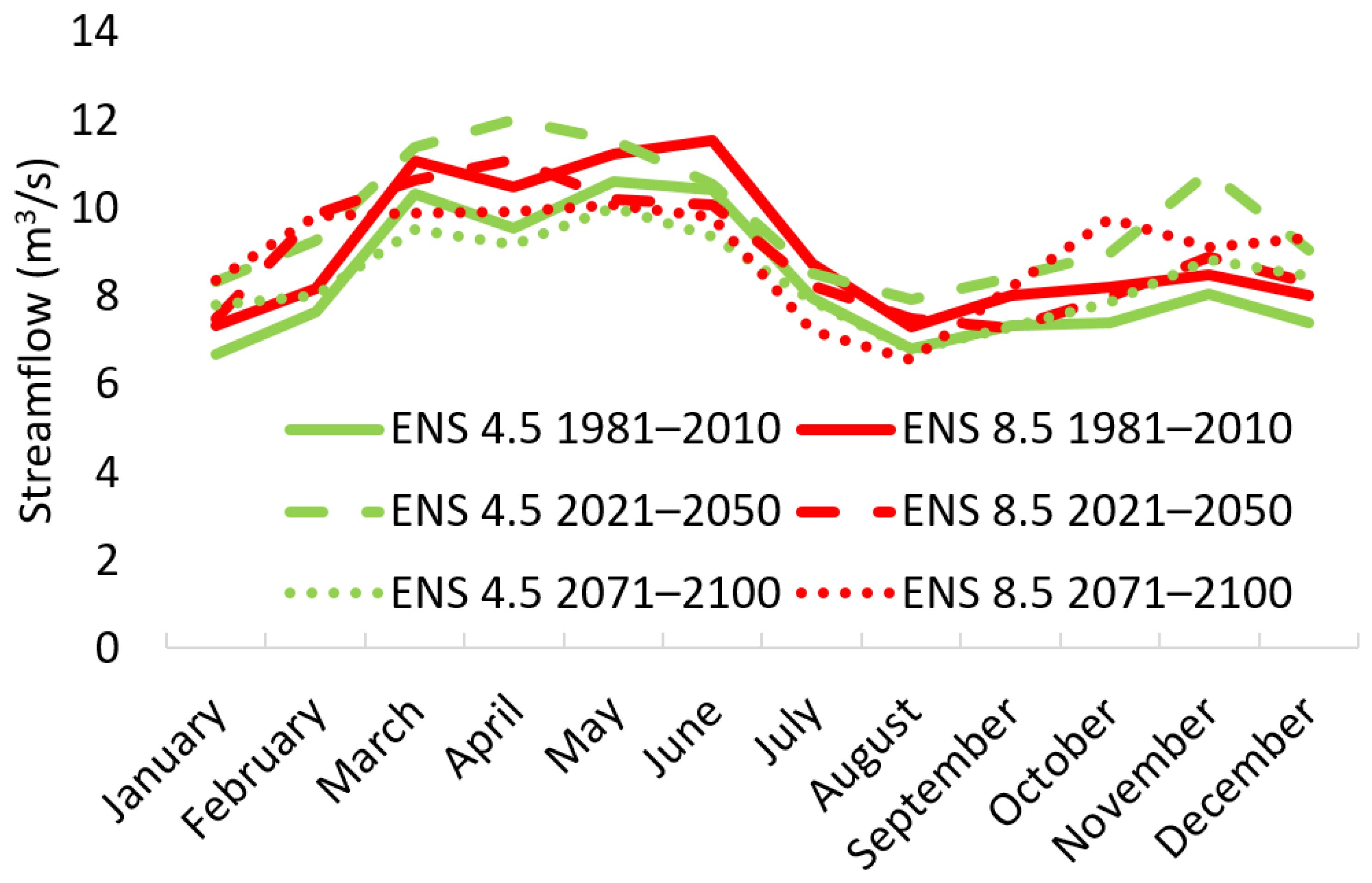
3.3. Water Balance Components (Temporal Dynamics)

The averages of the main water balance components resulted from SWAT simulations for each of the periods analyzed and RCP ensembles are shown in

Table 4. Average values for the main water balance components for the reference, short- and long-term periods (catchment scale) ¹.

Period	T	PP	SNMT	PET	ET	SW	PERC	SURF	LAT	Q
	°C	mm	mm	mm	mm	mm	mm	mm	mm	m3/s
	Full year multi-annual averages
	RCP 4.5
1981–2010	10.8	546.2	113.3	1150.8	455.4	81.5	47.9	5.4	33.1	8.3
2021–2050	12.0	553.8	113.8	1246.5	444.3	85.2	58.4	6.9	36.4	9.7
2071–2100	13.1	539.3	80.7	1296.0	449.0	79.2	46.8	5.0	34.5	8.4
	RCP 8.5
1981–2010	10.8	560.3	119.6	1138.8	460.9	84.4	54.5	5.7	23.3	9.0
2021–2050	12.1	561.8	104.4	1226.6	466.4	83.1	51.3	5.2	23.3	9.0
2071–2100	15.0	551.1	59.5	1410.5	455.0	80.5	51.9	4.9	22.0	9.0
	Growing season multi-annual averages
	RCP 4.5
1981–2010	18.3	301.1	8.2	929.1	352.7	77.7	22.1	3.6	17.3	8.8
2021–2050	19.6	278.6	11.6	1010.5	338.9	73.9	26.3	4.5	16.9	9.8
2071–2100	20.5	291.8	1.0	1034.1	340.4	66.6	17.0	3.3	16.0	8.4
	RCP 8.5
1981–2010	18.3	308.7	10.4	919.2	357.0	81.0	25.7	3.8	11.1	9.5
2021–2050	19.6	299.1	7.4	981.9	359.4	75.9	22.2	3.1	10.5	9.1
2071–2100	22.5	287.8	1.3	1116.1	337.5	63.6	19.3	2.7	8.9	8.6

Note: ¹ Legend: T—air temperature; PP—precipitation; SNMT—snowmelt; PET—potential; evapotranspiration; ET—actual evapotranspiration; SW—amount of water in soil; PERC—amount of water percolating out of root zone; SURF—surface runoff; LAT—lateral flow (mm); Q—streamflow (mm).

. For RCP 4.5, for the 2021–2050 period, the changes in snowmelt amount (SNMT), evapotranspiration (ET), and soil water content (SW) were minimal compared to the reference period (less than ±5%). However, changes in potential evapotranspiration (PET, +8.3%), percolation (PERC, +21.9%), surface runoff (SURF, +26.2%), and lateral flow (LAT, +10.0%) were more pronounced. The cumulative change for PERC, SURF, and LAT added up to 15.2 mm, which resulted from the slight increase in precipitation and the slight decrease in evapotranspiration. With respect to long-term (2071–2100) changes under RCP 4.5, the most significant changes were for SNMT, which decreased by 28.8% compared to the reference period, and for PET, which increased by 12.6%. For RCP 4.5, the flow at the outlet of the catchment increased significantly in the short term (Q, +16.6%), while in the long term, it had only a minimal increase (0.8%) compared to the reference period. Overall, these results suggest that for RCP 4.5, there will be more water available in the catchment in the short term, while in the long term, the amount available for streamflow will be similar to the reference period. For RCP 8.5 (Table 4), changes in water balance components are more significant than for RCP 4.5, with most water balance components decreasing for both sort- and long-term periods; however, ultimately, these changes resulted in minimal impacts on streamflow for both short- and long-term periods (i.e., −1.0% and 0.5%, respectively).

The monthly values of the main water balance components (Table S4) show that most components presented above will be impacted by future climate changes, regardless of the period of the analysis (i.e., short- or long-term) or RCP. However, it is expected that in some cases, the impacts on the ecosystem functioning will not be significant due to relatively small absolute values of the respective components. The impacts of the future climate changes will generally be more pronounced during the growing season (April–September; Table S4). Snowmelt (SNMT), which for the reference period had the highest amounts relatively uniformly distributed between January and March, will shift to December–February, with the monthly amount being reduced in some cases (e.g., 2071–2100, RCP 8.5) by more than 40%. These fundamental changes in the snowmelt process have a significant impact on soil water content (SW) in the catchment. Thus, for 2021–2050, SW will increase for both RCP 4.5 and RCP 8.5 between October and May, whereas between June and September, it will decrease by 10–30% for each month (Figure 4). The decrease in SW is accentuated for 2071–2100, with the period of reduced SW extending between March and September, and the decrease for each individual month reaching 35.5% in July for RCP 4.5 and 58% for the same month for RCP 8.5, respectively. Although the relative change in SW when the entire year is considered is less than ±5% for the various RCPs and future periods cases, it becomes more significant when the respective changes for the growing season are considered. For example, the SW for the growing season is expected to be reduced by 14.3% for RCP 4.5 and by 21.5% for RCP 8.5 over the long term compared to the reference state. Percolation to groundwater (PERC) is also significantly impacted by these changes, with most significant changes occurring for the long-term period, when for both RCP 4.5 and RCP 8.5, it will show the largest decrease between April and June and will increase between September and December. As it is the case with most water balance components, the most impact of the future climate changes on PERC will occur during the growing season. For example, for the long term, the relative change compared to the reference state for RCP 4.5 will be −2.8% when the entire year is considered, and −14.3% when only the growing season is considered. For the same period, under RCP 8.5, PERC is reduced by 4.7% when the entire year is considered, with the decrease during the growing season reaching −24.8%. Subsurface flow (LATQ) shows similar trends, including trend reversals when the full year and growing season averages for each period and RCP are compared. For example, for RCP 4.5 over the short term, LATQ shows a 10% increase when the full year is considered; however, during the growing season, LATQ will decrease by 1.8%. Similarly, for the long-term impacts of RCP 4.5, LATQ increases by 4.2% when the full year is considered, but it decreases by 7.1 when only the growing season is considered. For the most extreme case (i.e., long-term, RCP 8.5), the LATQ multi-annual yearly average decreases by 5.6%, while the growing season average decreases by 20.1%. These changes (e.g., SNMT, SW, PERC, LATQ) could have dramatic consequences on vegetative growth of both natural ecosystems and agroecosystems; for example, as the southern part of Romania currently is one of the areas with the highest withdrawal rate of water for agricultural purposes in the Danube catchment [51], the water resources in this region are already under stress [49,50], and this pressure is expected to increase in the future [24].

Streamflow (Q) also shows changes in the monthly dynamics. However, the pattern and magnitude of change vary depending on the RCP and period analyzed (Figure 5). For the short term, the SWAT output for RCP4.5 shows that Q will be higher for each month when compared to the reference period, with the smallest changes occurring between May and July. In several instances (e.g., January, February, April, October to December) the increase is more than 20%. Consequently, the increase in flow is more moderate for the growing season (i.e., 11.9%) than for the entire year (16.6%). This pattern is somewhat reversed for the long term, when between March and September, the streamflow decreased, by up to 10.4% in June. Consequently, the flow during the growing season shows a decrease of 4.2% compared to the reference state, although the flow slightly increases (i.e., 0.8%) when the entire year is considered. For RCP 8.5, the changes for the short term are less significant when compared to RCP 4.5 and also show a mix of months with increased and decreased streamflow. Thus, the streamflow between May and July decreases by up to 12.5% (June) when compared to the reference state and increases between November and February, showing a maximum increase in February (20.4%). With respect to short-term changes under RCP 8.5, the flow during the growing season decreases by 5.1% compared to the reference state, while it decreases only by 1.0% when the entire year is considered. The trends noted during the short term are accentuated during the long term, when the streamflow is decreasing between March and August, with all monthly reductions in flow being more than 10%, except for May (i.e., 5.5%). Under RCP 8.5, the changes to streamflow for the long term point to a decrease of 9.7% for the duration of the growing season, with an overall decrease of only 0.5% when the entire year is considered. The change in streamflow patterns during the growing season suggests that this would be a critical period in terms of availability of water (e.g., for irrigation or other uses, providing habitat for aquatic species, etc.), as in most cases, the anticipated impacts of climate changes will be more pronounced during this period. Outside of the growing season, the output from the various scenarios and periods suggests that generally there would be more water available, and hence, for example, during the spring, there could be an increased risk of flooding.

Comparison with other studies is challenging due to the range of time periods, climate models, and climate change scenarios used by the various authors. The lack of consistency in the prediction of the impacts on future climate changes on hydrological processes, as well as the uncertainty associated with the modeling of impacts of climate change in general has been recognized in the past by various authors as being the result of input data quality, selection of climate models, and the complex interactions between temperature, precipitation, and the hydrological process at the catchment scale [21,52,53]. Despite these limitations, the comparison of our results with the findings of other studies should be appropriate with respect to general trends. In addition, our study enriches the rather limited number of relevant studies conducted in this region of Europe. For example, Cuculeanu et al. (2002) [23] used a combination of five climate models to study the impacts of climate change up to 2070 and found similar results with our study relative to changes in snowfall and snowmelt patterns (i.e., shifting of the period with snowfall and the reduction in the amount of snowfall); however, they also found more drastic changes in precipitation patterns both for the cold (increase by ~20%) and the warm season (decrease by ~20%). Our results are also similar with the results presented by Cuculeanu et al. (2002) [23] with respect to soil water content, which will decrease, particularly during the growing season. Our findings are also similar in many respects to the results presented by Didovets et al. (2017) [21] for the Samara catchment located in eastern Ukraine. In the respective study, the impact of RCP 4.5 and RCP 8.5 on water resources was assessed for the near future (2011–2040), middle future (2041–2070), and far future (2071–2100) in three Ukrainian catchments using hydrological modeling. The Samara catchment is similar to the Neajlov catchment with respect to land use (75% cropland and 13% forest for Samara vs. 78% agricultural land and 10% forest for Neajlov), flow regime (i.e., high peak flows during spring and long streamflow recession and low flow during the summer and fall), average temperature (9.3 vs. 11.2 °C), and precipitation amount (589 vs. 525.7 mm), and also shows a similar range of future changes in temperature (+3.2 vs. 2.5 °C) and insignificant changes in annual precipitation amount (−20 mm), with an overall decrease in precipitation during the growing season for the long term, under the “intermediate” scenario. The results of the respective study suggest that the streamflow is expected to slightly increase over the near and middle-term future by 10–20% and decrease over the long term by ~10%, whereas in the Neajlov catchment, significant changes in streamflow are expected only under RCP 4.5 (i.e., increase for 2021–2050 and return to reference period values for 2071–2100), whereas the streamflow under RCP 8.5 remains relatively stable under all future time periods when the entire year is considered. However, both our study and that of Didovets et al. (2017) [21] are consistent with respect to the increased significance of climate changes during the growing season, when in both cases, a decrease in precipitation amount as well as streamflow is anticipated. Similar to the seasonal trends in Neajlov, the streamflow is expected to increase during the winter and spring season and decrease during the summer. Freund et al. (2017) [19] employed the SWAT model to evaluate potential impacts of future climate changes (2017–2050) on water resources in the Black Sea catchment using A2 and B2 IPCC scenarios combined with four land use change scenarios developed under the enviroGRIDS project [20]. While the range in temperature changes for the Neajlov area in the respective study is similar to the range presented in our study, the precipitation shows a more significant decrease (i.e., 5–15% depending on the scenario) compared to our study (i.e., 1.4% for RCP 4.5 and 0.3% for RCP 8.5) for this period and hence, it is difficult to directly compare the results of the two studies. However, the results of the respective study suggest that ET will decrease slightly (0–12%) for the Neajlov area, which is similar to our findings (i.e., −2.4% for RCP 4.5 and 1.2% for RCP 8.5), and conclude that areas of the Black Sea catchment, including Romania, will experience a decrease in water storage, which could lead to increased vulnerability with regard to freshwater resources.

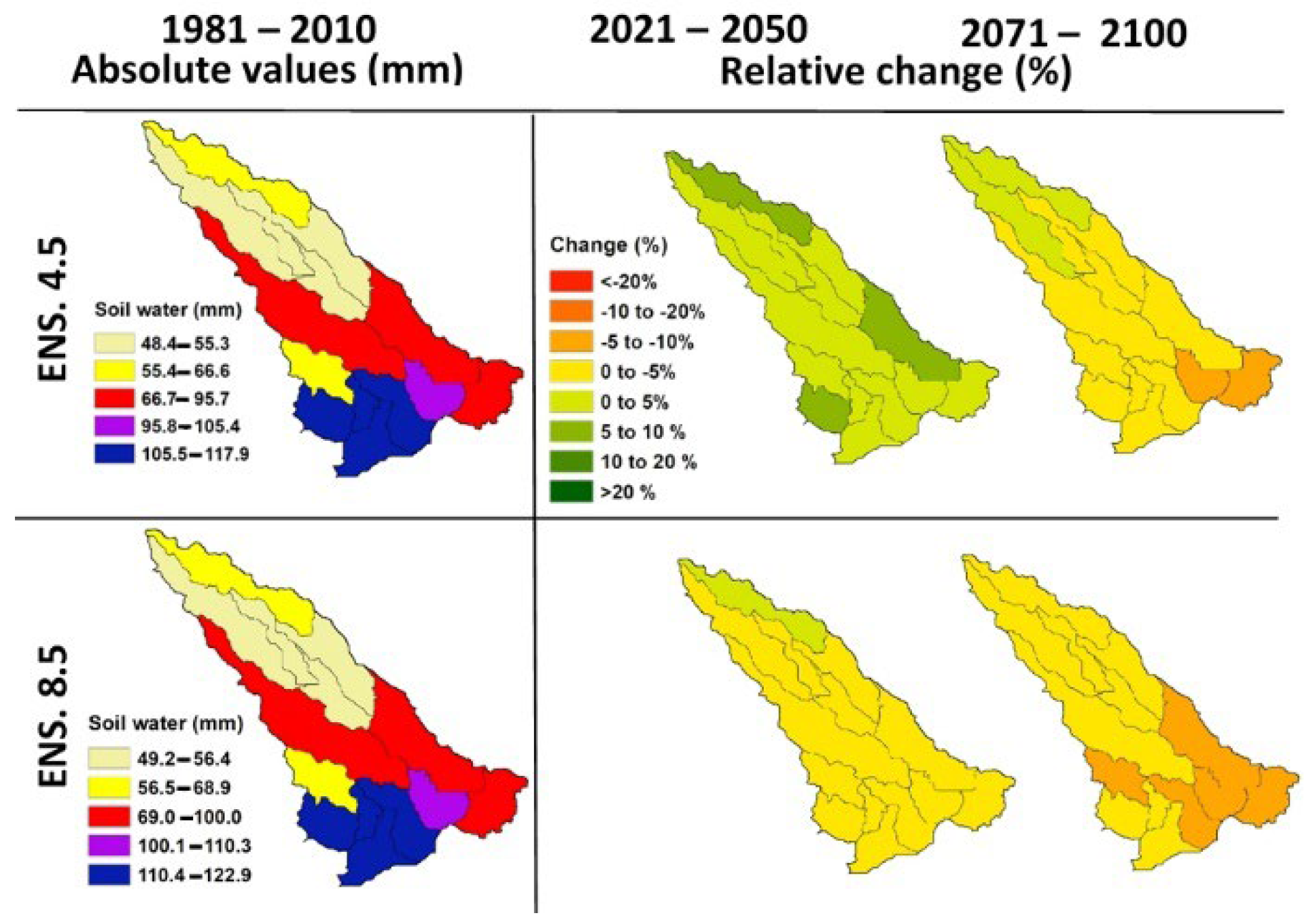
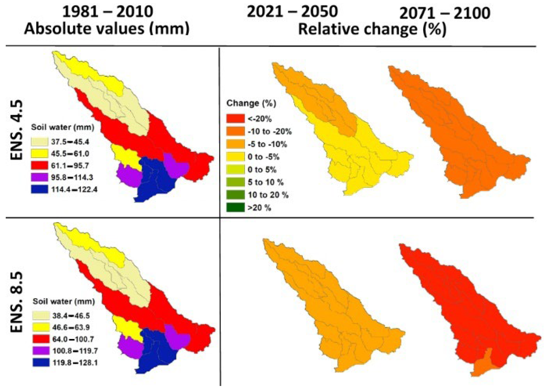
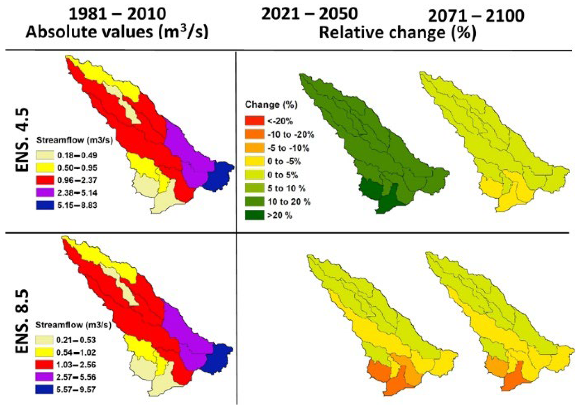
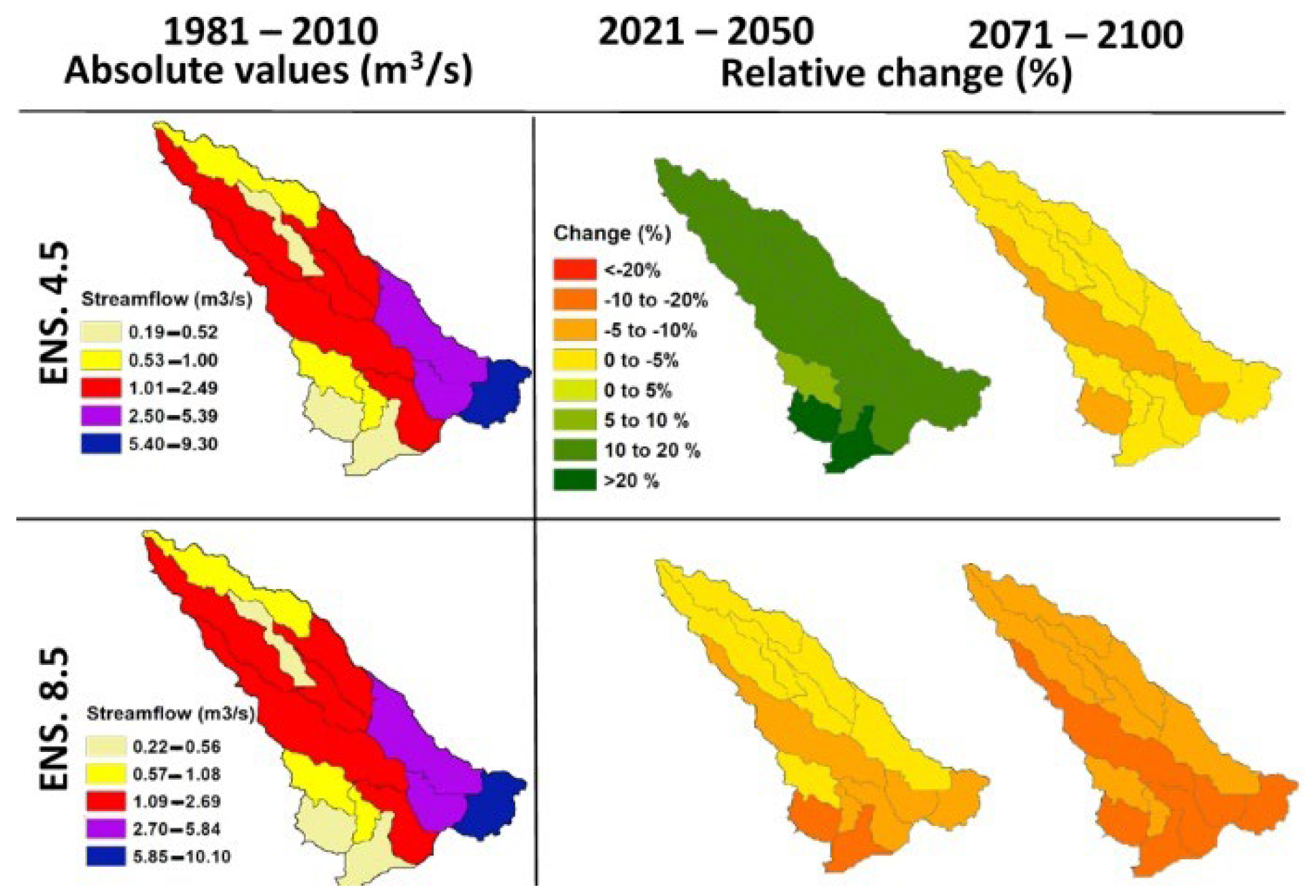
3.4. Water Balance Components (Spatial Patterns)

Despite the spatially uniform pattern of climate change, the spatial distribution of the average values for the water balance components RCP and period of analysis shows some heterogeneity at the catchment scale. The magnitude and direction of change vary depending on the RCP (i.e., 4.5 vs. 8.5) and period (i.e., short- vs. long-term; growing season vs. entire year) selected. The soil water content (SW) for RCP 4.5 during the short term will increase, but the changes are generally less than 5% and relatively uniformly distributed at the catchment scale, when the values for the entire year are considered (Figure 6). On the contrary, for the long term, the changes in SW result in drying of the soil (up to −5%), except for the upper portion of the catchment, where the soils still show an increase in SW (<5%). The most significant changes for the long term under RCP 4.5 are found in the lower portion of the catchment, which is also the portion that had the highest levels of SW during the reference period. The SW changes for RCP 8.5 show that most of the catchment over the short term and all the subcatchments over the long term will be drier by up to 10% compared to the reference state. The reduction in SW is widespread during the growing season (Figure 7), with RCP 8.5 showing more drastic changes than RCP 4.5 for both short- and long-term periods. Thus, SW under RCP 4.5 shows that about half of the catchment will experience a decrease of up to 5% in SW for the growing season, while for the other half of the catchment, SW will decrease by 5–10% over the short term. Over the long term, the SW for the entire catchment will decrease by 10–20% under RCP 4.5. RCP 8.5 shows more pronounced changes during the growing season, with SW decreasing by 5–10% for the short term and by more than 20% for the long term. Similar spatial trends are experienced by most of the water balance components (e.g., lateral flow; Figures S4 and S5). With respect to streamflow, except for the significant increase for the short term under RCP 4.5, stream discharge follows the same trends as SW, showing that the lower portions of the catchment are generally more sensitive to future changes. Thus, when the entire year is considered (Figure 8), most of the catchment will experience a relative increase in streamflow of up to 20% for the short-term, with two subcatchments in the lower portion of the catchment experiencing increases higher than 20%. For the long term, most of the catchment will experience an increase of up to 5% in streamflow. The results show more variability under RCP 8.5, when subcatchments will experience changes in streamflow ranging from −20% to 5% both for short- and long-term periods when considering the entire year. During the growing season (Figure 9), the increase under RCP 4.5 will be more moderate than for the entire year for the short term, while for the long term, all the catchments will experience a decrease in streamflow of up to 10%. For RCP 8.5, the streamflow will decrease during the growing season for all subcatchments, both for the short and long term, with decreases accentuated for the long term (i.e., up to 20% decrease for about half of the catchment). These findings suggest that the hydrological processes in the lower portions of the catchment are more sensitive to climate changes and hence, the heterogeneity of the impacts should be accounted for in the development of climate change adaptation strategies relative to water resources.

4. Conclusions

In this study, we used the output from three GCMs (CNRM, MPR, ICHEC) under two future climate projections (RCP 4.5 and RCP 8.5) in SWAT to understand the impacts of future climate changes on the hydrological process in the LTSER Neajlov River Catchment (3720 km² area), in the southeastern part of Romania, for short- (2021–2050) and long-term (2071–2100) changes. The anticipated changes in temperature and precipitation will have a more pronounced impact during the growing season, resulting in increased water stress (i.e., deficit) during this period. In addition, the results suggest that the hydrological processes in the lower portions of the catchment will be the most impacted by the future climate changes. This study contributes to advancing the understanding of climate change impacts on hydrological processes at the catchment scale, and to the best of our knowledge, this is the first study of this nature conducted in a Romanian catchment. Furthermore, the methodology involved in this study can be applied to other areas for assessing the impacts of climate changes on hydrological processes, as it provides support for formulating and implementing effective water resource management plans for minimizing the impact of future climate changes on water resources at the catchment scale. This study also provides the foundation for incorporating other factors such as land use and land cover changes in the assessment of impacts of future climate changes.

References

1. Intergovernmental Panel on Climate Change (IPCC). Contribution of Working Group I to the Sixth Assessment Report of the Intergovernmental Panel on Climate Change. In Climate Change 2021: The Physical Science Basis; Masson-Delmotte, V., Zhai, P., Pirani, A., Connors, S.L., Péan, C., Berger, S., Caud, N., Chen, Y., Goldfarb, L., Gomis, M.I., et al., Eds.; Cambridge University Press: Cambridge, UK, 2021. [Google Scholar]
2. Dayon, G.; Boé, J.; Martin, E.; Gailhard, J. Impacts of climate change on the hydrological cycle over France and associated uncertainties. Comptes Rendus Geosci. 2018, 350, 141–153. [Google Scholar] [CrossRef]
3. Dawen, Y.; Yang, Y.; Xia, J. Hydrological cycle and water resources in a changing world: A review. Geog. Sust. 2021, 2, 115–122. [Google Scholar] [CrossRef]
4. Heino, R.; Brazdil, R.; Forland, E.; Tuomenvirta, H.; Alexandersson, H.; Beniston, M.; Pfister, C.; Rebetez, M.; Rosenhagen, G.; Rosner, S.; et al. Progress in the study of climatic extremes in northern and central Europe. Clim. Change 1999, 42, 151–181. [Google Scholar] [CrossRef] [Green Version]
5. Boorman, D.B. Climate, Hydrochemistry and Economics of Surface-water Systems (CHESS): Adding a European dimension to the catchment modelling experience developed under LOIS. Sci. Total Environ. 2003, 314, 411–437. [Google Scholar] [CrossRef]
6. Kovats, R.S.; Valentini, R.; Bouwer, L.M.; Georgopoulou, E.; Jacob, D.; Martin, E.; Rounsevell, M.; Soussana, J.-F. Part B: Regional Aspects. Chapter 23: Europe. Contribution of Working Group II to the Fifth Assessment Report of the Intergovernmental Panel on Climate Change. Europe. In Climate Change 2014: Impacts, Adaptation, and Vulnerability; Barros, V.R., Field, C.B., Dokken, D.J., Mastrandrea, M.D., Mach, K.J., Bilir, T.E., Chatterjee, M., Ebi, K.L., Estrada, Y.O., Genova, R.C., et al., Eds.; Cambridge University Press: Cambridge, UK, 2014; pp. 1267–1326. [Google Scholar]
7. European Environment Agency (EEA). EEA Report 1/2017. In Climate Change, Impacts and Vulnerability in Europe 2016: An Indicator-Based Report; European Environment Agency: Copenhagen, Denmark, 2017; Available online: https://www.eea.europa.eu/publications/climate-change-impacts-and-vulnerability-2016 (accessed on 21 September 2020).
8. Howarth, C.; Painter, J. Exploring the science–policy interface on climate change: The role of the IPCC in informing local decision-making in the UK. Palgrave Comm. 2016, 2, 16058. [Google Scholar] [CrossRef] [Green Version]
9. Singh, V.P. Hydrologic modeling: Progress and future directions. Geosci. Lett. 2018, 5, 15. [Google Scholar] [CrossRef]
10. Fadeyi, O.; Maresova, P. Stakeholders’ Perception of Climate Actions in Some Developing Economies. Climate 2020, 8, 66. [Google Scholar] [CrossRef]
11. Beek, T.A.; Kynast, E.; Flörke, M. Modelling Current and Future Pan-European Irrigation Water Demands and Their Impact on Water Resources. In Problems, Perspectives and Challenges of Agricultural Water Management; Kumar, M., Ed.; IntechOpen: London, UK, 2012; p. 427. ISBN 978-953-51-0117-8. Available online: https://www.intechopen.com/chapters/31500 (accessed on 10 August 2021).
12. Greuell, W.; Andersson, J.C.M.; Donnelly, C.; Feyen, L.; Gerten, D.; Ludwig, F.; Pisacane, G.; Roudier, P.; Schaphoff, S. Evaluation of five hydrological models across Europe and their suitability for making projections under climate change. Hydrol. Earth Syst. Sci. Discuss. 2015, 12, 10289–10330. [Google Scholar] [CrossRef]
13. Donnelly, C.; Greuel, W.; Andersson, J.; Gerten, D.; Pisacane, G.; Roudier, P.; Ludwig, F. Impacts of climate change on European hydrology at 1.5, 2 and 3 degrees mean global warming above preindustrial level. Clim. Change 2017, 143, 13–26. [Google Scholar] [CrossRef] [Green Version]
14. Gudmundsson, L.; Wagener, T.; Tallaksen, L.M.; Engeland, K. Evaluation of nine large-scale hydrological models with respect to the seasonal runoff climatology in Europe. Water Resour. Res. 2012, 48, W11504. [Google Scholar] [CrossRef]
15. Sood, A.; Smakhtin, V. Global hydrological models: A review. Hydrol. Sci. J. 2015, 60, 549–565. [Google Scholar] [CrossRef]
16. Bar, R.; Rouholahnejad, E.; Rahman, K.; Abbaspour, K.C.; Lehmann, A. Climate change and agricultural water resources: A vulnerability assessment of the Black Sea catchment. Env. Sci. Pol. 2015, 47, 57–69. [Google Scholar] [CrossRef]
17. Verzano, K. Climate Change Impacts on Flood Related Hydrological Processes: Further Development and Application of a Global Scale Hydrological Model. Ph.D. Thesis, University of Kassel, Kassel, Germany, 2009. Available online: https://pure.mpg.de/pubman/item/item_993926_5/component/file_993925/WEB_BzE_71.pdf (accessed on 15 October 2021).
18. Intergovernmental Panel on Climate Change (IPCC). Contribution of Working Group I to the Fourth Assessment Report of the Intergovernmental Panel on Climate Change. In Climate Change 2007: The Physical Science Basis; Alley, R.B., Allison, I., Carrasco, J., Falto, G., Fujii, Y., Kaser, G., Mote, P., Thomas, R.H., Zhang, T., Eds.; Cambridge University Press: Cambridge, UK, 2007. [Google Scholar]
19. Freund, E.R.; Abbaspour, K.C.; Lehman, A. Water Resources of the Black Sea Catchment under Future Climate and Landuse Change Projections. Water 2017, 9, 598. [Google Scholar] [CrossRef] [Green Version]
20. Lehmann, A.; Giuliani, G.; Mancosu, E.; Abbaspour, K.C.; Sözen, S.; Gorgan, D.; Beel, A.; Ray, N. Filling the gap between Earth observation and policy making in the Black Sea catchment with enviroGRIDS. Environ. Sci. Policy 2015, 46, 1–12. [Google Scholar] [CrossRef]
21. Didovets, I.; Lobanova, A.; Bronstert, A.; Snizhko, S.; Maule, C.F.; Krysanova, V. Assessment of Climate Change Impacts on Water Resources in Three Representative Ukrainian Catchments Using Eco-Hydrological Modelling. Water 2017, 9, 204. [Google Scholar] [CrossRef] [Green Version]
22. Krysanova, V.; Wechsung, F.; Arnold, J.; Ragavan, S.; Williams, J. PIK Report No. 69. In SWIM (Soil and Water Integrated Model), User Manual; Potsdam Institute for Climate Impact Research: Potsdam, Germany, 2000. [Google Scholar]
23. Cuculeanu, V.; Tuinea, P.; Bǎlteanu, D. Climate change impacts in Romania: Vulnerability and adaptation options. GeoJournal 2002, 57, 203–209. [Google Scholar] [CrossRef]
24. Mitrică, B.; Bogardi, I.; Mitrică, E.; Mocanu, I.; Minciună, M. A forecast of public water scarcity on Leu-Rotunda Plain, Romania, for the end of the 21st century. Nor. Geogr. Tidsskr. Nor. J. Geo. 2017, 71, 12–29. [Google Scholar] [CrossRef]
25. Arnold, J.G.; Kiniry, J.R.; Srinivasan, R.; Williams, J.R.; Haney, E.B.; Neitsch, S.L. Soil & Water Assessment Tool: Input/Output Documentation; Version 2012; TR-439; Texas Water Resources Institute: College Station, TX, USA, 2012; pp. 1–650. [Google Scholar]
26. Dosio, A. EU High Resolution Temperature and Precipitation Dataset. European Commission, Joint Research Centre (JRC), 2018, PID. Available online: http://data.europa.eu/89h/jrc-liscoast-10011 (accessed on 17 May 2020).
27. Fetting, C. The European Green Deal, ESDN Report, December 2020; ESDN Office: Vienna, Austria, 2020. [Google Scholar]
28. United Nations Climate Change (UNCC). Annual Report 2020; ISBN 978-92-9219-197-9. Available online: https://unfccc.int/annualreport (accessed on 19 December 2021).
29. Mirtl, M.; Orenstein, D.E.; Wildenberg, M.; Peterseil, J.; Frenzel, M. Development of LTSER platforms in LTER-Europe: Challenges and experiences in implementing place-based long-term socio-ecological research in selected regions. In Long Term Socio-Ecological Research; Singh, S.J., Haberl, H., Chertow, M., Mirtl, M., Schmid, M., Eds.; Springer: Dordrecht, The Netherlands, 2013; pp. 409–442. [Google Scholar]
30. Pişota, I.; Cocoş, O. Unele observaţii hidrologice referitoare la bazinul râului Neajlov. Comunicări De Geografie. 2003, 7, 183–188. (In Romanian) [Google Scholar]
31. National Institute for Hydrology and Water Management (NIHWM). Daily Measured Discharge at Moara din Groapa, Vadu Lat and Calugareni Stations (1981–2010). 2020. Available online: https://www.un-igrac.org/donor-partner/nihwm (accessed on 25 May 2020).
32. Grecu, F.; Ghita, C.; Albu, M.; Circiumaru, E. Geomorphometric analysis on some riverbeds in the Romanian plain. Int. J. Phys. Sci. 2011, 30, 7055. [Google Scholar] [CrossRef]
33. Agentia Nationala de Protectie a Mediului (ANPM). Rapport Judetean Privind Starea Mediului—Judetul Arges. Starea Calitatii Apei in Judetul Arges pe Anul 2014. Ministerul Mediului; ANPM Arges: Pitești, Romania, 2014; p. 67. (In Romanian) [Google Scholar]
34. FAO/UNESCO/ISRIC. FAO/UNESCO Soil Map of the World; Revised Legend, with corrections and updates. World Soil Resources Report 60; Reprinted with updates as Technical Paper 20; FAO: Rome, Italy; ISRIC: Wageningen, The Netherlands, 1997; ISBN 92-5-103022-7. Available online: https://www.fao.org/fileadmin/user_upload/soils/docs/isricu_i9264_001.pdf (accessed on 2 March 2022).
35. National Meteorological Administration (NMA). Daily Meteorological Data for Videle Station (1981–2010). 2020. Available online: https://weamyl.met.no/anm/ (accessed on 25 May 2020).
36. Winchell, M.; Srinivasan, R.; Di Luzio, M.; Arnold, J. ArcSWAT interface for SWAT 2012—User’s Guide; Blackland Research and Extension Centre, Texas AgriLife Research and Grassland, Soil and Water Research Laboratory, USDA Agricultural Research Service: Temple, TX, USA, 2013; p. 464. [Google Scholar]
37. Blaschke, A.; Schilling, C. daNUbs—Report “Water Balance Calculations for the Case Study Regions in Austria, Hungary and Romania”; Institute of Hydraulics, Hydrology and Water Resources Management: Vienna, Austria; Vienna University of Technology: Vienna, Austria, 2003; p. 155. Available online: https://iwr.tuwien.ac.at/wasser/forschung/projekte/projektarchiv/danubs/ (accessed on 20 May 2021).
38. European Environment Agency (EEA). Copernicus Land Service (CLC)-Pan-European Component: CORINE Land Cover. 2012. Available online: https://www.eea.europa.eu/data-and-maps/data/copernicus-land-monitoring-service-corine (accessed on 23 May 2018).
39. Abbaspour, K.C. SWAT-CUP Premium: SWAT Calibration and Uncertainty Programs—A User Manual; Water, Weather Energy, and Ecosystem Technology and Data (2W2E): Zurich, Switzerland, 2020; p. 7. [Google Scholar]
40. Arnold, J.G.; Moriasi, D.N.; Gassman, P.W.; Abbaspour, K.C.; White, M.J.; Srinivasan, R.; Santhi, C.; Harmel, R.D.; van Griensven, A.; Van Liew, M.W.; et al. SWAT: Model use, calibration and validation. Trans. ASABE 2012, 55, 1491–1508. [Google Scholar] [CrossRef]
41. Abbaspour, K.C.; Rouholahnejad, E.; Vaghefi, S.; Srinivasan, R.; Yang, H.; Klove, B. A continental-scale hydrology and water quality model for Europe: Calibration and uncertainty of a high-resolution large-scale SWAT model. J. Hydrol. 2015, 524, 733–752. [Google Scholar] [CrossRef] [Green Version]
42. Abbaspour, K.C.; Vaghefi, S.A.; Srinivasan, R. A Guideline for Successful Calibration and Uncertainty Analysis for Soil and Water Assessment: A Review of Papers from the 2016 International SWAT Conference 2. Water 2018, 10, 6. [Google Scholar] [CrossRef] [Green Version]
43. Nash, J.E.; Sutcliffe, J.V. River flow forecasting through conceptual models—Part 1: A discussiojn of principles. J. Hydrol. 1970, 82, 290. [Google Scholar] [CrossRef]
44. Stefanidis, S.P. Ability of different spatial resolution regional climate models to simulate air temperature in a forest ecosystem of central Greece. J. Environ. Prot. Ecol. 2021, 22, 1488–1495. [Google Scholar]
45. Busuioc, A.; Dumitrescu, A.; Baciu, M.; Cazacioc, L.; Cheval, S. RCM performance in reproducing temperature and precipitation regime in Romania. Application for Banat Plain and Oltenia Plain. Rom. J. Meteorol. 2010, 10, 19. [Google Scholar]
46. Spruill, C.A.; Workman, S.R.; Taraba, J.L. Simulation of daily and monthly stream discharge from small watersheds using the SWAT Model. Trans. ASABE 2000, 43, 1431–1439. [Google Scholar] [CrossRef]
47. Ahl, R.S.; Woods, S.W.; Zuuring, H.R. Hydrologic Calibration and Validation of SWAT in a Snow-Dominated Rocky Mountain Watershed, Montana, USA. J. Am. Water Resour. Assoc. 2008, 44, 1411–1430. [Google Scholar] [CrossRef]
48. Remesan, R.; Bellerby, T.; Frostick, L. Hydrological modelling using data from monthly GCMs in a regional catchment. Hydrol. Process. 2014, 28, 3241–3263. [Google Scholar] [CrossRef] [Green Version]
49. Guteascu, M.; Constantinescu, T.; Cracuin, S.; Bascoveanu, D.; Podoleanu, D. Deliverable to Task A3 of the BLUE 2 project “Study on EU integrated policy assessment for the freshwater and marine environment, on the economic benefits of EU water policy and on the costs of its non- implementation”. In Annex VII. Application of the Bottom-Up Multicriteria Methodology in Eight European River Basin Districts—The Arges-Vedea RBD; Ramboll Group A/S: Copenhagen, Denmark, 2018; p. 70. [Google Scholar]
50. Administratia Nationala Apele Romane (ANAR). Proiectul planului de management actualizat (2021) afferent portiunii nationale a bazinului hidrografic international al fluviului Dunarea. Sinteza proiectelor planurilor de management actualizate la nivel de bazine/spatii hidrogtrafice. Ministerul Mediului, Apelor si Padurilor: Bucuresti, Romania, 2021; p. 411. (In Romanian). Available online: https://weamyl.met.no/anm/ (accessed on 25 May 2020).
51. Karabulut, A.; Egoh, B.N.; Lanzanova, D.; Grizzetti, B.; Bidoglio, G.; Pagliero, L.; Bouraoui, F.; Aloe, A.; Reynaud, A.; Maes, J.; et al. Mapping water provisioning services to support the ecosystem–water–food–energy nexus in the Danube river basin. Ecosyst. Serv. 2015, 17, 278–292. [Google Scholar] [CrossRef]
52. Cerkasova, N.; Umgiesser, G.; Ertürk, A. Development of a hydrology and water quality model for a large transboundary river watershed to investigate the impacts of climate change—A SWAT application. Ecol. Eng. 2018, 124, 99–115. [Google Scholar] [CrossRef]
53. Kiesel, J.; Gericke, A.; Rathjens, H.; Wetzig, A.; Kakouei, K.; Jähnig, S.C.; Fohrer, N. Climate change impacts on ecologically relevant hydrological indicators in three catchments in three European ecoregions. Ecol. Eng. 2019, 127, 404–416. [Google Scholar] [CrossRef]
Figure 1. Neajlov River main tributaries, subcatchments (1–14), including stream and meteorological monitoring stations. Inset: Location of Neajlov catchment in Romania.
Water 14 02325 g001
Figure 2. Spatial distribution of soil (a) and land use (b) types in the Neajlov River Catchment.
Water 14 02325 g002
Figure 3. Precipitation amount for the representative monthly year for each climate model output for the reference, short- and long-term period.
Water 14 02325 g003
Figure 4. Soil water content for the representative monthly year for each climate model output for the reference, short- and long-term periods.
Water 14 02325 g004
Figure 5. Streamflow at the catchment outlet for the representative monthly year for each climate model output for the reference, short- and long-term periods.
Water 14 02325 g005
Figure 6. Catchment-scale distribution of annual average soil water content (SW) for the reference period (mm) and the relative change compared to the reference period (%) for each RCP.
Water 14 02325 g006
Figure 7. Catchment-scale distribution of growing season average soil water content (SW) for the reference period (mm) and the relative change compared to the reference period (%) for each RCP.
Water 14 02325 g007
Figure 8. Catchment-scale distribution of annual average streamflow for the reference period (mm) and the relative change compared to the reference period (%) for each RCP.
Water 14 02325 g008
Figure 9. Catchment-scale distribution of growing season average streamflow for the reference period (mm) and the relative change compared to the reference period (%) for each RCP.
Water 14 02325 g009