
Smart Sharing Plan: The Key to the Water Crisis

1
School of Information Engineering, China University of Geosciences (Beijing), Beijing 100083, China
2
School of Science, China University of Geosciences (Beijing), Beijing 100083, China
*
Author to whom correspondence should be addressed.
Water 2022, 14(15), 2320; https://doi.org/10.3390/w14152320
Submission received: 14 June 2022
/
Revised: 20 July 2022
/
Accepted: 22 July 2022
/
Published: 26 July 2022
(This article belongs to the Special Issue Water Scarcity: From Ancient to Modern Times and the Future)
Abstract
:Over the years, the Colorado River has become inadequate for development due to natural factors and human activities. The hydroelectric facilities in Lake Mead and Lake Powell are also not fully utilized. Downstream, Mexico is also involved in the competition for water. The resulting allocation of water and electricity resources and sustainable development are hanging over our heads and waiting to be solved. In this work, a simplified Penstock Dam model and a Distance Decay model are designed based on publicly available data, and a Multi-attribute Decision model for hydropower based on the Novel Technique for Order Preference by Similarity to an Ideal Solution method is proposed. In addition, an Improved Particle Swarm Optimization model is proposed by adding oscillation parameters. The Mexican equity problem is also explored. The theoretical results show that the average error of the Penstock Dam model is 3.2%. The minimum water elevation requirements for Lake Mead and Lake Powell are 950 ft and 3460 ft, respectively; they will not meet demand in 2026 and 2027 without action, and they will require the introduction of and water in 2027 and 2028, respectively. The solution shows that the net profit for the United States is greatest when 38.6% of the additional water is used for general purposes, 47.5% is used for power generation, and the rest flows to Mexico. A final outlook on the sustainability of the Colorado River is provided.
1. Introduction
Hydropower generation is a major part of the power industry and has made great contributions to the progress of world civilization [1]. Most obviously, hydropower solves many energy supply problems [2]. It provides pollution-free renewable energy [3], which is only a reasonable absorption of natural energy by human beings, basically free of pollutants, and realizes the organic combination of industrial progress and environmental protection [4].
Hydropower generation not only can obtain renewable and clean energy, but can also start and stop quickly, adjust the load, and perform peaking, frequency regulation, and accident backup in the power grid [5]. The construction of modern hydropower plants is taking on a wider range of tasks, increasingly enhancing the effectiveness of water resources allocation, disaster and drought mitigation, environmental and ecological improvement, and tourism [6].
In 1935, the Tennessee Valley Authority built the 2214.4 m high Hoover Dam (HD) on Lake Mead (LM) in the southwest of the United States [7], with a capacity of 35.2 billion m3. In 1957, the 216-m-high Glen Canyon Dam (GCD) was built upstream of HD and is managed by the U.S. military [8]. The GCD impounds water to form Lake Powell (LP), a valuable water resource for the surrounding arid region and a famous tourist area.
GCD and HD have made significant contributions to hydropower generation, flood storage, irrigation, and tourism [9]. However, according to the U.S. Bureau of Reclamation and the U.S. Geological Survey, by now, LM’s water volume accounted for only 35% of its capacity, while LP’s accounted for 31%, and the storage capacity of each reservoir in the entire basin is only 40% of the reservoir capacity. The water level of LM and its upper reaches of LP has been in a continuous downward trend since 2000 [10]. The main causes of the imbalance between supply and demand include poor planning of water allocation, rapid population growth, and global warming [11].
The base of hydropower generation must be a high mountain and deep river area [2], and it must be the storage place of mineral resources and the habitat of some special organisms or biological species [12], and most of them are the magnificent and exotic scenery of nature, so it must be a complicated area with intertwined conflicts. It involves not only the problem of electricity, but also the problem of water storage and supply [13]. This is also a major problem facing the United States at present.
The Colorado River (CR) has more than 25 tributaries, of which the upper Gunnison, Green, and San Juan rivers contribute nearly 11 cubic kilometers of water to the CR each year. All tributaries form the CR Basin, which covers 640,000 square kilometers and spans seven U.S. states and Mexico [14]. The water supply agreement involving the seven States of the CR Basin states and Mexico was signed nearly 100 years ago [15,16], during the historical flood period, and the agreement is based on runoff data that differ significantly from today [17,18]. It poses not only the challenge of water scarcity, but even the problem of pollution caused by less water [19]. It has been pointed out that the current U.S. government’s management of the ecosystem, including water management, lags behind demand, and climate change “constantly reminds people that this system is a poorly designed system, and our management is not well thought out” [20]. According to the data, the past 20 years have been the most significant period of declining water levels in the two reservoirs, with LM losing more than 2 billion cubic meters of stored water over the past 20 years, equivalent to 800,000 standard 2-m-deep swimming pools. The U.S. Bureau of Reclamation had declared LM to be in the first level water shortage status from 2022. The United States needs to do more to avoid a bigger catastrophe.
The lack of water can also bring about a drop in water levels, which affects the amount of hydroelectricity generated and has an impact on the city’s power supply [21,22]. Therefore, it is essential to consider how to optimize a rational, defensible water allocation plan for current and future water supply after taking into account the water demands of states and the conflicts of interest among them [4,23].
Mathematical modeling is an important tool for solving water supply and demand problems at dams and for deploying water resources [24,25]. First, it is important to fully deploy hydropower resources in the face of limited environmental conditions. Dominique M. Bain et al. quantified the value of hydropower in the operation of the CR power system, examining the value of hydropower and the cost of power under different possible future drought conditions and regional generation scenarios [26]. Benjamin A. Jones et al. studied the hydropower operating model in the basin in a referendum format [27]. Mort Webster et al. analyzed the effects of climate on electricity demand and costs, modeling them in terms of hydrology, power system, and economic levels [28]. For water allocation issues, Niklas S. Christensen et al. analyzed the effects of climate change on hydrology and water resources in the CR Basin [20]. William Chen et al. addressed dams to regulate human and environmental water demand in rivers by designing water flows [13]. Projections of hydropower and water resources are also important tools to address this challenge. Syed Azhar Ali et al. predicted the increase of hydropower resources in India in the context of climate change [29]. Chikamoto et al. predicted the water flow of the CR from the perspective of ocean memory [23].
In addition, the historical issue of competition between the United States and Mexico for CR water resources cannot be ignored, and how to allocate water resources to adequately meet the needs of both peoples is an important research question [30,31].
From the above presentation, it is clear that if a series of mathematical models can be developed that can adequately balance the water and hydropower needs around the watershed, and if these models can effectively contribute to sustainable development, they will have a positive impact on the future of the world’s watersheds, including the CR. This work is based on the five major states with severe water shortages radiating from the middle and lower CR. We have prepared a theoretically sound mathematical solution for water and hydropower resource planning and sustainable development.
This work starts from the basic electricity and water demands of the area under discussion, and fully analyzes the conditions for the healthy operation of the two dams and the lake in which they are located by simplifying the dam generation model, optimizing the water and hydropower distribution model, and considering multiple factors together. The article predicts their service life under extreme conditions and without management action. The paper focuses on the sustainable development of the southwestern United States, including the issue of Mexican rights, at the policy level after a rational analysis. The work also presents a sensitivity analysis of the model developed to explore its generalizability. It concludes with a brief evaluation of the work and suggests ideas for further improvement. We use data and analysis as evidence to explore conservation and development. This work will also demonstrate the broad applicability of our model, to explore water issues more deeply.
Researchers tend to focus on a single perspective on water allocation issues, as illustrated in the previous section. Researchers have chosen their areas of expertise as entry points for in-depth research. A series of studies have provided climate and geographic perspectives on the future development of the CR. Remote sensing images have been borrowed to analyze water evapotranspiration in the CR basin [32]. A more granular perspective is being used for agricultural water use. Hung et al. examined uncertainties at the system, agent, and parameter levels through uncertainty, clustering, and sensitivity analyses. In their model, CR would face a 13 to 30 year-long water crisis between 2019 and 2060 [33]. Other studies examine the allocation of CR water resources from market and policy perspectives [34,35,36]. Most of these studies are based on historical facts and market context.
Relatively speaking, the value of our work is in a sense comprehensive and forward-looking. This work adequately addresses water and hydropower needs, taking into account all factors in order to develop a relatively complete and idealized mathematical model. The mathematical model is used to guide policy implementation in a scientifically sound manner. At the same time, the work focuses on the actual water crisis of the people of the five states from both historical and practical perspectives, proposing minimum water requirements of 950 feet and 3460 feet for LM and LP, respectively. The work also warns that if no action is taken, LM and LP will not be able to meet demand in 2026 and 2027, respectively. The need for timely action is also well documented by relevant data type studies [18]. This work specifies diversions and proportional allocations, including residential, agricultural, and industrial water, with full consideration of the interests of the Mexican downstream of the CR, providing specific followings for historical dilemmas and sustainable development of the CR.
The guiding allocation scheme we propose addresses the real water crisis problem head on, and the scientific validity of the model predictions is fully demonstrated in the paper. The problem of water allocation involving the CR, including the country of Mexico, is historical in nature. Addressing it from a mathematical modeling perspective and complementing it with argumentation is novel and reliable. Our quantitative and qualitative analyses are of great value and provide guidance for subsequent studies involving this area.
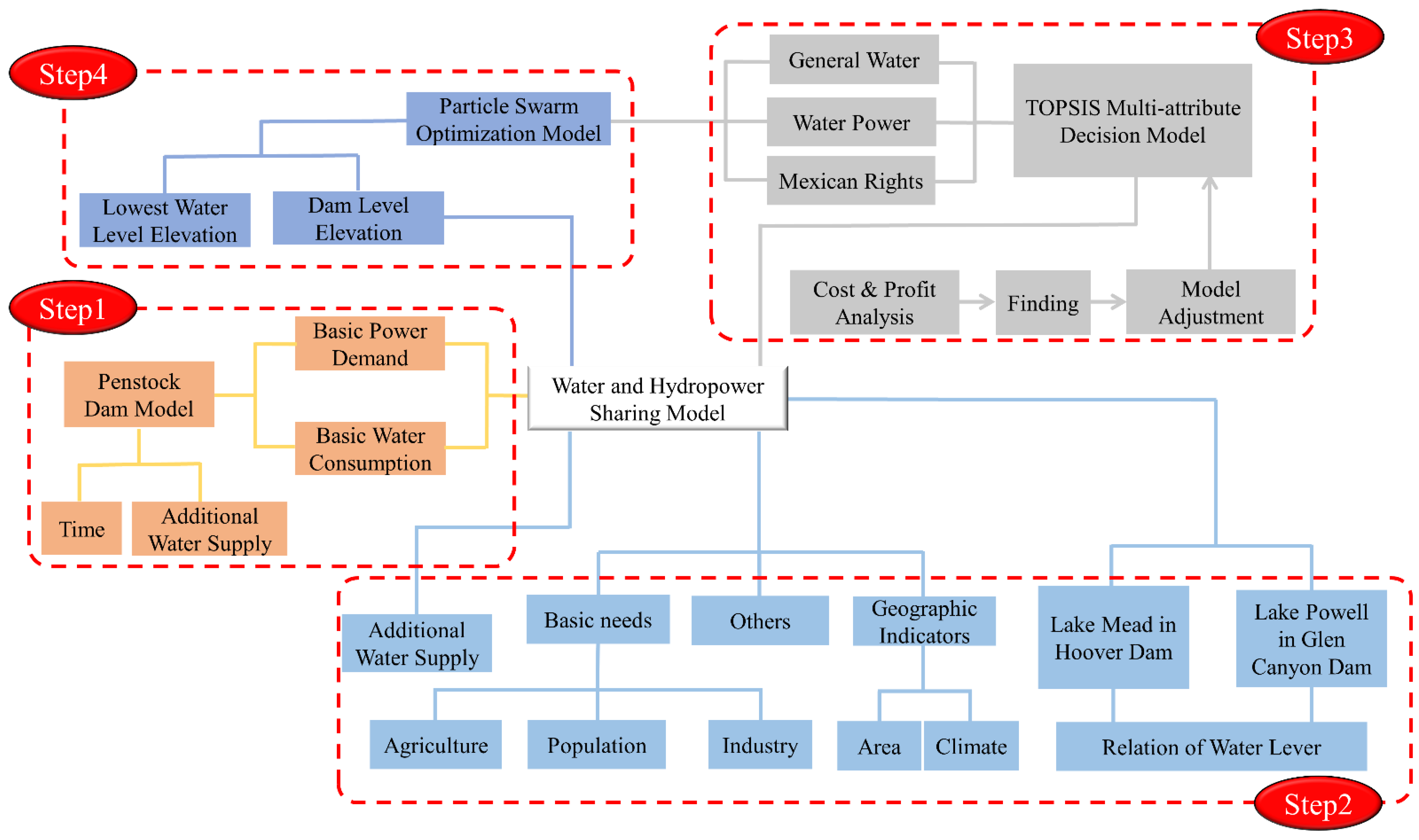
We would like to emphasize that the models we have developed are idealized mathematical models whose underlying sources are official data from various governmental organizations, and we believe that our work can have a positive impact on water resources management and sustainable development in the new context. Figure 1 roughly shows the framework of the work done. Briefly, this work considers the base power demand and water consumption in Step 1, and also accounts for the dam generation model, corresponding to the problem analysis in Section 2 and the model assumptions in Section 3.1. In Step 2, the hydropower and water allocation issues are considered mainly in terms of agricultural, demographic, industrial, and geographical factors, corresponding to Section 3. Step 3 focuses on proposing decision options for the multiple attributes previously proposed, with special attention to the interests of Mexico. Step 4 is based on the newly proposed novel particle swarm optimization (PSO) algorithm for solving the model, giving the minimum water level requirement, and also proposing a water allocation scheme for the CR, taking into account the historical and current situation.
2. Problem Analysis
2.1. Basic Electricity Demand in Five States
A significant portion of the power resource is hydropower resources, which in turn are influenced by the amount of water resources [37]. Therefore, electricity consumption in the five major states radiating from the Colorado River Basin below the GCD will be considered first. To find out the exact data on electricity consumption on each stated to make our model be as close as possible to the realities, we chose the U.S. Energy Information Administration which is a principal agency of the U.S. Federal Statistical System responsible for collecting, analyzing, and disseminating energy information. The regional population N and per capita electricity consumption of the five states of Arizona (AZ), California (CA), Wyoming (WY), New Mexico (NM), and Colorado (CO) [38] are organized in Table 1.
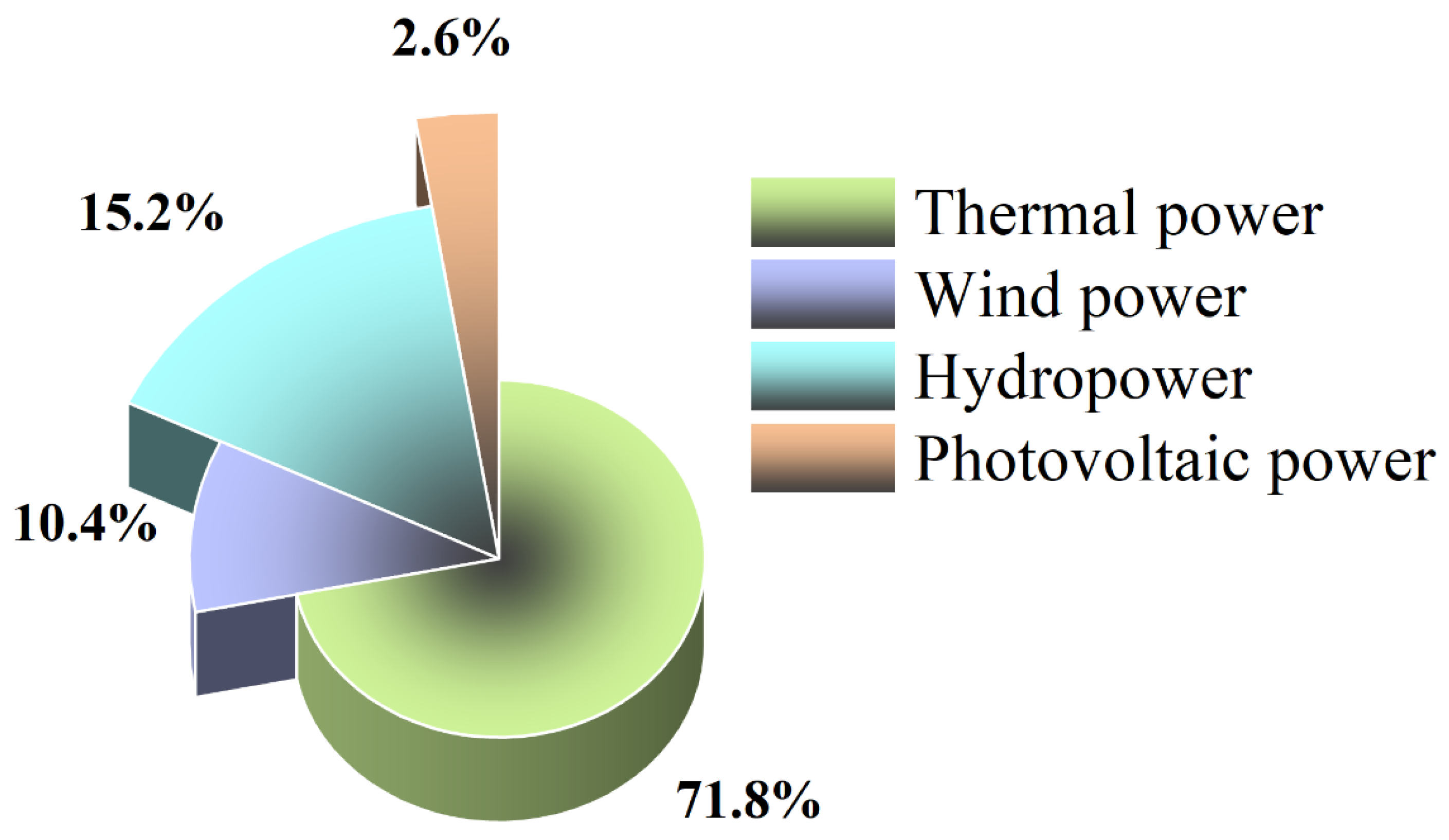
The proportion of hydropower in the total electricity generation of the five states in the region can be counted. The result is shown in Figure 2.
It can be directly obtained from Figure 2 that the proportion of basic hydropower generation is α = 15.2%. Thus, we can account the base hydropower demand in the region using the Equation (1):
where is represented as the basic electricity demand in kWh.
2.2. Basic Water Demand in Five States
To more rationally express the base water use, it will be idealized into three areas: residential water, agricultural water, and industrial water. Among them, the average water consumption of residences is represented as , while the average water consumption of agriculture is denoted as , representing the average water consumption per hectare of land, with the unit of . The average water consumption of industry represents the average water consumption per hour of operation of the plant, expressed as in . The number of inhabitants is denoted as , arable land area is denoted as , and the factory working time is denoted as in hours. Simultaneously, are used to indicate what proportion of residential, agricultural, and industrial water is provided by the CR basin. The final result of the base water consumption can be calculated using the formula below:
where represents the basic water consumption in tons.
3. Model Assumptions
3.1. Penstock Dam Model
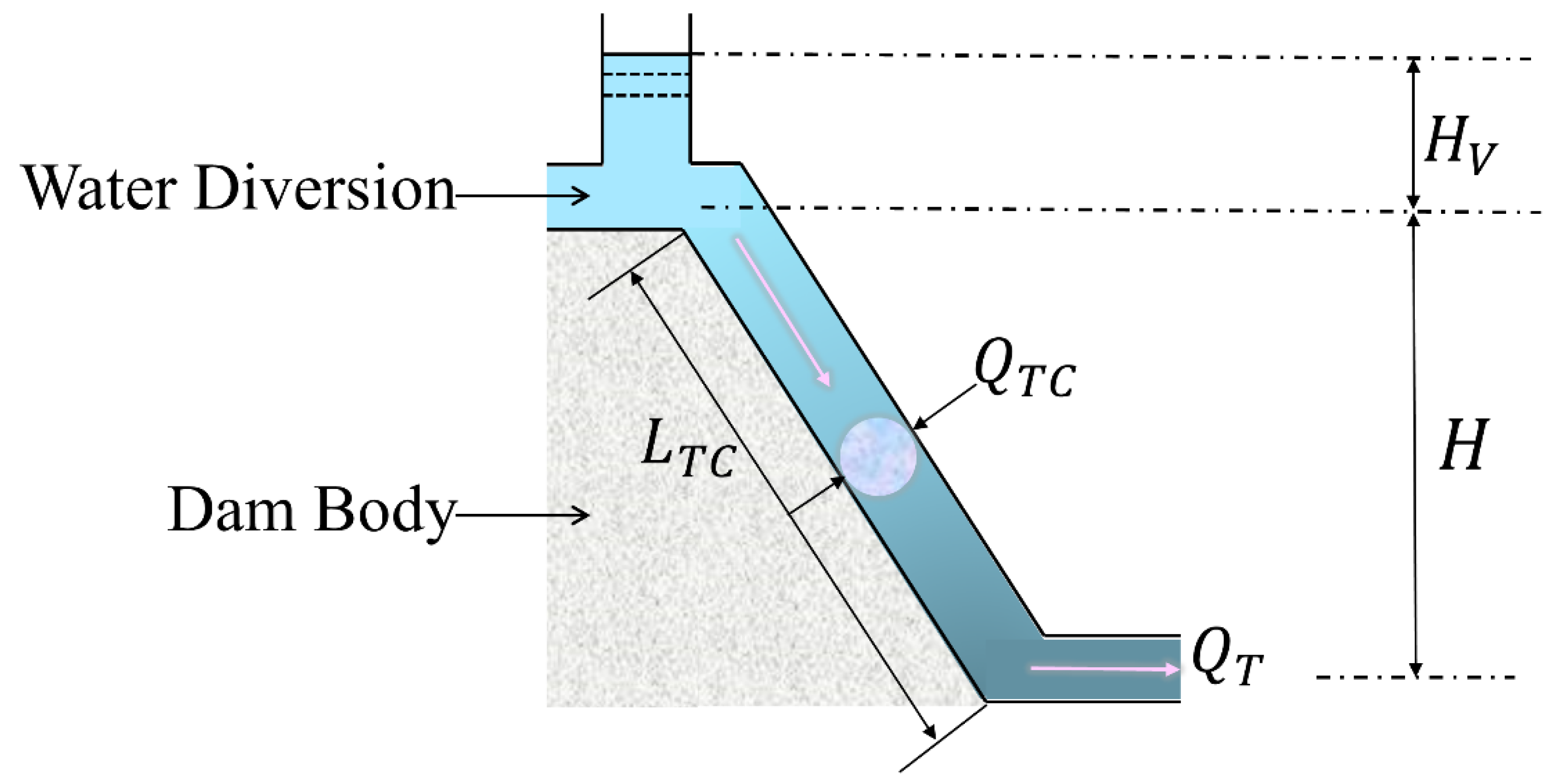
The structure of a hydropower plant is a complex issue, which is influenced by numerous factors, such as water level, water volume and efficiency of the generating unit [39]. The main purpose of this exercise is to rationalize the deployment of resources. It is imperative to find the answers intuitively and efficiently. Therefore, it is essential that the dam model be fully simplified. The simplified dam model is named the Penstock Dam model. Figure 3 shows a simplified schematic of it.
For the water flow of the pressure pipe, the following formula can be used:
where is the water flow of the Pressure Pipeline and H is the static head.
could be used to represent time constant, and it can be calculated by the following formula:
is the amount of water head loss, the calculation formula is as follows:
For , there is also the formula below:
where the parameter is calculated as:
At the same time, the formula for calculating the flow rate of water is:
where , the velocity of sound in water, is 1428 m/s.
The force of the water outflow is calculated as:
where N is the amount of electricity generated by the dam per unit of time, g is the acceleration of gravity, and is the generation factor of the dam.
The force of the water outflow is integrated into the time to obtain the power generation of the dam:
where represents the amount of electricity generated by the dam over a period of time.
3.2. Hydropower Allocation Model
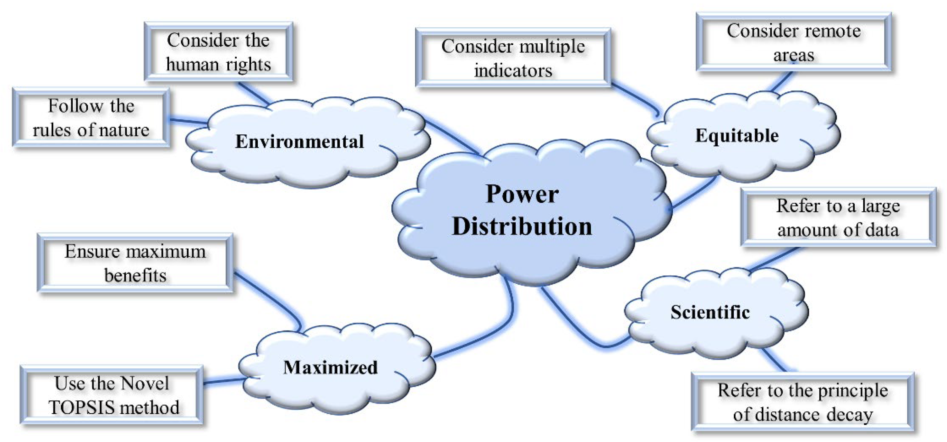
Electricity resources are the lifeblood of the national economy, and it is our unavoidable responsibility to reasonably allocate electricity resources and fully meet the people’s demand for electricity resources. In allocating the power resources of the Hydropower Station, we took the principle of Environment, Equity, Science, and Maximization into account, fully considered the power demand of each industry in each region and the actual geographic situation, selected the multi-attribute decision analysis method in system engineering for the finite scheme, comprehensively analyzed the power demand of 173 counties in five states, and appropriately simplified the model. The specific distribution concept is presented in Figure 4. We constructed the improved Technique for Order Preference by Similarity to an Ideal Solution (TOPSIS) method based on four major attributes using limited data, to provide scientific guidance for power resource allocation.
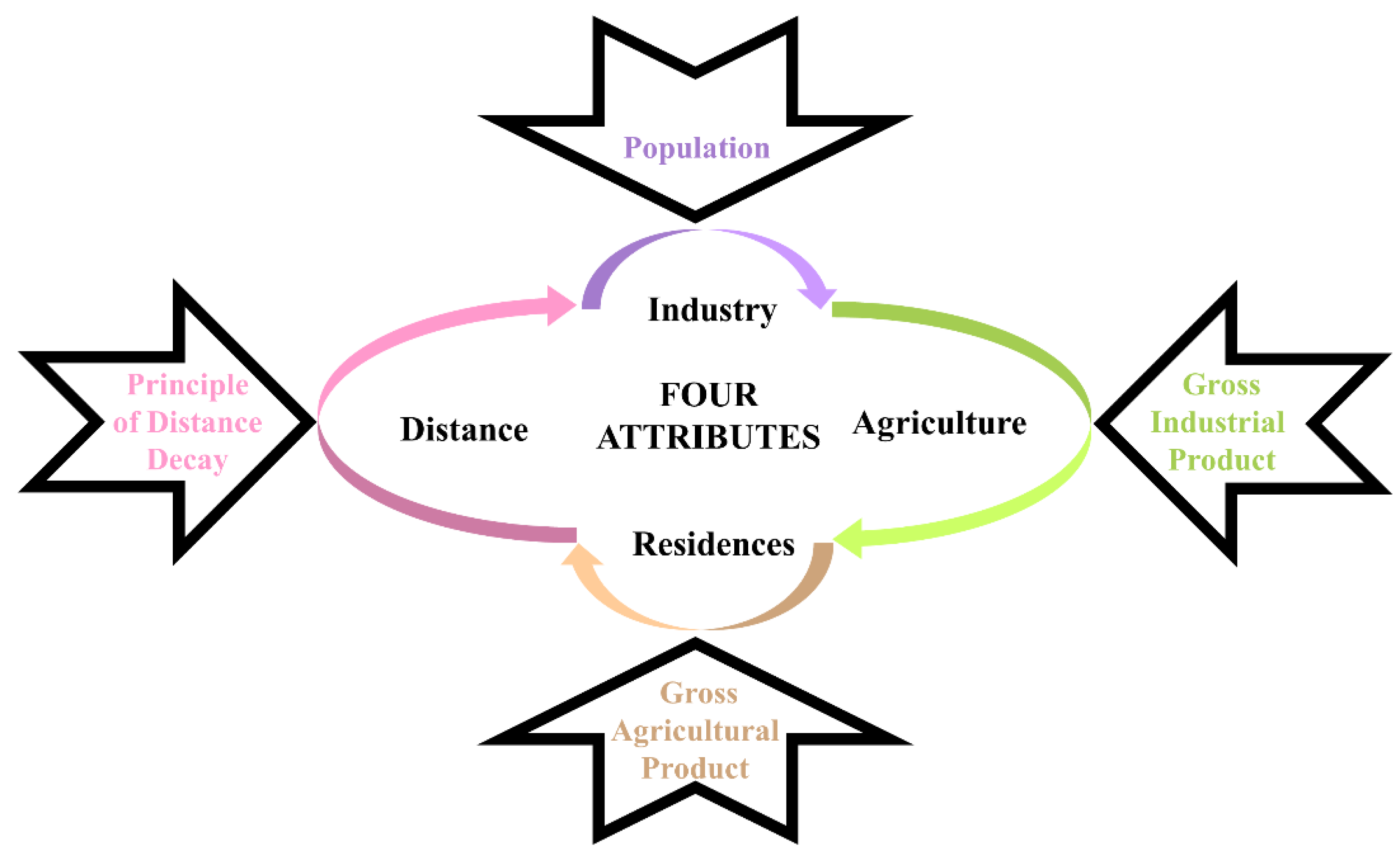
It is well known that among the five states given in the problem, the Economic Level, Population Size, Geographical Location, and Industrial Structure vary greatly from region to region. Adequately quantifying the attributes and collating the indicators is a difficult task. Politicians believe that the economic foundation determines the super structure. In selecting the indicators, we took the three major types of electricity consumption (agriculture, industry, and residences) as the grasp to organize the 193 counties in 2020 corresponding to agriculture production, industrial production, and population changes from the United States government official online website, which contains the most specific information relating to our model [40]. They are an important medium to quantify the attributes. Figure 5 shows the correspondence between attributes and indicators.
When considering the geographic location factor, we introduce the Distance Decay Law (DDL). The essence of the DDL is that the interaction between geographic elements is related to distance, and the interaction between geographic elements is inversely proportional to the square of distance when other conditions are the same [41]. The theoretical basis of the DDL is the formula of universal gravitation discovered by Newton.
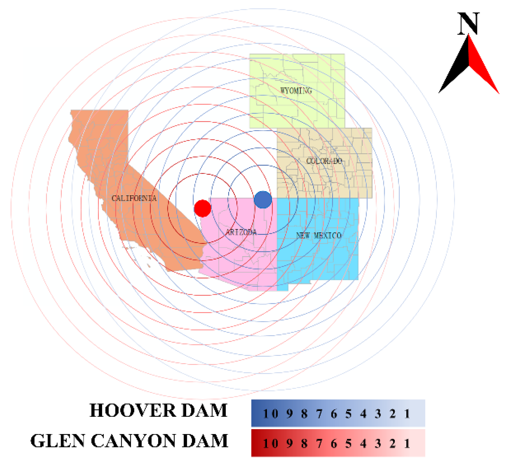
We counted the distance from 193 counties to the two dams, and also combined the power resource allocation principles to quantify the distance index and transformed the distance merit into 10 levels from 1 to 10 points. Figure 6 graphically illustrates this work.
Population, Gross Agricultural Product, Gross Industrial Product, population, and distance distribution values to GCD and HD were statistically compiled for the 193 counties in the four states in 2020. Table 2 shows the results for the selected areas.
The TOPSIS method is a common decision-making technique for multi-objective decision analysis of finite solutions in systems engineering [42]. In recent years, it has also been used in the comprehensive evaluation of multiple indicators. In our problem, we need to consider the power resource allocation of 193 counties in five states, but we cannot accurately consider the importance of the four indicators, and the traditional TOPSIS method needs to determine the attribute weights in advance, which is more subjective [43]. Based on this background and demand, we propose a model of power resource allocation based on the Novel TOPSIS method.
Firstly, m evaluation indicators are selected for n evaluation units for comprehensive evaluation (forwarding of inverse and moderate indicators), and the original data matrix X is as follows:
Then, the data are normalized as:
Here, Z is represented as the unit matrix obtained after the normalization of matrix X. i and j represent only the corresponding element positions in the matrix. k represents the term k in the summation. i, j and k have no special meaning. Where:
The optimal value and the worst value of each index can constitute the optimal value vector and the worst value vector :
The distances of each evaluation unit from the optimal and inferior values can be calculated, respectively:
The relative proximity of each evaluation unit to the optimal value can also be calculated:
The traditional method ranks the relative proximity, and the larger the relative proximity, the closer the evaluation unit i is to the optimal level.
- Determining the weights
The highlight of this work is the improvement on the traditional method. The first step of the improvement work is to build an extended multi-attribute decision matrix based on the matrix Z:
where , corresponding to m alternatives, , corresponding to , and the weights of the attributes S can be reflected as:
The corresponding weighted normative matrix is calculated as:
From Equation (19), we can see that the smaller the is, the larger the is. To further determine the indicator weights, the objective planning optimization model is constructed as follows.
It can be defined that:
Let the Lawrencian function be:
Assuming that:
Thus, we can obtain:
and it is solved as:
There is and is a minimum value point of the objective function of the optimization model.
- Improving positive and negative ideal solutions and relative proximity
In the normalized decision matrix R, satisfies . The value of the objective attribute corresponding to the highest preference is , and the value of the objective attribute corresponding to the lowest preference is , so that . Moreover, the negative ideal solution is (where ).
From this, it is deduced that:
The improved relative proximity is obtained as:
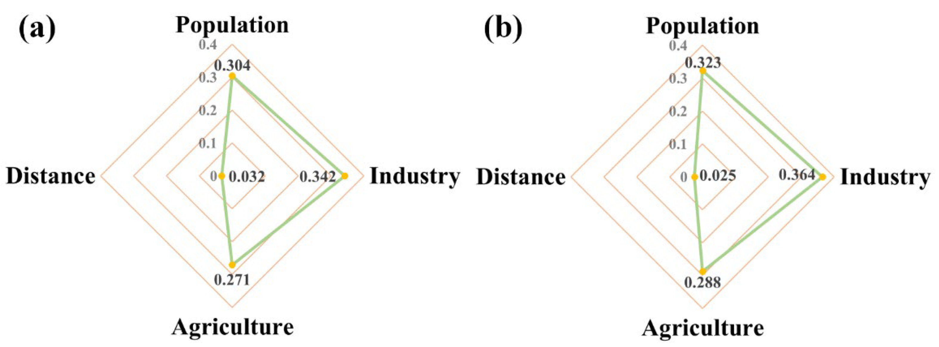
Each of the four attributes is assigned to a weight in this model. Figure 7 reflects the results obtained from the calculation. From the weight distribution, the power distribution is mainly influenced by the three attributes of agriculture, industry, and residences. Moreover, these three attributes have a similar impact, while the geographical location has a relatively small impact on it. In practical terms, the power resources generated by hydroelectric power plants will be injected into the well-connected power network, and the disadvantages caused by distance (such as loss, time, and other factors) can be almost negligible in front of the three demands of agriculture, industry, and residences. However, when the three demands of agriculture, industry, and residences are almost similar, distance will have a strong impact on our distribution scheme. The weight distribution fully demonstrates the rationality and scientific validity of our improved model.
Figure 7.
The weight distribution of four major attributes. (a) The HD. (b) The GCD. The relative proximity of the 193 counties to HD and GCD was calculated using the improved model derivation. The results are presented in Table 3.
Figure 7.
The weight distribution of four major attributes. (a) The HD. (b) The GCD. The relative proximity of the 193 counties to HD and GCD was calculated using the improved model derivation. The results are presented in Table 3.

3.3. Water Allocation Model
From the water statistics from government’s official website [44] and visualized images (Figure 8), some water from GCD will be provided to LP. This fact further illustrates the important relationship between the two waters, which is that LP can be considered a sub-water of LM. From an idealized perspective, the higher elevations would be supplied by LM, not LP. The water supplied from LM, to lower elevations (e.g., CA), can be considered as part of its supply to Powell. When the water level of LM is M and the water level of LP is P, to draw water from each lake, the demand models of the five states are referenced to fully consider the water supply requirements of both lakes. At the same time, by the upstream location of LM in dry LP, the two lakes are fully connected and continuously deliver water resources, so the following cases are analyzed to improve our model.
When P > Pmin, M > Mmin, the water levels of the two lakes meet the power generation requirements of the two dams at this time. In reality, the water resources allocation model is related to the water delivery link, i.e., the distance of the two lakes to each state. Thus, it is necessary to consider water allocation in terms of geography to find the optimal solution.
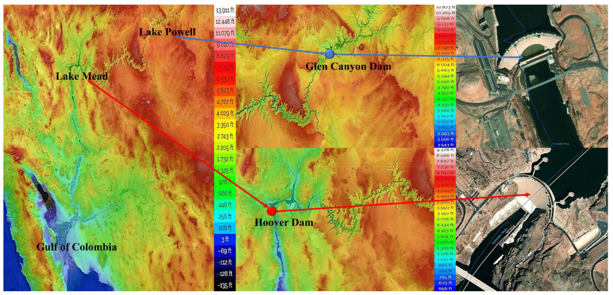
We can visualize through the satellite map that part of the CR connects the two waters. As can be seen in Figure 9, the water flowing from LP to LM will be in a canyon with an elevation of 4000–5000 ft.
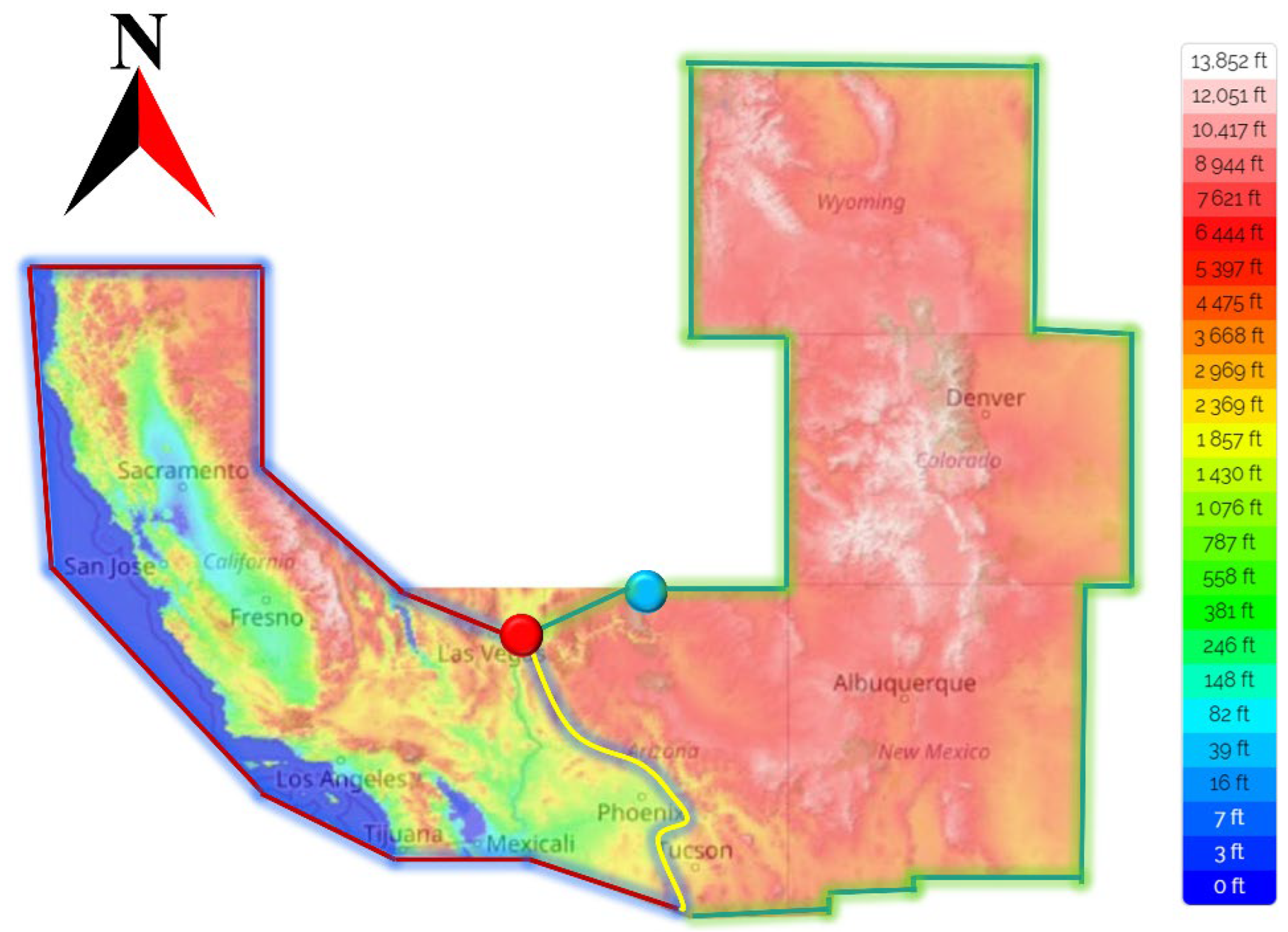
ArcGIS software shows that the average elevation of the area to the left of the yellow line in Figure 10 would be less than 1000 ft and that the water flowing from LP could theoretically be used in the area to the left of the yellow line. To the northwest of LP, the higher elevation of Death Valley National Park, an important reservoir in north-eastern CA, would allow some of the water from LP to flow there. Again, looking at the entire geomorphic map, in our model, LP would theoretically provide water for the entire CA region. Therefore, we have assigned LP the water supply area within the red boxed line in Figure 10. For LM, since it is theoretically difficult for water from LP to flow to higher elevations 11/21 within the five states we set, the water supply task for higher elevations is given to LM, i.e., the green boxed part in Figure 10.
3.4. Other Cases
- When the water level of LM is higher:
The water supply of LM should be used preferentially. For the geographic water supply model, it is important to compare the scores that each state gets for distance by assuming that each state applies a single water supply model and improves the criteria for the allocation model to decide on the water supply of a particular lake based on the scores. In other words, if the difference between the distance weighted scores of two lakes to a state exceeds 30, the single lake water is considered to be extracted to provide water for a state, and if it is less than 30, the lake water is extracted to provide water for a state proportionally.
- When the water level of LP is higher:
When LP is upstream of LM, it is going to be necessary to compare the five-state water supply geographic scores of the two lakes, while it is important to further consider the water release capacity of GCD. It is assumed that with benefit as the priority decision goal, the upper reaches of the river can flow downstream by gravitational potential energy, which is a process that requires far less cost than the transportation cost of drawing water from the lake. Based on this consideration, the benefit scoring part of the model is used to evaluate the benefit and geographic factors together. This results in the proportion of flow from LP to LM, and thus, the water supply model for both lakes.
4. Establishing and Solving the Model
4.1. A Study of Data from the HD and GCD
The average annual elevation of the HD can be calculated from 1963 to 2022 and the change in water capacity can be visualized by plotting scatters. The result is nonlinearly fitted through MATLAB software with a confidence interval of 95%, and the fitting equation is as follows:
The R-square of this fitted model is 0.8994. Thus, we believe that this model has an extremely high predictive value for the HD water level between 2020 and 2040. The fitted curve is shown in Figure 11a. Under the same conditions and through the same means of operation, the average annual altitude of the GCD from 1963 to 2022 and its nonlinear fitting map could be obtained. The fitted equation is as follows:
The R-square of this fitted model is 0.9677. Thus, we also believe that this model has an extremely high predictive value for the GCD water level between 2020 and 2040. The fitted curve is shown in Figure 11b.
4.2. Length of Time That Can Meet Demand
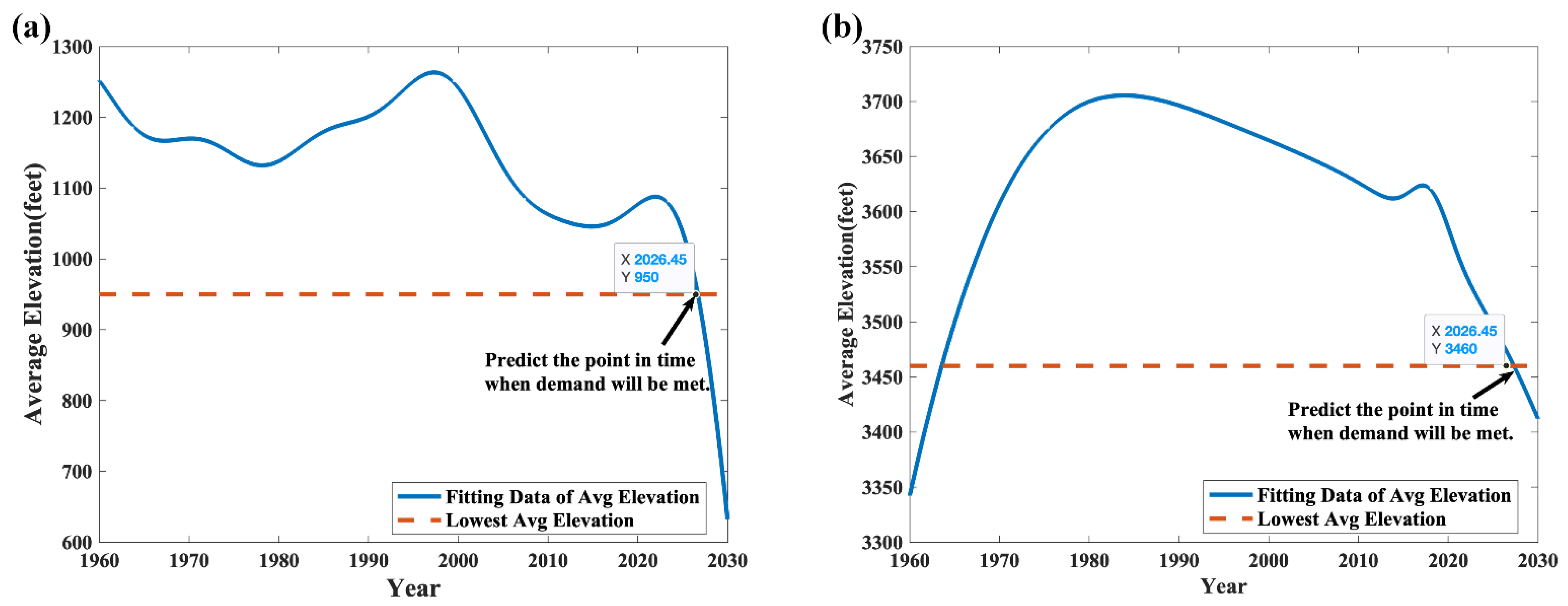
The statistics of basic water consumption and basic electricity consumption are substituted into the model on the basis of the hydroelectric power generation model. The minimum water level heights of the two dams were calculated as: 950 feet for the HD and 3490 feet for the GCD. The minimum water elevation represents the critical data that can meet the normal water and electricity needs of the people. It is a very scientific method, using the fitted equation in the ideal state. Figure 12 visualizes the water level elevation of HD and GCD in the future period. If the dry heat persists and people do not take relevant measures, HD will not be able to generate enough electricity to meet the basic needs of the nearby residences by June 2026, and GCD will not be able to meet the basic needs of the nearby residences by May 2027. Therefore, if people do not make timely adjustments, the residences of the area will face the dilemma of not being able to meet their basic electricity demand in about 5 years under the continuous influence of drought and hot weather.
4.3. Demand for Additional Water
There are a series of measures to be used to meet the basic needs of the population for a longer period in today’s harsh environment. Introducing additional water into HD and GCD is a very straightforward solution to this problem. Then, we will have to determine the minimum amount of water that needs to be brought in to meet basic needs.
First, obtain the value at which the dam water level falls below the minimum water elevation after the base power demand cannot be met:
where is represented as the altitude below the lowest water level at t time in m. Then, through the Formula (35):
where V is represented as the Volume of water that needs to be introduced or be available in .
We can calculate the volume of water that needs to be introduced to each dam at time t. The results in Figure 13 show that the HD will need to introduce additional water in the second half of 2026. The amount of water to be diverted will increase over time. If sufficient water is not brought in promptly, the basic needs of the residences in the area will not be fully met and daily life will be affected.
GCD is located at the headwaters of the river and has an abundance of water, so it can meet the daily needs of residences for a longer period in a dry, hot environment. However, according to the Simulation Forecast in Figure 13, it will be unable to meet the daily needs of residences by 2027. However, GCD requires significantly less water than HD, and GCD will also maintain a steady increase in the amount of water introduced into the dam. According to the results of the model, tons of water should be introduced in 2018, and in 2029, there should be tons of water. The data are a constant reminder of the need to act as soon as possible to actively and effectively prevent or delay this situation, using the available scientific and technological means.
4.4. The Solution of Water and Hydroelectric Competing Interests
Under the condition that the basic water requirements and basic electricity requirements of the five states are guaranteed, selecting maximum profit as the criteria when resolving conflicts between water for general use and water for power generation. The excess water resources will be allocated reasonably to maximize profits.
First, obtain the average water level elevation of GCD and HD to get of allocable water resources for each of the two dams. Then, we ought to consider the general water use (residential, agricultural, industrial), power generation, and Mexican water entitlement at the same time, so the water allocation plan maximizes the interests of the five states while ensuring the rights and interests of Mexico can be obtained.
Let the general water allocation of GCD be and the power generation water allocation be . HD has a general water allocation of and a power generation allocation of . The final flow to Mexico is .
4.4.1. Calculation of the Net Profit of General Water Use
Divide the general water use into residential, agricultural, and industrial water use. Assuming that the proportion of residential, agricultural, and industrial water in general water use is , , , respectively, and that the treatment costs for different uses are , , , respectively, the treatment costs for general water use can be expressed as:
Here, i represents the term i in the summation and has no special meaning. For all counties in the five major states, the transportation cost coefficients are classified as based on the distance from the dam. Additionally, based on the water allocation model we developed earlier, the transportation cost can be obtained as:
By querying the water rates in different areas, we can derive the total revenue that can be created by these water resources as:
This leads to the net benefits that can be obtained from general water use as:
4.4.2. Calculation of the Net Profit of Water for Power Generation
First of all, according to the amount of water allocated for power generation, we can get the amount of power that can be generated by the two dams as and by substituting it into our dam power generation model. Second, let the cost of producing one degree of electricity at GCD and HD be and , respectively, so the cost of power generation is:
Similar to the transportation cost of water in general, the transmission cost coefficient is divided into and the transportation cost is:
Combined with the specific electricity prices in different regions, the total return can be obtained as:
Thus, the total profit can be obtained as:
4.4.3. Guarantees for Mexican Rights and Interests
The establishment of HD stopped the flooding of the CR and allowed the water resources to be fully utilized. The CR was able to water more U.S. land. Later, the U.S. built 14 reservoirs and 32 large irrigation projects on the CR. In a way, the CR is in the hands of the United States and is the best-regulated river in the world in terms of water resources. However, because of the endless demand for river water by cities and agriculture along the CR, there is a serious water crisis here. The uncontrolled use of water resources has also resulted in a huge waste of water resources. Because of the uncontrolled claiming of river water by the United States, Mexico has lost its most fertile agricultural area, which is a serious violation of Mexican rights. Based on relevant information, we believe that Mexico has sovereignty over the water resources left after the five states have consumed their share. Therefore, we compare the agricultural land, population, and industrial power of Mexico and the United States in the CR Basin to determine the Mexican share of the CR Basin. The data show that the CR Basin supports about 40 million people, of which five U.S. states, AZ, CA, WY, NM, and CO, account for about 35 million. Meanwhile, the farmland affected by the CR in five U.S. states is about 1 million hectares, and the farmland affected in Mexico is about 400,000 hectares [45]. Considering the industrial level and scale of the five U.S. states and Mexico, as well as the long-term average natural flow of the CR, the following scenarios are derived. (1) When the annual natural flow of the CR is above or below the long-term average natural flow (12.4 million AF), the U.S. would need to import 1.5 million AF of water into the Gulf of CA. (2) When there is a drought and the annual natural flow of the CR is much less than the average natural flow, the U.S. can import 12% of the annual natural flow into the Gulf of CA, depending on the natural flow of the year. (3) When the annual natural flow of the CR is much greater than the average natural flow, the United States needs to import 14% of the annual natural flow of water to the Gulf of CA.
At the same time, if the United States does not import enough water to the Gulf of CA, the United States will compensate Mexico according to a certain scheme to maintain Mexican rights and interests. Assume that the normal price of water for the year is p. Table 4 shows the compensation plan for Mexico and the corresponding program design.
Combining the above equations and compensating for the Mexican program yields. The objective function is:
The constraint conditions are:
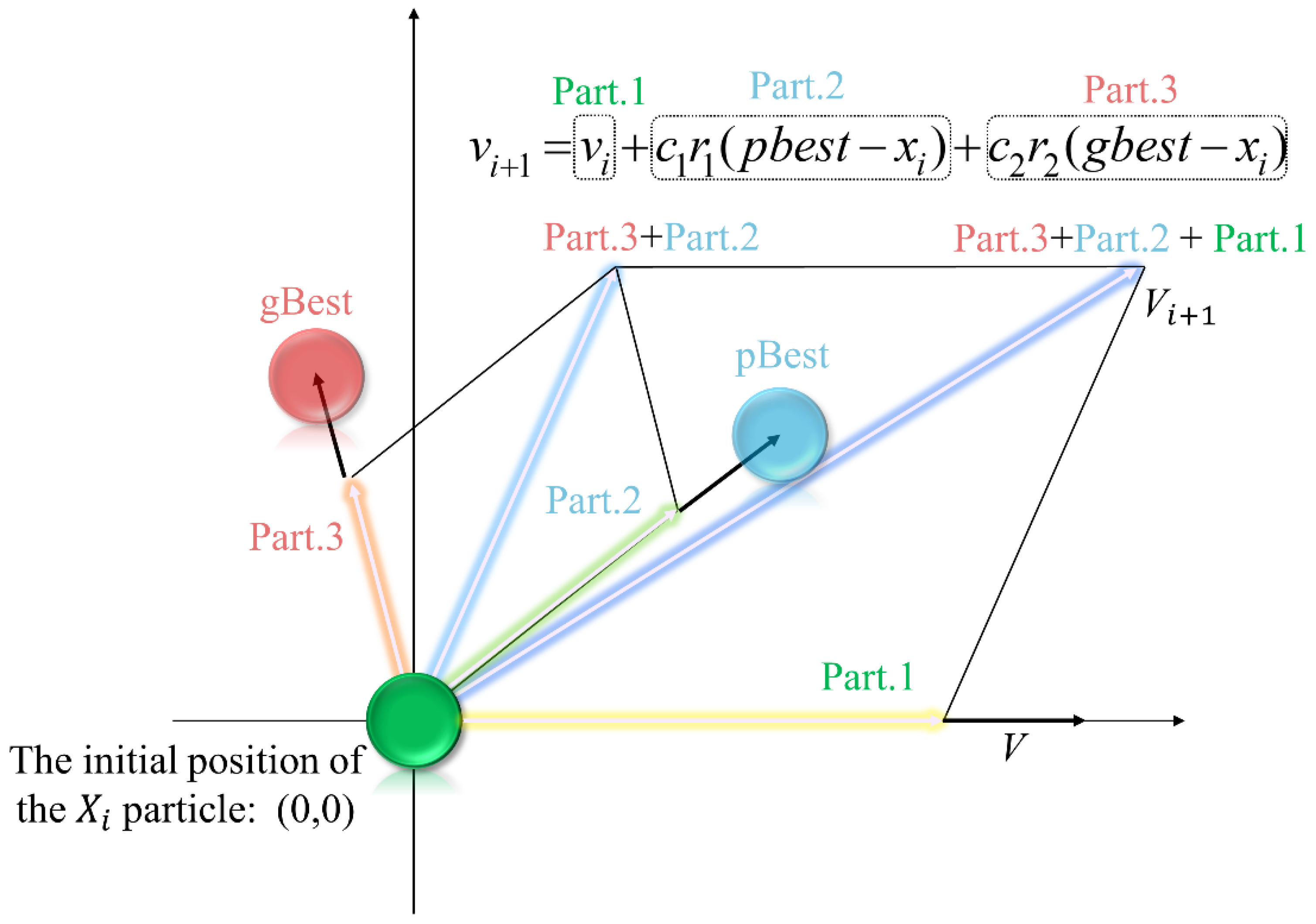
The location path formulation of the standard Particle Swarm Optimization (PSO) algorithm always fluctuates in a fixed interval and is prone to fall into the situation of locally optimal solutions [46]. To solve this problem effectively, we improved the PSO algorithm. The oscillating convergence function is added to the algorithm to make it jump out of the local optimal solution and improve the search performance and accuracy of the PSO algorithm [47]. Figure 14 graphically illustrates the processing. The evolution equation of this PSO is:
where is the velocity of the particle i in iteration k, is the velocity of the particle i in iteration k − 1, which is known as the first part, is the cognitive constant, is the maximum fitness of the particle i in iteration k, is the position information, is known as the second part, is the Random function, is the maximum value of all pbests, and is known as the third part.
The position update function is:
The loop is terminated when the maximum number of iterations is reached or the acceptable satisfactory solution is within a specified range.
The evolutionary velocity and position equations for the traditional method [47] of introducing second-order oscillatory links are:
Oscillatory convergence of the algorithm: ; asymptotic convergence of the algorithm: .
The improved particle velocity equation and position equation are Equation (51) and Equation (52), respectively.
We calculate and simplify this equation by derivation to obtain the constraint of :
where is a random number with restricted values, also known as the oscillation parameter.
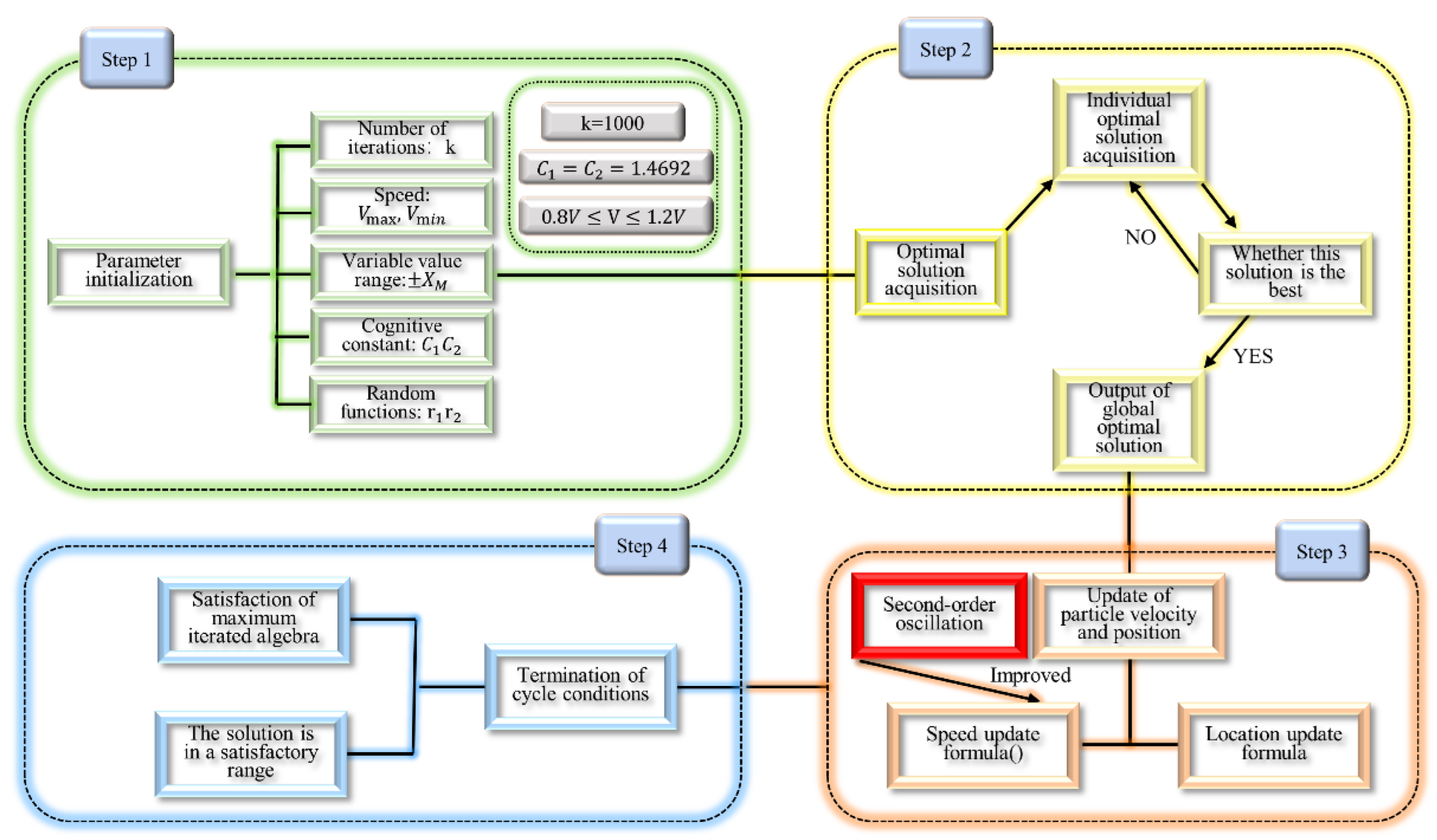
This work improves the oscillation parameter of the second-order oscillatory PSO algorithm and determine its more accurate range of values, so that the algorithm converges oscillatively in the early stage and converges asymptotically in the later stage, increasing the global convergence capability of the algorithm and improving the convergence accuracy of the algorithm. The whole thinking process is reflected in Figure 15. We conclude that the maximum benefit to the five states can be achieved at 38.6% for general water use and 47.5% for power generation.
4.5. Analysis of Results
4.5.1. Growth of the Population, Agriculture, and Industry in the Affected Area
When the population, agriculture, and industry in the affected area grow, the population, agriculture, and industry in the area grow accordingly. That also means an increase in base water use and base electricity use. Substituting the increased basic water use and electricity use into the dam power generation model will result in a corresponding increase in the minimum water level. This indicates that the time required to meet the basic needs of the population will decrease, holding other factors such as climate and rainfall constant.
4.5.2. Improving the Use of Renewable Energy Techniques
Improving renewable energy techniques means an increase in the use of renewable energy technologies, such as hydroelectric power and wind power, which also means that we can use as much water as possible in dams to generate electricity. This will lead to an increase in the amount of electricity generated by dams, which will be used more by the population.
4.5.3. More Water and Electricity Conservation Measures Are Implemented
More water and electricity conservation measures will lead to a reduction in basic water use and basic electricity use. Substituting the increased basic water and electricity use into the dam power generation model will result in a corresponding reduction in minimum water levels. This will leave more water at our disposal. Our modified PSO algorithm can be used to obtain optimal water allocations for general use (residential, agricultural, and industrial) and power generation, thus maximizing our returns. It will also better guarantee the rights of Mexico.
4.6. Coping with Water Scarcity
From the model, we can see that when water resources are not enough to meet all the hydroelectricity demand, it is easy to think that “broadening revenue sources and reducing costs” is an effective way to solve the problem.
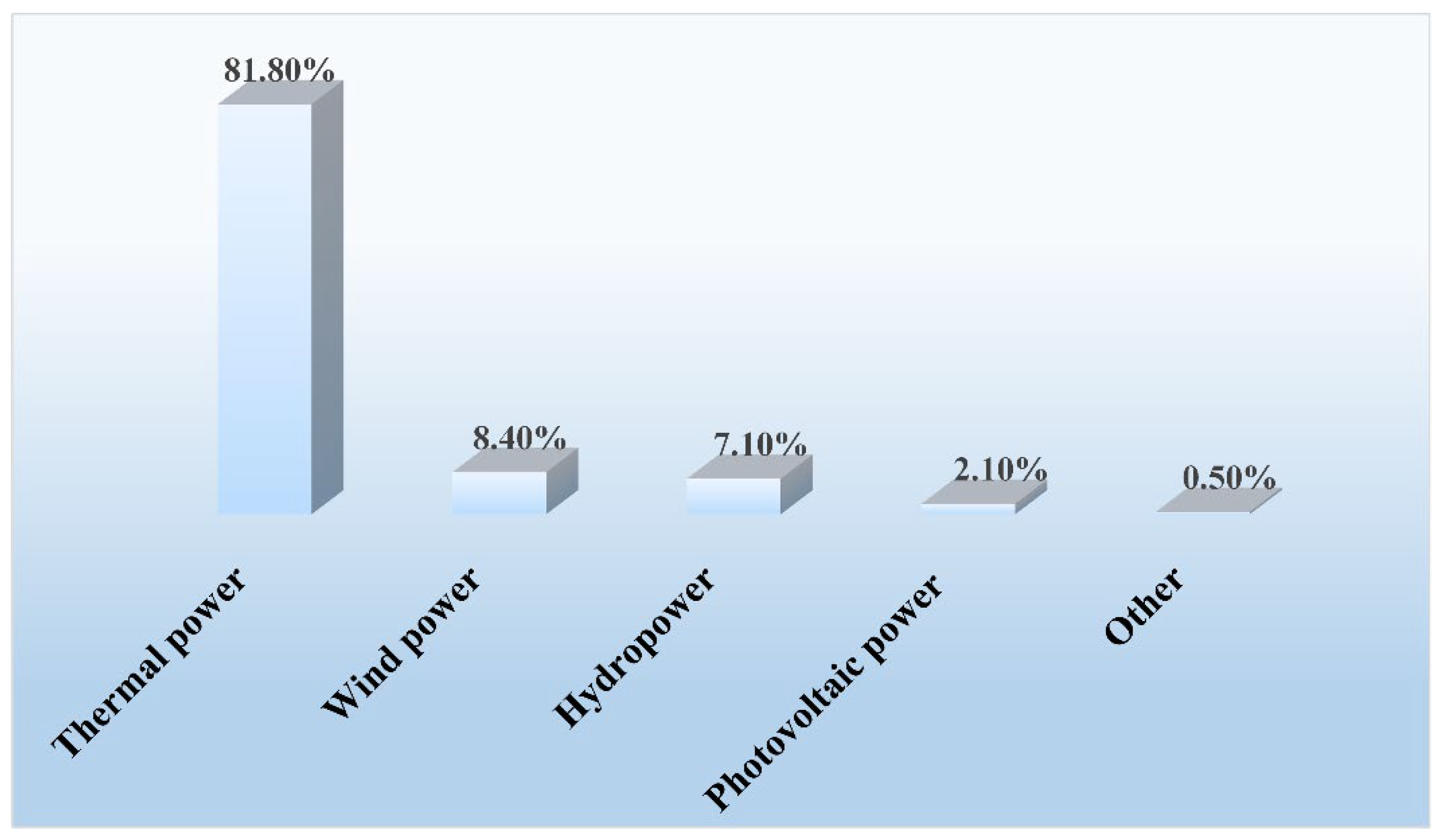
“Broadening revenue sources” means seeking new renewable energy sources to produce electricity so that the total generation capacity rises to meet the basic electricity demand as much as possible. We obtained data from EIA [48] that the United States is still dominated by thermal power generation, which accounts for 81.80%. Hydropower generation accounts for only 7.10%. Figure 16 presents the specific proportions. Therefore, it can be supplemented by strengthening other power generation methods to meet the basic electricity demand. In terms of water resources, research related to seawater desalination and other research can be increased, and if there is a breakthrough, the source of freshwater can be greatly improved, thus solving the water problem.
“Cost reduction” means strengthening water use management through administrative, technical, and economic management means, adjusting the water use structure, improving water use methods, and using water in a scientific, rational, planned, and focused manner to improve the utilization rate of water resources and avoid waste. At the same time, the state should put forward corresponding policies to make the concept of conservation deeply rooted in people’s hearts to reduce the basic water and electricity demand in people’s life and production.
5. Evaluation and Improvement of Model
Firstly, the priority of several models innovatively proposed in the work is fully discussed and the important role played by each of them is argued. The PD model is based on the actual power plant situation and the two-sided consideration of model prediction accuracy, cleverly ignoring factors unrelated to the power generation of the hydropower plant and capturing the core elements such as water level height and water flow. Compared with other models of the same type, the PD model has the advantages of easy implementation and high accuracy.
The TOPSIS method is a common decision-making technique for multi-objective decision analysis with finite solution in system engineering. It has a wide application in the comprehensive evaluation of multiple indicators. Considering the importance of the relevant indicators that cannot be accurately obtained for our problem, we have improved the traditional TOPSIS method. The Novel TOPSIS method can determine the weights of relevant indicators more objectively and make the model more accurate compared with the traditional TOPSIS method.
Water resource allocation mainly requires consideration of water transmission distance and transportation cost. Therefore, we consider water resources allocation from a geographical point of view, visualize each area by satellite map to divide it and obtain the water transmission score, and then obtain the water transmission scheme according to the score.
The PD model can obtain the predicted values of dam power generation and total water availability more accurately and easily. The Novel TOPSIS decision model can help us to optimize the allocation of power and water resources according to the relevant requirements. Ultimately, the water allocation model can be used to rationalize the allocation according to distance and transmission costs.
In the previous discussion of the main water and hydropower resources and the balance between them, the essence cannot be separated from the healthy operation of the dam. That is, the adequate deployment of upstream and downstream water resources to meet the water demand of each region and the required water flow for power generation. Therefore, we believe that it is necessary to discuss the previously established PD model to explore its scope of application, so as to further improve this work. From Equation (9), it is easy to see that the power generation of the dam per unit time in the idealized model is proportional to the average water level elevation of the dam.
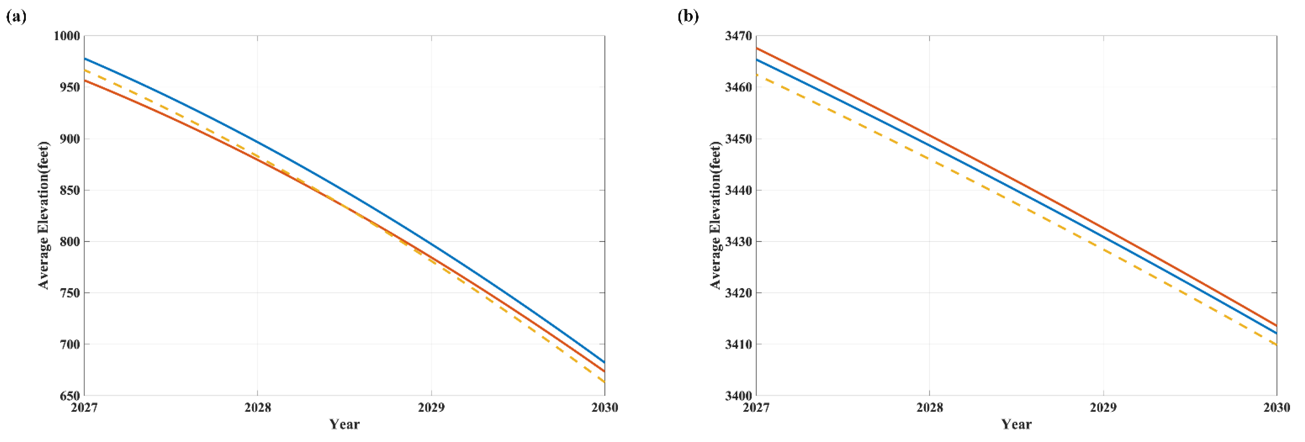
Therefore, to perform a sensitivity analysis of the effect of the mean water elevation on the model results, we have to make a small fluctuation up and down in the mean water elevation, and the effect on the predicting results of the dam water level prediction model is shown in Figure 17.
It can be seen that when the average water elevation fluctuates slightly up and down by 1%, the predicting values for HD also produce corresponding small changes, i.e., a 0.91% increase and 2.36% decrease. The corresponding increase and decrease for GCD are 1.23% and 1.57%. The results prove that the dam water level prediction model has good sensitivity and can meet our daily needs better. Using a similar approach above, we performed a sensitivity analysis on the dam power generation model as well, where there is a corresponding 5.23% increase in power generation when the input water level height of the dam power generation model changed by 5%. This result is in line with our expectations, while also meeting the needs of our TOPSIS allocation model and PSO algorithm.
In general, models based on idealized assumptions are important for guiding actual water and hydropower resource allocation. However, it has to be admitted that there is a gap between the ideal and the reality. Therefore, this paper also prospectively suggests some points that should be focused on in a realistic analysis, especially assumptions that have a significant impact on the analysis. We believe that this will further enhance the practical value of this work.
First, the dam power generation model presented in this work when studying the allocation is simplified, and the text cleverly considers two dams, in a sense unifying the properties of the two dams, which we consider an interesting means of treatment. However, it must be stated that for different dams and power generation models, a case-by-case analysis should be made to ensure the scientific and accurate nature of the model.
The consideration of geographic factors in the allocation process is also worthy of further research. This work quantifies the complex geographical factors simply in order to simplify the mathematical model. However, in future studies, full consideration of altitude [49], climate [50,51], biology [52], and other factors is considered necessary.
A direct division of water resources based on a single elevation relationship is not necessarily applicable in all cases. Further studies should specifically consider the relationship between the two reservoirs and the differences in water use by region, and the important role played by groundwater [52] and geological conditions [53] should also be considered.
It is important to emphasize that the simplification of assumptions necessary for this paper to consider multiple factors in a holistic manner proves to be valid. Its mathematical modeling perspective presents the complex analysis in a simple and wonderful mathematical language that guides the issues of power generation from the two dams, the allocation of water and hydropower resources in the five states, and the resource entitlements involved in each location.
This work compiles and analyzes the history, present, and future of the CR from a large body of data in which the water and hydropower resources of the southwestern United States and Mexico were fully deployed. Despite the many unique features and developments of the ideas and work, it has to be admitted that they have many limitations. First, the accuracy of the model is still open to question due to the over-reliance on official datasets. Second, some of the work performed is too idealistic, and many of the means of treatment are based on assumptions that do not have a distinct realistic extension value. Third, the mathematical methods used in the targeted research questions selected are not always accurate. Fourth, the model still has limitations. This is mainly due to the fact that the model assumptions we have developed are all built in this particular geographical location and spatio-temporal environment, and their generalizability is not obvious. The future developments are still needed to introduce other important influencing factors, such as climatic conditions and bio-diversity, and modularize the problem with a more scientific model from both the perspective of reference data and practical investigation, and then integrate a complete and scientific planning system to contribute to the sustainable development of the watershed represented by CR.
6. Conclusions
The CR water crisis needs to be solved urgently. Based on official datasets and at-lases, we proposed and optimized models for dam power generation, water resource allocation, and hydropower resource allocation, taking into account agricultural, demographic, and geographic factors, designed a decision scheme using the TOPSIS method, and conducted a PSO algorithm to find the optimal means of solution. We tested the model and the algorithm with actual data model at this stage and got scientifical prediction about the minimum water elevation requirements for LM and LP would be 950 ft and 3460 ft, respectively. It can warn the authorities of the need to take measures and be of help when making solutions to avoid the days in 2026 or 2027, when, according to our analysis, LM and LP are not able to meet the water and hydropower demands, respectively. Specific feasibility options for the measures were presented, including diversions and proportional allocations, and also took into account the rights and interests of Mexico. Compared to previous studies, this work is comprehensive and forward-looking, with a mathematical construction method that takes into account multiple complex factors and a decision scenario that integrates history and current status expected to be an effective follow in the field. Meanwhile, comprehensive and scientific models incorporating climatic, biological, geographic, and economic factors are expected to be proposed in further studies.
Author Contributions
Conceptualization, Q.Z. and H.H.; methodology, Q.Z. and M.F.; software, J.H.; validation, Q.Z., H.H. and Z.L.; formal analysis, J.H.; investigation, Q.Z.; resources, Z.L.; data curation, Z.Z.; writing—original draft preparation, Q.Z.; writing—review and editing, M.F.; visualization, Q.Z.; supervision, H.H.; project administration, Q.Z.; funding acquisition, H.H. All authors have read and agreed to the published version of the manuscript.
Funding
This research was funded by the National Student’s Platform for Innovation and Entrepreneurship Training Program (202211415086), the Fundamental Research Funds for the Central Universities (2652022203, 2652019107, 2652020032) and the Young Talents Promotion Project of Beijing Association for Science and Technology (2020–2022).
Informed Consent Statement
Not applicable.
Data Availability Statement
Not applicable.
Conflicts of Interest
The authors declare no conflict of interest.
References
- Hunt, J.D.; Byers, E.; Wada, Y.; Parkinson, S.; Gernaat, D.E.H.J.; Langan, S.; van Vuuren, D.P.; Riahi, K. Global Resource Potential of Seasonal Pumped Hydropower Storage for Energy and Water Storage. Nat. Commun. 2020, 11, 947. [Google Scholar] [CrossRef] [PubMed] [Green Version]
- Graf, W.L. Dam Nation: A Geographic Census of American Dams and Their Large-Scale Hydrologic Impacts. Water Resour. Res. 1999, 35, 1305–1311. [Google Scholar] [CrossRef]
- Farinotti, D.; Round, V.; Huss, M.; Compagno, L.; Zekollari, H. Large Hydropower and Water-Storage Potential in Future Glacier-Free Basins. Nature 2019, 575, 341–344. [Google Scholar] [CrossRef] [PubMed] [Green Version]
- Mohammed, I.N.; Bolten, J.D.; Souter, N.J.; Shaad, K.; Vollmer, D. Diagnosing Challenges and Setting Priorities for Sustainable Water Resource Management under Climate Change. Sci. Rep. 2022, 12, 796. [Google Scholar] [CrossRef] [PubMed]
- Chen, H.; Cong, T.N.; Yang, W.; Tan, C.; Li, Y.; Ding, Y. Progress in Electrical Energy Storage System: A Critical Review. Prog. Nat. Sci. 2009, 19, 291–312. [Google Scholar] [CrossRef]
- Duchemin, M. Water, Power, and Tourism: Hoover Dam and the Making of the New West. Calif. Hist. 2009, 86, 60–89. [Google Scholar] [CrossRef]
- Morris, T.H.; Clark, D.L.; Blasco, S.M. Sediments of the Lomonosov Ridge and Makarov Basin: A Pleistocene Stratigraphy for the North Pole. Geol. Soc. Am. Bull. 1985, 96, 901–910. [Google Scholar] [CrossRef]
- Jacobs, J.W.; Wescoat, J.L. Managing Resources: Lessons from Glen Canyon Dam. Environment 2002, 44, 8–19. [Google Scholar] [CrossRef]
- Douglas, A.J.; Harpman, D.A. Lake Powell Management Alternatives and Values: Cvm Estimates of Recreation Benefits. Water Int. 2004, 29, 375–383. [Google Scholar] [CrossRef]
- Barnett, T.P.; Pierce, D.W. When Will Lake Mead Go Dry? Water Resour. Res. 2008, 44, 1–10. [Google Scholar] [CrossRef] [Green Version]
- Rajagopalan, B.; Nowak, K.; Prairie, J.; Hoerling, M.; Harding, B.; Barsugli, J.; Ray, A.; Udall, B. Water Supply Risk on the Colorado River: Can Management Mitigate? Water Resour. Res. 2009, 45, 1–7. [Google Scholar] [CrossRef]
- Winemiller, K.O.; Nam, S.; Baird, I.G.; Darwall, W.; Lujan, N.K.; Harrison, I.; Stiassny, M.L.J.; Silvano, R.A.M.; Fitzgerald, D.B.; Pelicice, F.M.; et al. Balancing Hydropower and Biodiversity in the Amazon, Congo, and Mekong. Science 2016, 351, 128–129. [Google Scholar] [CrossRef] [Green Version]
- Chen, W.; Olden, J.D. Designing Flows to Resolve Human and Environmental Water Needs in a Dam-Regulated River. Nat. Commun. 2017, 8, 2158. [Google Scholar] [CrossRef]
- Gleick, P.H. The Effects of Future Climatic Changes on International Water Resources: The Colorado River, the United States, and Mexico. Policy Sci. 1988, 21, 23–39. [Google Scholar] [CrossRef]
- Sanchez, V.; Cortez-Lara, A.A. Minute 319 of the International Boundary and Water Commission between the US and Mexico: Colorado River Binational Water Management Implications. Int. J. Water Resour. Dev. 2015, 31, 17–27. [Google Scholar] [CrossRef]
- Bernal, J.M.; Solis, A.H. Conflict and Cooperation on International Rivers: The Case of the Colorado River on the US-Mexico Border. Int. J. Water Resour. Dev. 2000, 16, 651–660. [Google Scholar] [CrossRef]
- Rivera-Torres, M.; Gerlak, A.K.; Jacobs, K.L. Lesson Learning in the Colorado River Basin. Water Int. 2021, 46, 567–577. [Google Scholar] [CrossRef]
- Tran, H.; Zhang, J.; O’Neill, M.M.; Ryken, A.; Condon, L.E.; Maxwell, R.M. A Hydrological Simulation Dataset of the Upper Colorado River Basin from 1983 to 2019. Sci. Data 2022, 9, 16. [Google Scholar] [CrossRef]
- Jones-Lepp, T.L.; Sanchez, C.; Alvarez, D.A.; Wilson, D.C.; Taniguchi-Fu, R.L. Point Sources of Emerging Contaminants along the Colorado River Basin: Source Water for the Arid Southwestern United States. Sci. Total Environ. 2012, 430, 237–245. [Google Scholar] [CrossRef] [Green Version]
- Christensen, N.S.; Wood, A.W.; Voisin, N.; Lettenmaier, D.P.; Palmer, R.N. The Effects of Climate Change on the Hydrology and Water Resources of the Colorado River Basin. Clim. Chang. 2004, 62, 337–363. [Google Scholar] [CrossRef]
- Van Vliet, M.T.H.; Wiberg, D.; Leduc, S.; Riahi, K. Power-Generation System Vulnerability and Adaptation to Changes in Climate and Water Resources. Nat. Clim. Chang. 2016, 6, 375–380. [Google Scholar] [CrossRef]
- Conway, D.; Dalin, C.; Landman, W.A.; Osborn, T.J. Hydropower Plans in Eastern and Southern Africa Increase Risk of Concurrent Climate-Related Electricity Supply Disruption. Nat. Energy 2017, 2, 946–953. [Google Scholar] [CrossRef]
- Chikamoto, Y.; Wang, S.-Y.S.; Yost, M.; Yocom, L.; Gillies, R.R. Colorado River Water Supply Is Predictable on Multi-Year Timescales Owing to Long-Term Ocean Memory. Commun. Earth Environ. 2020, 1, 26. [Google Scholar] [CrossRef]
- Davydov, R.V.; Antonov, V.I.; Molodtsov, D.V. Computer Implementation of the Mathematical Model for Water Flow Management by a Hydro Complex. J. Phys. Conf. Ser. 2018, 1135, 012088. [Google Scholar] [CrossRef]
- Join, C.; Robert, G.; Fliess, M. Model-Free Based Water Level Control for Hydroelectric Power Plants. IFAC Proc. Vol. 2010, 1, 134–139. [Google Scholar] [CrossRef] [Green Version]
- Bain, D.M.; Acker, T.L. Hydropower Impacts on Electrical System Production Costs in the Southwest United States. Energies 2018, 11, 368. [Google Scholar] [CrossRef] [Green Version]
- Jones, B.A.; Berrens, R.P.; Jenkins-Smith, H.C.; Silva, C.L.; Carlson, D.E.; Ripberger, J.T.; Gupta, K.; Carlson, N. Valuation in the Anthropocene: Exploring Options for Alternative Operations of the Glen Canyon Dam. Water Resour. Econ. 2016, 14, 13–30. [Google Scholar] [CrossRef]
- Webster, M.; Fisher-Vanden, K.; Kumar, V.; Lammers, R.B.; Perla, J. Integrated Hydrological, Power System and Economic Modelling of Climate Impacts on Electricity Demand and Cost. Nat. Energy 2022, 7, 163–169. [Google Scholar] [CrossRef]
- Ali, S.A.; Aadhar, S.; Shah, H.L.; Mishra, V. Projected Increase in Hydropower Production in India under Climate Change. Sci. Rep. 2018, 8, 12450. [Google Scholar] [CrossRef] [Green Version]
- Gerlak, A.K. Regional Water Institutions and Participation in Water Governance: The Colorado River Delta as an Exception to the Rule? J. Southwest 2017, 59, 184–203. [Google Scholar] [CrossRef]
- Kendy, E.; Flessa, K.W.; Schlatter, K.J.; de la Parra, C.A.; Hinojosa Huerta, O.M.; Carrillo-Guerrero, Y.K.; Guillen, E. Leveraging Environmental Flows to Reform Water Management Policy: Lessons Learned from the 2014 Colorado River Delta Pulse Flow. Ecol. Eng. 2017, 106, 683–694. [Google Scholar] [CrossRef]
- Singh, R.K.; Senay, G.B.; Velpuri, N.M.; Bohms, S.; Scott, R.L.; Verdin, J.P. Actual Evapotranspiration (Water Use) Assessment of the Colorado River Basin at the Landsat Resolution Using the Operational Simplified Surface Energy Balance Model. Remote Sens. 2013, 6, 233–256. [Google Scholar] [CrossRef] [Green Version]
- Hung, F.; Son, K.; Yang, Y.C.E. Investigating Uncertainties in Human Adaptation and Their Impacts on Water Scarcity in the Colorado River Basin, United States. J. Hydrol. 2022, 612, 128015. [Google Scholar] [CrossRef]
- Wang, L.; Zhao, Y.; Huang, Y.; Wang, J.; Li, H.; Zhai, J.; Zhu, Y.; Wang, Q.; Jiang, S. Optimal Water Allocation Based on Water Rights Transaction Models with Administered and Market-Based Systems: A Case Study of Shiyang River Basin, China. Water 2019, 11, 577. [Google Scholar] [CrossRef] [Green Version]
- Crespo, D.; Albiac, J.; Dinar, A.; Esteban, E.; Kahil, T. Integrating Ecosystem Benefits for Sustainable Water Allocation in Hydroeconomic Modeling. PLoS ONE 2022, 17, e0267439. [Google Scholar] [CrossRef]
- Booker, J.F.; Young, R.A. Modeling Intrastate and Interstate Markets for Colorado River Water Resources. In Economics of Water Resources; Routledge: Oxfordshire, UK, 2018; pp. 419–440. [Google Scholar]
- Pacca, S.; Horvath, A. Greenhouse Gas Emissions from Building and Operating Electric Power Plants in the Upper Colorado River Basin. Environ. Sci. Technol. 2002, 36, 3194–3200. [Google Scholar] [CrossRef]
- Energy Information Administration. State Profile and Energy Estimates. Available online: https://www.eia.gov/state/ (accessed on 20 January 2022).
- Nilsson, C.; Reidy, C.A.; Dynesius, M.; Revenga, C. Fragmentation and Flow Regulation of the World’s Large River Systems. Science 2005, 308, 405–408. [Google Scholar] [CrossRef] [Green Version]
- Bureau of Economic Analysis. Agriculture Production, Industrial Production, and Population in Each State. Available online: https://www.bea.gov/ (accessed on 20 January 2022).
- Eldridge, J.D.; Jones, J.P. Warped Space: A Geography of Distance Decay. Prof. Geogr. 1991, 43, 500–511. [Google Scholar] [CrossRef]
- Lai, Y.J.; Liu, T.Y.; Hwang, C.L. TOPSIS for MODM. Eur. J. Oper. Res. 1994, 76, 486–500. [Google Scholar] [CrossRef]
- Olson, D.L. Comparison of Weights in TOPSIS Models. Math. Comput. Model. 2004, 40, 721–727. [Google Scholar] [CrossRef]
- U.S. Geological Survey. Water Statistics about National Water Information System. Available online: https://waterdata.usgs.gov/nwis (accessed on 20 January 2022).
- Bureau of the Census. US States: Area and Ranking. Available online: http://www.census.gov/ (accessed on 20 January 2022).
- Bansal, J.C. Particle Swarm Optimization. Stud. Comput. Intell. 2019, 779, 11–23. [Google Scholar] [CrossRef]
- Van den Bergh, F.; Engelbrecht, A.P. A Cooperative Approach to Participle Swam Optimization. IEEE Trans. Evol. Comput. 2004, 8, 225–239. [Google Scholar] [CrossRef]
- Energy Information Administration. Electricity in the U.S. Available online: https://www.eia.gov/energyexplained/electricity/electricity-in-the-us.php (accessed on 20 January 2022).
- Miller, M.P.; Buto, S.G.; Susong, D.D.; Rumsey, C.A. The Importance of Base Flow in Sustaining Surface Water Flow in the Upper Colorado River Basin. Water Resour. Res. 2016, 52, 3547–3562. [Google Scholar] [CrossRef]
- Dawadi, S.; Ahmad, S. Changing Climatic Conditions in the Colorado River Basin: Implications for Water Resources Management. J. Hydrol. 2012, 430–431, 127–141. [Google Scholar] [CrossRef]
- Sayar, A.; Eken, S.; Mert, U. Registering Landsat-8 Mosaic Images: A Case Study on the Marmara Sea. In Proceedings of the 2013 International Conference on Electronics, Computer and Computation (ICECCO), Ankara, Turkey, 7–9 November 2013; pp. 375–377. [Google Scholar] [CrossRef]
- Brusca, R.C.; Álvarez-Borrego, S.; Hastings, P.A.; Findley, L.T. Colorado River Flow and Biological Productivity in the Northern Gulf of California, Mexico. Earth Sci. Rev. 2017, 164, 1–30. [Google Scholar] [CrossRef] [Green Version]
- Castle, S.L.; Thomas, B.F.; Reager, J.T.; Rodell, M.; Swenson, S.C.; Famiglietti, J.S. Groundwater Depletion during Drought Threatens Future Water Security of the Colorado River Basin. Geophys. Res. Lett. 2014, 41, 5904–5911. [Google Scholar] [CrossRef] [Green Version]
Figure 1.
The framework of the work performed.

Figure 2.
The proportion of hydropower in the total electricity generation of the five states.

Figure 3.
Schematic diagram of dam power generation.

Figure 4.
The central idea of power allocation.

Figure 5.
There are four main attributes that correspond to indicators in the distribution of power.
Figure 5.
There are four main attributes that correspond to indicators in the distribution of power.

Figure 6.
Distance quantization ideal schematic.

Figure 8.
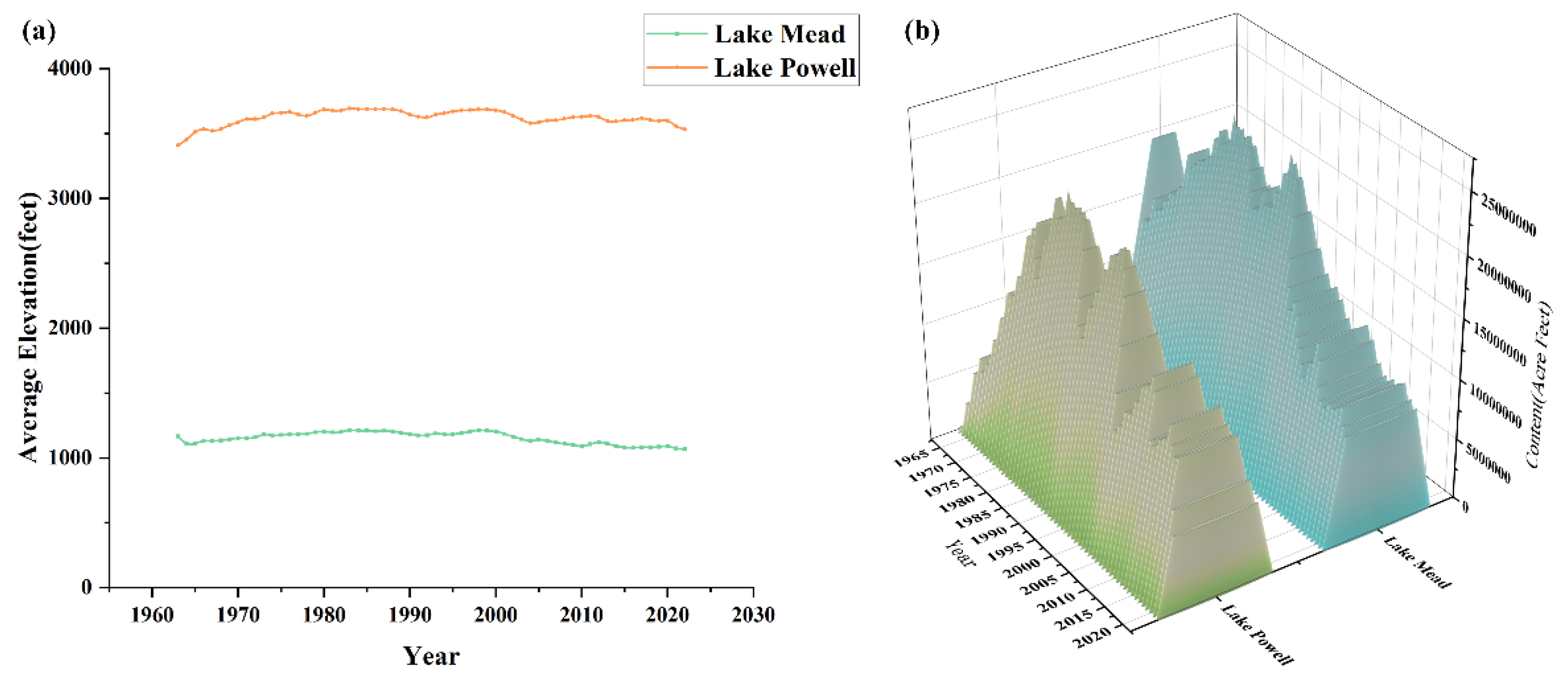
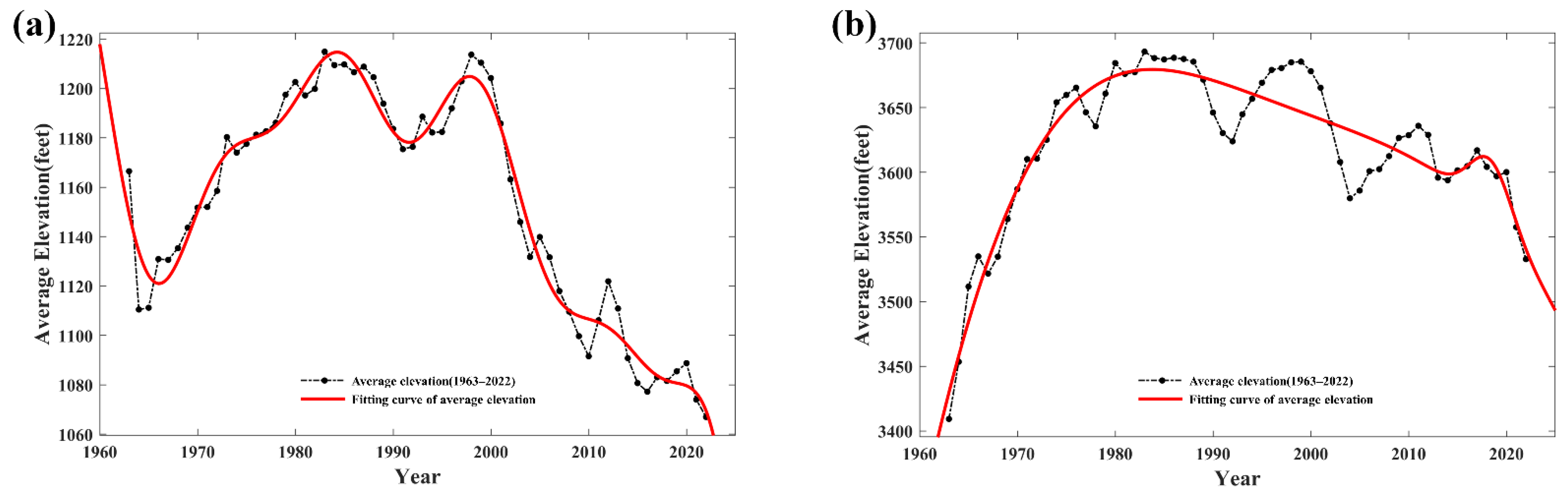
The water level of Lake Mead and Lake Powell from 1963 to 2022. (a) The average elevation. (b) The content. Source: National Water Information System https://waterdata.usgs.gov/nwis (accessed on 20 January 2022).
Figure 8.
The water level of Lake Mead and Lake Powell from 1963 to 2022. (a) The average elevation. (b) The content. Source: National Water Information System https://waterdata.usgs.gov/nwis (accessed on 20 January 2022).

Figure 9.
Contour topographic map of two dams and their surroundings. Source: topographic-map https://en-us.topographic-map.com (accessed on 20 January 2022).
Figure 9.
Contour topographic map of two dams and their surroundings. Source: topographic-map https://en-us.topographic-map.com (accessed on 20 January 2022).

Figure 10.
Schematic of distribution under extreme conditions, idealized state.

Figure 11.
Reservoir average annual elevation statistics and nonlinear fitting map from 1963 to 2022. (a) The HD. (b) The GCD. Source: National Water Information System https://waterdata.usgs.gov/nwis (accessed on 20 January 2022).
Figure 11.
Reservoir average annual elevation statistics and nonlinear fitting map from 1963 to 2022. (a) The HD. (b) The GCD. Source: National Water Information System https://waterdata.usgs.gov/nwis (accessed on 20 January 2022).

Figure 12.
The Results of Fitting and Predicting of the Water Elevations at the dam. (a) The HD. (b) The GCD.
Figure 12.
The Results of Fitting and Predicting of the Water Elevations at the dam. (a) The HD. (b) The GCD.

Figure 13.
Volume of water to be introduced at the HD and the GCD.

Figure 14.
Particle swarm algorithm vector demonstration map.

Figure 15.
Particle swarm algorithm vector demonstration map.

Figure 16.
Percentage of U.S. Electricity Generation of four main types.

Figure 17.
The results of sensitivity analysis of the dam water level prediction model. The blue line in the figure is the standard fit curve. The red line shows the curve obtained by slightly increasing the parameters. The yellow line shows the curve obtained after the parameters are slightly reduced. (a) The HD. (b) The GCD.


Table 1.
The population and electricity consumption analysis in five states. Source: State Profile and Energy Estimates https://www.eia.gov/state/ (accessed on 20 January 2022).
Table 1.
The population and electricity consumption analysis in five states. Source: State Profile and Energy Estimates https://www.eia.gov/state/ (accessed on 20 January 2022).
| State | Population (Thousands) | Per Capita Electricity Consumption (kWh) |
|---|---|---|
| AZ | 6600 | 80 |
| CA | 40,000 | 100 |
| WY | 6000 | 75 |
| NM | 2080 | 50 |
| Co | 5500 | 60 |
Table 2.
Assignment of four major attributes to selected counties in five states. Only the first three and the last two are excerpted here.
Table 2.
Assignment of four major attributes to selected counties in five states. Only the first three and the last two are excerpted here.
| GeoFips | GeoName | Population | Gross Agricultural Product | Gross Industrial Product | HD Score | GCD Score |
|---|---|---|---|---|---|---|
| 04001 | Apache, AZ | 71,875 | 20,288 | 2,137,179 | 9 | 9 |
| 04003 | Cochise, AZ | 127,450 | 156,199 | 4,345,417 | 4 | 4 |
| 04005 | Coconino, AZ | 142,481 | 25,092 | 6,296,249 | 9 | 10 |
| 8123 | Weld, CO | 333,983 | 2,180,483 | 18,780,994 | 2 | 3 |
| 8125 | Yuma, CO | 10,047 | 547,401 | 863,551 | 1 | 2 |
Table 3.
Relative proximity of each county. Only the first three and the last two are excerpted here.
Table 3.
Relative proximity of each county. Only the first three and the last two are excerpted here.
| Hoover Dam | Glen Canyon Dam | |||
|---|---|---|---|---|
| Rank | County | Relative Proximity | County | Relative Proximity |
| 1 | Los Angeles, CA | 0.712775407 | Los Angeles, CA | 0.71267 |
| 2 | Maricopa, AZ | 0.378339863 | Maricopa, AZ | 0.378134 |
| 3 | Santa Clara, CA | 0.339296864 | Santa Clara, CA | 0.339103 |
| 192 | Niobrara, WY | 0.002777699 | Del Norte, CA | 0.002777699 |
| 193 | Weston, WY | 0.002001377 | Trinity, CA | 0.002001377 |
Table 4.
The scheme of compensation for Mexico.
| Percentage of Water Deficit below Standard | Compensation Price |
|---|---|
| Less than 20% | p |
| 20~40% | 1.5p |
| 40~60% | 3p |
| 60~80% | 6p |
| More than 80% | 12p |
Publisher’s Note: MDPI stays neutral with regard to jurisdictional claims in published maps and institutional affiliations. |
© 2022 by the authors. Licensee MDPI, Basel, Switzerland. This article is an open access article distributed under the terms and conditions of the Creative Commons Attribution (CC BY) license (https://creativecommons.org/licenses/by/4.0/).
Share and Cite
MDPI and ACS Style
Zhang, Q.; Fan, M.; Hui, J.; Huang, H.; Li, Z.; Zheng, Z. Smart Sharing Plan: The Key to the Water Crisis. Water 2022, 14, 2320. https://doi.org/10.3390/w14152320
AMA Style
Zhang Q, Fan M, Hui J, Huang H, Li Z, Zheng Z. Smart Sharing Plan: The Key to the Water Crisis. Water. 2022; 14(15):2320. https://doi.org/10.3390/w14152320
Chicago/Turabian StyleZhang, Qinyi, Mengchao Fan, Jing Hui, Haochong Huang, Zijian Li, and Zhiyuan Zheng. 2022. "Smart Sharing Plan: The Key to the Water Crisis" Water 14, no. 15: 2320. https://doi.org/10.3390/w14152320
Note that from the first issue of 2016, this journal uses article numbers instead of page numbers. See further details here.