
Influence of Selected Environmental Factors on Diatom β Diversity (Bacillariophyta) and the Value of Diatom Indices and Sampling Issues


1
Institute of Nature Conservation, Polish Academy of Sciences, Mickiewicza 33 Ave., 31-120 Cracow, Poland
2
Institute of Evolution, University of Haifa, Mount Carmel, Abba Khoushi Avenue 199, Haifa 3498838, Israel
*
Author to whom correspondence should be addressed.
Water 2022, 14(15), 2315; https://doi.org/10.3390/w14152315
Submission received: 11 June 2022
/
Revised: 15 July 2022
/
Accepted: 21 July 2022
/
Published: 26 July 2022
(This article belongs to the Special Issue Advances and Challenges of Lake Biodiversity)
Abstract
:Human impacts and environmental climate changes have led to a progressive decline in the diversity of diatoms in lakes in the recent past. The components of β diversity (e.g., species turnover and nestedness) and underlying factors are still poorly understood. Here, we report an investigation of two alternative approaches—beta diversity (β diversity) partitioning and local contribution to β diversity (LCBD)—including their responses to selected environmental factors and representativeness of samples in estimating the ecological fitness of a lake. The β diversity of diatoms and their local contributions could be explained by the effects of environmental variables (p < 0.01). The random forest method showed the most contribution to the variance for NO3−, Cl−, and SO42−. PERMANOVA as well as a network analysis in JASP (Jeffrey’s Amazing Statistics Program) showed significant differences between the seasons in diatom assemblages and in the diatom index for Polish lakes (IOJ). Our findings provide insights into the mechanisms responsible for community organizations along environmental gradients from the perspective of β diversity components, and mechanisms of the indication value of diatoms for lakes; the results could be used especially by countries implementing ecological assessments.
Keywords:
β diversity; turnover; nestedness; lakes; diatoms; diatom index for Polish lakes; Wigry National Park; Poland1. Introduction
The response of organisms to habitat loss is one of the most important directions of modern research. The destruction of the natural habitats of lakes is associated with a deterioration in water quality, reflecting a decline in the value of β diversity. Poor water quality is reflected in the values of diatom indices. The low quality of habitats is a threat to many aquatic species, although some can survive a degree of degradation. Understanding the mechanisms responsible for community organization along environmental gradients from the perspective of β diversity components is now a central issue in ecology and conservation biology [1]. β diversity, its components (e.g., species turnover and nestedness), and the underlying drivers remain poorly understood, even though β diversity plays an important role in explaining ecological processes, especially for cross-scale biodiversity patterns [2]. Studies of metacommunity processes as well as of β diversity and its components are gaining more and more attention [3]. An estimation of β diversity allows us to measure the differences between the communities present in every place, considering the identities of all the species [4]. It gives a unique opportunity for understanding different layers of environmental conditions and water quality. The β diversity proposed by the Balsega [5] framework is based on a presence-absence matrix and can be divided into the components of turnover (species replacement—one species replaces another with no change in species richness) and nestedness (diversity differences due to species gain or loss). A different approach framework proposed for analyzing β diversity, especially at the local scale, was developed by Legendre and De Cáceres [6] for matrices with a quantified species contribution (LCBD—local contribution to β diversity). The LCBD index can also be partitioned into replacement (equivalent to turnover) and nestedness. Species turnover/replacement is impacted by environmental filtering, competition, and historical events [7], while species nestedness is impacted by species thinning and other ecological processes (human impact, physical barriers, etc.) [8]. All these methods are useful in the analysis of habitat changes and environmental conservation.
The Water Framework Directive requires classifying all surface waterbodies according to their ecological status, and it gives us a more holistic view [9]. The state of waterbodies is examined so that a tipping point before serious deterioration can be caught and waterbody management can be thus implied [10]. Diatoms are considered to be among the best groups of biota used for waterbody assessments [11,12,13,14]. Diatom-based metrics show strong responses to nutrient gradients [15,16,17]. However, many countries, including Poland, still have problems with the successful implementation of diatom indices for lakes [18,19,20,21,22,23], and many others are also about to implement ecological indicators to their environmental inspections. Custom river indexes are used for many lake water assessments [18,20]. The diatom index for Polish lakes (IOJ) rarely specifies assessments other than very good or good; even less frequent are situations when the IOJ is responsible for the final evaluation [21,22,23]. Other biological elements show a more varied distribution [21,22,23]. Sources of imperfections in the diatom index of Polish lakes [24] were revised by Zgrudno et al. [25], making the method easier for users; however, many problems remain unresolved. For example, only one sample from a lake is required to be collected in one year in Poland. One sample per lake is consistent with the recommendations made by the authors of [26]—one sampling site distant from source of pollution is thought to be sufficient for the needs of water management. Many countries are testing phytobenthos more than once a year and using more than one sample per lake [18,27,28], so we hypothesized that one-time sampling from a lake may be a source of error in the field method. In support, some studies have shown differences in diatom assemblages within lake surveys [29,30,31,32,33]. The variability of phytobenthos communities is different for the studied lakes and is additionally related to the seasons of the year [31,32]. This variability is not always related to the availability of nutrients. The hydrological regime, light, temperature, and grazing practices also affect phytobenthos [10,34].
The aim of our research was to investigate the influence of the environmental factors of lakes on the β diversity of diatoms and the diatom index, and to assess the representativeness of one lake sample per year.
2. Materials and Methods
2.1. Study Area
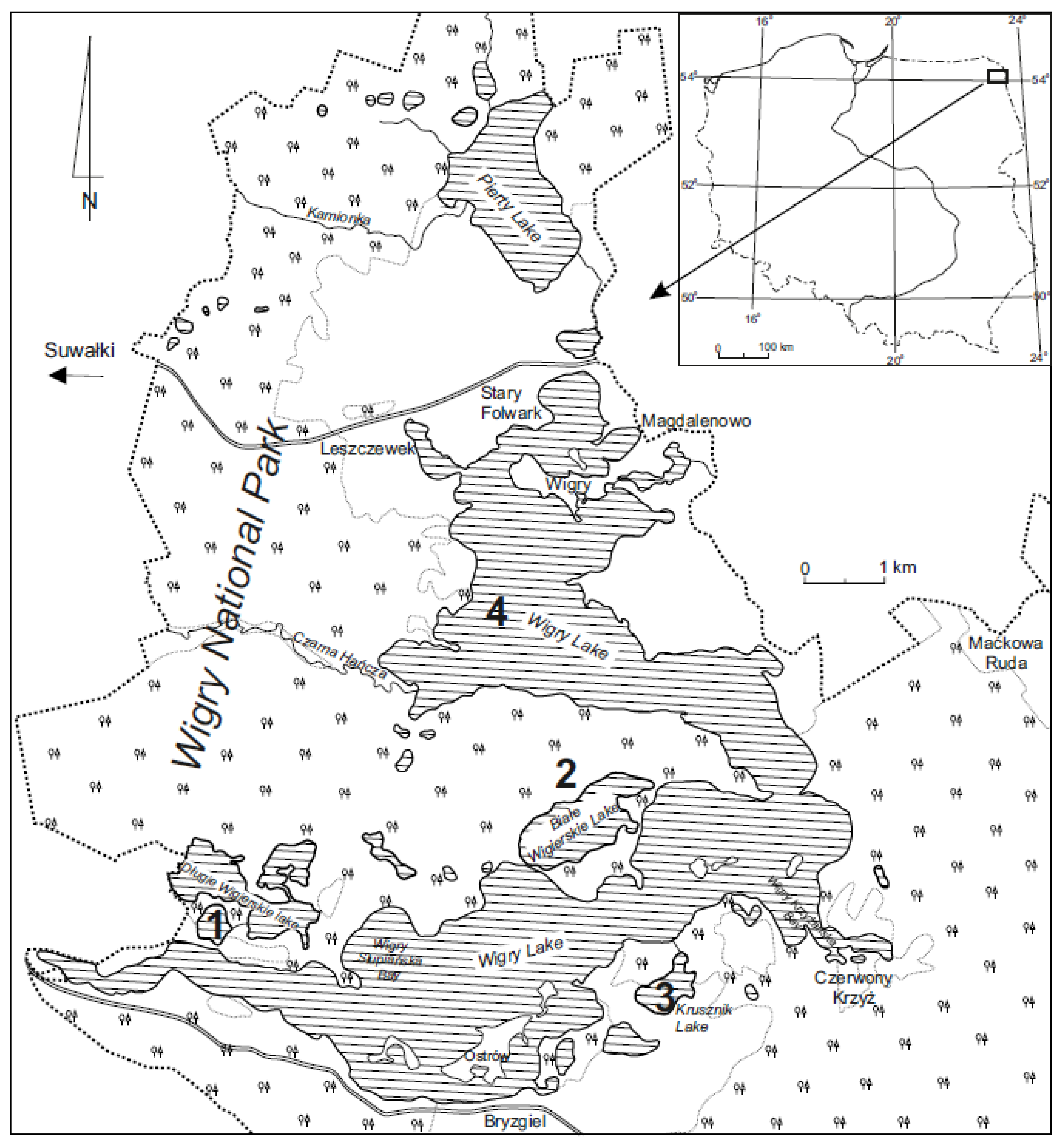
This study took place in Wigry National Park, in Northeast Poland, and included four lakes—Białe Wigierskie (BW), Krusznik (K), Okrągłe (O) and Wigry (W) (Figure 1, Table 1). The study area is under the influence of a temperate climate, transitional between the maritime and the continental [35,36]. The studied lakes are of glacial and postglacial origin and are remnants of the Weichselian glaciation [37]. The lakes differed in their limnological, physical, and chemical features (Table 1 and Table 2); however, they were all characterized by harmonic evolution. The biggest lake was Wigry—at 2163.3 ha—and the smallest was Okrągłe lake—at 13.7 ha. The direct catchment of these lakes also differed, despite the fact that they are all in National Park. Okrągłe and Wigry were more affected by human impact; on the other hand, Krusznik was impacted by extensive agriculture. The direct catchment of Białe Wigierskie lake was under strict protection. These differences gave us the opportunity to test the β diversity as well as the diatom index for Polish lakes (IOJ) for a relatively wide spectrum of variables, despite the small study area.
2.2. Chemical and Physical Data
In total, 48 water samples were analyzed for their physical and chemical properties. They were collected in autumn (October 2017), spring (May 2018), and summer (August 2018) from 12 sampling points (four in each lake). All the sampling for physical and chemical properties was done in open water, with comparable environments selected as much as possible. Conductivity and pH were measured using a YSI 6600 V2 multiparameter sonde. Water for the chemical analyses was sampled 20–30 cm below the lake surface using 0.33 L polyethylene bottles, and stored in the dark at 4 °C, to limit ongoing chemical reactions. Ionic analyses were related to PO43−, SO42−, NO3−, F−, CO32−, Cl−, and NO2−, as well as Na+, Li+, K+, Mg2+, NH4+, and Ca2+. Laboratory measurement were performed using the Dionex ion chromatograph at the laboratory of the Institute of Nature Conservation, Polish Academy of Sciences. Spatial differences in the shorezone were calculated using the shorezone functionality index manual [38].
2.3. Diatom Data
In total, 48 samples were analyzed. They were collected in autumn (October 2017), spring (May 2018), and summer (August 2018) from 12 sampling points (four in each lake). Samples of periphyton were taken from the common reed, Phragmites australis (Cav.) Trin. ex Steud. Samples were cleaned by adding 37% H2O2, and were then heated. The reaction was completed by adding KMnO4 and HCl. The cleaned diatom material dried on slides was mounted in Naphrax® synthetic resin. The slides were then analyzed using a Nikon Eclipse-80i microscope, with at least 400 diatom valves counted. Diatom identification mainly followed the procedures in [39,40,41,42,43]. Diatom indices (IOJ—diatom index for Polish lakes, Tj—trophic index, and GR—reference species index) were calculated using a program provided by the Polish Inspectorat of Environmental Protection (version 2010 and an updated version from May 2019) [24,25].
2.4. Statistical Data
2.4.1. β Diversity of Diatoms
Analyzed samples matrices were used to calculate β diversity [44]—(1) the total pairwise β diversity Sørensen dissimilarity index with partitioning (species turnover and nestedness) (betapart package R), and (2) local contribution to beta diversity (LCBD) with partitioning and species contribution to β diversity (SCBD) (adespatial package R). Data were cleaned before analysis—only species that had an abundance of at least 1% in 2 or more samples were used [33]—and were square-root-transformed to reduce the influence of very rare and abundant species on the diversity scores. In total, 6 β dissimilarity matrices were generated. Prior to the statistical analyses, all the abiotic variables were z-score-standardized (i.e., mean = 0, SD = 1) as well as log-transformed (if needed). Next, the chemical and physical variable distances among the samples were calculated (Euclidean distance). These matrices were transformed into a data frame and used for further analysis as distance-values. To quantify the association of each component of β diversity with the spatial and environmental factors, a multiple regression on the distance matrices ([45], MRM, Table 3) was used. To reduce the effect of spurious relationships between the variables, the MRM test was conducted with all the selected variables in the non-redundant variable sets. Then the non-significant variables from this initial MRM test were removed and the test was re-run. The significance of the partial regression was tested 999 times by a matrix permutation. The relationship between the β diversity indices in distance matrix and the selected variables was modelled using the random forest (RF) algorithm ([46] python 3.9 program—scikit learn 0.24 library). Optimal hyperparameters were found using a random search followed by a grid search (Table 4, with hyperparameters). The importance of each predictor variable (Table 4) was determined by: (1) permutation feature importance (rfpimp) [47], and (2) mean decrease accuracy (eli5) [48]. To reduce the effect of spurious relationships between variables, the RF model was developed with all the selected variables. Then, the variable(s) with the lowest contribution (less than 0.05) were removed and the model was re-developed until all contributed features were positive (add value) on the random forest model [47,48].
To examine the changes in β diversity across selected environmental factors, we divided the samples into groups, which were nested in lake factors and season factors, and for each sampling point in those nested conditions, arithmetic means were calculated. In this way, we generated a single-point matrix, taking into consideration that single-point measurements are more powerful and recommended for calculations [44]. The statistical dependence between the explanatory variables was assessed using Pearson’s correlation analysis and the variables with high correlation coefficients (Pearson R2 > 0.7) were excluded from the models. Then, the relationships between the environmental factors and β diversity metrics were explored with linear models. We performed variation partitioning analyses as well as an RDA analysis (redundancy analysis [49,50,51], Table 3) to check which of the β diversity indices better corresponded with chemical and physical water features.
2.4.2. Seasonal Differences, Between-Lake Differences, and Effectiveness of Indices
The differences between seasons were analyzed in 3 datasets: (a) diatom assemblages, (b) diatom indices, and (c) an assessment based on diatom index. To assess differences in diatom assemblages, a nonmetric multidimensional scaling analysis was conducted (NMDS, [52]) based on the Bray-Curtis similarity matrix ([53], R 4.0.2 software, packages: vegan, plot3D). Data were cleaned before the analysis—only species which had an abundance of at least 1% in 2 or more samples were used [33]—and were square-root-transformed to reduce the influence of very rare and abundant species on ordination scores. In order to analyze the variability in the studied lakes, the datasets from the four lakes were ordered in a bidimensional space using the above-mentioned NMDS with Bray-Curtis as a dissimilarity measure [32,33]. Significant differences between the centroids of the multivariate areas covered by the four lakes were tested with PERMANOVA (permutational analysis of variance [54]) and interpreted as indicative of differences in the mean composition of diatom assemblages, diatom indices (IOJ), and assessments based on diatom indices among lakes (assessment based on IOJ) (R software, vegan package). PERMANOVA was performed to assess statistical differences between seasons and lakes: in diatom assemblages (Euclidean distance matrix [32] and parallel to the methods of [33] using NMDS), and in diatom indices and assessments based on a diatom index (R software, vegan package, pairwise adonis package). A test of the homogeneity of multivariate dispersion [55] was also applied to assess whether cells (groups of points nested in lake and season) (batadisper, R, vegan) had a similar dispersion (homogeneity of variance—equivalent to Levene’s test). A correlation analysis was performed as the network analysis in JASP (Jeffrey’s Amazing Statistics Program) [56,57] on the botnet package in R statistical software. The line thickness among stations reflected the correlation value (only significant correlations were represented); blue was positive, and red was negative. The nodes were positioned using the Fruchterman-Reingold algorithm, which organizes the network based on the strength of the connections between nodes. JASP network graphs were constructed on the base of each revealed species abundance, number of bioindicators, and environmental data in each lake and for each of the four seasons.
We used RDA ([49,50,51], R software, vegan package) to assess which of the diatom indices explained more of variance in the environmental dataset. Prior to reducing skewness and normalizing distributions for the data analyses, all physical and chemical variables were log-transformed when necessary, and all variables were normalized. Data were cleaned to avoid multicollinearity—the most correlated variables were excluded from analysis [32]. Characteristic species for every lake were revealed by IndVal [58].
2.5. Spatial Diversity
The representativeness of the samples was investigated by the comparison of original samples with Monte Carlo-simulated assemblages [32,33,51]. In order to simulate assemblages, specimens from the same lake in the same season were pooled and 1000 new samples for each were drawn at random (400 specimens per sample) [32,47,51]. Data sets were square-root-transformed and a PCoA (principal coordinate analysis [59]) using Bray-Curtis as a dissimilarity measurement was performed on each randomized dataset separately (R, package stats) and then plotted. The distribution was used to detect the representativeness of original species assemblages. Spatial within-lake variability was also assessed through comparing the Euclidean distance of original assemblages to the centroid of generated assemblages (simulated mean assemblages in PCoA). Boxplots were drawn to visualize differences. Samples with a distance to centroid that were located in the tail representing less than 5% were interpreted as poorly representative [51]. For comparison, there was a plotted cumulative PCoA plot for all simulated samples, with real samples highlighted. Simulated assemblages were also used for the calculation of the generated diatom index for Polish lakes (IOJ) (version 2010 and 2019) and assessments based on the diatom index. Distributions were visualized on histograms and on box-plots by comparing the Euclidean distance between the original dataset and the mean. General linear models were used to assess statistical differences between diatom assemblages and diatom indices in seasons and lakes. Samples with IOJ that were placed in the histogram tails representing less than 2.5% were interpreted as poorly representative.
3. Results
3.1. β Diversity
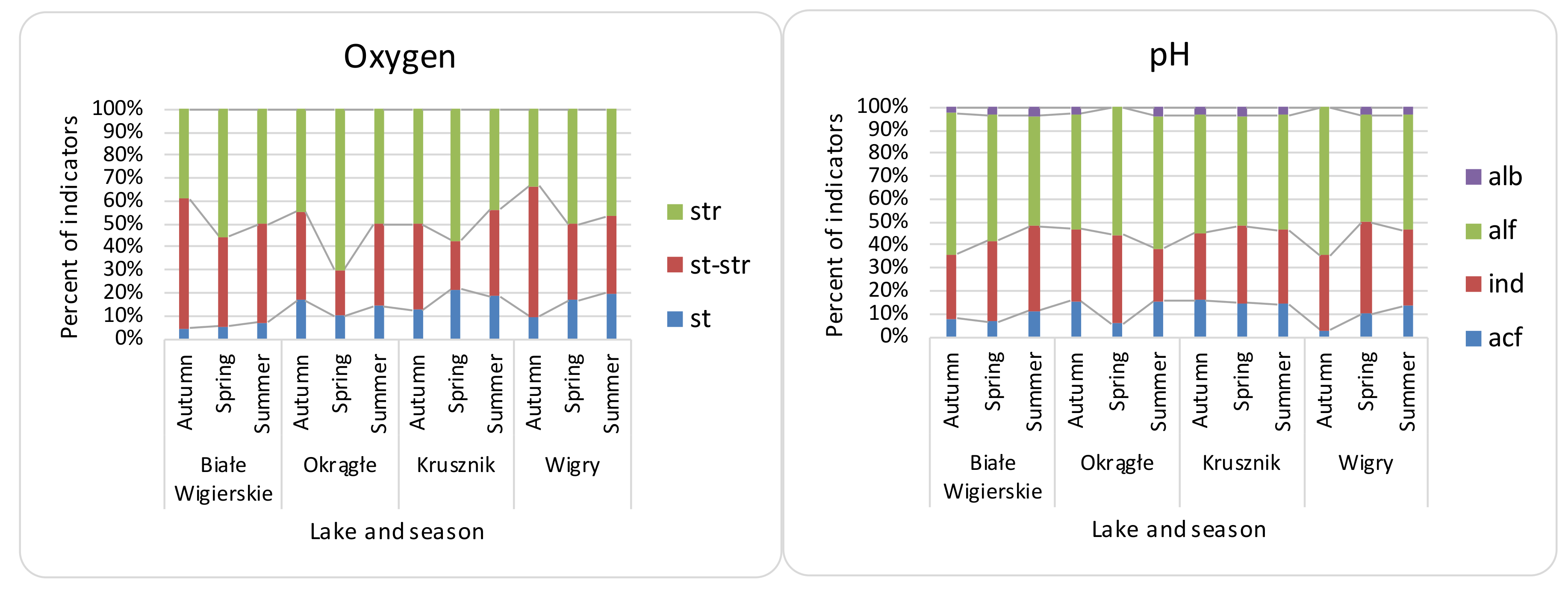
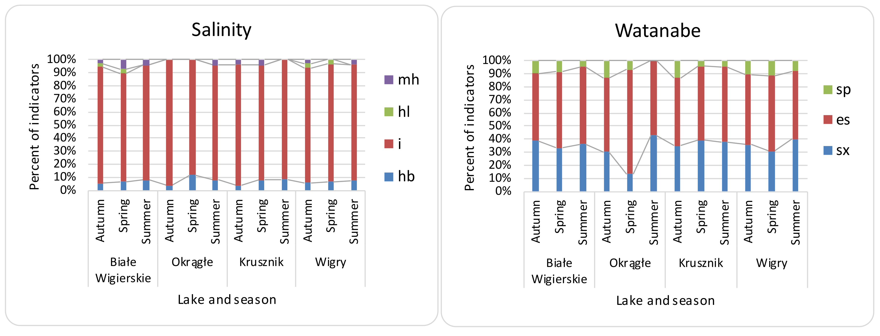
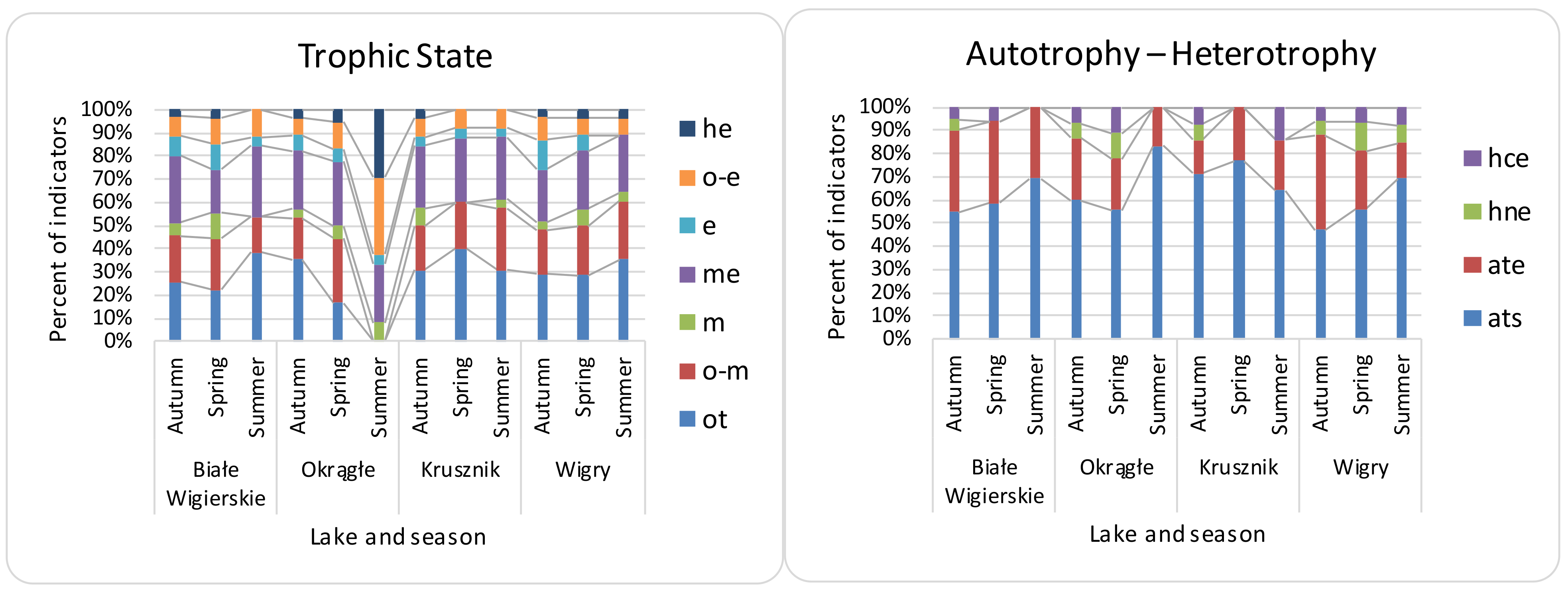
β diversity was mostly consistent with the turnover partition (mean—81%, median—85%), and nestedness on average had a 19% share (median—15%). Local contributions to the β diversity were mostly due to turnover partition (mean—88%, median—92%), which were higher than the nestedness (mean 11%, median—7%). The RDA showed a significant relationship between the environmental features for all β diversity indices, although with low explanation power (Table 3). The variation partitioning (Table 3) analysis gave the highest explanation power to NO3− and SO42− for β Sørensen indices (β Sørensen total adjusted R2 for NO3−—0.46, for SO42−—0.17; β Sørensen turnover adjusted R2 for NO3−—0.14; β Sørensen nestedness adj R2 for NO3−—0.20, for SO42−—0.34). The LCBD showed lower variation explanation, and PO43− had the most significant contribution. The MRM analysis (Table 3) showed NO3− as a significant contributor to the LCBD and β Sørensen, but the explanation power was not noticed for LCBD nestedness. β Sørensen nestedness showed a correlation only with Ca2+ ions. The explanation powers for all distances (in MRM) were much lower than for the raw material analysis (random forest and linear models). Random forest (Table 4) showed the greatest contribution to the variance for NO3−, Cl−, and SO42− to β Sørensen as well as LCBD; similar results were noticed for turnover. However, for nestedness, the components Ca2+ and NH4+ had the greatest contribution. Linear models (Table 4) showed higher R2: 0.26 for LCBD and 0.50 for β Sørensen. SO42− and NO3− had the highest contribution to both β Sørensen and LCBD. The turnover was the most significant process, as shown for both the LCBD and β Sørensen indices. For SCBD, the most significant species were Achnanthidium affinis, Brachysira neoexilis, and Cymbella affiniformis. The most characteristic taxa for the analyzed lakes were: BW—Gomphonema procerum, Encyonema ventricosum, and Nitzschia lacuum; OK—Nitzschia palea; K—Brachysira neoexilis, B. procera, and Eunotia arcubus; Wigry—Cymbella excisa, Fragilaria subconstricta, and Cocconeis placentula (Table 5). The samples included mostly benthic diatoms, with low numbers of plankto-benthic species. The present diatom indicator taxa have mostly temperate temperature preferences (e.g., Cymbella cymbiformis) with the addition of eurythermic taxa. Oxygen (Figure 2) indicators (e.g., Gomphonema vibrio) showed high seasonal differences, with the highest contribution of well-oxygenated water in the spring and the lowest in autumn. Salinity (e.g., halophobes—Cymbella proxima) (Figure 3) and pH indicators (e.g., alkaliphiles—Rhopalodia gibba) showed low differences across samples. The lowest amount of saproxenes (e.g., Delicata delicatula) and highest of saprophiles (e.g., Nitzschia palea) were observed in O lake. The lowest results were also observed in O lake for the trophic state (Figure 4) (e.g., nitrogen autotrophic—Gomphonema vibrio).
3.2. Seasonal Differences, Differences between Lakes, and Effectiveness of Indices
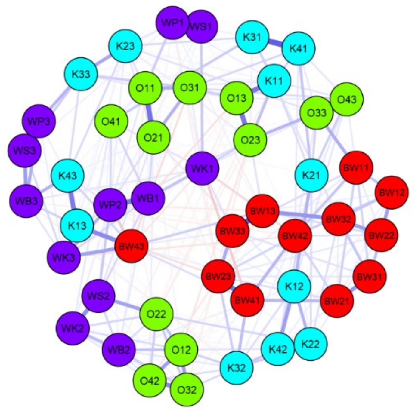
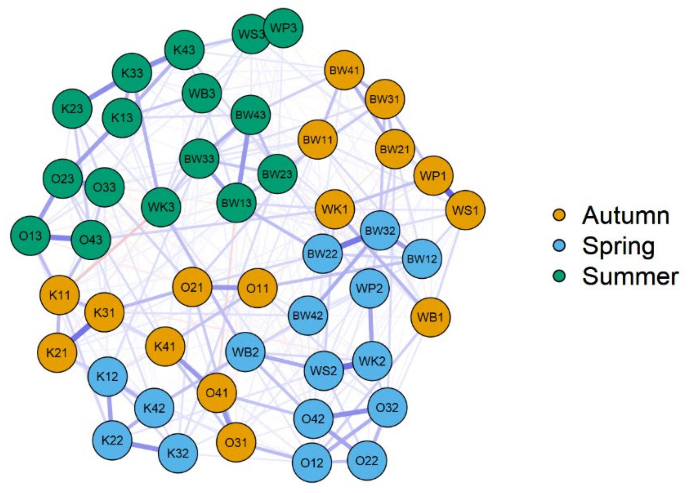
The diversity of the studied lakes is included in the values of physical and chemical parameters (Table 2). The conductivity ranged between 131 and 378 μS/cm; in general, WK and WB had the highest values, and BW had the lowest. A JASP comparison of the similarity of diatom assemblages, ecological indicators, and environmental data from the studied lakes is presented in Figure 5 and Figure 6. The JASP network plot shows that the BW assemblages were most similar (significant, p < 0.05); they formed one core with some of the K samples. The samples from other lakes were mostly divided into two cores (Figure 6). Season was an important differentiator for samples (Figure 6). The summer samples formed a distinctive core of similarity; the autumn and spring samples were more similar to each other. Overall, JASP showed that the analyzed lakes belonged, to some extent, to the same region with common climatic and landscape parameters. The most distinctive lake was W, as its samples were spread across clusters with a low correlation to each other.
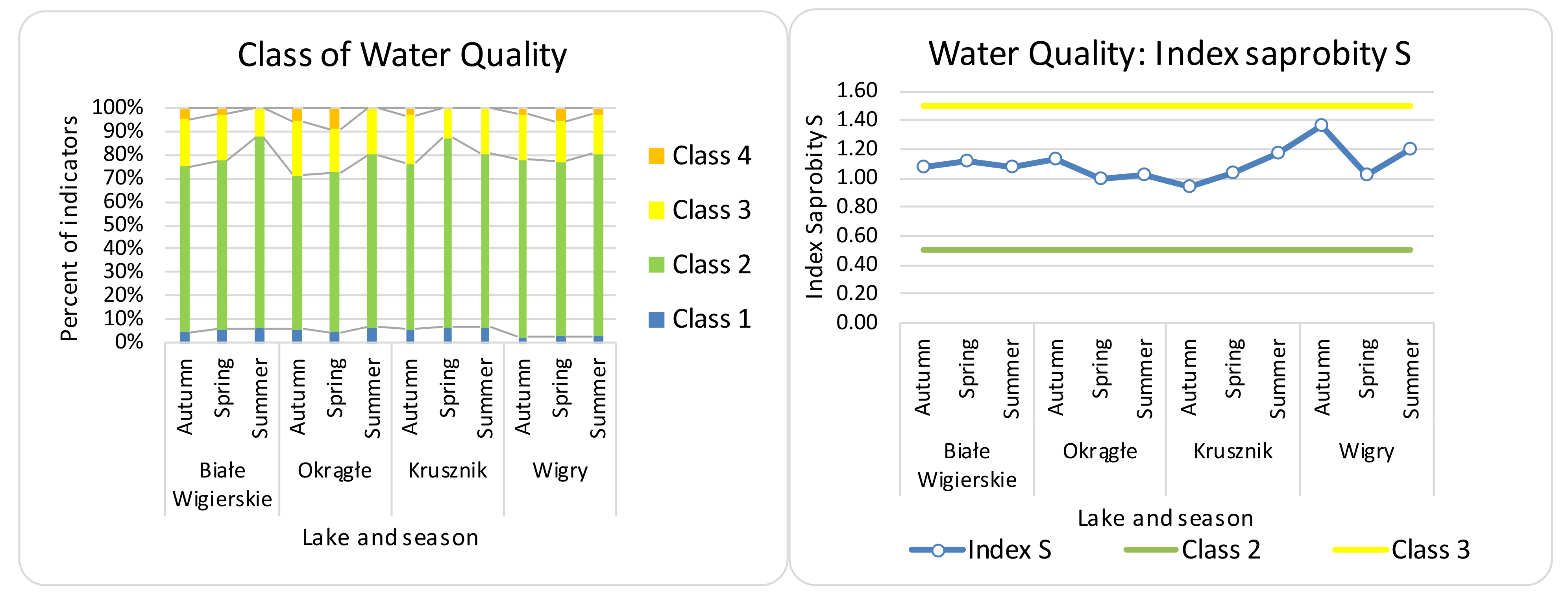
The most abundant species was Achnanthidium minutissimum, and it was dominant within most samples (87% of samples had more than 10% abundance; the range was 5–88%). An NMDS on the cleared abundance data with 1000 permutations was performed. As the stress in the 2D analysis was above 0.2, the NMDS was re-run in 3D (stress reached—0.16). A dissimilarity matrix obtained from the NMDS was used to analyze the differences between lakes and seasons (this procedure was chosen as the most suitable for data in studies such as [32,33]). A PERMANOVA global test showed significant differences in the abundance data between seasons and lakes (pseudo F = 9.6392, p < 0.001 for lakes; pseudo F = 7.6568, p < 0.001 for seasons). All four lakes and three seasons were significantly different (p < 0.05). The IOJ, version 2010, ranged between 0.688 for WP and 0.939 for BW, and the version from 2019 ranged between 0.66 for WP and 0.94 for BW. The class of water quality and index of saprobity showed mostly second-class indicators (Figure 7). The PERMANOVA test showed significant differences in the IOJ between lakes and seasons for IOJ versions 2010 and 2019 (for 2010: pseudo F = 3.9, p < 0.01 for lakes, and pseudo F = 4.05, p < 0.05 for seasons; for 2019: pseudo F = 3.9, p < 0.02 for lakes). Pairwise tests showed significant differences for 2010 between K and BW, K and W, summer and autumn, and autumn and spring; for 2019 between K and BW and between K and W, with no significant differences between seasons.
PERMANOVA showed differences in the assessments between lakes for the 2010 version (pseudo F = 7.8571, p < 0.002), but non-significant differences between seasons for the 2010 version and between lakes and seasons for the 2019 version. PERMANOVA showed non-significant differences between IOJ 2010 and IOJ 2019 and non-significant differences for the assessments.
We used an RDA to assess which of the diatom indices explained more of the variance in the environmental dataset. The RDAs used to model the variation in cleared and normalized nutrient levels, compared to the diatom indices and assessments used as predictors, showed significant explanation power for version 2010 (variance = 0.54, residuals = 8.47, p = 0.032, paxis = 0.038) and non-significant explanation power for IOJ version 2019 and both assessments.
3.3. Spatial Diversity
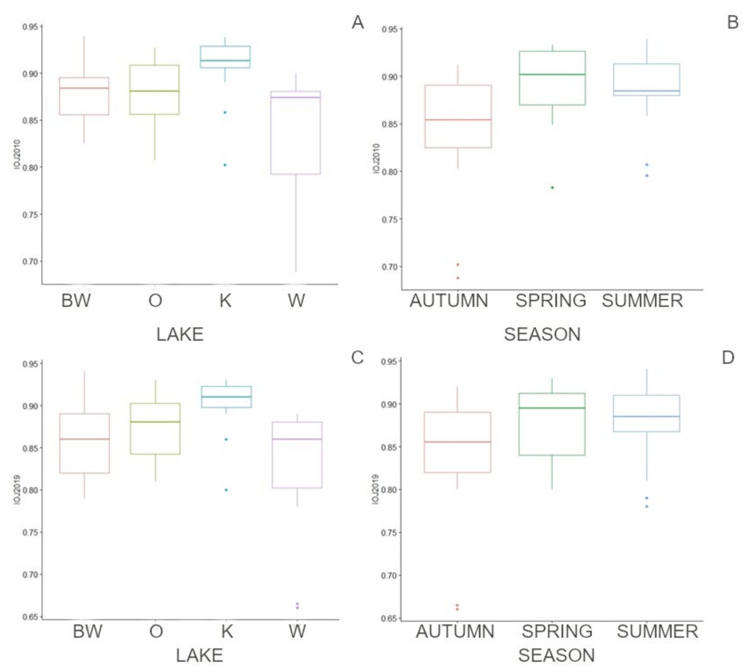
Monte Carlo-simulated assemblages were plotted using PCoA; real samples were highlighted (Figure 8). The centroids generated in the PCoA for each separately simulated data set were interpreted as mean assemblages and used to calculate the distances to this assembly. GLM tests were performed to compare the representativeness of samples for lakes and seasons; the results showed significant differences between lakes (BW-K p = 0.015, W-K p = 0.018) and no significant differences between seasons (Figure 9). A total of 79% of samples were poorly representative of the mean assemblages for lakes; however, most of the distances were less than 0.3, which indicated good representation [32,60].
The generated assemblages were used to calculate the IOJ version 2010 and 2019, histograms were used to plot the differences, and the real samples were highlighted. A total of 69% of the real samples were poorly representative of the IOJ of the mean assemblages for lakes for version 2010, and 73% for version 2019.
4. Discussion
4.1. β Diversity
Studies using variation partitioning to unravel metacommunity mechanisms assume that, in general, (I) species-sorting—if solely the “environmental variables” fraction—significantly explains the community structures; (II) neutral theory or patch dynamics—if only the “spatial variables” fraction—is significant; and (III) the mass-effect concept or the combination of species-sorting and mass-effect, if both fractions have significant explanatory power [61]. In our case, β diversity was mainly constructed with species turnover and was highly driven by environmental changes, with no statistically significant changes in the spatial factors represented by SFI; the filtering effect of the lakes’ local environmental characteristics and species sorting played a significant role (Table 3 and Table 4). Our results correspond well with the data presented by Epele et al. [62]. The variables with the most explanation power were NO3− and SO42−, both being indicators of water eutrophication and human impact on the environment [63]. Higher concentrations as well as differences in NO3− and SO42− resulted in the highest species turnover as well as species nestedness; however, the turnover contribution was more powerful in the tested variance. The LCBD showed a lower variation explanation than the β Sørensen indices. These findings are consistent with research where LCBD β diversity was not well-determined by the local environmental characteristics [3]. A high dominance in the studied lakes contributed to lower LCBD values in comparison to the presence-absence β Sørensen indices. The distance analysis was less powerful than the single-value analysis, which is consistent with [44]. However, in our case random forest successfully showed similar patterns for distance matrices, similarly to the linear regression model.
The species with the highest incidence based on SCBD were Achnanthidium affinis, Brachysira neoexilis, and Cymbella affiniformis. These taxa are relatively common; however, they are not the most abundant ones. This score is comparable to the results shown by Szabó et al. [3]. The most common taxa are present in most of the samples, so they have little effect on the β diversity; on the other hand, species that are relatively common have high turnover, which contributes to overall β diversity. This mechanism is consistent with our findings that the most common taxa did not contribute to β diversity, and as well, they skewed the indication analysis. The presence-absence data underweighted those taxa so that the overall explanation power rose in the β Sørensen indices. Higher LCBD values were seen in samples with high or low species richness [1]. The high LCBD index could be a result of special ecological conditions, which should be given more attention in terms of conservation [8].
4.2. Spatial and Seasonal Differences
Seasonal differences between diatom assemblages were reported numerous times; however, whether these differences were caught by ecological assessments remains mostly unknown, especially for the diatom index for Polish lakes. Our results show significant differences in the qualitative composition of diatom assemblages occurring in individual seasons and in the diatom index for Polish lakes (IOJ) (continuous variable, 0–1); however, an ecological assessment performed using IOJ 2010and 2019 (very good, good, moderate, poor, bad) showed no significant differences between the seasons. More samples per year gave us redundant information about the ecological status (very good, good, moderate, poor, bad) despite significant differences between assemblages and the IOJ itself (continuous variable, 0–1). Elias et al. [31] reported similar results for streams and IPS assessments. Diatoms are naturally spatially and seasonally dynamic [31,33]. However, many species exhibit a similar response to the environment, and despite taxonomical differences, assessments remain comparable. The spatial differences within lakes were mostly lower than a distance of 0.3 to the centroids based on a PCoA performed on Monte Carlo-generated assemblages [32,59]. If the average composition of diatom assemblages significantly differs between two lakes with contrasting environmental characteristics, then single samples can be faithfully used for environmental bioindication, provided the environmental variable of interest explains a significant portion of the diatom variance [32]. If that is not the case, and the diatom composition between-lake variance is lower than the within-lake variance, then the number of single samples needed to represent the environmental differences among lakes is highly dependent on the sampling design [32,51]. In our analysis, the between-lake variance was far greater than the within-lake variance. These results indicate a good representation of lake samples. The IOJ ecological assessments mostly were not differentiated within a lake, despite the fact that over 65% of the IOJs (continuous variable, 0–1) calculated for real samples were considered as poor representations of the lake. The border lines between the ecological assessment groups were so wide that different IOJs gave similar assessments. More samples per lake and more samples per year seemed to give redundant information about the ecological status, especially for current assessment borders. Prygiel et al. [64] and Kelly et al. [10] have suggested that the uncertainty due to the sampling process itself is relatively small in comparison to other sources, such as, for example, taxonomic issues. Kelly et al. [10] have suggested that more reliable information would be given by more samples over a longer period (not seasonally, but in different hydrological years). Rimet et al. [34] and Marzin et al. [65] reported for their studies that spatial factors play a very limited role; on the other hand, water currents, animals, winds, and humans play intense roles in the diversity of diatoms at regional scales.
Diatoms have been used to assess the ecological status of lakes for years; however, from the early stages of implementing diatom indices in lakes to the current time, researchers have reported problems with the most abundant species such as Achnanthidium minutissimum [66,67]. A dominance of A. minutissimum is reported in many lakes, such as deep lakes with low to medium alkalinity [63]. Achnanthidium minutissimum is described as a pioneer species, so small disturbances such as water fluctuation, wind, or grazing will favor this species. However, A. minutissimum is a dominant species even in water reservoirs that have been severely impacted by metal contamination [68]. On the other hand, more severe disturbance, which impact grazing organisms, favor a more even structure of the assemblages [69]. Kelly et al. [16] showed that this process occurs on the moderate-to-good border of ecological assessments, and that diatom richness gives a unimodal response. However, we did not observe that this kind of assemblage difference caused such differences in the ecological assessment based on the IOJ. Moreover, we observed that less affected, mesotrophic lakes had a more even structure [70] compared to eutrophic lakes with high dominance, similarly to what has been reported by Stenger-Kovács et al. [71].
Some researchers have evaluated indices by checking how two indices react to differences in water chemistry (e.g., [72]). We evaluated two indices: version 2010 IOJ, and the updated version 2019. As we found, the grouping of hard-to-identify species into complexes using the updated 2019 version of IOJ gave us non-significant relationships with water chemistry, in comparison to significant relationships between the physical and chemical variables of water using the 2010 version. This is consistent with the findings of other research groups [73], as more taxonomic effort gives better results in terms of an indication of water chemistry changes. This aspect is important, especially for countries implementing ecological assessments and for those looking to simplify environmental inspections. We suggest that there is a high risk of losing useful data through this simplification. However, it is worth mentioning that both versions of IOJ had a low capacity for detecting environmental changes (R2 < 0.25, [74]).
Diatoms have proven to be useful indicators of water quality. Because of their short generation time, they give information in short time frames [18]. It is useful to collect such fast-paced changes in the environment. These abilities show that phytobenthos and macrophytes, even though they are both producers, do not give redundant information and should be used in parallel. A healthy ecosystem is a good indicator that a water body is being exploited in sustainable manner [75]. The results of the calculations of the diatom index for Polish lakes in recent years have not been well-received [21,22,23]. However, in this shape and form, the IOJ does not indicate problems with an ecosystem [22]. Unfortunately, more spatial and seasonal samples are not the answer we are looking for. An analysis of all the phytobenthos groups (as performed by Kelly in [69]), exclusion of the most dominant species (as performed by Szczepocka et al. in [67]), assembling species into functional groups, or other approaches [33,76] are possibly the next options to consider. More taxonomic effort has proven to increase the indication accuracy [73]; however, due to hardware and human resource shortages in provincial inspectorates of environmental protection, we do not recommend it.
5. Conclusions
The β diversity of diatoms and their local contributions can be explained by the effects of environmental variables—a total of 49.9% and 26.0% of diatom variance was explained respectively (p < 0.01) with no significant effect of spatial differences represented by SFI. In our analysis, we found that both versions of IOJ (2010 and 2019) had a low capacity for detecting environmental changes. The grouping of hard-to-identify species into complexes in the updated version of IOJ 2019, which is useful for practical reasons, gave us a non-significant relationship for water chemistry, in comparison to a significant relationship between the physical and chemical variables of water by using the 2010 version. As real samples and Monte Carlo-generated samples were mostly at a PCoA distance of 0.3 from the centroids, one sample per lake and per year seems sufficient and is a compromise between sampling effort and financial cost, especially taking into consideration resampling in longer periods of time (i.e., once a year). However, we recommend changes to the IOJ itself, due to its low explanation power and low sensitivity to environmental changes. Species with high dominance in lakes lower the indication capabilities of IOJ as well as the percentage contribution to β indices (LCBD). Our findings provide insights into the mechanisms responsible for community organization along environmental gradients from the perspective of β diversity components and the mechanisms of indication values of diatoms for lakes, and can be used especially by countries implementing ecological assessments.
Author Contributions
Conceptualization, methodology, software, validation, visualization, formal analysis, investigation, M.E.-K.; software—JASP, visualization, formal analysis, S.B.; original draft preparation, M.E.-K. and A.Z.W. All authors have read and agreed to the published version of the manuscript.
Funding
This work was supported by the Institute of Nature Conservation, Polish Academy of Sciences (Kraków, Poland), through grant funding for PhD students and through the Institute’s statutory funds.
Institutional Review Board Statement
Not applicable.
Informed Consent Statement
Not applicable.
Data Availability Statement
The data that support the findings of this study are available from the corresponding author upon reasonable request.
Acknowledgments
We are indebted to Hanna Szymańska, Hanna Werblan-Jakubiec, Bożena Zakryś, and Włodzimierz Winiarski, as well as employees of Wigry National Park, especially Mateusz Danilczyk, Maciej Romański, Mariusz Szczęsny, Lech Krzysztofiak, Maciej Kamiński, and Adam Flis. We are thankful for their generous help with field work and for other assistance. We thank Gary Hynes for the linguistic proofreading. We thank Wojciech Krztoń, Łukasz Peszek, and Matusz Rybak for their help and fruitful suggestions. We thank the anonymous Reviewers and Editors for their constructive suggestions and help.
Conflicts of Interest
The authors declare no conflict of interest.
References
- Wu, K.; Zhao, W.; Li, M.; Picazo, F.; Soininen, J.; Shen, J.; Zhu, L.; Cheng, X.; Wang, J. Taxonomic Dependency of Beta Diversity Components in Benthic Communities of Bacteria, Diatoms and Chironomids along a Water-Depth Gradient. Sci. Total Environ. 2020, 741, 140462. [Google Scholar] [CrossRef] [PubMed]
- Maloufi, S.; Catherine, A.; Mouillot, D.; Louvard, C.; Couté, A.; Bernard, C.; Troussellier, M. Environmental Heterogeneity among Lakes Promotes Hyper β-Diversity across Phytoplankton Communities. Freshw. Biol. 2016, 61, 633–645. [Google Scholar] [CrossRef]
- Szabó, B.; Lengyel, E.; Padisák, J.; Stenger-Kovács, C. Benthic Diatom Metacommunity across Small Freshwater Lakes: Driving Mechanisms, β-Diversity and Ecological Uniqueness. Hydrobiologia 2019, 828, 183–198. [Google Scholar] [CrossRef]
- Baselga, A.; Orme, C.D.L. Betapart: An R Package for the Study of Beta Diversity. Methods Ecol. Evol. 2012, 3, 808–812. [Google Scholar] [CrossRef]
- Baselga, A. Partitioning the Turnover and Nestedness Components of Beta Diversity: Partitioning Beta Diversity. Glob. Ecol. Biogeogr. 2010, 19, 134–143. [Google Scholar] [CrossRef]
- Legendre, P.; De Cáceres, M. Beta Diversity as the Variance of Community Data: Dissimilarity Coefficients and Partitioning. Ecol. Lett. 2013, 16, 951–963. [Google Scholar] [CrossRef]
- Specziár, A.; Árva, D.; Tóth, M.; Móra, A.; Schmera, D.; Várbíró, G.; Erős, T. Environmental and Spatial Drivers of Beta Diversity Components of Chironomid Metacommunities in Contrasting Freshwater Systems. Hydrobiologia 2018, 819, 123–143. [Google Scholar] [CrossRef] [Green Version]
- Legendre, P. Interpreting the Replacement and Richness Difference Components of Beta Diversity: Replacement and Richness Difference Components. Glob. Ecol. Biogeogr. 2014, 23, 1324–1334. [Google Scholar] [CrossRef]
- Nõges, P.; Poikane, S.; Cardoso, A.C.; van de Bund, W. Water Framework Directive the Way to Water Ecosystems Sustainability in Europe. LakeLine 2006, 21, 36–43. [Google Scholar]
- Kelly, M.; Bennion, H.; Burgess, A.; Ellis, J.; Juggins, S.; Guthrie, R.; Jamieson, J.; Adriaenssens, V.; Yallop, M. Uncertainty in Ecological Status Assessments of Lakes and Rivers Using Diatoms. Hydrobiologia 2009, 633, 5–15. [Google Scholar] [CrossRef]
- Dam, H.; Mertens, A.; Sinkeldam, J. A Coded Checklist and Ecological Indicator Values of Freshwater Diatoms from The Netherlands. Neth. J. Aquat. Ecol. 1994, 28, 117–133. [Google Scholar] [CrossRef]
- Hofmann, G.; Werum, M.; Lange-Bertalot, H.; Lange-Bertalot, H. Diatomeen im Süßwasser-Benthos von Mitteleuropa: Bestimmungsflora Kieselalgen für die Ökologische Praxis; über 700 der Häufigsten Arten und Ihre Ökologie; Gantner: Ruggell, Austria, 2011. [Google Scholar]
- Marra, R.C.; Algarte, V.M.; Ludwig, T.A.V.; Padial, A.A. Diatom Diversity at Multiple Scales in Urban Reservoirs in Southern Brazil Reveals the Likely Role of Trophic State. Limnologica 2018, 70, 49–57. [Google Scholar] [CrossRef]
- Cristóbal, G.; Blanco, S.; Bueno, G. (Eds.) Modern Trends in Diatom Identification: Fundamentals and Applications; Developments in Applied Phycology; Springer: Cham, Switzerland, 2020. [Google Scholar]
- Birk, S.; Bonne, W.; Borja, A.; Brucet, S.; Courrat, A.; Poikane, S.; Solimini, A.; van de Bund, W.; Zampoukas, N.; Hering, D. Three Hundred Ways to Assess Europe’s Surface Waters: An Almost Complete Overview of Biological Methods to Implement the Water Framework Directive. Ecol. Indic. 2012, 18, 31–41. [Google Scholar] [CrossRef]
- Kelly, M.; Urbanic, G.; Acs, E.; Bennion, H.; Bertrin, V.; Burgess, A.; Denys, L.; Gottschalk, S.; Kahlert, M.; Karjalainen, S.M.; et al. Comparing Aspirations: Intercalibration of Ecological Status Concepts across European Lakes for Littoral Diatoms. Hydrobiologia 2014, 734, 125–141. [Google Scholar] [CrossRef] [Green Version]
- Poikane, S.; Kelly, M.; Cantonati, M. Benthic Algal Assessment of Ecological Status in European Lakes and Rivers: Challenges and Opportunities. Sci. Total Environ. 2016, 568, 603–613. [Google Scholar] [CrossRef]
- Schaumburg, J.; Schranz, C.; Foerster, J.; Gutowski, A.; Hofmann, G.; Meilinger, P.; Schneider, S.; Schmedtje, U. Ecological Classification of Macrophytes and Phytobenthos for Rivers in Germany According to the Water Framework Directive. Limnologica 2004, 34, 283–301. [Google Scholar] [CrossRef] [Green Version]
- Poikane, S.; Birk, S.; Böhmer, J.; Carvalho, L.; de Hoyos, C.; Gassner, H.; Hellsten, S.; Kelly, M.; Lyche Solheim, A.; Olin, M.; et al. A Hitchhiker’s Guide to European Lake Ecological Assessment and Intercalibration. Ecol. Indic. 2015, 52, 533–544. [Google Scholar] [CrossRef]
- Kelly, M.G.; Chiriac, G.; Soare-Minea, A.; Hamchevici, C.; Juggins, S. Use of Phytobenthos to Evaluate Ecological Status in Lowland Romanian Lakes. Limnologica 2019, 77, 125682. [Google Scholar] [CrossRef]
- Bielczyńska, A. Bioindication on the Basis of Benthic Diatoms: Advantages and Disadvantages of the Polish Phytobenthos Lake Assessment Method (IOJ—The Diatom Index for Lakes)/Bioindykacja Na Podstawie Okrzemek Bentosowych: Mocne i Słabe Strony Polskiej Metody Oceny Jezior Na Podstawie Fitobentosu (IOJ—Indeks Okrzemkowy Jezior). Ochr. Śr. Zasobów Nat. 2015, 26, 48–55. [Google Scholar] [CrossRef] [Green Version]
- Ciecierska, H.; Kolada, A. ESMI: A Macrophyte Index for Assessing the Ecological Status of Lakes. Environ. Monit. Assess. 2014, 186, 5501–5517. [Google Scholar] [CrossRef] [Green Version]
- Wiech, A.K.; Marciniewicz-Mykieta, M.; Toczko, B. Stan Środowiska w Polsce. Raport 2018; Główny Inspektorat Ochrony Środowiska: Warsaw, Poland, 2018.
- Picińska-Fałtynowicz, J.; Błachuta, J. Przewodnik Metodyczny. Zasady Poboru i Opracowania Prób Fitobentosu Okrzemkowego z Rzek i Jezior; GIOŚ: Wrocław, Poland, 2010.
- Zgrundo, A.; Peszek, Ł.; Poradowska, A. Podręcznik Do Monitoringu i Oceny Rzecznych Jednolitych Części Wód Powierzchniowych Na Podstawie Fitobentosu; OceanSense Maciej Fojcik: Gdańsk, Poland, 2018. (In Polish) [Google Scholar]
- King, L.; Clarke, G.; Bennion, H.; Kelly, M.; Yallop, M. Recommendations for Sampling Littoral Diatoms in Lakes for Ecological Status Assessments. J. Appl. Phycol. 2006, 18, 15–25. [Google Scholar] [CrossRef]
- Lodewijks, P.; Brouwers, J.; Van Hooste, H.; Meynaerts, E. Energie-En Klimaatscenario’s Voor de Sectoren Energie En Industrie; MIRA 2009 Wetenschappelijk Rapport; Vlaamse Milieumaatschappij: Mechelen, Belgium, 2009; Available online: https://www.academia.edu/19642138/Energie_en_Klimaatscenario_s_voor_de_sectoren_Energie_en_Industrie (accessed on 1 June 2022).
- Charles, D.F.; Kelly, M.G.; Stevenson, R.J.; Poikane, S.; Theroux, S.; Zgrundo, A.; Cantonati, M. Benthic Algae Assessments in the EU and the US: Striving for Consistency in the Face of Great Ecological Diversity. Ecol. Indic. 2021, 121, 107082. [Google Scholar] [CrossRef]
- Picińska-Fałtynowicz, J.; Soszka, H. Fitobentos. In Ocena Stanu Ekologicznego Wód Zlewni Rzeki Wel. Wytyczne Do Zintegrowanej Oceny Stanu Ekologicznego Rzek i Jezior na Potrzeby Planów Gospodarowania Wodami w Dorzeczu; Wydawnictwo IRŚ: Olsztyn, Poland, 2011. [Google Scholar]
- Gołdyn, R.; Messyasz, B. Ocena Stanu Ekologicznego Jeziora Durowskiego w Roku 2013; Wydział Biologii Uniwersytetu im. Adama Mickiewicza w Poznaniu: Poznań, Poland. 2013. Available online: https://www.wagrowiec.eu/assets/files/dzialy/ochrona_srodowiska/dokumenty-do-pobrania/ocena-stanu/2018-stan-ekologiczny-jeziora-durowskiego.pdf (accessed on 1 June 2022).
- Elias, C.L.; Vieira, N.; Feio, M.J.; Almeida, S.F.P. Can Season Interfere with Diatom Ecological Quality Assessment? Hydrobiologia 2012, 695, 223–232. [Google Scholar] [CrossRef]
- Hassan, G.S. Within versus Between-Lake Variability of Sedimentary Diatoms: The Role of Sampling Effort in Capturing Assemblage Composition in Environmentally Heterogeneous Shallow Lakes. J. Paleolimnol. 2018, 60, 525–541. [Google Scholar] [CrossRef]
- Riato, L.; Leira, M. Heterogeneity of Epiphytic Diatoms in Shallow Lakes: Implications for Lake Monitoring. Ecol. Indic. 2020, 111, 105988. [Google Scholar] [CrossRef]
- Rimet, F.; Bouchez, A.; Montuelle, B. Benthic Diatoms and Phytoplankton to Assess Nutrients in a Large Lake: Complementarity of Their Use in Lake Geneva (France-Switzerland). Ecol. Indic. 2015, 53, 231–239. [Google Scholar] [CrossRef]
- Andrzejczyk, T.; Brzeziecki, B. The Structure and Dynamics of Old-Growth Pinus sylvestris (L.) Stands in the Wigry National Park, North-Eastern Poland. Vegetatio 1995, 117, 81–94. [Google Scholar] [CrossRef]
- Drzymulska, D.; Zieliński, P. Phases and Interruptions in Postglacial Development of Humic Lake Margin (Lake Suchar Wielki, NE Poland). Limnol. Rev. 2014, 14, 13–20. [Google Scholar] [CrossRef] [Green Version]
- Górniak, A. Current Climatic Conditions of Lake Regions in Poland and Impacts on Their Functioning. In Polish River Basins and Lakes—Part I.; Korzeniewska, E., Harnisz, M., Eds.; Springer International Publishing: Cham, Switzerland, 2020; Volume 86, pp. 1–25. [Google Scholar] [CrossRef]
- Nowicka, B.; Nadolna, A. Shorezone Functionality Index—Lake Charzykowskie Case Study. In Natural and Athropogenic Transformation of Lakes, Proceedings of the International Limnological Conference, Łagów Lubuski, Poland, 19–21 September 2012; Institute of Meteorology and Water Management: Poznań, Poland, 2012. [Google Scholar]
- Lange-Bertalot, H.; Hofmann, G.; Werum, M.; Cantonati, M.; Kelly, M. Freshwater Benthic Diatoms of Central Europe: Over 800 Common Species Used in Ecological Assessment; English edition with updated taxonomy and added species; Koeltz Botanical Books: Schmitten-Oberreifenberg, Germany, 2017. [Google Scholar]
- Wojtal, A.Z.; Ector, L.; Van de Vijver, B.; Morales, E.A.; Blanco, S.; Piatek, J.; Smieja, A. The Achnanthidium Minutissimum Complex (Bacillariophyceae) in Southern Poland. Algological Stud. 2011, 136–137, 211–238. [Google Scholar] [CrossRef]
- Lange-Bertalot, H.; Ulrich, S. Contributions to the Taxonomy of Needle-Shaped Fragilaria and Ulnaria Species. Lauterbornia 2014, 78, 1–73. [Google Scholar]
- Van de Vijver, B. Analysis of the Type Material of Navicula Brachysira Brébisson with the Description of Brachysira Sandrae, a New Raphid Diatom (Bacillariophyceae) from Iles Kerguelen (TAAF, Sub-Antarctica, Southern Indian Ocean). Phytotaxa 2014, 184, 139. [Google Scholar] [CrossRef]
- Delgado, C.; Novais, M.H.; Blanco, S.; de Almeida, S.F. Examination and Comparison of Fragilaria Candidagilae sp. nov. with Type Material of Fragilaria Recapitellata, F. Capucina, F. Perminuta, F. Intermedia and F. Neointermedia (Fragilariales, Bacillariophyceae). Phytotaxa 2015, 231, 1. [Google Scholar] [CrossRef]
- Legendre, P.; Borcard, D.; Peres-Neto, P.R. Analyzing Beta Diversity: Partitioning the Spatial Variation of Community Composition Data. Ecol. Monogr. 2005, 75, 435–450. [Google Scholar] [CrossRef]
- Lichstein, J. Multiple regression on distance matrices: A multivariate spatial analysis tool. Plant Ecol. 2006, 188, 117–131. [Google Scholar] [CrossRef]
- Biau, G.; Scornet, E. A Random Forest Guided Tour. TEST 2016, 25, 197–227. [Google Scholar] [CrossRef] [Green Version]
- Altmann, A.; Toloşi, L.; Sander, O.; Lengauer, T. Permutation Importance: A Corrected Feature Importance Measure. Bioinformatics 2010, 26, 1340–1347. [Google Scholar] [CrossRef] [PubMed]
- Gómez-Ramírez, J.; Ávila-Villanueva, M.; Fernández-Blázquez, M. Selecting the Most Important Self-Assessed Features for Predicting Conversion to Mild Cognitive Impairment with Random Forest and Permutation-Based Methods. Sci. Rep. 2020, 10, 20630. [Google Scholar] [CrossRef]
- Van den Wollenberg, A. Redundancy Analysis an Alternative for Canonical Correlation Analysis. Psychometrika 1977, 42, 207–219. [Google Scholar] [CrossRef]
- Vilmi, A.; Karjalainen, S.M.; Landeiro, V.L.; Heino, J. Freshwater Diatoms as Environmental Indicators: Evaluating the Effects of Eutrophication Using Species Morphology and Biological Indices. Environ. Monit. Assess. 2015, 187, 243. [Google Scholar] [CrossRef]
- Heggen, M.P.; Birks, H.H.; Heiri, O.; Grytnes, J.-A.; Birks, H.J.B. Are Fossil Assemblages in a Single Sediment Core from a Small Lake Representative of Total Deposition of Mite, Chironomid, and Plant Macrofossil Remains? J. Paleolimnol. 2012, 48, 669–691. [Google Scholar] [CrossRef]
- Kenkel, N.; Orloci, L. Applying Metric and Nonmetric Multidimensional Scaling to Ecological Studies: Some New Results. Ecology 1986, 67, 919–928. [Google Scholar] [CrossRef]
- Beals, E. Bray-Curtis Ordination: An Effective Strategy for Analysis of Multivariate Ecological Data. In Advances in Ecological Research; Academic Press: Cambridge, MA, USA, 1984; pp. 1–55. [Google Scholar] [CrossRef]
- Anderson, M. Permutational Multivariate Analysis of Variance (PERMANOVA); Balakrishnan, N., Colton, T., Everitt, B., Piegorsch, W., Ruggeri, F., Teugels, J.L., Eds.; John Wiley & Sons: Hoboken, NJ, USA, 2017; pp. 1–15. [Google Scholar] [CrossRef]
- Anderson, M. Distance-Based Tests for Homogeneity of Multivariate Dispersions. Biometrics 2005, 62, 245–253. [Google Scholar] [CrossRef] [PubMed]
- Love, J.; Selker, R.; Marsman, M.; Jamil, T.; Dropmann, D.; Verhagen, J.; Ly, A.; Gronau, Q.F.; Smíra, M.; Epskamp, S.; et al. JASP: Graphical Statistical Software for Common Statistical Designs. J. Stat. Soft. 2019, 88, 1–17. [Google Scholar] [CrossRef] [Green Version]
- Krupa, E.; Barinova, S.; Romanova, S.; Aubakirova, M.; Ainabaeva, N. Planktonic Invertebrates in the Assessment of Long-Term Change in Water Quality of the Sorbulak Wastewater Disposal System (Kazakhstan). Water 2020, 12, 3409. [Google Scholar] [CrossRef]
- Dufrêne, M.; Legendre, P. Species assemblages and indicator species: The need for a flexible asymmetrical approach. Ecol. Monogr. 1997, 67, 345–366. [Google Scholar] [CrossRef]
- Zuur, A.; Ieno, E.; Smith, G. Principal coordinate analysis and non-metric multidimensional scaling. In Analysing Ecological Data; Statistics for Biology and Health; Springer Science: New York, NY, USA, 2007; pp. 259–264. [Google Scholar] [CrossRef]
- Kelly, M.G. Use of Similarity Measures for Quality Control of Benthic Diatom Samples. Water Res. 2001, 35, 2784–2788. [Google Scholar] [CrossRef]
- Soininen, J. A Quantitative Analysis of Species Sorting across Organisms and Ecosystems. Ecology 2014, 95, 3284–3292. [Google Scholar] [CrossRef]
- Epele, L.B.; Brand, C.; Miserendino, M.L. Ecological Drivers of Alpha and Beta Diversity of Freshwater Invertebrates in Arid and Semiarid Patagonia (Argentina). Sci. Total Environ. 2019, 678, 62–73. [Google Scholar] [CrossRef]
- Bennion, H.; Sayer, C.D.; Tibby, J.; Carrick, H.J. Diatoms as Indicators of Environmental Change in Shallow Lakes. In The Diatoms: Applications for the Environmental and Earth Sciences; Cambridge University Press: Cambridge, UK, 2010. [Google Scholar]
- Prygiel, J.; Carpentier, P.; Almeida, S.; Coste, M.; Druart, J.-C.; Ector, L.; Guillard, D.; Honoré, M.-A.; Iserentant, R.; Ledeganck, P.; et al. Determination of the biological diatom index (IBD NF T 90–354): Results of an intercomparison exercise. J. Appl. Phycol. 2002, 14, 27–39. [Google Scholar] [CrossRef]
- Marzin, A.; Archaimbault, V.; Belliard, J.; Chauvin, C.; Delmas, F.; Pont, D. Ecological Assessment of Running Waters: Do Macrophytes, Macroinvertebrates, Diatoms and Fish Show Similar Responses to Human Pressures? Ecol. Indic. 2012, 23, 56–65. [Google Scholar] [CrossRef]
- Blanco, S.L.; Ector, L.; Bécares, E. Epiphytic Diatoms as Water Quality Indicators in Spanish Shallow Lakes. Vie Milieu 2004, 54, 71–80. [Google Scholar]
- Szczepocka, E.; Żelazna-Wieczorek, J.; Nowicka-Krawczyk, P. Critical Approach to Diatom-Based Bioassessment of the Regulated Sections of Urban Flowing Water Ecosystems. Ecol. Indic. 2019, 104, 259–267. [Google Scholar] [CrossRef]
- Cantonati, M.; Angeli, N.; Virtanen, L.; Wojtal, A.Z.; Gabrieli, J.; Falasco, E.; Lavoie, I.; Morin, S.; Marchetto, A.; Fortin, C.; et al. Achnanthidium Minutissimum (Bacillariophyta) Valve Deformities as Indicators of Metal Enrichment in Diverse Widely-Distributed Freshwater Habitats. Sci. Total Environ. 2014, 475, 201–215. [Google Scholar] [CrossRef] [PubMed]
- Kelly, M. The Semiotics of Slime: Visual Representation of Phytobenthos as an Aid to Understanding Ecological Status. Freshw. Sci. 2012, 5, 105–119. [Google Scholar] [CrossRef]
- Eliasz-Kowalska, M.; Wojtal, A.Z. Limnological Characteristics and Diatom Dominants in Lakes of Northeastern Poland. Diversity 2020, 12, 374. [Google Scholar] [CrossRef]
- Stenger-Kovács, C.; Hajnal, É.; Lengyel, E.; Buczkó, K.; Padisák, J. A Test of Traditional Diversity Measures and Taxonomic Distinctness Indices on Benthic Diatoms of Soda Pans in the Carpathian Basin. Ecol. Indic. 2016, 64, 1–8. [Google Scholar] [CrossRef]
- Besse-Lototskaya, A.; Verdonschot, P.F.M.; Coste, M.; Van de Vijver, B. Evaluation of European Diatom Trophic Indices. Ecol. Indic. 2011, 11, 456–467. [Google Scholar] [CrossRef]
- Poulíčková, A.; Letáková, M.; Hašler, P.; Cox, E.; Duchoslav, M. Species Complexes within Epiphytic Diatoms and Their Relevance for the Bioindication of Trophic Status. Sci. Total Environ. 2017, 599–600, 820–833. [Google Scholar] [CrossRef]
- Poikane, S.; Zohary, T.; Cantonati, M. Assessing the Ecological Effects of Hydromorphological Pressures on European Lakes. Inland Waters 2020, 10, 241–255. [Google Scholar] [CrossRef]
- Kelly, M. Data Rich, Information Poor? Phytobenthos Assessment and the Water Framework Directive. Eur. J. Phycol. 2013, 48, 437–450. [Google Scholar] [CrossRef]
- Krztoń, W.; Kosiba, J. Variations in Zooplankton Functional Groups Density in Freshwater Ecosystems Exposed to Cyanobacterial Blooms. Sci. Total Environ. 2020, 730, 139044. [Google Scholar] [CrossRef] [PubMed]
Figure 1.
Map of the study area; 1—Okrągłe lake (O), 2—Białe Wigierskie lake (BW), 3—Krusznik lake (K), and 4—Wigry lake (W).
Figure 1.
Map of the study area; 1—Okrągłe lake (O), 2—Białe Wigierskie lake (BW), 3—Krusznik lake (K), and 4—Wigry lake (W).

Figure 2.
Distribution of diatom indicator taxa for oxygen and pH preferences in the Wigry lakes over the seasons. Oxygen (oxygenation and streaming) abbreviations: st—standing, low oxygenated water; str—streaming, well oxygenated water; st–str—low streaming, middle oxygenated water. pH abbreviations: alb—alkalibiontes; alf—alkaliphiles; ind—indifferents; acf—acidophiles. O—Okrągłe lake; BW—Białe Wigierskie lake; K—Krusznik lake; W—Wigry lake. Data only for indicator taxa.

Figure 3.
Distribution of diatom indicator taxa for salinity and Watanabe organic pollution in the Wigry lake over the seasons. Salinity (halobity group) abbreviations: i—indifferent oligohalobes; hl—halophiles; hb—halophobes; mh—mesohalobes. Watanabe (organic pollution indicators according to Watanabe) abbreviations: sx—saproxenes; es—eurysaprobes; sp—saprophiles. O—Okrągłe lake; BW—Białe Wigierskie lake; K—Krusznik lake; W—Wigry lake. Data only for indicator taxa.

Figure 4.
Distribution of diatom indicator taxa of trophic state and nutrition in the Wigry lakes over the seasons. Trophic state abbreviations: ot—oligotraphentic; o-m—oligo-mesotraphentic; m—mesotraphentic; me—meso-eutraphentic; e—eutraphentic; o-e—oligo-eutraphentic; he—hypereutraphentic. Autotrophy-heterotrophy (nitrogen uptake metabolism) abbreviations: ats—nitrogen-autotrophic taxa, tolerating very small concentrations of organically bound nitrogen; ate—nitrogen-autotrophic taxa, tolerating elevated concentrations of organically bound nitrogen; hne—facultatively nitrogen-heterotrophic taxa, needing periodically elevated concentrations of organically bound nitrogen; hce—facultatively nitrogen-heterotrophic taxa, needing elevated concentrations of organically bound nitrogen. O—Okrągłe lake; BW—Białe Wigierskie lake; K—Krusznik lake; W—Wigry lake. Data only for indicator taxa.

Figure 5.
Jeffrey’s Amazing Statistics Program (JASP) network plot of correlation on a level of more than 50% (significant only) for species diversity, ecological indicators, and environmental data of the lakes in the Wigry National Park. O—Okrągłe lake; BW—Białe Wigierskie lake; K—Krusznik lake; WK—Wigry lake Krzyżańska bay; WS—Wigry lake Słupiańska bay; WP—Wigry lake Piaski; WB—Wigry lake Bryzgiel. The second character is a code for sample (1–4), and the second number is a code for season: 1—autumn, 2—spring, 3—summer.

Figure 6.
Jeffrey’s Amazing Statistics Program (JASP) network plot of correlation on the level more than 50% (significant only) for seasonal species diversity, ecological indicators, and environmental data of the lakes in the Wigry National Park. O—Okrągłe lake; BW—Białe Wigierskie lake; K—Krusznik lake; WK—Wigry lake Krzyżańska bay; WS—Wigry lake Słupiańska bay; WP—Wigry lake Piaski; WB—Wigry lake Bryzgiel. The second character is a code for sample (1–4), and the second number is a code for season: 1—autumn, 2—spring, 3—summer.

Figure 7.
Class of water quality—distribution of diatom indicator taxa of water quality class (in EU color code). Water quality—average index saprobity in the Wigry lakes over seasons. O—Okrągłe lake; BW—Białe Wigierskie lake; K—Krusznik lake; W—Wigry lake. Data only for indicator taxa.
Figure 7.
Class of water quality—distribution of diatom indicator taxa of water quality class (in EU color code). Water quality—average index saprobity in the Wigry lakes over seasons. O—Okrągłe lake; BW—Białe Wigierskie lake; K—Krusznik lake; W—Wigry lake. Data only for indicator taxa.

Figure 8.
Principal coordinate analysis (PCoA) cumulative plot; red dots—real samples and blue dots—generated samples. Letters are code for lakes; first number is the code for the sample, and second number is the code for season: 1—autumn, 2—spring, 3—summer.
Figure 8.
Principal coordinate analysis (PCoA) cumulative plot; red dots—real samples and blue dots—generated samples. Letters are code for lakes; first number is the code for the sample, and second number is the code for season: 1—autumn, 2—spring, 3—summer.

Figure 9.
General linear model (GLM) analysis for groups—lakes (A,B) and seasons (C,D); IOJ 2010 (A,C), IOJ 2019 (B,D). O—Okrągłe lake; BW—Białe Wigierskie lake; K—Krusznik lake; W—Wigry lake.
Figure 9.
General linear model (GLM) analysis for groups—lakes (A,B) and seasons (C,D); IOJ 2010 (A,C), IOJ 2019 (B,D). O—Okrągłe lake; BW—Białe Wigierskie lake; K—Krusznik lake; W—Wigry lake.


Table 1.
Limnological characteristics of studied lakes.
| Name of Lake | Lake Area (ha) | Max. Depth (m) | Coastline Length (m) | Direct Catchment (ha) | Catchment (ha) |
|---|---|---|---|---|---|
| 1. Okrągłe (O) | 13.7 | 13 | 1459 | 28.5 | 906.8 |
| 2. Białe Wigierskie (BW) | 99.9 | 34 | 5117 | 329.1 | 329.1 |
| 3. Krusznik (K) | 26.7 | 18 | 2643 | 70.7 | 70.7 |
| 4. Wigry (W) | 2163.3 | 73 | 63,920 | 5159.8 | 45,293.1 |
Table 2.
Physical and chemical characteristics of studied lakes. O—Okrągłe lake; BW—Białe Wigierskie lake; K—Krusznik lake; WK—Wigry lake Krzyżańska bay; WS—Wigry lake Słupiańska bay; WP—Wigry lake Piaski; and WB—Wigry lake Bryzgiel.
Table 2.
Physical and chemical characteristics of studied lakes. O—Okrągłe lake; BW—Białe Wigierskie lake; K—Krusznik lake; WK—Wigry lake Krzyżańska bay; WS—Wigry lake Słupiańska bay; WP—Wigry lake Piaski; and WB—Wigry lake Bryzgiel.
| Lakes | Cl− | CO32− | SO42− | NO3− | NH4+ | Mg2+ | PO43− | Ca2+ | pH | Conductivity |
|---|---|---|---|---|---|---|---|---|---|---|
| (mg/L) | (µS/cm) | |||||||||
| O | 4.10–9.96 | 103.52–144.61 | 12.21–28.56 | 0.03–0.22 | 0.036–0.23 | 9.17–16.17 | 0.000–0.003 | 34.85–73.46 | 7.31–8.26 | 231–361 |
| BW | 2.70–2.78 | 73.39–94.93 | 5.92–6.34 | 0.00–0.02 | 0.01–0.13 | 5.53–6.96 | 0.000–0.005 | 25.05–38.07 | 7.28–8.44 | 161–174 |
| K | 4.46–10.21 | 127.44–129.29 | 12.33–27.23 | 0.22–0.24 | 0.036–0.23 | 8.63–13.85 | 0.002–0.001 | 35.87–57.07 | 7.29–8.33 | 251–327 |
| WK | 16.31–17.06 | 129.32–147.83 | 21.68–23.47 | 0.01–0.09 | 0.012–0.12 | 13.09–16.07 | 0.000–0.005 | 42.05–67.50 | 7.55–8.25 | 349–374 |
| WS | 15.82–16.50 | 119.93–155.12 | 20.61–22.39 | 0.01–0.05 | 0.01–0.12 | 12.96–17.14 | 0.000–0.001 | 40.93–67.94 | 7.26–8.41 | 339–378 |
| WP | 16.18–17.02 | 130.66–141.17 | 20.56–22.31 | 0.01–0.03 | 0.20–1.26 | 13.16–16.67 | 0.001–0.001 | 39.77–61.53 | 7.65–8.26 | 334–370 |
| WB | 15.31–17.02 | 129.92–150.38 | 20.64–22.36 | 0.02–0.07 | 0.00–0.20 | 13.11–16.78 | 0.001–0.006 | 42.51–67.38 | 7.51–8.21 | 352–372 |
Table 3.
β diversity models. 1: Redundancy analysis (RDA) for chosen β diversity index and its most important features: model variance constrained, model variance unconstrained, model probability, and probability for axis. 2: Variation partitioning and adjusted R2 for analyzed factors. 3: Multiple regression on distance matrices (MDM)—probability for chosen factors and R2. Adj—adjusted; R2—coefficient of determination; p—probability; *—p < 0.05; **—p < 0.01.
| Analysis | LCBD Total | LCBD Turnover | LCBD Nestedness | Beta Sørensen Total | Beta Sørensen Turnover | Beta Sørensen Nestedness | |
|---|---|---|---|---|---|---|---|
| Function | |||||||
| 1. Redundancy analysis | Model variance constrained | 0.3763 | 0.4172 | 0.2580 | 1.056 | 0.3421 | 0.716 |
| Model variance uncontrained | 4.6237 | 4.5828 | 4.742 | 3.944 | 4.6579 | 4.284 | |
| Model p | 0.011 * | 0.006 ** | 0.048 * | 0.001 ** | 0.017 * | 0.001 ** | |
| Axis p | 0.008 ** | 0.006 ** | 0.048 * | 0.002 ** | 0.012 * | 0.002 ** | |
| 2. Variation partitioning | Adj R2SO42− | 0.013 | 0.01842 | −0.02015 | 0.16979 | −0.02171 | 0.33897 |
| Adj R2NO3− | 0.00721 | −0.01534 | 0.09121 | 0.45749 | 0.13798 | 0.20454 | |
| Adj R2PO43− | 0.04678 | 0.03172 | 0.01942 | 0.00153 | −0.02019 | 0.00510 | |
| Adj R2NH4+ | −0.01761 | −0.01066 | −0.01324 | 0.04875 | 0.03053 | −0.01343 | |
| 3. Multiple regression on distance matrices | p SO42− | - | - | - | - | - | - |
| p NO3− | 0.001 ** | 0.001 ** | - | 0.004 ** | 0.020 * | - | |
| p Ca2+ | - | - | - | 0.001 ** | 0.001 ** | ||
| p Cl− | 0.001 ** | - | |||||
| p PO43− | 0.032 * | 0.018 * | - | - | - | - | |
| R2 | 0.1085 | 0.1124 | Not significant | 0.2041 | 0.05953 | 0.1297 |
Table 4.
β diversity models. 1: Random forest parameters of best model. 2 and 3: Importance analysis for chosen model (2: detailed information for rfpimp and 3: detailed information for eli5); OOB score—out-of-bag score. 4—Linear models (single values). Adj—adjusted; R2—coefficient of determination; p—probability; *—p < 0.05; **—p < 0.01; ***—p < 0.001.
| Analysis | LCBD Total | LCBD Turnover | LCBD Nestedness | Beta Sørensen Total | Beta Sørensen Turnover | Beta Sørensen Nestedness | |
|---|---|---|---|---|---|---|---|
| 1. Random forest—best parameters | Bootstrap | True | True | True | True | True | True |
| Max depth | 80 | 110 | 50 | 30 | 80 | 80 | |
| Max features | 3 | Sqrt | 3 | 2 | 2 | 2 | |
| Min samples leaf | 3 | 2 | 2 | 2 | 1 | 1 | |
| Min samples split | 5 | 2 | 2 | 4 | 4 | 4 | |
| N estimators | 600 | 400 | 200 | 100 | 200 | 200 | |
| OOB score | True | True | True | True | True | True | |
| 2. Random forest feature importance (rfpimp) | SO42− | 0.305 | 0.232 | 0.128 | 0.419 | 0.241 | 0.140 |
| NO3− | 0.266 | 0.201 | 0.122 | 0.229 | 0.236 | 0.293 | |
| Ca2+ | 0.130 | 0.146 | 0.562 | 0.403 | 0.176 | 0.400 | |
| Cl− | 0.210 | 0.278 | 0.121 | 0.079 | 0.212 | 0.150 | |
| NH4+ | 0.067 | 0.097 | 0.189 | 0.195 | 0.125 | 0.167 | |
| PO43− | 0.083 | 0.106 | 0.083 | 0.062 | 0.104 | 0.098 | |
| R2 | 0.83 | 0.85 | 0.89 | 0.88 | 0.82 | 0.81 | |
| 3. Random forest feature importance (eli5) | SO42− | 0.299 | 0.241 | 0.129 | 0.409 | 0.251 | 0.123 |
| NO3− | 0.236 | 0.193 | 0.135 | 0.245 | 0.263 | 0.284 | |
| Ca2+ | 0.132 | 0.159 | 0.536 | 0.351 | 0.169 | 0.371 | |
| Cl− | 0.210 | 0.320 | 0.147 | 0.0756 | 0.223 | 0.166 | |
| NH4+ | 0.071 | 0.104 | 0.191 | 0.160 | 0.143 | 0.167 | |
| PO43− | 0.098 | 0.148 | 0.096 | 0.055 | 0.100 | 0.91 | |
| OOB score | 0.52 | 0.42 | 0.55 | 0.44 | 0.31 | 0.28 | |
| 4. Linear model (single values) | p SO42− | 0.0020 ** | 0.000811 *** | - | 0.0311 * | - | 0.00000005 *** |
| p NO3− | 0.000549 *** | 0.002330 ** | 0.0204 * | 0.00000126 *** | 0.00541 ** | 0.00000126 *** | |
| p Ca2+ | 0.000284 *** | 0.000240 *** | - | - | - | 0.0000852 *** | |
| p Cl− | - | - | - | - | - | - | |
| p PO43− | - | - | - | - | - | - | |
| p NH4+ | 0.0399 * | 0.044987 * | - | - | - | 0.0123 * | |
| Adj R2 | 0.26 | 0.257 | 0.0921 | 0.4992 | 0.138 | 0.597 |
Table 5.
Indicator value for analyzed lakes. Indicator species values obtained by the indicator species analysis IndVal, p—probability.
Table 5.
Indicator value for analyzed lakes. Indicator species values obtained by the indicator species analysis IndVal, p—probability.
| Lakes | Taxon 1 | Indicator Value | p | Taxon 2 | Indicator Value | p | Taxon 3 | Indicator Value | p |
|---|---|---|---|---|---|---|---|---|---|
| Nitzschia palea | 0.31 | 0.025 | - | - | - | - | - | - |
| Gomphonema procerum | 0.52 | 0.001 | Encyonema ventricosum | 0.46 | 0.002 | Nitzschia lacuum | 0.39 | 0.001 |
| Brachysira neoexilis | 0.45 | 0.001 | Brachysira procera | 0.44 | 0.03 | Eunotia arcubus | 0.43 | 0.004 |
| Cymbella excisa | 0.65 | 0.001 | Fragilaria subconstricta | 0.51 | 0.002 | Cocconeis placentula | 0.41 | 0.006 |
Publisher’s Note: MDPI stays neutral with regard to jurisdictional claims in published maps and institutional affiliations. |
© 2022 by the authors. Licensee MDPI, Basel, Switzerland. This article is an open access article distributed under the terms and conditions of the Creative Commons Attribution (CC BY) license (https://creativecommons.org/licenses/by/4.0/).
Share and Cite
MDPI and ACS Style
Eliasz-Kowalska, M.; Wojtal, A.Z.; Barinova, S. Influence of Selected Environmental Factors on Diatom β Diversity (Bacillariophyta) and the Value of Diatom Indices and Sampling Issues. Water 2022, 14, 2315. https://doi.org/10.3390/w14152315
AMA Style
Eliasz-Kowalska M, Wojtal AZ, Barinova S. Influence of Selected Environmental Factors on Diatom β Diversity (Bacillariophyta) and the Value of Diatom Indices and Sampling Issues. Water. 2022; 14(15):2315. https://doi.org/10.3390/w14152315
Chicago/Turabian StyleEliasz-Kowalska, Monika, Agata Z. Wojtal, and Sophia Barinova. 2022. "Influence of Selected Environmental Factors on Diatom β Diversity (Bacillariophyta) and the Value of Diatom Indices and Sampling Issues" Water 14, no. 15: 2315. https://doi.org/10.3390/w14152315
Note that from the first issue of 2016, this journal uses article numbers instead of page numbers. See further details here.