Improvement of Water Quality by Light-Emitting Diode Illumination at the Bottom of a Field Experimental Pond

Abstract

Remediation of water quality by stimulating algal photosynthesis using light-emitting diodes (LEDs) has attracted attention, but few studies have examined this in outdoor freshwater environments. To understand the effects of LED illumination on water quality, the dissolved oxygen (DO), temperature, pH, and electric conductivity were monitored over 5 months in three depressions with or without a red/blue LED light at the bottom of an experimental pond. The effects of the blue LED on water quality were evident in the period with less rainfall after the change of water quality to an equilibrium state; DO and pH were higher, and EC was lower for the blue LED than for the control. The diel changes of these variables were also lower for the blue LED. The effects of the red LED on DO and pH were also evident, but to a lesser extent compared to those of the blue LED. A vertical mixing of water associated with a nighttime cooling of the surface water was suggested by a rapid DO increase after a temperature decrease in the control. Such internal water circulation and an inflow of water after rainfall might have obscured the LED effects in the rainy period. The bottom water of the blue LED had a higher density and species richness of phytoplankton than that of the control at the end of the experiment. A lower density of phytoplankton and higher nutrient concentrations in the red LED might have been due to a higher density and feeding activity by zooplankton. Our results confirmed the applicability of LED illumination in stimulating algal photosynthesis, and in improving the oxygen condition of the bottom water in freshwater ponds.

1. Introduction

In recent decades, cyanobacterial blooms caused by eutrophication have frequently occurred in ponds, lakes, marshes, and dam reservoirs worldwide [1,2,3]. Moreover, the intensity and economic losses that are associated with these blooms have also increased in both fresh and marine waters [4,5,6,7,8]. The majority of suspended organic matter, including anthropogenic waste, terrestrial plant litter, and dead microorganisms in inflow rivers, settles down to the bottom and becomes organic pollutants [9,10,11]. During the stratification period, which often occurs in summer, the presence of thermoclines limits the vertical mixing of water and reduces the supply of oxygen from the surface to the bottom layer [12,13]. Dissolved oxygen (DO) in the lower layer decreases as heterotrophic microbes decompose the deposited organic matter, which, in extreme cases, leads to the formation of an anoxic water zone [14,15].

Anaerobic conditions promote the release of mineralized nutrients from the bottom sediment, which results in increased concentrations of phosphate (PO₄³⁻), ferrous (Fe²⁺), and manganese (Mn²⁺) ions in the overlying water [16,17,18]. These ions, in turn, promote algal blooms in the surface water, and the blackening or reddening of water as these ions are oxidized and flocculated in aerobic conditions during water usage [8,16,17]. Anoxic conditions can also release arsenic and other toxic heavy metals and hydrogen sulfide (H₂S), or the greenhouse gas, methane (CH₄) [19,20,21]. The spatial expansion of the anoxic water zone limits the habitable area for benthic organisms, zooplankton, and fish [22,23]. Organic detritus is especially prone to settlement in depressions (hollows) that are artificially created by dredging in ponds and lakes, and countermeasures to anoxic conditions are often required [24].

Several countermeasures are known to improve oxygen conditions, including surface splashing aeration, deep shaft stirring aeration, oxygen direct injection, and backfilling of bottom depressions [25,26,27]. However, these methods are energy intensive, require special equipment, are costly, and sometimes detrimentally disturb the environment. In recent years, biological methods using plants and animals have been widely encouraged and applied for water environmental issues [28,29,30]. Light is a key factor for photosynthesis (i.e., nutrient uptake and oxygen supply) by plants, and microalgae prefer to grow under either blue or red wavelengths of light [31]. Artificial light, such as light-emitting diodes (LEDs), can provide suitable photosynthetic photon flux density and light spectra for microalgae and can thus improve underwater oxygen conditions [32,33,34]. Several advantages of using LED lights have been suggested, including their high luminous efficiency, low energy consumption, long life span, and flexible shape, and the prevention of the overheating of the medium [34,35] limits their detrimental impact on the environment.

Although the application of LEDs in aquatic systems has attracted attention, the number of LED studies applied in aquatic environments is still limited [36,37,38], and very few studies have targeted outdoor freshwater habitats. The objective of the present study is to clarify the effects of LED illumination on dissolved oxygen (DO) and other water variables (e.g., pH and phytoplankton) that are relevant to photosynthetic activities in three depressions in a field experimental pond. The water quality in the depressions was monitored over 5 months, while the water quality was in a non-equilibrium state associated with the acclimatization of water to new bed conditions in the early months. Thus, we divided the experimental period based on water quality change and rainfall occurrence and examined the effect of LED illumination mainly in the latter sub-periods with a new equilibrium state. A diel cycle of water quality was evident in the experimental pond, and hence, we focused on the diel changes, as well as average values of water quality.

2. Materials and Methods

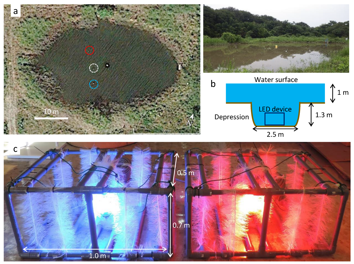
2.1. Experimental Pond

The study was conducted in a riverside aquatic experimental area of the Aqua Restoration Research Center, Public Works Research Institute, in Kakamigahara City, Gifu Prefecture, Japan. There were several flat-bottom elliptical ponds (length: 50 m, width: 30 m) that were filled with river water (approximately 1 m deep and 560 m³ volume) for experimental purposes. In these ponds, algal blooms were often observed in summer. In one of the ponds, three circular depressions (diameter: 2.5 m, depth: 1.3 m) with 3–4 m spacing were created, and a device (either a blue or red LED treatment or control) was installed in each depression (Figure 1a,b).

2.2. LED Devices

LED light sources in the blue (400–500 nm) and red (600–700 nm) wavelength ranges were used to illuminate the bottom of the depressions. The red (LW-50R1, 50-W) or blue (LW-100B1, 100-W) LED lights (Takuyo Riken Co., LTD., Fukuoka, Japan) were housed in a cylindrical waterproof case (diameter: 0.07 m, height: 0.2 m, water pressure resistance), and were hung in the center of a rectangular frame (PVC pipe, length: 1 m, width: 0.5 m, height: 0.7 m) to provide 360° of illumination in the horizontal direction (Figure 1c). Polypropylene filaments were also arranged inside the frame as a substrate for the attachment and proliferation of periphyton. A frame without light was used for the control. The devices were carefully placed in the depressions (arranged with the control in the middle and the blue and red LEDs at the sides, Figure 1a), and the LED lights were maintained to run continuously over the entire experiment.

2.3. Experimental Period and Measurements

The experiment commenced at the end of August 2015 and continued up until the following February. After filling the pond with river water at the beginning, there was no additional inflow during the experiment except for rainfall. Water temperature, dissolved oxygen (DO), pH, electrical conductivity (EC), and turbidity were monitored using a multiparameter water quality logger (W-22XD, Horiba, Ltd., Kyoto, Japan). Light quantum under the water was measured using a logger (DEFI-L, JAE Advantech Co., Ltd., Nishinomiya, Japan). The water quality sensors were set 0.2 m above the bottom of each depression via attachment to a vertically standing steel pipe. The sensors for light were located 1.0 m above the bottom, and facing upwards, to detect the availability of natural light (i.e., solar radiation) in these depressions. Data were recorded at 1 h intervals over the entire experimental period. Additionally, rainfall and air temperature data were collected during the survey from the nearest monitoring station (Gifu, 5 km northwest of the experimental site) of the Automated Meteorological Data Acquisition System (AMeDAS).

Water samples (500 mL) were collected 0.1 m above the sediment in each of the depressions using a hand pump tube (inside diameter: 5 mm) at the end of the experiment. These samples were analyzed for total nitrogen (TN) and total phosphorus (TP) using a continuous flow analysis auto-analyzer (swAAt, BL TEC K.K., Osaka, Japan), and for ammonium nitrogen (NH₄–N), nitrate nitrogen (NO₃–N), and phosphate phosphorus (PO₄–P), using an ion chromatography system (DIONEX DX-120) and a portable colorimeter (Orion AQ3700) (Thermo Fisher Scientific K.K., Tokyo, Japan).

A 15 mL of each bottom water sample was fixed using 2% formalin and used to analyze phytoplankton and zooplankton composition. The substrate filaments near the LED lights were also sampled at 5 cm, to analyze the periphytic algae and zoobenthos, at the end of the experiment. The filaments were placed in 15 mL centrifuge tubes, so as not to disturb the filament surfaces during cutting using scissors. The samples were also fixed by 2% formalin. These plankton and periphyton samples were then centrifuged at 3000 rpm for 30 min, and 10- to 15-fold concentrated solutes were extracted. To evaluate the phytoplankton and zooplankton compositions, a total of 1 mL of each sample was transferred multiple times to plankton counting chambers (MCP-200, Matsunami Glass Ind., Ltd., Osaka, Japan), and the phytoplankton and zooplankton were visually identified and manually enumerated at 40 to 300× magnification under an OLYMPUS BX50 phase contrast microscope (Olympus Corporation, Tokyo, Japan).

2.4. Statistical Analysis

Because it may take time for the water quality to acclimate to the created depressions, the whole experimental period was divided into several sub-periods according to the changing patterns of water quality and the rainfall occurrence, as in the Result section. Differences in water quality between the control and the treatments were tested using analysis of variance (ANOVA) for each period. Two-way ANOVA without repetition was performed for the daily mean and diel change (maximum to minimum difference) for DO, pH, EC, and temperature, with the treatment (control, red LED, and blue LED) and day (38–48 days each period) as the factors. If the effect of the treatment was significant, Dunnett’s test (priori comparison), which compares the control and each of the two treatments, was performed. For all tests, an α-value of 0.05 was used to determine the significance of the effects. All statistical tests were performed using R software (version 4.0.3; R Development Core Team, Vienna, Austria) with the package “multcomp”.

3. Results

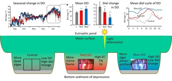
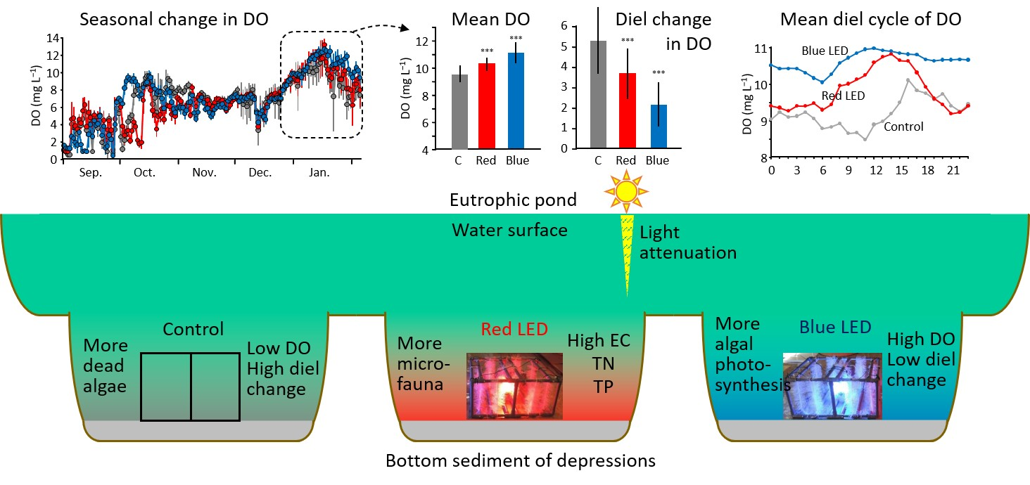
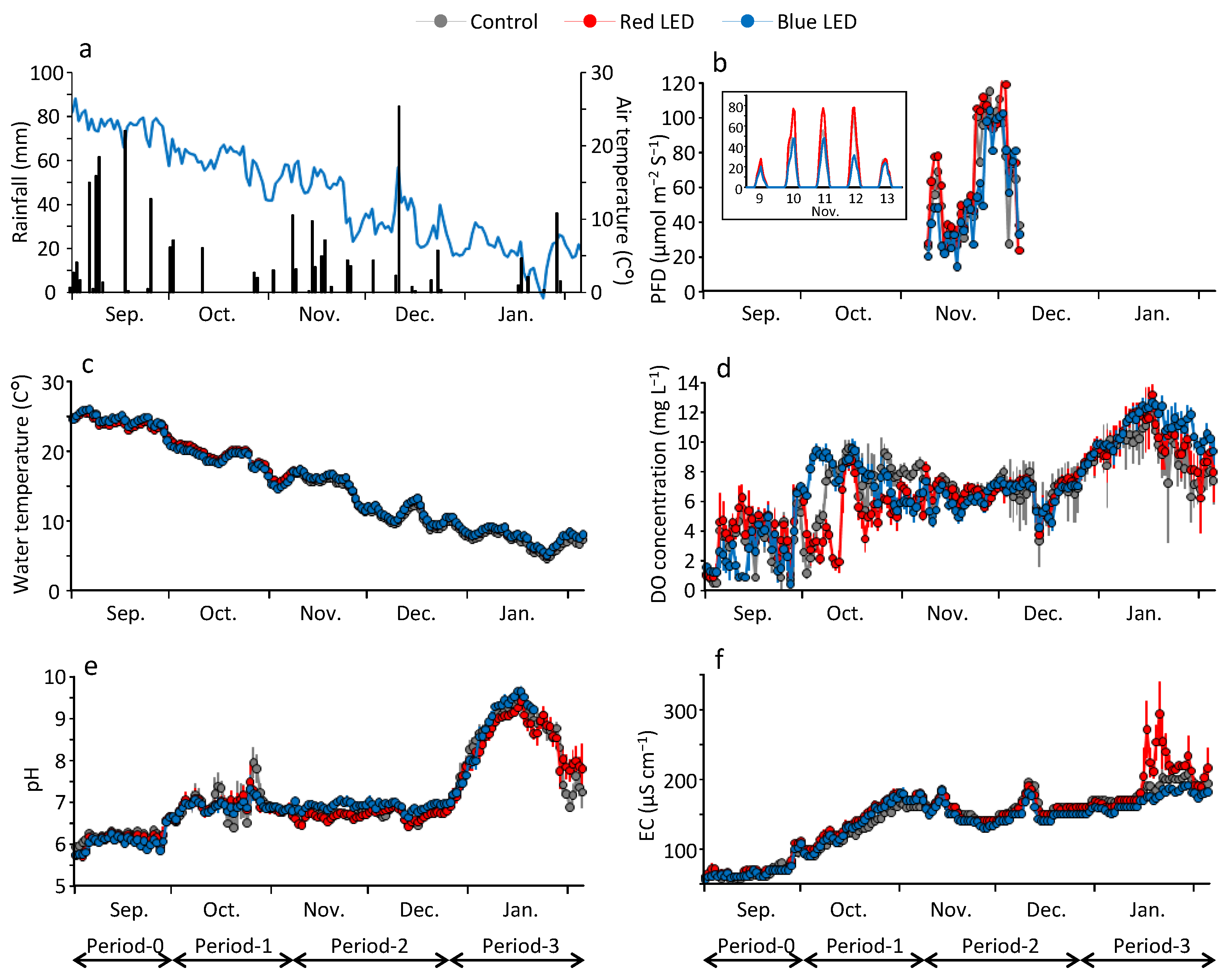
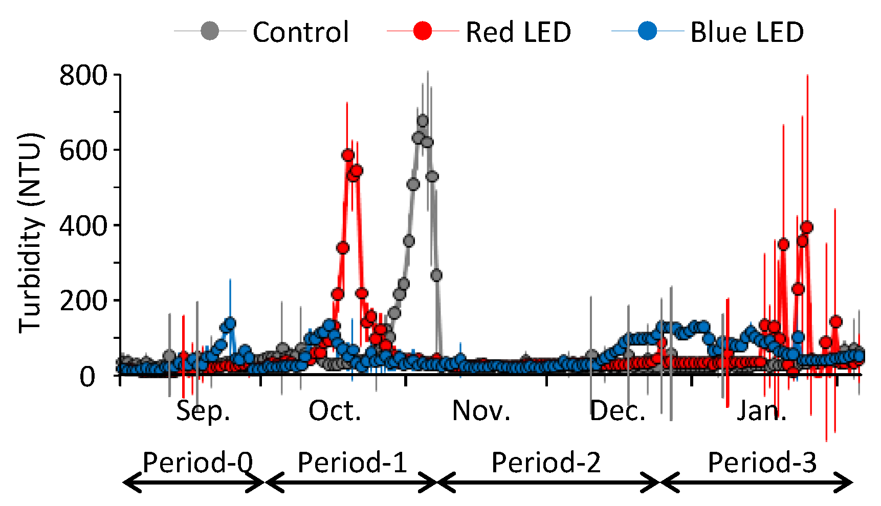
3.1. Overall Changes in Water Quality of the Pond during the Experiment

Rainfall occurred frequently in September and November, and less frequently in October and January, with a maximum rainfall (84.5 mm) in December (Figure 2a). The mean air temperature changed from 31.1 °C in early September to −5.0 °C in late January during the experiment.

The solar radiation that penetrated the water was captured by the light quantum sensor facing upward in the depressions for one month from November to December (Figure 2b). Although we expected a limited light availability in the depressions, the photon flux density sometimes exceeded 100 μmol m⁻² s⁻¹. Its diel cycle was obvious, with zero photons at night and a peak density at around noon every day (as shown in the small frame of Figure 2b). No photons at night indicated that the sensor captured the solar radiation but not the light from the LED. The depression of the control and red LED tended to have a higher photon flux density than that of the blue LED.

The water temperature changed from a range of 25 to 26 °C in early September to 4 to 5 °C in late January (Figure 2c). The temperature gradually decreased during the experiment, while it often showed a minor increase after rainfall. The DO concentration fluctuated between <1 mg L⁻¹ and >4 mg L⁻¹ in all of the depressions in September, increased to 8–10 mg L⁻¹ in the first half of October, and became much more stable in November and afterward (Figure 2d). The DO constantly increased from the middle of December and peaked in the middle of January. Large error bars in the control and red LED treatments indicated that the diel change was large in these depressions. The pH was approximately 6 in all depressions in September, increasing to approximately 7 in early October, and it further increased from late December to 9–10 in the middle of January (Figure 2e). The EC was 60–70 μS cm⁻¹ in September, and it gradually increased and reached 160–180 μS cm⁻¹ by the end of October, and it was relatively stable afterward, except for the red LED, with temporal rises in January (Figure 2f). The EC sometimes increased slightly after a rainfall (e.g., after the rainfall on 11 December, Figure 2a,f). The turbidity substantially increased (>600 NTU) in the middle of October (red LED) and the beginning of November (control) (Figure A1 in Appendix A) when rainfall was none or less. An increase in the base level (>100 NTU, blue LED) and large fluctuation (0–900 NTU, red LED) were observed in the latter months.

According to the low and fluctuating DO and a constantly low pH and EC, it appeared that the water quality was at a pre-acclimation state inside the depressions in September. The change in EC suggested that the water quality of the depression reached a new equilibrium by the beginning of November. The DO and pH increased constantly from December and peaked in January, corresponding to less rainfall occurring during these periods. Accordingly, the entire experimental period was divided into a pre-acclimation period (from 1 to 30 September), an acclimation period (from 1 October to 7 November), and after the new equilibrium, a rainy period (From 8 November to 24 December), and a stable period (from 25 December to 5 February). The latter three periods (hereafter referred to as period-1, -2, -3, see also Figure 2) were used to compare the water quality of the depressions.

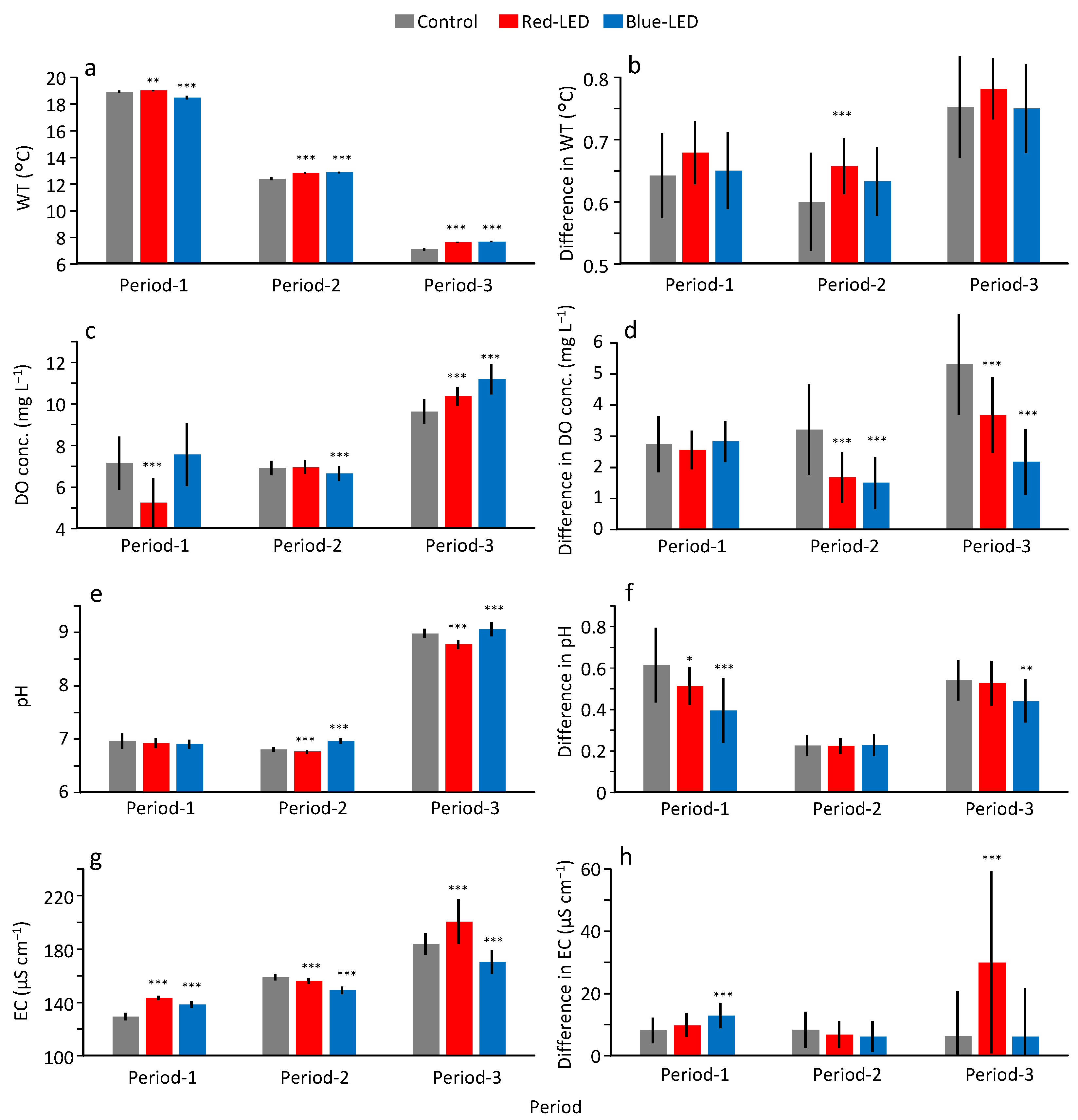
3.2. Differences in Water Quality of the Depressions in the Different Periods

Water temperature was significantly higher in the red and blue LED treatments than in the control in all periods except for the blue LED in period-1 (acclimation period) (Figure 3a). The temperature was 0.4–0.7 °C higher in the two LED treatments than in the control in period-2 (rainy period) and period-3 (stable period). The diel change (maximum to minimum difference) in temperature was 0.6–0.8 °C, and it tended to be slightly higher in the red LED than in the control (Figure 3b).

The DO concentration was significantly lower in the red LED than in the control in period-1, slightly but significantly lower in the blue LED than in the control in period-2, and significantly higher in the red and blue LED than in the control in period-3 (Figure 3c). In period-3, the DO was 0.7 mg L⁻¹ and 1.5 mg L⁻¹ higher in the red and blue LEDs, respectively, than in the control. The diel change in DO was significantly lower in the red and blue LEDs than in the control in period-2 and period-3 (Figure 3d). The mean diel change in DO in period-2 and period-3 was 3.2 mg L⁻¹ and 5.3 mg L⁻¹ in the control, and 1.5 mg L⁻¹ and 2.2 mg L⁻¹ in the blue LED, respectively.

The pH was significantly lower in the red LED than in the control in period-2 and period-3, while it was significantly higher in the blue LED than in the control in these periods (Figure 3e). The diel change in pH was significantly lower in the blue LED than in the control in period-1 and period-3, but it was similar between the control and the two LED treatments in period-2 (Figure 3f).

The EC was significantly higher in the red and blue LED than in the control in the period-1, while it was significantly lower in the blue LED than in the control in period-2 and period-3, and significantly higher in the red LED than in the control in the period-3 (Figure 3g). The diel change in EC was significantly higher in the blue LED than in the control in period-1, while it was significantly higher in the red LED than in the control in period-3 (Figure 3h).

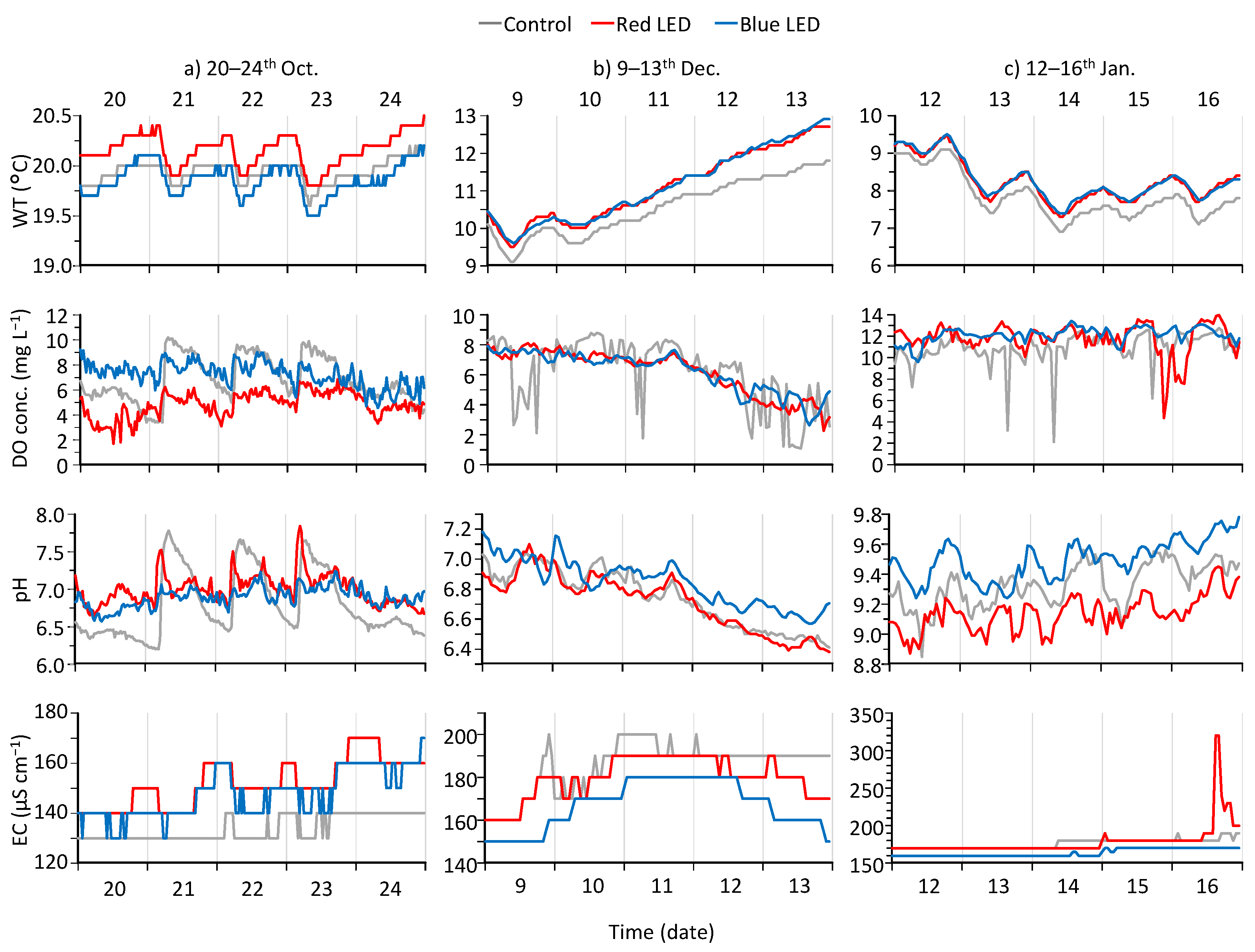
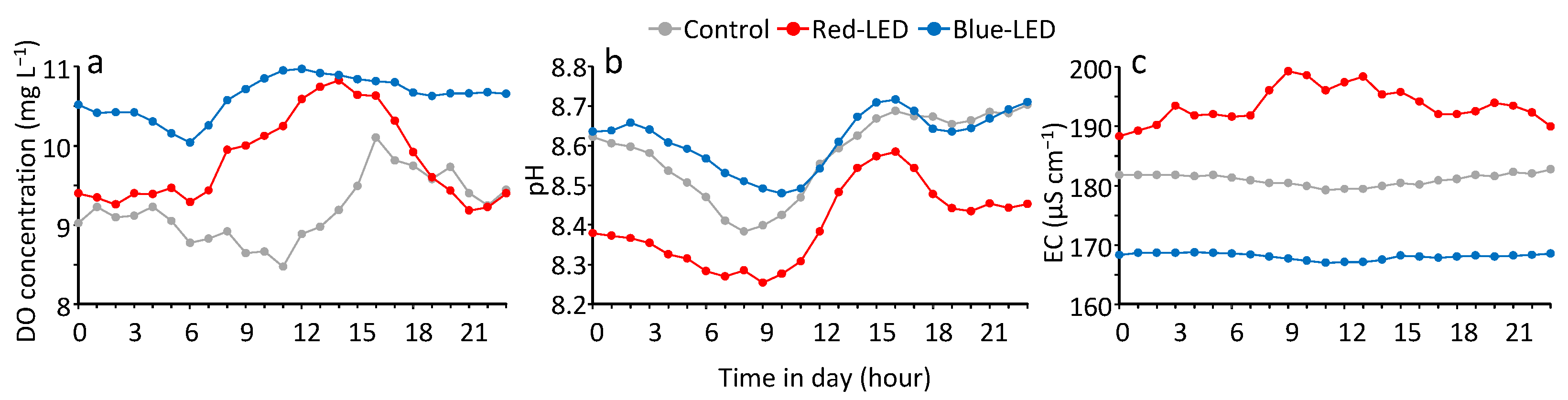
3.3. The Diel Cycle of Water Quality and the Response to Rainfall

A typical diel change in the water quality of the depressions in each period is shown in Figure 4. The first example is from 20 to 24 October without rainfall during these days and the preceding nine days (Figure 4a). The water temperature increased from morning to midnight and suddenly dropped at dawn. Inversely, the DO concentration decreased from morning to midnight, and then it suddenly rose at dawn, most conspicuously in the control. The change in pH was similar to that of DO in the control, while it was much more irregular in the blue LED. EC in the red LED treatment tended to increase at midnight. The water temperature increased and DO decreased continuously at dawn on the 24th when the diel change in air temperature was relatively low.

The second example is from 9 to 13 December, with rainfall on the second (7.5 mm) and third (84.5 mm) days (Figure 4b). The water temperature decreased from midnight to morning, and it increased in the afternoon on the first and second days, while it continuously increased from the third day. The difference in water temperature between the control and the two treatments gradually increased after rainfall. The DO concentration began to decrease from the afternoon of the third day. There was no apparent diel cycle in DO, while the fluctuation was large in the control. The pH also started decreasing from the afternoon of the third day, and it did not show a clear diel cycle. The EC tended to be high on the third day in all depressions.

The third example is from 12 to 16 January without rainfall during these days, nor over the preceding 19 days (Figure 4c). There was a clear diel cycle in the water temperature, with a minimum before noon and a maximum at midnight. Meanwhile, there was no clear diel cycle in the DO. The DO sometimes abruptly decreased by >3 mg L⁻¹ in the control and the red LED, with greater frequency and extent in the former. The pH tended to increase in the afternoon and decrease from midnight to morning, especially in the control and the blue LED. The EC was relatively stable over these days, except for the red LED, where the EC increased abruptly on the afternoon of the fifth day.

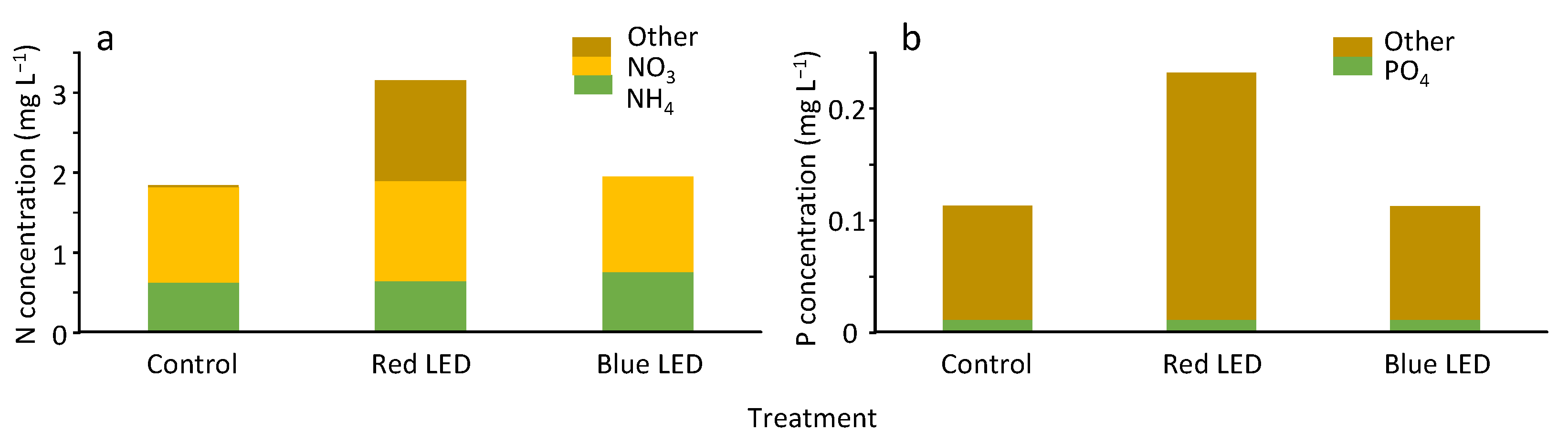
3.4. Nutrient Concentrations in the Depressions at the End of the Experiment

At the end of the experiment, the concentration of TN was higher in the red LED (3.15 mg L⁻¹) than in the control (1.85 mg L⁻¹) and the blue LED (1.95 mg L⁻¹) (Figure 5a). The concentrations of NH₄–N (0.63–0.76 mg L⁻¹) and NO₃–N (1.19–1.25 mg L⁻¹) were similar among the three depressions, while the concentration of the other fraction in TN, presumably organic-N, was higher in the red LED than in the others.

The concentration of TP was also higher in the red LED (0.23 mg L⁻¹) than in the control (0.11 mg L⁻¹) and blue LED (0.11 mg L⁻¹) (Figure 5b). The concentration of PO₄-P was similar among the three depressions (1.19–1.25 mg L⁻¹), while the concentration of the other fraction in TP, presumably organic-P, was twofold higher in the red LED (0.22 mg L⁻¹) than in the others (0.11 mg L⁻¹).

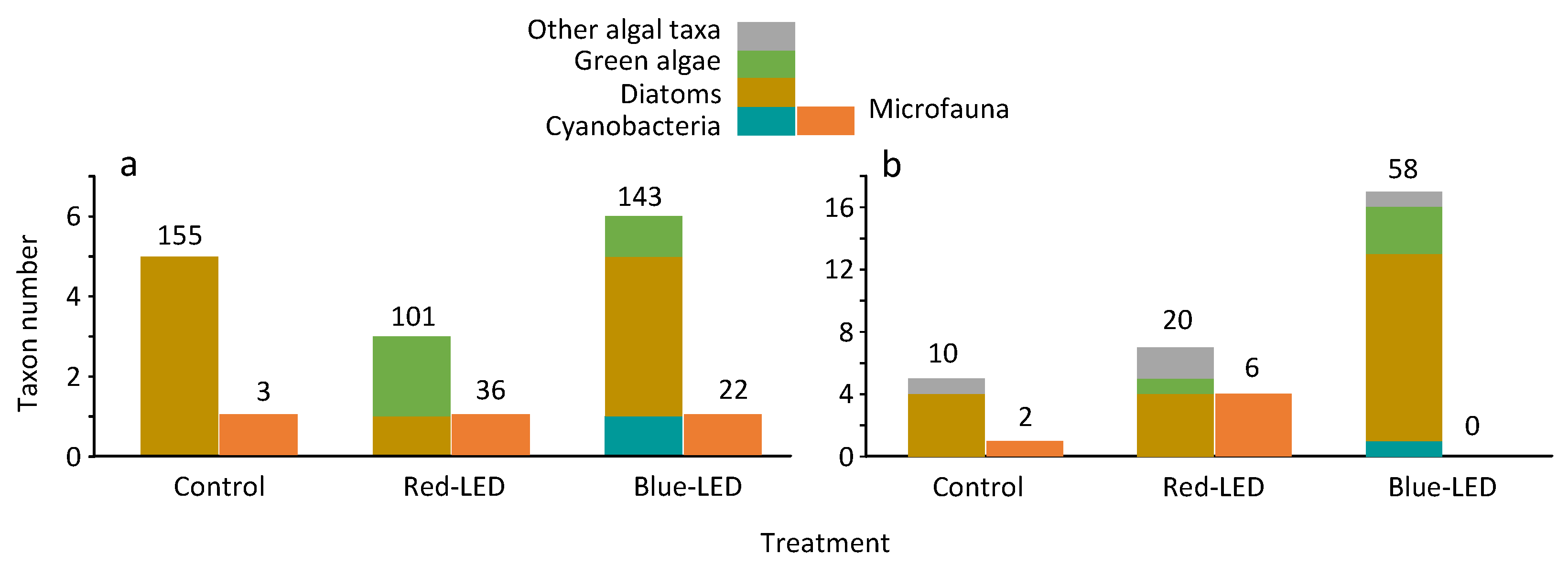
3.5. Periphyton and Phytoplankton Communities in the Depression at the End of the Experiment

In total, nine taxa (one cyanobacterium, six diatoms, and two green algae) occurred in the periphyton community on the filament of the device (Figure 6a,

Table A1. Cell abundance (cells mm⁻²) of algal and microfauna on the filament of device in the three depressions at the end of experiment.

Group	Taxa	Control	Red-LED	Blue-LED
Cyanobacteria	Phormidium			7
Bacillariophyta	Achnanthes	33		34
	Cocconeis	28	79	85
	Diatoma	16		2
	Gomphonema	49
	Melosira varians			1
	Rhoicosphenia	14
	Other taxa	15	12	13
Chlorophyta	Cladophora		1
	Oedogonium		9	1
Protozoa	Vorticella	3	36	22

). Only diatoms occurred in the control, while diatoms and green algae occurred in the red LED, and these algae and cyanobacteria occurred in the blue LED. The total algal cell abundance (cells mm⁻²) was lower in the red LED than in the others. Although diatoms, including Gomphonema and Achnanthes, were dominant in the control, many of them had ruptured/dead cells. Meanwhile, Cocconeis was the dominant taxon in the red and blue LED. In the red LED depression, filamentous green algae Cladophora and Oedogonium occurred. Due to their volume (more than 200–300-fold of the volume of many diatoms), algal abundance was higher in the red LED than in the control in terms of algal volume. As a microfauna (zoobenthos), the protozoa Vorticella occurred in all of the depressions, with a 12-fold higher abundance in the red LED than in the control.

In total, 21 taxa (1 cyanobacterium, 15 diatoms, 3 green algae, and 2 other algae) occurred in the plankton community in the three depressions (Figure 6b,

Table A2. Cell abundance (cells 0.1 mL⁻¹) of phytoplankton and zooplankton in water in the three depressions at the end of experiment.

Group	Taxa	Control	Red-LED	Blue-LED
Cyanobacteria	Merismopedia			7
Bacillariophyta	Asterionella formosa			3
	Aulacoseira distans			2
	Achnanthes			2
	Cyclotella	1	11	3
	Cymbella			2
	Diatoma		1
	Gomphonema acuminatum		1
	Melosira varians	3	1	1
	Navicula			3
	Nitzschia acicularis	1		7
	Nitzschia palea			1
	Nitzschia			2
	Synedra acus			1
	Synedra ulna			4
	Other taxa	1
Chlorophyta	Chlorella			1
	Oocystis			3
	Scenedesmus		4	8
Other algae	Cryptomonas		1
	Dinoflagellate	4	1	8
Protozoa	Amoeba		1
	Ciliata	2
	Tintinnopsis		1
Rotifer	Keratella		1
Crustacea	Nauplius		3

). Only diatoms and Dinoflagellate occurred in the control, while diatoms, green algae, and other algae (Cryptomonas, Dinoflagellate) occurred in the red LED, and these algae and cyanobacterium occurred in the blue LED. The total algal cell abundance (cells mL⁻¹) was the highest in the blue LED and the lowest in the control. The diatom Cyclotella was the most dominant taxon, followed by the green alga Scenedesmus in the red LED and the cyanobacterium Merismopedia, the diatom Nitzschia acicularis, the green alga Scenedesmus, and dinoflagellates were more abundant in the blue LED. More zooplankton taxa occurred in the red LED (four taxa) than in the control (one taxa) and the blue LED (none). The total cell abundance of zooplankton was also greater in the red LED than in the control.

4. Discussion

This study examined the effects of LED illumination on bottom water quality in a field experimental pond via the monitoring of DO, pH, EC, and temperature for 5 months. Although the differences in DO were minor or unclear among the depressions in the acclimation period and rainy period, the daily mean DO was significantly higher, and the diel change in DO was significantly lower in the blue LED than in the control in the stable period, one month after the water quality reached a new equilibrium. The differences in pH and EC between the control and blue LED were also clear. The effects of the red LED on DO were also detected, but to a lesser extent compared to those of the blue LED. Meanwhile, unexpectedly higher EC and nutrient concentrations were observed in the red LED. More periphyton and phytoplankton taxa occurred in the blue LED treatment than in the control, while more zoobenthos and zooplankton occurred in the red LED than in the control. The internal and external factors that have possibly affected the responses of water in the depressions to the LED treatments and the differences in effects between the red and blue LEDs are discussed in the following sections.

4.1. Differences in LED Effects among the Experimental Periods

The water quality in the depressions seemed not to have acclimated in the early periods of the experiment. The DO was lower than 6 mg L⁻¹, and the pH was less than 6.5 in September (period-0: pre-acclimation period). This was probably due to the frequent rainfall and the turbid water generated from the installation of the devices, which inhibited algal photosynthetic activity in the pond. The DO increased to 6–10 mg L⁻¹ and the pH increased to around 7 in October (period-1: acclimation period) when rainfall occurred less frequently. Meanwhile, the EC changed from <70 μS cm⁻¹ at the end of September to >160 μS cm⁻¹ at the end of October. The increase in EC was assumed to be associated with an exchange of water between the pond and the soil, and with an increase in solutes from the soil after the filling of ponds with river water at the end of August. These changes suggest that it took more than 2 months for the water quality of the depressions to reach a new equilibrium after the creation of the depressions.

The night cooling of the water surface of the pond by air was assumed to have induced a vertical mixing of water that temporally increased the DO in the depressions in period-1 (the acclimation period). Diel cycles in water temperature, DO, and pH were evident when there was no rainfall for several days in October (Figure 4a). The increases in DO and pH were conspicuous, and they corresponded to a decrease in water temperature at midnight, especially in the control. The surface water with a higher DO was considered to go downward as it became cooler and heavier in the nighttime. Such a diel circulation cycle with a vertical stratification in daytime and destratification in nighttime has been reported in shallow ponds [39,40], and such a polymictic nature may be a characteristic of small ponds with less thermal capacity. The effect of the LED on DO is difficult to detect in such circulating conditions. Meanwhile, the diel cycle of DO was small in January (period-3: stable period) even without rainfall for several days, probably because of the overall lower and smaller vertical difference in the water temperature.

Algal photosynthesis was likely to be the major process of increasing DO in the pond. Although oxygen from the atmosphere readily enters the surface, the oxygen diffuses slowly into the deeper layer in still water without a mixing process [41]. In addition, the oxygen transfer rate from the air to water is relatively high only when the DO concentration is far below the 100% saturation level. In the case of October (Figure 4a), DO varied from 5.0 to nearly 10 mg L⁻¹ in the control depression, and DO concentration at the surface layer of the pond was supposed to be higher than this. Because the DO concentration with 100% saturation is about 8.8 mg L⁻¹ under 20 °C, the rapid increase in DO below 100% saturation and any increases of DO in supersaturation level at the surface layer can be promoted only by photosynthesis. Meanwhile, the decrease of DO from morning to midnight in the depression may represent oxygen consumption by heterotrophic microbes. Further studies with coupled biological-hydrological model are needed to eludidate the contribution of different processes on the DO dynamics in ponds including diffusion from atmosphere, photosynthesis, and consumption by microbes [42].

DO tended to decrease after rainfall. DO and pH decreased in all of the depressions after a rainfall in December (Figure 4b), which was the largest rainfall during the experiment (Figure 2a). There was also a gradual increase in EC corresponding to the rainfall (Figure 4b). Because there was no apparent drain from the surrounding area, saturated water in the soil with a lower DO and a higher EC appeared to have inflowed into the pond after the rain. The water temperature often increased after the rainfall, and to a much greater extent in the red and blue LED than in the control. Being located near the periphery of the pond, the depressions in the red and blue LED treatments may have been more greatly affected by the water from the soil compared to that of the control. The frequent occurrence of rainfall in period-2 (rainy period) was likely to have obscured the effects of LED on DO.

The effects of LED on DO were evident in period-3, when there was less rainfall. In this period, DO and pH increased constantly from late December and reached a peak in the middle of January (Figure 2d,f), for instance, the daily mean DO in the control increased from 7.0 mg L⁻¹ (61% saturation) to 11.8 mg L⁻¹ (98%). Although such increases in DO and pH were likely to be associated with the photosynthetic activities of algae, because all of the depressions showed similar changes, the major light source for the photosynthesis was assumed to be solar radiation, rather than LED. The solar radiation in the three depressions sometimes exceeded 100 μmol m⁻² s⁻¹, which is greater than the irradiation of the compensation points for many algal species [43]. Thus, algal photosynthesis was potentially possible in the daytime on sunny days in the depressions without LED illumination, and much more possible in the shallower areas of the pond.

The effects of the LED lights were evident on the base level and diel change of DO. On average, the DO was 1 and 2 mg L⁻¹ higher in the red and blue LEDs, respectively, than in the control in period-3 (Figure 3c). Moreover, the diel change in DO was considerably smaller with the blue LED (1 mg L⁻¹) than in the control (5 mg L⁻¹) (Figure 3d). A sudden decrease in DO often occurred in the control in December and January, as shown by the high standard deviation in Figure 2d, as well as in Figure 4b,c. Such a temporal decrease, but with less frequency and extent, was also evident in the red LED. Notably, such a temporal decrease tended to occur at a certain time of day (i.e., control: daytime, red LED: nighttime, Figure 4b,c), rather than randomly. Abrupt changes in DO have been shown in previous studies in shallow aquatic systems [39,40,44], and they may indicate the presence of different DO level layers, which change in vertical distribution according to a diel photosynthetic rhythm. A diel cycle of DO in period-3 based on the mean value of each hour in the day (Figure 7a) shows that the DO tended to be lowest in the morning and highest in the evening in the control, while the DO increased from the morning and peaked at noon to early afternoon in the red and blue LEDs. It appears that the DO remained high throughout the night in the blue LED, while the DO decreased during the night in the control and red LED and remained low in the morning in the control. Although the diel cycle for pH was similar among the depressions, a steep decrease tended to occur in the early morning for the control, and in the evening for the red LED (Figure 7b). The possible reasons for the difference in the diel cycle between the control and LED treatments will be further discussed in the next section.

The effects of the LED lights on limiting the release of nutrients from the sediment to the overlying water were not evident in this study. Nutrients, especially phosphate and ammonium, are easily released from the bottom sediment in the absence of oxygen [16,17]. Thus, the release of nutrients was most likely to occur in the control depression with the lowest DO concentration. However, the increases in nutrients were not observed in the control at the end of the experiment (Figure 5a,b), possibly because hypoxia (<2–3 mg DO L⁻¹) rarely occurred during period-3. To conclude the effects of LED on the nutrient release through increasing DO via algal photosynthesis, further experiments especially in summer time are needed.

4.2. Possible Algal and Microfaunal Activities in the Three Depressions

Algal activities were promoted most highly in the depression in the blue LED, according to the greatest number of algal taxa (including cyanobacteria, diatoms, and green algae) on the filament, and in the water, and the greatest cell abundance in the water. Although the greatest cell abundance on the filament was in the control, many of the algal cells were ruptured/empty. Thus, because of the attenuation of sunlight in the water, the light was not always sufficient near the bottom of the depression without LED light, which caused death to the previously colonized algae. In contrast, the algae in the red and blue LEDs appeared active; this included Cocconeis, which formed multiple layers on the filaments, and filamentous green algae (Cladophora and Oedogonium), which protruded such layers. Periphyton can develop, and algal activity can be greater on the sediment surface, which is more stable, than on the filament of the device. Thus, LED illumination can stimulate the growth of algae, which have been in a dormant stage on the sediment [45,46], and which subsequently constituted periphyton and phytoplankton communities.

The differences in DO among the depressions in period-3 were likely to have been associated with algal photosynthetic activities. In period-3, although DO was basically high in all of the depressions, an abrupt temporal decrease in DO occurred in the control and in the red LED, and with greater frequency and extent in the former. Furthermore, the temporal decrease in DO tended to occur in the daytime and in the nighttime for the control and the red LED, respectively. Steep decreasing trends of DO and pH in the evening in the red LED (Figure 7a,b) suggest that the photosynthetic activity was low at night, without sunlight. Meanwhile, the lowest DO and a steep decreasing trend of pH in the morning in the control (Figure 7a,b) suggest here that the photosynthetic activities were the lowest in the morning. It appears that algal photosynthetic activity in the control was limited until the photon density became sufficient around noon, due to a poor abundance of algae. It is assumed that the algal photosynthesis, stimulated by LED illumination, was kept active for the whole day in the blue LED, which stabilized the high DO levels by dampening the diel rhythms of photosynthesis and respiration that are associated with solar radiation in the pond.

The greater abundance of zoobenthos and zooplankton might have reduced algal abundance and photosynthetic activity in the red LED. The growth of algae, especially those of diatoms and green algae, may be more highly stimulated by blue than red wavelengths [36,37]. However, the low abundance of algae and the high abundance of microfauna in the red LED in both the periphyton and phytoplankton communities (Figure 6a,b) was unexpected. It appears that the algal abundance was reduced by predation pressure from the microfauna. Stalked protozoa Vorticella, which collect and feed on organic particles, were most abundant in the periphytic community in the red LED (Table A1). A rotifer Keratella, which can exploit a wide range of food including algae, occurred in the plankton community in the red LED (Table A2). In addition, despite the absence in the plankton samples, a large zooplankton Daphnia was visually abundant in the 500 mL water sample in the red LED depression. The higher nutrient concentration (N and P) in the red LED, especially in forms other than the measured inorganic forms, presumably organic-N and organic-P (Figure 5a, b), may support the greater feeding activities of the microfauna with the red LED (i.e., excretion and the leaching of solutes from ruptured algal cells). Notably, EC in the red LED tended to increase abruptly in the daytime in period-3 (Figure 4c and Figure 7c), which may be associated with the diel cycle in the vertical distribution of zooplankton [47,48]. Zooplankton might have been attracted by the light of a red wavelength [49], or by edible algal species growing under the red LED.

5. Conclusions

The effects of LED illumination on bottom water quality were examined in a field experimental pond via the monitoring of water temperature, DO, pH, and EC in three depressions, with or without LED devices, over 5 months. The effects of the LED lights were unclear in the earlier periods because of irregular changes in the water quality that were associated with the acclimation of the water to a new status, the vertical mixing of water in the pond due to stratifications in water temperature, and external water inflow after rainfall. In the latter period with less rainfall, the DO gradually increased in all of the depressions due to algal photosynthesis stimulated by solar radiation. Nevertheless, increases in the mean daily DO and pH, decreases in the mean EC and decreases in diel changes in DO, pH, and EC were evident in the blue LED treatment. Increases in abundance and in the taxon richness of algae in the periphyton and phytoplankton communities were also evident at the end of the experiment. Meanwhile, the effect of the blue LED on nutrient concentration was not detected. The effects of the red LED treatment on DO and pH were evident to a lesser extent, as compared to those of the blue LED. The lower abundance of algal cells in the periphyton and phytoplankton communities, and the higher nutrient concentrations and EC in the red LED treatment may be associated with a higher abundance of microfauna. Our results confirmed the applicability of LED illumination in improving the bottom water quality, especially for increasing DO levels in outdoor ponds. Further studies are needed to clarify the spatial and temporal extents of these effects under internal water circulation and external water inflow over various seasons.

References

1. Huisman, J.; Codd, G.A.; Paerl, H.W.; Ibelings, B.W.; Verspagen, J.M.; Visser, P.M. Cyanobacterial blooms. Nat. Rev. Microbiol. 2018, 16, 471–483. [Google Scholar] [CrossRef] [PubMed]
2. Yan, X.; Xu, X.; Wang, M.; Wang, G.; Wu, S.; Li, Z.; Sun, H.; Shi, A.; Yang, Y. Climate warming and cyanobacteria blooms: Looks at their relationships from a new perspective. Water Res. 2017, 125, 449–457. [Google Scholar] [CrossRef] [PubMed]
3. Qin, B.; Paerl, H.W.; Brookes, J.D.; Liu, J.; Jeppesen, E.; Zhu, G.; Zhang, Y.; Xu, H.; Shi, K.; Deng, J. Why Lake Taihu continues to be plagued with cyanobacterial blooms through 10 years (2007–2017) efforts. Sci. Bull. 2019, 64, 354–356. [Google Scholar] [CrossRef] [Green Version]
4. Hoagland, P.A.D.M.; Anderson, D.M.; Kaoru, Y.; White, A.W. The economic effects of harmful algal blooms in the United States: Estimates, assessment issues, and information needs. Estuaries 2002, 25, 819–837. [Google Scholar] [CrossRef]
5. Heisler, J.; Glibert, P.M.; Burkholder, J.M.; Anderson, D.M.; Cochlan, W.; Dennison, W.C.; Dortch, Q.; Gobler, C.J.; Heil, C.A.; Humphries, E.; et al. Eutrophication and harmful algal blooms: A scientific consensus. Harmful Algae 2008, 8, 3–13. [Google Scholar] [CrossRef] [Green Version]
6. Paerl, H.W.; Huisman, J. Blooms like it hot. Science 2008, 320, 57–58. [Google Scholar] [CrossRef] [Green Version]
7. Paul, V.J. Global warming and cyanobacterial harmful algal blooms. In Cyanobacterial Harmful Algal Blooms: State of the Science and Research Needs; Hudnell, H.K., Ed.; Advances in Experimental Medicine and Biology; Springer: New York, NY, USA, 2008; Volume 619, pp. 239–257. [Google Scholar]
8. O’Neil, J.M.; Davis, T.W.; Burford, M.A.; Gobler, C.J. The rise of harmful cyanobacteria blooms: The potential roles of eutrophication and climate change. Harmful Algae 2012, 14, 313–334. [Google Scholar] [CrossRef]
9. Schelske, C.L.; Hodell, D.A. Using carbon isotopes of bulk sedimentary organic matter to reconstruct the history of nutrient loading and eutrophication in Lake Erie. Limnol. Oceanogr. 1995, 40, 918–929. [Google Scholar] [CrossRef]
10. Koelmans, A.A.; Van der Heijde, A.; Knijff, L.M.; Aalderink, R.H. Integrated modelling of eutrophication and organic contaminant fate & effects in aquatic ecosystems. A review. Water Res. 2001, 35, 3517–3536. [Google Scholar]
11. Anderson, N.J.; Bennion, H.; Lotter, A.F. Lake eutrophication and its implications for organic carbon sequestration in Europe. Glob. Chang. Biol. 2014, 20, 2741–2751. [Google Scholar] [CrossRef] [Green Version]
12. Gorham, E.; Boyce, F.M. Influence of lake surface area and depth upon thermal stratification and the depth of the summer thermocline. J. Great Lakes Res. 1989, 15, 233–245. [Google Scholar] [CrossRef]
13. Foley, B.; Jones, I.D.; Maberly, S.C.; Rippey, B. Long-term changes in oxygen depletion in a small temperate lake: Effects of climate change and eutrophication. Freshw. Biol. 2012, 57, 278–289. [Google Scholar] [CrossRef]
14. Howarth, R.; Chan, F.; Conley, D.J.; Garnier, J.; Doney, S.C.; Marino, R.; Billen, G. Coupled biogeochemical cycles: Eutrophication and hypoxia in temperate estuaries and coastal marine ecosystems. Front. Ecol. Environ. 2011, 9, 18–26. [Google Scholar] [CrossRef] [Green Version]
15. Wang, H.; Dai, M.; Liu, J.; Kao, S.J.; Zhang, C.; Cai, W.J.; Wang, G.; Qian, W.; Zhao, M.; Sun, Z. Eutrophication-driven hypoxia in the East China Sea off the Changjiang Estuary. Environ. Sci. Technol. 2016, 50, 2255–2263. [Google Scholar] [CrossRef]
16. Wetzel, R.G. The phosphorus cycle. In Limnology, 3rd ed.; Wetzel, R.G., Ed.; Academic Press: Cambridge, MA, USA, 2001; pp. 239–288. [Google Scholar]
17. Hupfer, M.; Lewandowski, J. Oxygen controls the phosphorus release from Lake Sediments—A long-lasting paradigm in limnology. Int. Rev. Hydrobiol. 2008, 93, 415–432. [Google Scholar] [CrossRef]
18. Meyer-Reil, L.A.; Köster, M. Eutrophication of marine waters: Effects on benthic microbial communities. Mar. Pollut. Bull. 2000, 41, 255–263. [Google Scholar] [CrossRef]
19. Kang, M.; Tian, Y.; Peng, S.; Wang, M. Effect of dissolved oxygen and nutrient levels on heavy metal contents and fractions in river surface sediments. Sci. Total Environ. 2019, 648, 861–870. [Google Scholar] [CrossRef]
20. Beutel, M.W.; Leonard, T.M.; Dent, S.R.; Moore, B.C. Effects of aerobic and anaerobic conditions on P, N, Fe, Mn, and Hg accumulation in waters overlaying profundal sediments of an oligo-mesotrophic lake. Water Res. 2008, 42, 1953–1962. [Google Scholar] [CrossRef]
21. Liem-Nguyen, V.; Skyllberg, U.; Björn, E. Thermodynamic modeling of the solubility and chemical speciation of mercury and methylmercury driven by organic thiols and micromolar sulfide concentrations in boreal wetland soils. Environ. Sci. Technol. 2017, 51, 3678–3686. [Google Scholar] [CrossRef]
22. Diaz, R.J. Overview of hypoxia around the world. J. Environ. Qual. 2001, 30, 275–281. [Google Scholar] [CrossRef]
23. Arend, K.K.; Beletsky, D.; DePinto, J.V.; Ludsin, S.A.; Roberts, J.J.; Rucinski, D.K.; Scavia, D.; Schwab, D.J.; Höök, T.O. Seasonal and interannual effects of hypoxia on fish habitat quality in central Lake Erie. Freshwat. Biol. 2011, 56, 366–383. [Google Scholar] [CrossRef] [Green Version]
24. Li, Y.; Wang, L.; Yan, Z.; Chao, C.; Yu, H.; Yu, D.; Liu, C. Effectiveness of dredging on internal phosphorus loading in a typical aquacultural lake. Sci. Total Environ. 2020, 744, 140883. [Google Scholar] [CrossRef] [PubMed]
25. Beutel, M.W.; Horne, A.J. A review of the effects of hypolimnetic oxygenation on lake and reservoir water quality. Lake Reserv. Manag. 1999, 15, 285–297. [Google Scholar] [CrossRef] [Green Version]
26. Bessa da Silva, M.; Gonçalves, F.; Pereira, R. Portuguese shallow eutrophic lakes: Evaluation under the Water Framework Directive and possible physicochemical restoration measures. Euro-Mediterr. J. Environ. Integr. 2019, 4, 3. [Google Scholar] [CrossRef]
27. Hao, A.; Kobayashi, S.; Xia, D.; Mi, Q.; Yan, N.; Su, M.; Lin, A.; Zhao, M.; Iseri, Y. Controlling eutrophication via surface aerators in irregular-shaped urban ponds. Water 2021, 13, 3360. [Google Scholar] [CrossRef]
28. Li, L.; Li, Y.; Biswas, D.K.; Nian, Y.; Jiang, G. Potential of constructed wetlands in treating the eutrophic water: Evidence from Taihu Lake of China. Bioresour. Technol. 2008, 99, 1656–1663. [Google Scholar] [CrossRef]
29. Zhao, F.; Xi, S.; Yang, X.; Yang, W.; Li, J.; Gu, B.; He, Z. Purifying eutrophic river waters with integrated floating island systems. Ecol. Eng. 2012, 40, 53–60. [Google Scholar] [CrossRef]
30. Waajen, G.W.; Van Bruggen, N.C.; Pires, L.M.D.; Lengkeek, W.; Lürling, M. Biomanipulation with quagga mussels (Dreissena rostriformis bugensis) to control harmful algal blooms in eutrophic urban ponds. Ecol. Eng. 2016, 90, 141–150. [Google Scholar] [CrossRef]
31. Keeling, P.J. The number, speed, and impact of plastid endosymbioses in eukaryotic evolution. Annu. Rev. Plant Biol. 2013, 64, 583–607. [Google Scholar] [CrossRef] [Green Version]
32. Carvalho, A.P.; Silva, S.O.; Baptista, J.M.; Malcata, F.X. Light requirements in microalgal photobioreactors: An overview of biophotonic aspects. Appl. Microbiol. Biotechnol. 2011, 89, 1275–1288. [Google Scholar] [CrossRef]
33. Blanken, W.; Cuaresma, M.; Wijffels, R.H.; Janssen, M. Cultivation of microalgae on artificial light comes at a cost. Algal Res. 2013, 2, 333–340. [Google Scholar] [CrossRef]
34. Schulze, P.S.; Barreira, L.A.; Pereira, H.G.; Perales, J.A.; Varela, J.C. Light emitting diodes (LEDs) applied to microalgal production. Trends Biotechnol. 2014, 32, 422–430. [Google Scholar] [CrossRef] [PubMed]
35. Olle, M.; Viršile, A. The effects of light-emitting diode lighting on greenhouse plant growth and quality. Agric. Food Sci. 2013, 22, 223–234. [Google Scholar] [CrossRef]
36. Kwon, H.K.; Oh, S.J.; Yang, H.S.; Kim, P.J. Phytoremediation by benthic microalgae (BMA) and light emitting diode (LED) in eutrophic coastal sediments. Ocean Sci. J. 2015, 50, 87–96. [Google Scholar] [CrossRef]
37. Hao, A.; Kobayashi, S.; Yan, N.; Xia, D.; Zhao, M.; Iseri, Y. Improvement of water quality using a circulation device equipped with oxidation carriers and light emitting diodes in eutrophic pond mesocosms. J. Environ. Chem. Eng. 2021, 9, 105075. [Google Scholar] [CrossRef]
38. Hao, A.; Yu, H.; Kobayashi, S.; Xia, D.; Zhao, M.; Iseri, Y. Effects of light-emitting diode illumination on sediment surface biological activities and releases of nutrients and metals to overlying water in eutrophic lake microcosms. Water 2022, 14, 1839. [Google Scholar] [CrossRef]
39. Chang, W.Y.; Ouyang, H. Dynamics of dissolved oxygen and vertical circulation in fish ponds. Aquaculture 1988, 74, 263–276. [Google Scholar] [CrossRef] [Green Version]
40. Andersen, M.R.; Kragh, T.; Sand-Jensen, K. Extreme diel dissolved oxygen and carbon cycles in shallow vegetated lakes. Proc. R. Soc. B Biol. Sci. 2017, 284, 20171427. [Google Scholar] [CrossRef]
41. Boyd, C.E. Pond water aeration systems. Aquac. Eng. 1988, 18, 9–40. [Google Scholar] [CrossRef]
42. Prokopkin, I.G.; Zadereev, E.S. A model study of the effect of weather forcing on the ecology of a meromictic Siberian lake. J. Oceanol. Limnol. 2018, 36, 2018–2032. [Google Scholar] [CrossRef]
43. Kirk, J.T.O. Photosynthesis as a function of the incident light. In Light and Photosynthesis in Aquatic Ecosystems, 3rd ed.; Kirk, J.T.O., Ed.; Cambridge University Press: Cambridge, UK, 2011; pp. 330–387. [Google Scholar]
44. Langman, O.C.; Hanson, P.C.; Carpenter, S.R.; Hu, Y.H. Control of dissolved oxygen in northern temperate lakes over scales ranging from minutes to days. Aquat. Biol. 2010, 9, 193–202. [Google Scholar] [CrossRef]
45. Sederias, J.; Colman, B. The interaction of light and low temperature on breaking the dormancy of Chara vulgaris oospores. Aquat. Bot. 2007, 87, 229–234. [Google Scholar] [CrossRef]
46. Zou, W.; Wang, Z.; Song, Q.; Tang, S.; Peng, Y. Recruitment-promoting of dormant Microcystis aeruginosa by three benthic bacterial species. Harmful Algae 2018, 77, 18–28. [Google Scholar] [CrossRef]
47. Hays, G.C. A review of the adaptive significance and ecosystem consequences of zooplankton diel vertical migrations. In Migrations and Dispersal of Marine Organisms; Developments in Hydrobiology; Jones, M.B., Ingólfsson, A., Ólafsson, E., Helgason, G.V., Gunnarsson, K., Svavarsson, J., Eds.; Springer: Dordrecht, The Netherland, 2003; Volume 174, pp. 163–170. [Google Scholar]
48. Williamson, C.E.; Fischer, J.M.; Bollens, S.M.; Overholt, E.P.; Breckenridge, J.K. Toward a more comprehensive theory of zooplankton diel vertical migration: Integrating ultraviolet radiation and water transparency into the biotic paradigm. Limnol. Oceanogr. 2011, 56, 1603–1623. [Google Scholar] [CrossRef] [Green Version]
49. Martynova, D.M.; Gordeeva, A.V. Light-dependent behavior of abundant zooplankton species in the White Sea. J. Plankton Res. 2010, 32, 441–456. [Google Scholar] [CrossRef] [Green Version]
Figure 1. Overview of the experimental pond and the location of three depressions (a), vertical view of the depressions (b), and LED devices (blue and red) (c).
Water 14 02310 g001
Figure 2. Changes in rainfall, mean air temperature (a), photon flux density (b), water temperature (c), DO concentration (d), pH (e), and EC (f) of the 3 depressions in ponds during the experiment. Daily maximum (with example diel cycle in a small frame) (b) and daily mean (±1SD) (cf) are shown.
Water 14 02310 g002
Figure 3. Differences in water quality of the depression between the control and LED treatments ((a): daily mean temperature, (b): diel temperature change, (c): daily mean DO, (d): diel DO change, (e): daily mean pH, (f): diel pH change, (g): daily mean EC, (h): diel EC change). Error bars are SD of the difference from the mean each day. Asterisks show the significance of the difference between the control and LED treatment (*: p < 0.05, **: p < 0.01, ***: p < 0.001).
Water 14 02310 g003
Figure 4. Hourly changes in water quality (water temperature, DO, pH, and EC) of the 3 depressions for 5 days ((a): 20–24 October, (b): 9–13 December, (c): 12–16 January).
Water 14 02310 g004
Figure 5. Nutrient concentrations ((a): nitrogen, (b): phosphorus) in the depressions at the end of the experiment. Other shows the fraction other than the measured inorganic forms in TN/TP.
Water 14 02310 g005
Figure 6. The number of taxa occurring in the periphyton community on the filament (a) and in the plankton community from the water (b) of the three depressions. The number on the bars shows the total cell abundance ((a): cells mm−2, (b): cells 0.1 mL−1).
Water 14 02310 g006
Figure 7. Diel change in DO (a), pH (b), and EC (c) based on the mean value of each hour in the day during period-3.
Water 14 02310 g007
Publisher’s Note: MDPI stays neutral with regard to jurisdictional claims in published maps and institutional affiliations.