
Simulating Dynamics and Ecology of the Sea Ice of the White Sea by the Coupled Ice–Ocean Numerical Model


1
Institute of Applied Math Research, Karelian Research Centre of RAS, 185035 Petrozavodsk, Russia
2
Northern Water Problems Institute, Karelian Research Centre of RAS, 185035 Petrozavodsk, Russia
3
Marchuk Institute of Numerical Mathematics of the RAS, 119333 Moscow, Russia
*
Author to whom correspondence should be addressed.
†
These authors contributed equally to this work.
Water 2022, 14(15), 2308; https://doi.org/10.3390/w14152308
Submission received: 2 June 2022
/
Revised: 15 July 2022
/
Accepted: 22 July 2022
/
Published: 25 July 2022
(This article belongs to the Special Issue Advances in Numerical Modelling of Sea Dynamics)
Abstract
:In this paper, a numerical model of the White Sea is presented. The White Sea is a small shallow sea with strong tidal currents and complex ice behavior. The model is the only comprehensive numerical model for the White Sea. It consists of several coupled submodels (for water, ice, pelagic, and sympagic ecology). In this work, the focus is on the dynamics of sea ice and its ecosystem. The model is described and its results are compared to available sea–ice data, mostly satellite data. The spatial resolution of the model is 3 km. High current velocities require the time step of 3 min. The model is shown to reproduce sea–ice concentration well; in particular, timing of the sea ice is perfect. The dynamics of the sea–ice ecosystem also looks reasonable. Chlorophyll-a content agrees well with measurements, and the ratio of algal, bacterial, and faunal biomass is correct. Sympagic biomass is underestimated. Light is limiting at the early stage of sympagic bloom, nutrient limitation is for the second half. We show that sympagic component influences the spring bloom (in terms of timing and height of the peaks) but has little effect on the dynamics during the warm period of the year.
1. Introduction
The White Sea plays an important role in the economy of the North-West of the Russian Federation: the routes of the White Sea-Baltic Canal and the Northern Sea Route intersect here; the flow of tourists visiting the sights, including UNESCO sites, is constantly increasing; various biological and mineral resources are also available. Therefore, information about the sea–ice regime is important for performing safe navigation during a long period of the year (from November to May). It is important to forecast timing and specifics of ice formation and ice breakup, and dangerous ice phenomena in river estuaries (for example, areas of jams, accumulations, presence of ice fields).
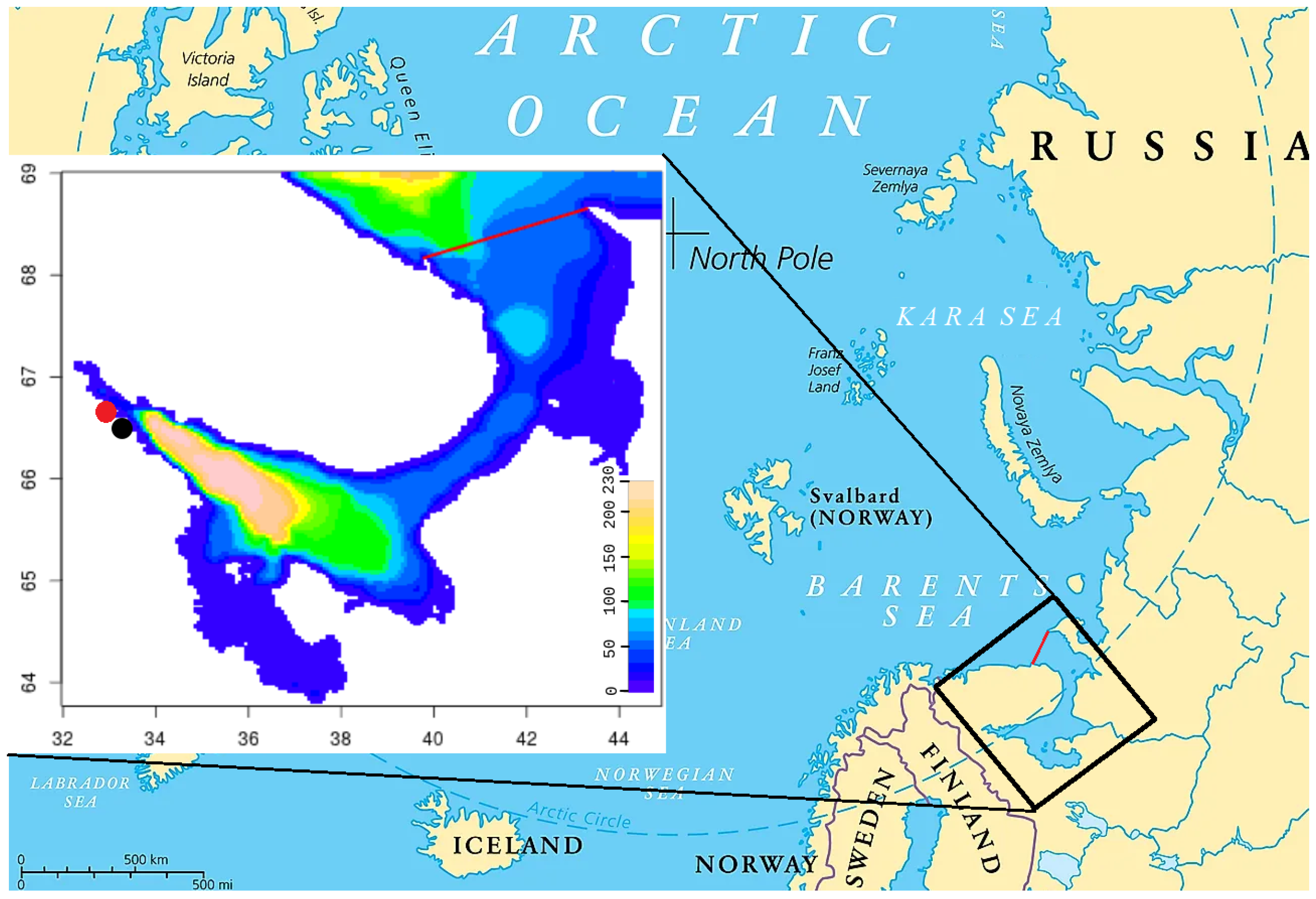
The White Sea is a small shallow sea in northwestern Russia. Its surface area is 91,000 km; its average depth is about 67 m, with a small deep area up to 340 m (Figure 1). The coastline has a length of more than 5 thousand km [1]. Different bays and parts of the White Sea differ significantly in their features. In particular, the sea is divided into two parts of comparable size (33% and 55% of the sea) separated by a shallow (37 m) and narrow (45–55 km) strait called the Gorlo. The sea has one liquid boundary with the Barents Sea. The incoming tidal wave creates a dominant pattern of tidal currents in the White Sea. Many rivers flow into the sea, so its salinity is lower than in the neighboring Barents Sea. These rivers also bring biogenic matter, which is important for the productivity of the sea. The balance between evaporation and precipitation is close to zero, so the monthly water exchange is shifted on average towards the outflow, which is very close to the monthly river discharge. However, on the daily scale the flow balance can be both in and out, due to the strong tide .
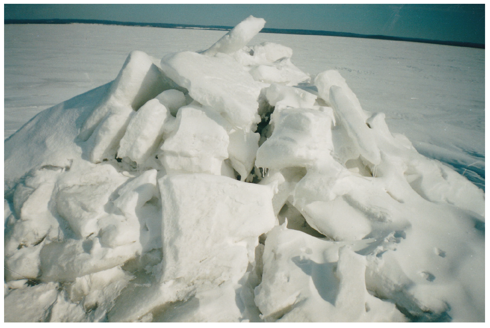
The White Sea is free of ice in the warm season. Although in winter the ice thickness is very heterogeneous and there are hummocks (a consequence of strong currents), there is no perennial ice in the sea. Due to significant daily variability in sea level, the ice often touches the bottom and becomes stratified, so it is heavier than normal ice. It may even contain surviving benthic organisms. Such a mechanism of capturing organic sediments from the bottom and releasing them far out into the water is typical for the White Sea. Run aground icebergs (grounded hummocks) are often found in the Sea near the coast; they are called “stamukha” (Figure 2) and melt later than other types of ice.
The collection of scientific data on sea ice off the coast of the White Sea was initiated in the late 19th century by the Lighthouse Service of the Maritime Ministry of Russia. Systematic observations of sea ice have been made since 1918 at coastal and island stations. Data on sea ice in the open sea were collected by ice-breakers and sea fishing vessels, the earliest data being from 1909. Since 1927, aerial reconnaissance data have been available for navigation. Initially, these data were collected with the beginning of the hunting season, i.e., in spring. Since 1948, this time was increased up to January–May, and later, in 1951, it covered the whole ice season of the White Sea. All these data until 1985 are analyzed in the works of the State Oceanographic Institute of the USSR [2]. This summary is very useful. However, due to climate change, ice phenomena on many lakes and seas have changed [3,4], so approaches need to change. A modern source of data on the ice cover of lakes and seas is satellite remote sensors [5,6]. Satellite data can provide much information about sea ice because of the high spatial and temporal resolution important for understanding sea–ice dynamics.
There is a large amount of satellite data on the sea–ice concentration in the White Sea; in particular, NASA (https://www.nasa.gov/, accessed on 2 June 2022) has collected a lot of data on various seas, including the White Sea, using the MODIS sensor with spatial resolution up to 250 m. The National Snow and Ice Center NSIDC (https://nsidc.org/, accessed on 2 June 2022) offers data with resolution 4–6 km. The NOAA NESDIS center lso provides their data with this resolution (https://www.nesdis.noaa.gov/, accessed on 2 June 2022). Additional resources are surveyed in our review [7]. However, numerical models are needed for ice forecasts, climatic scenarios, etc.
In situ data on sympagic ecological systems are needed to validate the models. However, due to the difficulties of winter expeditions in the White Sea, data are scarce. Most sea–ice samples were obtained at the White Sea biostations of Moscow State University and the Zoological Institute of the Russian Academy of Sciences; these stations are not far from each other, both in the same bay (Figure 1). Some data were collected at river mouths. These data are analyzed in [8,9]. The ecosystems of the White Sea are described in [9,10,11,12,13]. However, the stations cover only a small part of the Sea. Moreover, most of the samples are taken near the shore (at the fast ice).
The development of models of sea–ice dynamics and ecology could stimulate special research in expeditions, and this could both provide more data to improve and test models and broaden our understanding of phenomena occurring in sea ice.
Although there are many mature sea circulation models, very few of them have been adapted (or specifically developed) for the White Sea. In addition to the model presented in this article, there is a White Sea operational model (without ice dynamics) [14]. Ivan Neelov’s model [1] has not been used nor maintained for more than ten years. No new model of the White Sea has appeared since [1] review in 2005, except ours. The same is true for models of marine ecology.
A separate problem is describing sympagic ecology (or cryosystem). Ice is capable of trapping and accumulating large amounts of organic and inorganic substances, which are then transported with ice drift across the sea over long distances and beyond the sea. All of the remaining ice melts by summer; this matter returns to the water, creating a “seeding” effect. During the winter, the biomass of cryo-algae changes. The blooming period is short, because sufficient light and therefore long daylight hours and thin ice with little snow on it are necessary; under these conditions, the ice comes off quickly. As the authors of [15,16] report, a proper description of sea–ice algae phenology and the links with pelagic and benthic systems are necessary to better understand ecosystem responses to warming and reduced ice cover. The effects of climate change on marine ecology and especially on sea–ice algae have been described in detail in [17,18].
The typical process of the sea–ice life cycle is described in the Results and Discussion section and compared to the model results.
Sea and river ice and snow on it play a significant role in the transport of terrigenous matter from the watershed. For example, the Northern Dvina river takes m of river ice annually into the White Sea; this ice contains 945 tons of sediment carried into the Dvinsky Bay [19]. The river itself carries much more sediment (over 4 million tons per year) [20]. On the other hand, the substance trapped by the ice can be carried far away by drifting ice and affect the pelagic ecology after the ice melts not only in the White Sea but also in the Barents Sea [20]. According to this work, there is more substance in the upper part of the ice: it came in with the snow and is considered anthropogenic. In spring, the lower part of the ice is also often rich in organic matter due to diatom algae [9] blooms. However, the content of organic matter in sea ice varies in different parts of the sea. Away from the rivers, suspended sediment concentration and sympagic phytoplankton productivity are lower, while both are much higher at river mouths [21].
The goal of this work was to create a comprehensive numerical model (called “Jasmine”) of processes in the White Sea: currents, thermohaline dynamics, state of the sea ice, pelagic, and sympagic ecology. The progress, compared to our paper [22], is twofold: first, the spatial resolution of the model was increased ( grid points to , or 8 km to 3 km); second, the ecological processes in sea–ice were taken into account. The model of the Arctic ocean FEMAO [23] (which describes currents, temperature, salinity, and sea ice) and BFM [24] (including the sea–ice ecology module [25]) have been coupled together. The BFM model, with the sea–ice submodel included, has never been coupled with ocean circulation models to our knowledge. This complex was adjusted to the special conditions of the White Sea and tested on the little available data (mostly satellite). The focus is on sea ice concentration, which can be both calculated from the model and estimated from satellite data, and biogeochemical tracers in the sea ice. The main change in the sea–ice model relative to the Arctic ocean model (used also in [22]) was the value of the “ridging” parameter: it was obtained in a series of numerical experiments and a theoretical explanation to the obtained value that gives reasonable model results is given. The model results are shown to reflect sea–ice concentration reasonably well. The dynamics of sympagic ecology also appear reasonable.
2. The Numerical Models
2.1. Sea Circulation Model
The numerical model Jasmine [22], based on the Finite-Element Model of the Arctic Ocean (FEMAO) [23] (see also references therein), was used to study the dynamics of sea ice in the White Sea. This model is capable of modeling three-dimensional current velocity, spatial. and temporal variability of water temperature, salinity, and sea level. The sea–ice component is described in a separate section. The pelagic and sympagic ecology components are coupled with the hydrodynamic model and can simulate fluxes of matter between different functional types of plankton, dissolved and particulate matter, sediment, biologically active sea–ice layer, etc. As far as we know, there are no other hydrodynamical models of the White Sea with sea ice and marine ecology. The model equations are written in cylinder-over-sphere coordinates, where the x-axis points north, the y-axis points east, and the z-axis points down. The spatial steps are ′ and ′ and correspond to a step of km along the meridian and to km along the parallel. The vertical grid consists of 41 layers: 0 m, 1 m, 3 m, 5 m; then 29 layers, each 5 m; then 8 more layers of 10 m each, to describe the deep sea. Note that the deepest point in the model is underestimated: this is the drawback of all available bathymetry sets [7].
The time step was 3 min. It is the largest time step that the model can use without blowups due to numerical instability, and it was chosen by numerical experiments. Tidal motions are strong in the White Sea, and also in the model, so current speed reaches 2 m/s in some points. The Courant condition is a serious restriction in this case. We made a numerical experiment with the “closed White Sea”, with no liquid boundary and, so, no tidal currents: the model does not blow up for the step of 10 min. It is important, also, that the sea is small; the 3 km horizontal spatial step corresponds to just horizontal grid points. To compare, the FEMAO model, which serves as the sea–circulation component, used 1 h step for horizontal spatial resolution; proportional decrease to 3 km would give less than 2 min time step.
Six rivers (Northern Dvina, Onega, Mezen, Kem, Kovda, and Nyzhniy Vyg) are described by their monthly-mean flow taken from the database [7]. The rivers are special straits with a given flow rate of low-salinity water. Salinity is not zero because estuarine processes not resolved by the model mix the water; thus, the salinity of incoming water is of local salinity.
The domain includes the White Sea, but it is larger, with the northern boundary along the N. The domain is shown in Figure 1.
The solar irradiation spectrum is divided into two bands (68% and 32%) with different decay rates: m and m, respectively.
For seawater thermodynamics, ice completely blocks light. For sea–ice ecology, however, the low radiation reaching the lower edge of the sea ice cannot be neglected. Here snow on ice is very important because snow blocks light very efficiently.
The boundary conditions at the liquid boundary of the domain, which is the line N and a small part of the line E, are described by the Flather equation [26]. For inflowing water, the given values of temperature, salinity, and biogeochemical concentrations are given, and for outflowing water, the actual values are used. The given boundary values are monthly multiyear averages, linearly interpolated. The tide is described as a harmonic oscillation of the outer sea level.
The low-resolution model described in [22] ran for 50 years without the marine ecology component and for 10 years with the component included. The computed fields for the last year were saved for use (after interpolation) as the initial state for new runs.
Flux correction is used for numerical advection of scalars, both three-dimensional and surface (e.g., concentrations describing sea ice). Horizontal turbulent diffusion is taken into account. Vertical diffusion is computed separately and takes into account fluxes from the bottom (important for matter exchange with the benthos) and the surface (relevant when coupling the model of sea–ice ecosystem and for substance flux from the atmosphere); additionally, it computes gravitational sinking, which is relevant for some biogeochemical concentrations. Note that the implementation of the advection algorithm is invariant with respect to the units of scalar field units.
2.2. Submodel of Sea Ice
Sea–ice dynamics are based on elliptic viscous–plastic rheology and inherited the m-EVP numerical method similar to FESIM [27]. It differs from the FESIM model in its multicategory description of ice thickness. Sea–ice ridging scheme is based on the scheme [28] with an exponential ice thickness distribution function for thick ice, which is an option of the last versions of the CICE model [29]. The e-folding scale for the Arctic Ocean is about 3–6 m. This scale may be expressed through the thickness of the ridging ice category:
There is the tuning parameter that is responsible for the ice redistribution and ice strength. Test runs showed that the recommended values of 3–6 m for result in too low ice strength and, consequently, too fast ice drift and too thick ridges near the shore. The parameter was estimated by data for the Arctic Ocean, with ice ridges higher than 5 m, and was tuned for the CICE model with the first thickness category 0–60 cm. In the current Jasmine model setup, the thinnest ice category is 10 cm, so the parameter is expected to be times larger. Thus, our choice was m. Another explanation for choosing different from the default value is that ice thickness in the White Sea is generally much smaller, and perennial ridged ice is absent, so the ice thickness distribution function may be different from the Arctic Ocean ice distribution function.
In addition to the two-dimensional field of ice drift velocity, the sea–ice system is described by the distributions of ice concentration (the fraction of area covered by ice), ice volume per square meter, and snow volume per square meter. The distribution of sea–ice thickness is approximated by a discrete array for 13 values: 0.1, 0.2, 0.3, 0.5, 0.7, 1, 1.5, 2, 3, 4, 5, 6, 10 m. Therefore, for each node of the surface grid and temporal grid, there are 15 sea ice concentrations (with ice-free water and thick ice added to the 13 categories): 14 volumes of sea ice (thick ice is the 14-th value) and 14 snow volumes on ice.
Sea–ice salinity is constant and equal to 4 ppt. This is the upper estimate for the White Sea [30]. The thermodynamics of sea ice and snow is based on a locally one-dimensional model [31]: the vertical temperature profiles in ice and snow are linear, so that the heat flux through ice of a given thickness is constant. Using a simple thermodynamic model is acceptable because realistic simulation of ice dynamics is more important [32]. In addition, the ice in the White Sea is less thick compared to the Arctic Ocean and disappears in summer, so the error does not accumulate in the long run.
2.3. Submodel of the Ecosystem
Comprehensive surveys ([33,34,35] and references therein) describe the abundance and diversity of marine ecology models. We chose BFM [24] as the sub-model of the marine ecosystem; it also contains the BFMSI [25,36] component to model sea–ice ecology. BFM is a well-known and widely used model for various sites [37,38,39,40] supported and maintained by the BFM consortium.
The model uses the stoichiometric approach and describes the fluxes of matter between several functional type groups. Consequently, the ecosystem state at a grid node is an array of scalar concentrations of substances based on carbon, nitrogen, phosphorus, as well as chlorophyll-a, dissolved gases (oxygen and carbon dioxide), alkalinity, etc.
The coupling is described in the next subsection.
The values passed to the BFM include the state of the water (temperature, salinity, density), light energy accumulated for the previous day, photoperiod in hours. For the sea–ice ecology, a description of the biologically active layer [25] is given.
Sea ice is inhomogeneous and contains liquid brine inside the ice. The vertical temperature profile in the model is linear and ice salinity is constant (4 ppt). Knowing the temperature of the water as the melting point, one can calculate its salinity. This gives the salinity of the brine and, since the salinity of the ice is constant, also the volume fraction of the brine (ice crystals contain no salt). This is the porosity, which can depend on z. The domain in which it exceeds 5% is the biologically active layer.
The following characteristics of this layer are necessary for the sea–ice ecology submodel: thickness; porosity, averaged over the layer; brine temperature and salinity and ice salinity, also average; average light; ice growth velocity.
Here are formulas for the linear temperature dependence for the freezing point T of water of salinity S. Let ice salinity , ice temperature ; then brine salinity and porosity are equal to:
The critical temperature of ice is the brine temperature corresponding to 5% porosity for the given ice salinity :
Let and be the temperatures of the upper ice edge and ice-contacting water; let be the linear profile gradient. Then, the relative thickness of the biologically active layer (BAL) is
In the case , all ice is biologically active. The BAL thickness is a function of the ice thickness .
Average porosity is the integral of (1):
The average ice temperature is the integral of the linear profile over the biologically active layer:
The average salinity of the brine must be in equilibrium with the average temperature of the ice (and the brine):
Vertical variability within the biologically active layer is not considered in the model, so the model is two-dimensional. The thickness of the layer is taken into account to convert concentration per square meter to concentration per cubic meter. Matter is captured as ice grows and released as it melts, so the ice growth rate is used. This is a good approximation because the ice–water boundary is close to equilibrium and moves up or down depending on changes in temperature and salinity. However, ice in the White Sea often builds up from above [41]: 40–60% of ice has snow origin. This is a subject of future research.
2.4. Coupling the Models
The model uses the physical-process splitting approach so that geophysical fields are changed by each procedure that simulates one of the geophysical processes. A time step consists of:
- forcing, i.e., preparation of river runoff, atmospheric data, shortwave radiation, boundary values, etc., including evaluation of environmental data for the biogeochemical model;
- dynamics of sea ice, including melting and freezing and interaction of sea–ice flows, as well as evaluating two-dimensional ice-drift velocity;
- sea–ice (physical properties and 2D sea–ice biogeochemical concentrations) advection by this drift velocity;
- call to the biogeochemical model in each node of the 2D grid: exchange of the environmental data to time derivatives of the phase vector (biogeochemical concentrations), sinking velocities, and some useful functions of the phase vector.
- time step of the biogeochemical model using the Euler scheme.
- advection of 3D scalars: temperature, salinity, and all biogeochemical concentrations;
- vertical diffusion of the scalars with sources due to heating, ice melting/freezing, remineralization at the bottom, etc., and sinks (burial in the sediments);
- dynamics of 3D horizontal current velocity;
- solving the SLAE for the sea level;
- evaluating the vertical velocity.
The coupling is seamless: the same routines are used for physical and biogeochemical fields to calculate advection, diffusion, and other physical phenomena. The biogeochemical model is responsible only for partial changes due to local fluxes of matter between the fields due to biological and chemical phenomena: grazing, photosynthesis, predation, decay, carbon chemistry, etc.
Interaction with the bottom is added to the diffusion routine for biogeochemistry: neither temperature nor salinity needs this. Additionally, there is the source from the atmosphere, zero for a while: it might account for flux of biogenic matter with terrigenic dust in the future.
Note that boundary conditions describe flow of biogeochemical concentrations with rivers and through the boundary between the seas. This is accounted for by the advection routines.
The coupling module provides five routines for initialization, finalization, time step, advection, and saving the data (daily-average, monthly-average, etc.). It has access to the data arrays of the geophysical model, in order to prepare the environmental forcing (temperature, salinity, density, light, sea–ice characteristics, etc.).
Data analysis and plotting were done using common well-known concepts, algorithms, and open-source software (the R language).
3. Results and Discussion
Two simulations were done: one without marine ecology, from 2009 to 2017; the other with the full biogeochemical block included, both pelagic and sympagic, for 2010–2012. The results for the sympagic ecology presented below are averages for the two years (with the first year used as a spin-up). This time interval was chosen because representative sea–ice concentration data is available, as well as sympagic ecology data for these years.
The typical process of the sea–ice life cycle is as follows. In winter, the surface layer of the sea cools to the freezing point (depending on salinity); this ranges from C to C, averaging C sea-wide [2]. This is well reproduced by the model. Ice usually appears in late October at river mouths (see Figure 3 and Figure 4 for both the model and the observed ice cover). In recent years, however, ice has tended to appear later. The ice cracks, as it usually happens in the seas; only the landfast ice appears in the bays. The landfast ice is broken up by strong tidal level oscillations and currents. Thus, the size of landfast ice does not exceed 5 km, its thickness is usually on average 40–70 cm, although in severe winters it may exceed m [2].
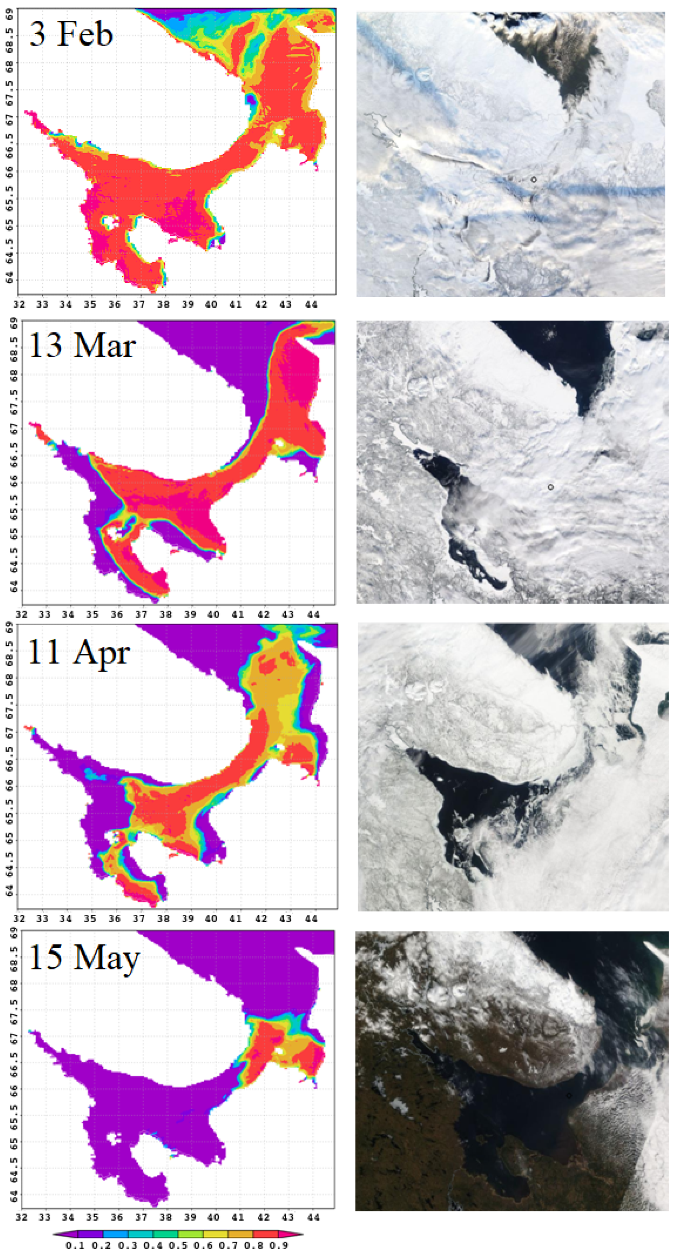
Figure 5 compares the results of sea–ice concentration modeling for 2011 (left column) with satellite images (https://multimaps.ru/, accessed on 2 June 2022) for the same day (right column). The model reproduces all stages of the sea ice life cycle, including duration of ice cover, formation of large areas of clear water in spring, order of ice melt from bays, and ice accumulation in some characteristic locations. Let us consider this in detail.
In January–February, almost the entire White Sea water area is covered with floating ice. Melting begins in March. Vast areas of open water are formed and ice is carried into the Barents Sea. The wind plays a key role in this process [41]. Polynyas form along the shores, and ice is pressed against the right-hand coasts of the bays.
In February, the sea is almost completely covered with ice; its destruction begins in March. It can be seen in the figure that in March in the northern part of the sea and along the western coast extensive polynyas are formed: this is reproduced by numerical simulation. The most complicated process of stage-by-stage sea clearance from ice in spring is also correct, as shown by the images for April and May: landfast ice stays in the bay tops and shallow bays; floating ice accumulates in straits during its motion in the north-eastern direction. Figure 5 demonstrates all these observed stages.
In the last decade of April, about of the area has been ice-free. The only remaining ice is in the northeastern part of the sea, also along the coast. By early summer, the White Sea is completely free of ice. However, although on average this pattern is typical, the life cycle of ice is characterized by considerable spatial and temporal variability.
According to [41], the fraction of ice that leaves the White Sea is significant: up to 50–80%. This fraction, as well as the amount of matter carried away by ice, is difficult to estimate accurately from observational data, and here numerical models can be particularly useful.
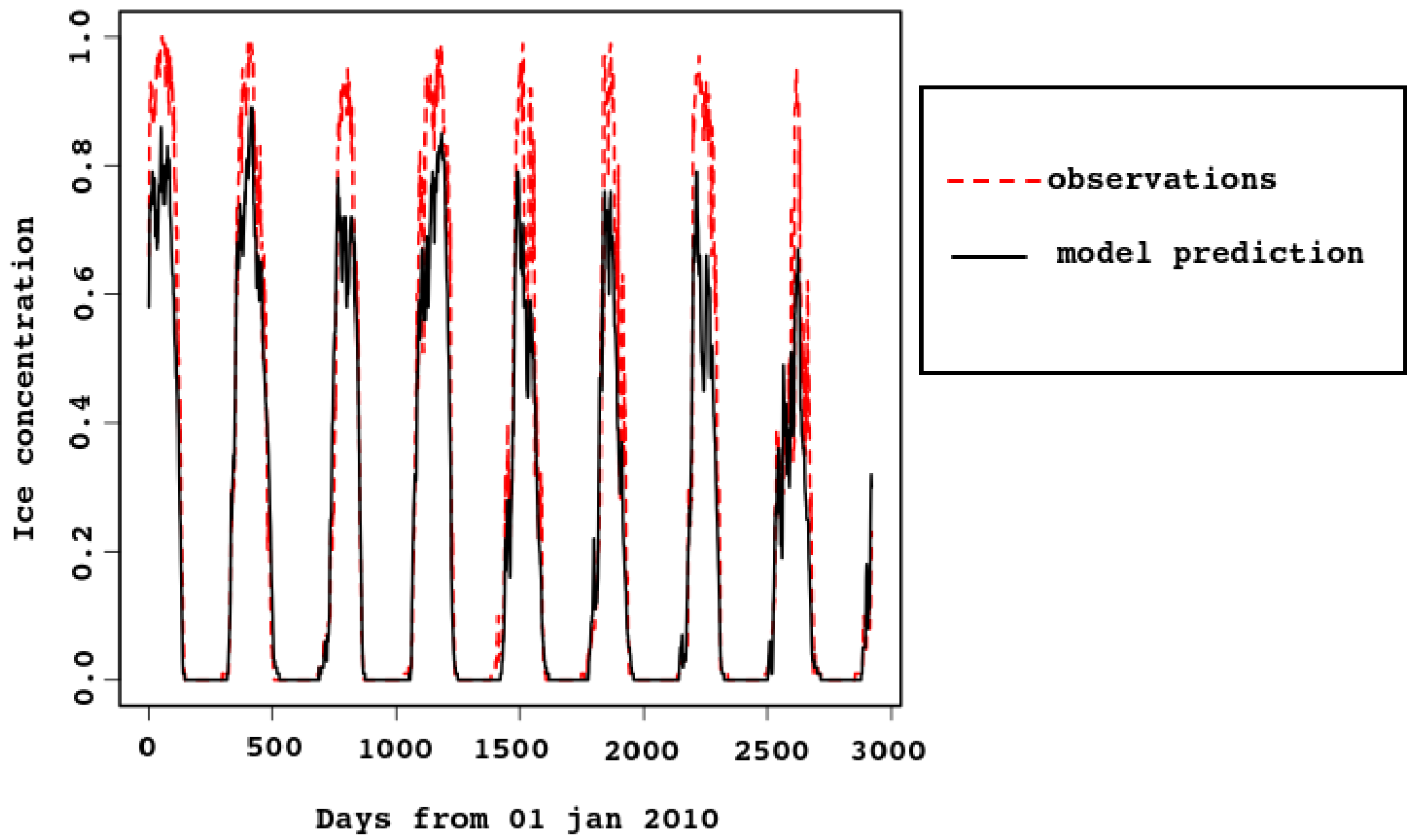
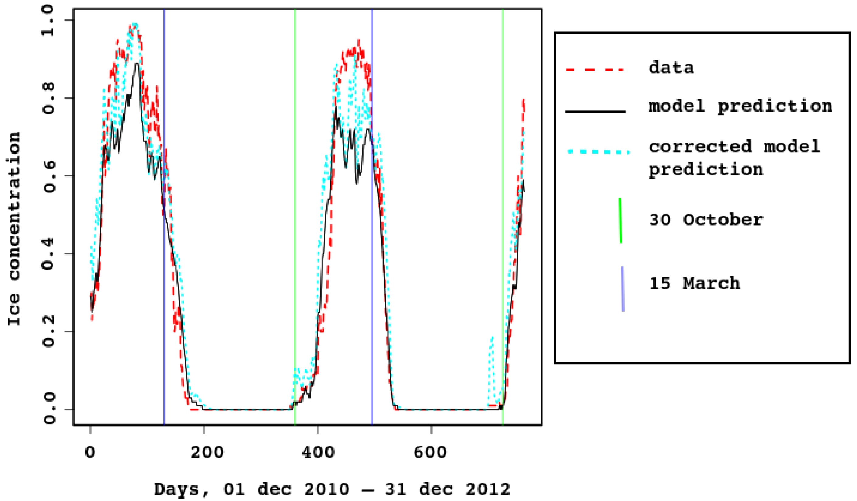
In Figure 3 and Figure 4, ice concentration for the entire sea is compared with the model result. The observed [6] values were obtained from satellite data. For spatial resolution km, a cell was considered to be filled with ice if there was ice in it. In the model, the grid cells have similar size (approximately km), each containing some ice concentration value from 0 to 1. This explains why the observed ice concentration is higher when the ice cover is maximal. For example, look at Figure 5, the first row (3 February). Most of the model map has sea–ice concentration between and , which means that the proportion of open water between ice flows is between 10 and 20%. The algorithm marks this area as 100% ice cover. In Figure 4, the cyan dotted line is added for the ice concentration computed in this way, with the 25% threshold: a grid cell with higher ice concentration is counted as ice-filled. Vertical lines mark 30th of October and 15th of March.
Note that timing of sea–ice freezing and melting is reproduced very well, although it is not built into the model. This proves that the heat balance in the model is described correctly.
As there are strong tidal currents, possibly enforced by wind, sea–ice concentration might reduce quickly for a short time due to ridging. This is clearly seen in Figure 4, both in model and satellite data. In the latter, the effect is smoothed by the algorithm (as already discussed), because ice-filled cells are considered full.
Figure 3.
Area-average sea–ice concentration, predicted by the model and estimated from the satellite data. Time span is 2010–2017.
Figure 3.
Area-average sea–ice concentration, predicted by the model and estimated from the satellite data. Time span is 2010–2017.

Figure 4.
Area-average sea–ice concentration, predicted by the model and estimated from the satellite data, 2011–2012.
Figure 4.
Area-average sea–ice concentration, predicted by the model and estimated from the satellite data, 2011–2012.

Multi-year simulations and satellite data were compared statistically. Linear regression of the observed time series N (average daily ice concentration) to the modeled M gives
with confidence below . The residuals are to with the median of and residual standard error of , . Thus, the Pearson correlation between the two time series is high (), but both time series are subject to seasonal fluctuations. To account for this, the series were filtered with a moving average over the year and repeated the same analysis for the filtered series.
Figure 5.
Sea–ice concentration, predicted by the model (left) and seen from a satellite (right), for the same dates of the year 2011.
Figure 5.
Sea–ice concentration, predicted by the model (left) and seen from a satellite (right), for the same dates of the year 2011.

The 95% confidence interval for the Pearson correlation is , the linear regression is
with confidence below . The residuals are to , with the median and residual standard error , .
Such qualitative predictability is due not only to the fact that the model describes ice dynamics well enough, but also to forcing, i.e., air temperature, insolation, etc. It is known that the White Sea reacts quickly to forcing [1].
As for sea ice thickness, there is no measurement data. The book [1] describes ice thickness by categories: gray (10–15 cm), gray-white (15–30 cm), and white (30–70 cm) ice. White and gray-white ice predominate throughout the sea in February, but ice ridges and hummocks are found everywhere in the sea. The model gives an average ice thickness of 70–80 cm, including thick ridged ice. In March, the winds usually blow eastward, forming open water areas along the west coast of the sea; this is well reproduced by the model.
The ecosystem model is difficult to tune because it requires a lot of computational power. Initial results seem reasonable. Let us compare a typical year with typical measurements at the Moscow State University biological station (shown in Figure 1).
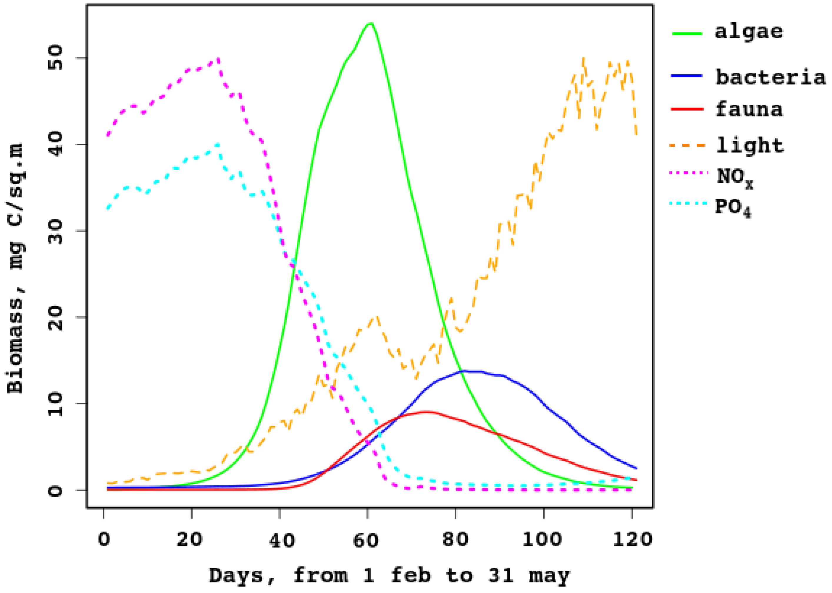
The model can simulate the production of sea–ice algae, bacteria, and fauna, and predicts growth (bloom) in March and decay in April–May. Samples collected at the end of March 2007–2008 [21] showed that ice algae and non-photosynthetic bacteria composed 90–96% and –10% of the total ice inhabitant biomass, respectively. In the model data these fractions change during the ice season from 10% to 90% and 5% to 70%; in March, the fraction of algae in the biomass changes from 82% to 94%, while that of bacteria is in the 4–13% range. Figure 6 compares daily biomass of algae, non-photosynthetic bacteria in sea ice, and sea–ice fauna for the range from February to May. Additionally shown is the illumination under the ice (it is normed, the maximum corresponds to W/m). Additionally, nutrient concentrations are shown (normed, maxima are mmole/m for nitrates, magenta line, and mmole/m for , cyan line). They prove that nutrients are limiting at the late stage of the ice period, while light is important at the early stage. This is not typical for polar ecosystems [25], but it is so in the Baltic [25] and the White seas.
The data show strong variability; for example, [21] reports the range 21–194 mg C/m for algae and –34 for bacteria, and average column values are 185 mg C/m and , respectively.
As shown in Figure 6, the model gives lower values; this is explained by the strong dependence of the bloom on the properties of the sea ice. In spring, when there is enough light, not only does the ice melt, but it is also carried away from the bay where the biostation is located (see Figure 1 and Figure 5). The model does not explicitly describe the landfast ice, while measurements are taken from it. In addition, ice thickness, ice transparency, and the presence of snow are extremely important and change rapidly during this short bloom period.
Figure 6 shows that the model reflects the trophic relations in the sea–ice brine-filled cavities: first the autotrophic algae start producing biomass; then heterotrophic organisms start grazing and eating organic remains, so the secondary production replaces the primary one. When the algal biomass reduces almost to zero, organic matter is utilized up to complete melt of the ice. The new ice contains some organic matter, captured from the water, but temperature and brine volume are too low, so activity of the heterotrophic fauna and bacteria is also low.
The authors of [42] studied the effects of river plumes on chlorophyll dynamics. We doubt that rivers are responsible for this underestimation of the model, since the only river with an estuary in the bay considered in the model is the Kovda; its flow is quite low compared to other rivers. Additionally, in winter, nutrients brought in by rivers accumulate in the water column and are available for pelagic blooms. Nutrients in sea ice are captured in the fall and therefore do not depend on instantaneous river runoff.
Figure 6.
Sea–ice model biomass of algae, bacteria, and fauna, for days from 31 Jan to 31 May.

It is interesting to compare the model with sea–ice ecology and the one with passive sea ice. In the latter, sea ice blocks light and influences the initial bloom significantly. In the former, additional effects are present: some matter is captured by forming ice and transported along the sea. Also, inorganic biogenic matter is transformed into organic and returned into water, and this is quickly done during several days in spring, when the light is already sufficient for photosynthesis and the ice is still present.
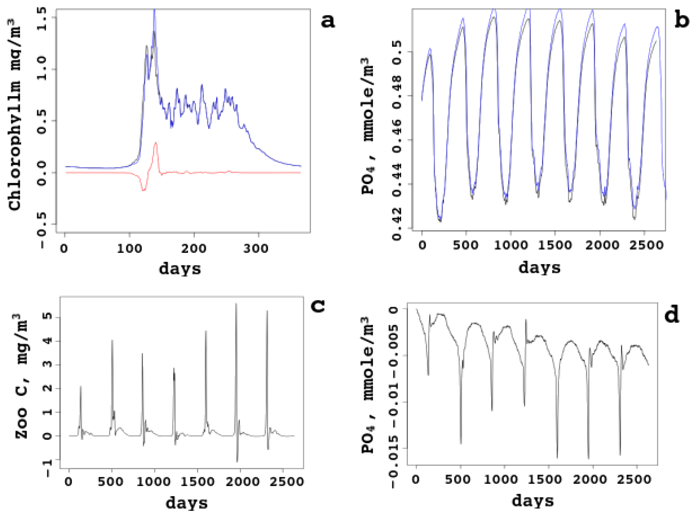
In Figure 7, daily surface biogeochemical concentrations for the whole sea are compared with sea–ice ecology taken into account and not taken. The bloom starts in April earlier, just one day, and the first peak is higher. However, the second peak is lower, because less nutrients are left and pressure from heterotrophic plankton is higher. Starting from June, the chlorophyll (subfigure a) dynamics becomes identical: sea–ice influence is “forgotten” by the chlorophyll (and the autotrophic biomass). On the other hand, nutrients (subfigures b and d compare the lines and give the difference, respectively) are always higher in the model with no sea–ice ecology, though the difference does not grow (no accumulation effect). The reason is clear: some inorganic matter is captured by the ice and taken away from the sea; some matter is converted into organic matter and returned to the pelagic cycle in this form. Zooplankton biomass (subfigure c) is also higher most of the time, because heterotrophic organisms have access to more organic matter released from the melting sea ice.
This shows that the ecology of the sea ice can be ignored in the model of the White Sea without a noticeable decrease of the model skill; however, some changes might be of importance, in particular, the earlier bloom and the influence on the second peak. Joined together with warming and random factors (like less clouds), sea–ice ecology can be among the explanations for observed time dependence of the biomass, chlorophyll, and other ecological quantities.
A peculiarity of the White Sea is the presence of ice of various origins in all parts of the sea throughout the winter: freshwater ice, saltwater ice, and frozen snow [41]. Almost everywhere there are ridges and hummocks. Ice grows not only downward due to water freezing, but also upward due to water-soaked snow. In the White Sea these processes are comparable; sometimes the ice grows upwards and stops growing downwards. The biologically active layer in this case may be more complex than in the model. Measurements showed the presence of biological activity in the upper, lower, and middle parts of the ice samples.
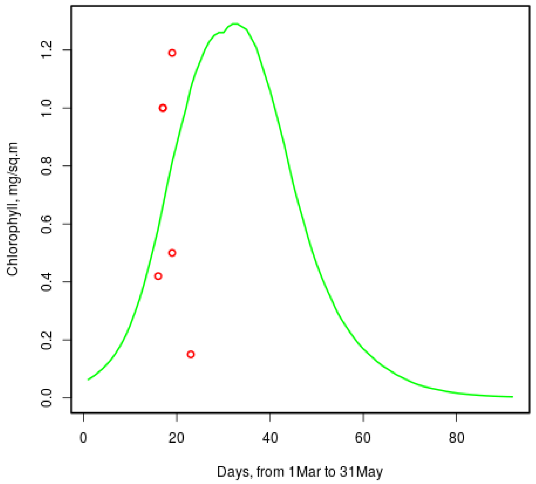
Chlorophyll-a concentrations reported in [9] range from to over 4 mg per m in late March; the model gives similar values to those shown in Figure 8. Red circles show measured [9] values for the same dates of 2013 and 2014. One more value () is not seen: it is for the 20th March.
Model chlorophyll dynamics is comparable to station data (in the Baltic Sea) in [25]. The chlorophyll concentration in Figure 8 resembles the line for “diatoms” (which is actually the total algal biomass) in Figure 9 in [25]. The decay there is faster, because the Baltic sea is ice-free by mid-April, while the White Sea usually contains some ice until the end of May. The White-sea ice seems to be more productive: the peak is mg per m,25] reports . Both values are supported by observations.
Changes in the ice ecosystem are very rapid: according to [21], primary productivity increased 40-fold in just two days in early April. Snow and ice melting and increased solar radiation create favorable, though short-lived, conditions for the primary production of sea ice.
Figure 8.
Model chlorophyll-a concentration in sea ice of a typical year and measured values [9] (red circles).
Figure 8.
Model chlorophyll-a concentration in sea ice of a typical year and measured values [9] (red circles).

4. Conclusions
The JASMINE numerical model was enriched by the sea–ice ecology submodel. The general sea circulation model and the Biogeochemical Flux Model were coupled online, i.e., with data exchange at each time step and advection and diffusion of biological tracers done by the same algorithms as for temperature, salinity, and sea–ice two-dimensional fields. Ice ridging parameter was tuned for better simulation of sea–ice dynamics. This the only comprehensive numerical model of the White Sea. Reproduction of sea–ice characteristics is discussed; all stages of the ice life cycle are shown to be reproduced correctly: ice formation in bays, increase of the ice-covered area, appearing of free-water regions, ice melting. It is important, that the timing is in good agreement with the results of satellite observations, which proves that the heat balance is correctly described in the model. As for the ecology of sea ice, numerical simulations agree with the scarce observation data on chlorophyll-a, biogenic elements, and biomass in the ice of this sea. Light is shown to be limiting at the beginning of the bloom; nutrient limitation is in the second half, up to the ice melt. This is not typical for the Arctic sea–ice ecology, but it is so in the Baltic, as well as in the White Sea. Numerical experiments showed that sea–ice ecology does not change the pelagic ecology description much; however, earlier bloom and different height of the algal biomass/chlorophyll peaks can be explained and taken into account.
Author Contributions
Conceptualization, I.C. and A.T.; methodology, N.I., I.C. and A.T.; software, N.I. and I.C.; validation, A.T.; investigation, I.C.; resources, A.T.; data assembling, A.T.; writing—original draft preparation, I.C.; writing—review and editing, I.C., A.T. and N.I.; visualization, I.C.; supervision, N.I. All authors have read and agreed to the published version of the manuscript.
Funding
The study was funded through Russian Science Foundation grant No 22-27-20014 implemented in collaboration with Republic of Karelia authorities with funding from the Republic of Karelia Venture Capital Fund; N.Iakovlev worked under state order to the INM (121121400411-2).
Data Availability Statement
Used satellite images are available at https://multimaps.ru/, accessed on 2 June 2022.
Acknowledgments
The authors are grateful to the colleagues Tatiana Belevich, Paolo Lazzari, Letizia Tedesco for valuable discussions.
Conflicts of Interest
The authors declare no conflict of interest.
Abbreviations
The following abbreviations are used in this manuscript:
| BAL | Biologically Active Layer; |
| BFM | Biogeochemical Flux Model; |
| BFMSI | BFM with Sea Ice; |
| CICE | The Los Alamos sea ice model (“Sea ICE”); |
| EVP | Elliptic Visco-Vlastic sea ice rheology; |
| FEMAO | Finite-Element Model of the Arctic Ocean; |
| FESIM | Finite-Element Sea Ice Model; |
| INM | G. Marchuk’s Institute of Numerical Mathematics of RAS; |
| NOAA | National Oceanic and Atmospheric Administration, USA; |
| MODIS | Moderate Resolution Imaging Spectroradiometer; |
| MSU | Moscow State University; |
| NESDIS | National Environmental Satellite, Data, and Information Service, USA; |
| NSIDC | National Snow and Ice Data Center, USA; |
| RAS | Russian Academy of Sciences; |
| SLAE | System of Linear Algebraic Equations; |
| ZIN | Zoological Institute of RAS. |
The following symbols are used in the paper:
| The e-folding scale used to compute ice ridging | |
| A parameter of the ice-ridging model | |
| Thickness of the ridging ice | |
| z | The vertical coordinate, zero at the surface, grows downwards |
| T | Water freezing temperature |
| S | Water salinity |
| Factor in the linear relation | |
| , | Sea–ice temperature and salinity |
| , | Average sea–ice temperature and salinity over the ice column |
| Salinity of the brine inside cavities in sea ice | |
| Sea–ice porosity | |
| Average sea–ice porosity over the ice column | |
| The critical ice temperature: if , porosity is too low to support life | |
| , | Temperatures of the upper ice edge and ice-contacting water |
| Gradient of the linear vertical temperature profile | |
| Relative thickness of the biologically active layer of the sea ice | |
| Ice thickness | |
| N, M | The observed and modeled time series |
| The coefficient of determination | |
| Chemical formula: phosphorus oxide |
References
- Zdorovennov, R.; Nazarova, L.; Tolstikov, A.; Bashmachnikov, I.; Bobvlev, L.; Brizgalo, V.; Chernook, V.; Denisov, V.; Donchenko, V.; Druzhinin, P.; et al. White Sea. Its Marine Environment and Ecosystem Dynamics Influenced by Global Change; Springer: London, UK, 2005. [Google Scholar]
- Gluhovskoy, B. (Ed.) The White Sea. Reference Book “Seas of the USSR”; Hydrometeorology and Hydrochemistry of Seas of the USSR; Volume II, N.1: Hydrometeorological Conditions; Hydrometeoizdat: Leningrad, Russia, 1991. (In Russian) [Google Scholar]
- Brown, L.; Duguay, C. The response and role of ice cover in lake-climate interactions. Prog. Phys. Geogr. Earth Environ. 2010, 34, 671–704. [Google Scholar] [CrossRef]
- Efremova, T.; Palshin, N.; Zdorovennov, R. Long-term characteristics of ice phenology in Karelian lakes. Est. J. Earth Sci. 2013, 62, 33–41. [Google Scholar] [CrossRef]
- Tilling, R.; Ridout, A.; Shepherd, A. Near-real-time Arctic sea ice thickness and volume from CryoSat-2. Cryosphere 2016, 10, 2003–2012. [Google Scholar] [CrossRef] [Green Version]
- Baklagin, V. Spatio-temporal regularities of the White Sea ice regime formation. Adv. Oceanogr. Limnol. 2022, 13. [Google Scholar] [CrossRef]
- Chernov, I.; Tolstikov, A. The White Sea: Available Data and Numerical Models. Geosciences 2020, 10, 463. [Google Scholar] [CrossRef]
- Lisitsyn, A. (Ed.) The White Sea System; Scientific World: Moscow, Russia, 2012; Volume 2. [Google Scholar]
- Belevich, T.; Ilyash, L.; Milyutina, I.; Logacheva, M.; Goryunov, D.; Troitsky, A. Photosynthetic Picoeukaryotes in the Land-Fast Ice of the White Sea, Russia. Microb. Ecol. 2018, 75, 582–597. [Google Scholar] [CrossRef]
- Melnikov, I.; Dikarev, S.; Egorov, V.; Kolosova, E.; Zhitina, L. Structure of the coastal ice ecosystem in the zone of sea-river interactions. Oceanology 2005, 45, 511–519. [Google Scholar]
- Ilyash, L.V.; Zhitina, L.S.; Kudryavtseva, V.A.; Melnikov, I.A. Seasonal dynamics of algae species composition and biomass in the coastal ice of Kandalaksha Bay, the White Sea. J. Gen. Biol. 2012, 73, 459–470. [Google Scholar]
- Sazhin, A.; Zhitina, L.; Sergeeva, V.; Ratkova, T.; Bakhmet, I. Algae in the ice and water of the White Sea in winter–spring transition period. Issues Mod. Algol. 2014, 2, 522. [Google Scholar]
- Kudryavtseva, V.; Belevich, T.; Zhitina, L. Diatoms in the ice of Velikaya Salma straight of the White Sea before the spring algal bloom. MSU Vestn. 2017, 72, 63–69. [Google Scholar]
- Semenov, E.; Bulatov, M. Analysis of the Operative Model of Hydrophysical Field Results in the White Sea from July to August 2008. Dokl. Earth Sci. 2010, 432, 710–714. [Google Scholar] [CrossRef]
- Benkort, D.; Daewel, U.; Heath, M.; Schrum, C. On the Role of Biogeochemical Coupling Between Sympagic and Pelagic Ecosystem Compartments for Primary and Secondary Production in the Barents Sea. Front. Environ. Sci. 2020, 8, 548013. [Google Scholar] [CrossRef]
- Campbell, K.; Matero, I.; Bellas, C.; Turpin-Jelfs, T.; Anhaus, P.; Graeve, M.; Fripiat, F.; Tranter, M.; Landy, J.C.; Sanchez-Baracaldo, P.; et al. Monitoring a changing Arctic: Recent advancements in the study of sea ice microbial communities. Ambio 2022, 51, 318–332. [Google Scholar] [CrossRef] [PubMed]
- Tedesco, L.; Vichi, M.; Scoccimarro, E. Sea-ice algal phenology in a warmer Arctic. Sci. Adv. 2019, 5, eaav4830. [Google Scholar] [CrossRef] [PubMed] [Green Version]
- Lannuzel, D.; Tedesco, L.; van Leeuwe, M. The future of Arctic sea-ice biogeochemistry and ice-associated ecosystems. Nat. Clim. Change 2020, 10, 983–992. [Google Scholar] [CrossRef]
- Gordeev, V. Fluvial sediment flux to the Arctic Ocean. Geomorphology 2006, 80, 94–104. [Google Scholar] [CrossRef]
- Shevchenko, V.; Filippov, A.; Novigatskiy, A. Dispersed sedimentary matter of freshwater and sea ice. In The White Sea System; Nauchnyi Mir: Moscow, Russia, 2012; Volume 2, pp. 169–200. (In Russian) [Google Scholar]
- Sazhin, A.; Sapozhnikov, F.; Rat’kova, T.; Romanova, N.; Shevchenko, V.; Filippov, A. Spring Ice, Under/Ice Water and Ground Inhabitants of the White Sea in the Estuarine Zone of the Northern Dvina. Oceanology 2011, 51, 307–318. [Google Scholar] [CrossRef]
- Chernov, I.; Lazzari, P.; Tolstikov, A.; Kravchishina, M.; Iakovlev, N. Hydrodynamical and biogeochemical spatiotemporal variability in the White Sea: A modeling study. J. Mar. Syst. 2018, 187, 23–35. [Google Scholar] [CrossRef]
- Iakovlev, N. On the simulation of temperature and salinity fields in the Arctic Ocean. Izv. Atmos. Ocean. Phys. 2012, 48, 86–101. [Google Scholar] [CrossRef]
- Vichi, M.; Lovato, T.; Butenschön, M.; Tedesco, L.; Lazzari, P.; Cossarini, G.; Masina, S.; Pinardi, N.; Solidoro, C.; Zavatarelli, M. The Biogeochemical Flux Model (BFM): Equation Description and User Manual; BFM Report Series 1.2; BFM Version 5.2; The BFM System Team: Bologna, Italy, 2020. [Google Scholar]
- Tedesco, L.; Vichi, M.; Haapala, J.; Stipa, T. A dynamic biologically-active layer for numerical studies of the sea ice ecosystem. Ocean Model. 2010, 35, 89–104. [Google Scholar] [CrossRef]
- Flather, R. A tidal model of the northwest European continental shelf. Mem. De La Societe R. Des Sci. De Liege 1976, 6, 141–164. [Google Scholar]
- Danilov, S.; Wang, Q.; Timmermann, R.; Iakovlev, N.; Sidorenko, D.; Kimmritz, M.; Jung, T.; Schröter, J. Finite-Element Sea Ice Model (FESIM), version 2. Geosci. Model Dev. 2015, 8, 1747–1761. [Google Scholar] [CrossRef] [Green Version]
- Lipscomb, W.; Hunke, E.; Maslowski, W.; Jakacki, J. Ridging, strength, and stability in high-resolution sea ice models. J. Geophys. Res. 2007, 112, C03S91. [Google Scholar] [CrossRef]
- Hunke, E.; Lipscomb, W. CICE: The Los Alamos Sea Ice Model, Documentation and Software; Technical Report 3.1 LA-CC-98-16; Los Alamos National Laboratory: Los Alamos, NM, USA, 2004. [Google Scholar]
- Melnikov, A.; Korneeva, G.; Zhitina, L.; Shanin, S. Dynamics of Ecological–Biochemical Characteristics of Sea Ice in Coastal Waters of the White Sea. Biol. Bull. 2003, 30, 164–170. [Google Scholar] [CrossRef]
- Parkinson, C.; Washington, W.M. A large-scale numerical model of sea ice. J. Geophys. Res. 1979, 84, 311–337. [Google Scholar] [CrossRef]
- Bitz, C.M.; Fyfe, J.C.; Flato, G. Sea Ice Response to Wind Forcing from AMIP Models. J. Clim. 2001, 15, 522–536. [Google Scholar] [CrossRef]
- Patara, L.; Vichi, M.; Masina, S. Impacts of natural and anthropogenic climate variations on north pacific plankton in an Earth system model. Environ. Model. 2012, 244, 132–147. [Google Scholar] [CrossRef]
- Tedesco, L.; Piroddi, C.; Kamari, M.; Lynam, C. Capabilities of Baltic sea models to assess environmental status for marine biodiversity. Mar. Policy 2016, 70, 1–12. [Google Scholar] [CrossRef]
- Piroddi, C.; Teixeira, H.; Lynam, C.; Smith, C.; Alvarez, M.; Mazik, K.; Andonegi, E.; Churilova, T.; Tedesco, L.; Chifflet, M.; et al. Using ecological models to assess ecosystem status in support of the european marine strategy framework directive. Ecol. Indic. 2015, 58, 175–191. [Google Scholar] [CrossRef]
- Tedesco, L.; Vichi, M.; Thomas, D. Process studies on the ecological coupling between sea ice algae and phytoplankton. Ecol. Model. 2012, 226, 120–138. [Google Scholar] [CrossRef]
- Cossarini, G.; Querin, S.; Solidoro, C.; Sannino, G.; Lazzari, P.; Di Biagio, V.; Bolzon, G. Development of BFMCOUPLER (v1.0), the coupling scheme that links the MITgcm and BFM models for ocean biogeochemistry simulations. Geosci. Model Dev. 2017, 10, 423–1445. [Google Scholar] [CrossRef] [Green Version]
- Mussapa, G.; Zavatarelli, M.; Pinardi, N.; Celio, M. Management oriented 1-d ecosystem model: Implementation in the Gulf of Trieste (Adriatic Sea). Reg. Stud. Mar. Sci. 2016, 6, 109–123. [Google Scholar] [CrossRef] [Green Version]
- Vichi, M.; Lovato, T.; Gutierrez Mlot, E.; McKiver, W. Coupling BFM with Ocean Models: The NEMO Model (Nucleus for the European Modelling of the Ocean); Technical Report; BFM Consortium: Bologna, Italy, 2015. [Google Scholar]
- Tedesco, L.; Miettunen, E.; An, B.; Happala, J.; Kaartokallio, H. Long-term mesoscale variability of modelled sea-ice primary production in the northern Baltic sea. Elem. Sci. Anthr. 2017, 5, 5–29. [Google Scholar] [CrossRef] [Green Version]
- Pantulin, A. Ice concentration and sea ice of the White Sea according to observations. In The White Sea System; Nauchnyi Mir: Moscow, Russian, 2012; Volume 2, pp. 120–132. (In Russian) [Google Scholar]
- Kubryakov, A.; Stanichny, S.; Zatsepin, A. River plume dynamics in the Kara Sea from altimetry-based lagrangian model, satellite salinity and chlorophyll data. Remote Sens. Environ. 2016, 176, 177–187. [Google Scholar] [CrossRef]
Figure 1.
The model domain with bathymetry marked by color and White Sea boundary shown as the red line. The red and black dots mark the positions of biological stations: the MSU Biological Station and the Biological Station of the ZIN RAS.
Figure 1.
The model domain with bathymetry marked by color and White Sea boundary shown as the red line. The red and black dots mark the positions of biological stations: the MSU Biological Station and the Biological Station of the ZIN RAS.

Figure 2.
Stamukha: an iceberg run aground, in the mouth of the Onega river, March 2003. Photo made by the authors. The height of this heap was about 7 m from the water level.
Figure 2.
Stamukha: an iceberg run aground, in the mouth of the Onega river, March 2003. Photo made by the authors. The height of this heap was about 7 m from the water level.

Figure 7.
Sea-average surface daily quantities with and without sea–ice ecology. (a) Chlorophyll-a concentration (one year) and the difference. (b,d) Nutrients (), compared and the difference. (c) Zooplankton biomass (the difference).
Figure 7.
Sea-average surface daily quantities with and without sea–ice ecology. (a) Chlorophyll-a concentration (one year) and the difference. (b,d) Nutrients (), compared and the difference. (c) Zooplankton biomass (the difference).

Publisher’s Note: MDPI stays neutral with regard to jurisdictional claims in published maps and institutional affiliations. |
© 2022 by the authors. Licensee MDPI, Basel, Switzerland. This article is an open access article distributed under the terms and conditions of the Creative Commons Attribution (CC BY) license (https://creativecommons.org/licenses/by/4.0/).
Share and Cite
MDPI and ACS Style
Chernov, I.; Tolstikov, A.; Iakovlev, N. Simulating Dynamics and Ecology of the Sea Ice of the White Sea by the Coupled Ice–Ocean Numerical Model. Water 2022, 14, 2308. https://doi.org/10.3390/w14152308
AMA Style
Chernov I, Tolstikov A, Iakovlev N. Simulating Dynamics and Ecology of the Sea Ice of the White Sea by the Coupled Ice–Ocean Numerical Model. Water. 2022; 14(15):2308. https://doi.org/10.3390/w14152308
Chicago/Turabian StyleChernov, Ilya, Alexey Tolstikov, and Nikolay Iakovlev. 2022. "Simulating Dynamics and Ecology of the Sea Ice of the White Sea by the Coupled Ice–Ocean Numerical Model" Water 14, no. 15: 2308. https://doi.org/10.3390/w14152308
Note that from the first issue of 2016, this journal uses article numbers instead of page numbers. See further details here.