
Reconstruction of Hydrometeorological Data Using Dendrochronology and Machine Learning Approaches to Bias-Correct Climate Models in Northern Tien Shan, Kyrgyzstan

 , ,
, , 
Abstract
:1. Introduction
2. Materials and Methods
2.1. Materials
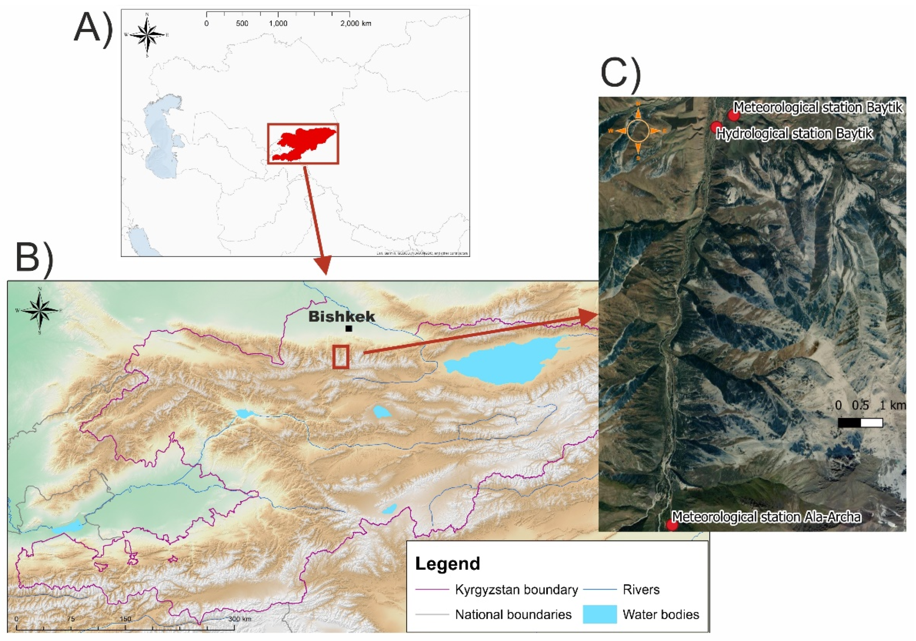
2.1.1. Study Site
2.1.2. Data
2.2. Methods
3. Results
3.1. Relationship between Discharge, Precipitation, Temperature, and Tree-Ring Width
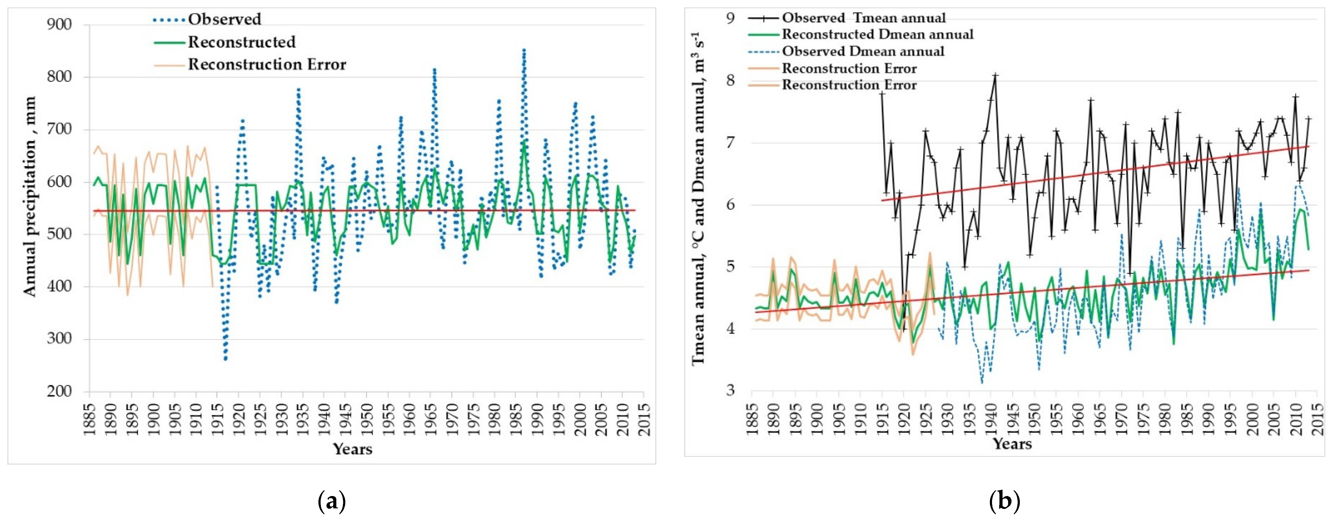
3.2. Hydrometeorological-Data Reconstruction and Validation
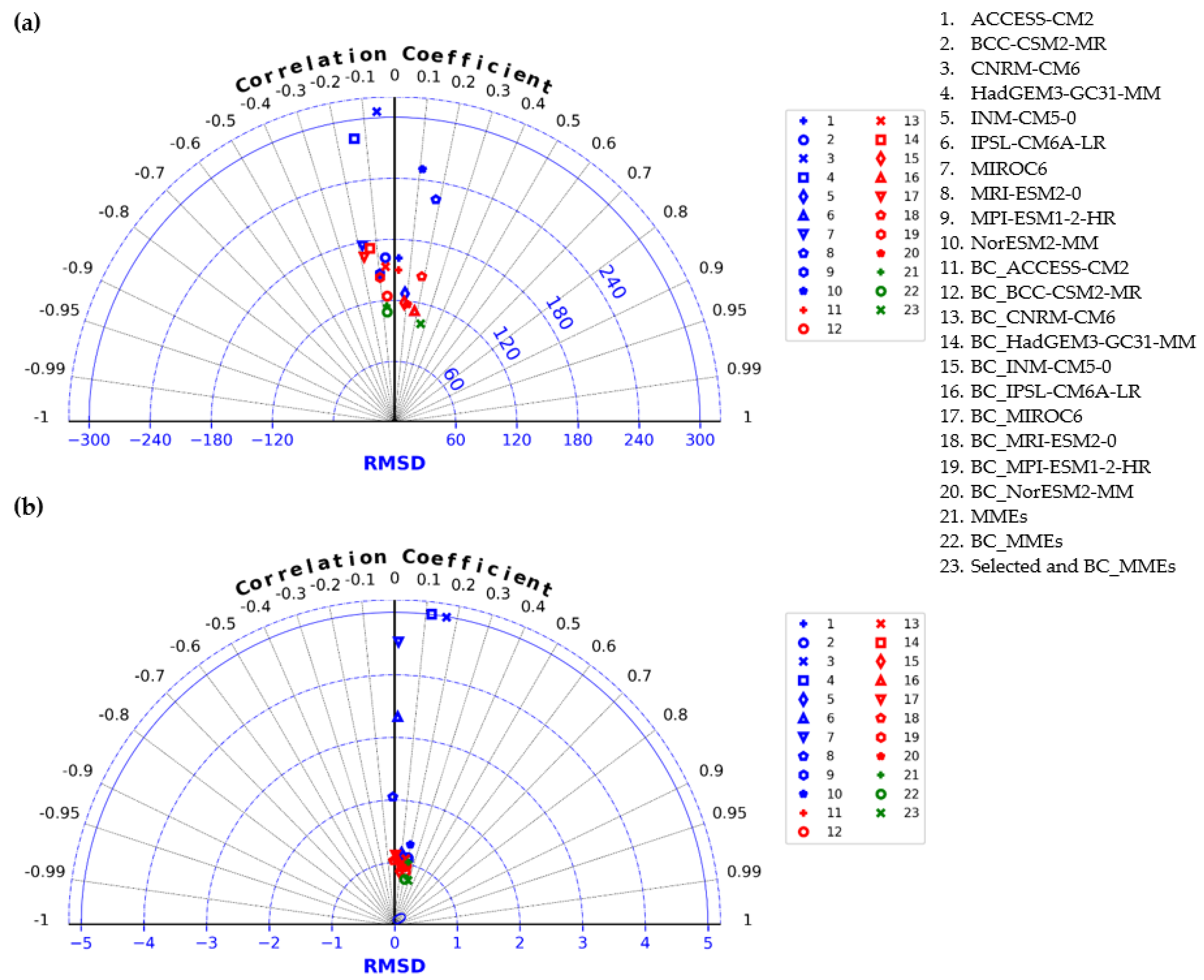
3.3. Performance Evaluation of CMIP5, CMIP6 GCMs, and CORDEX RCMs
3.4. Bias Corrections of GCMs
4. Discussion
5. Conclusions
- (1)
- Instrumental observations in Kyrgyzstan are insufficient for assessing long-term climate and hydrological changes. Due to their annual resolution and sensitivity to climate, tree rings provide reliable proxies that can be used to extend instrumental records, as shown in our findings between climate and discharge changes in drylands of Kyrgyzstan. We also provide qualitative information on long-term hydrologic variability in the region that can inform water managers, stakeholders, and decision-makers.
- (2)
- ML algorithms that combined RFR, KNN with HPT, and XgbR with HPT performed best, and these were used to reconstruct hydrometeorological data in Kyrgyzstan for the first time.
- (3)
- Increases in the average annual temperature and mean annual discharge of the Kashka-Suu River were associated with more rapid glacier melting; however, precipitation did not significantly change with time.
- (4)
- The CORDEX models best simulated precipitation and temperature over northern Tien Shan. These successfully replicated historical Tmeana (KGE = 0.24) and Pa (KGE = 0.24), due to their high spatial resolution (0.22°), indicating that spatial resolution plays a key role in complex mountain regions both for modeling atmospheric processes and model validation.
- (5)
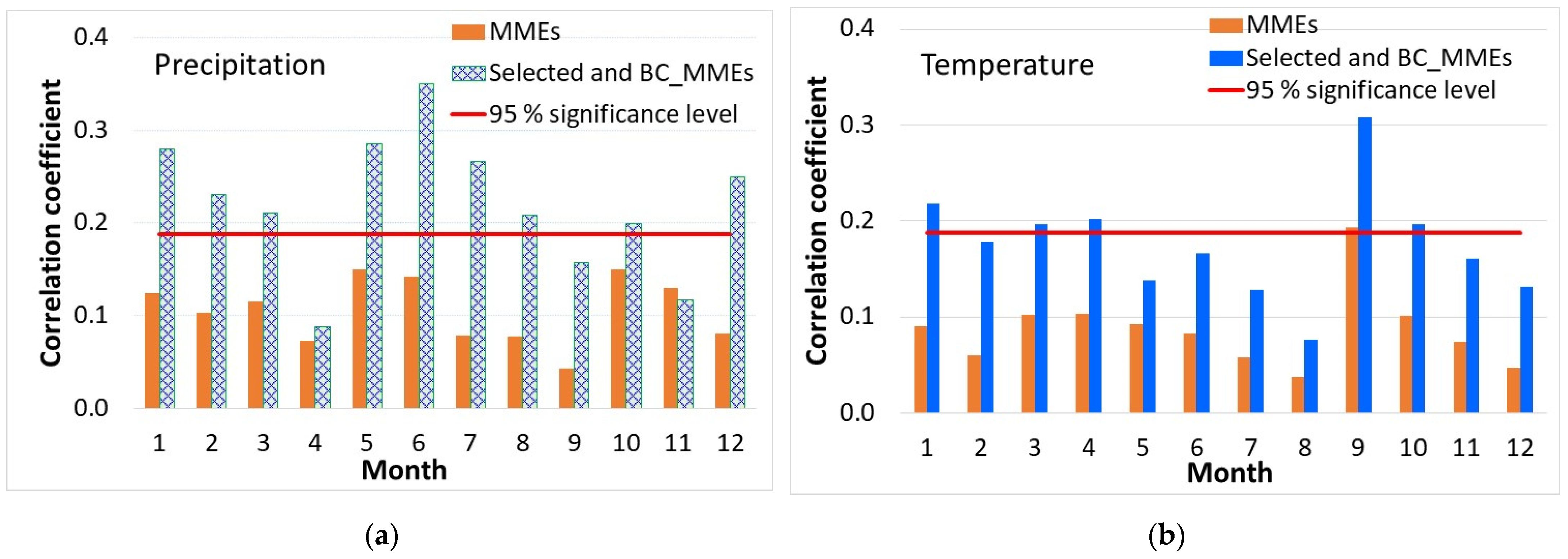
- Multi-model ensembles with selected GCMs and bias correction significantly increased performance of climate models.
Author Contributions
Funding
Institutional Review Board Statement
Informed Consent Statement
Data Availability Statement
Conflicts of Interest
References
- Immerzeel, W.W.; Van Beek, L.P.H.; Bierkens, M.F.P. Climate Change Will Affect the Asian Water Towers. Science 2010, 328, 1382–1385. [Google Scholar] [CrossRef] [PubMed]
- Ta, Z.; Yu, Y.; Sun, L.; Chen, X.; Mu, G.; Yu, R. Assessment of Precipitation Simulations in Central Asia by CMIP5 Climate Models. Water 2018, 10, 1516. [Google Scholar] [CrossRef] [Green Version]
- Alexander, L.V.; Zhang, X.; Peterson, T.C.; Caesar, J.; Gleason, B.; Klein Tank, A.M.G.; Haylock, M.; Collins, D.; Trewin, B.; Rahimzadeh, F.; et al. Global Observed Changes in Daily Climate Extremes of Temperature and Precipitation. J. Geophys. Res. Atmos. 2006, 111, 5109. [Google Scholar] [CrossRef] [Green Version]
- Sillmann, J.; Kharin, V.V.; Zwiers, F.W.; Zhang, X.; Bronaugh, D. Climate Extremes Indices in the CMIP5 Multimodel Ensemble: Part 2. Future Climate Projections. J. Geophys. Res. Atmos. 2013, 118, 2473–2493. [Google Scholar] [CrossRef]
- Pachauri, R.K.; Meyer, L.A. Climate Change 2014: Synthesis Report. In Contribution of Working Groups I, II, and III to the Fifth Assessment Report of the In-Tergovernmental Panel on Climate Change; IPCC: Geneva, Switzerland, 2014. [Google Scholar]
- Kastridis, A.; Stathis, D.; Sapountzis, M.; Theodosiou, G. Insect Outbreak and Long-Term Post-Fire Effects on Soil Erosion in Mediterranean Suburban Forest. Land 2022, 11, 911. [Google Scholar] [CrossRef]
- Wehner, M. Methods of Projecting Future Changes in Extremes. Water Sci. Technol. Libr. 2013, 65, 223–237. [Google Scholar]
- Climate Change Adaptation in Europe and Central Asia: AdApting to A ChAnging ClimAte for Resilient Development. Available online: www.adaptation-undp.org (accessed on 6 April 2022).
- Park, S.; Lim, C.H.; Kim, S.J.; Isaev, E.; Choi, S.E.; Lee, S.D.; Lee, W.K. Assessing Climate Change Impact on Cropland Suitability in Kyrgyzstan: Where Are Potential High-Quality Cropland and the Way to the Future. Agronomy 2021, 11, 1490. [Google Scholar] [CrossRef]
- Qiu, Y.; Feng, J.; Yan, Z.; Wang, J.; Li, Z. High-Resolution Dynamical Downscaling for Regional Climate Projection in Central Asia Based on Bias-Corrected Multiple GCMs. Clim. Dyn. 2022, 58, 777–791. [Google Scholar] [CrossRef]
- Huang, A.; Zhou, Y.; Zhang, Y.; Huang, D.; Zhao, Y.; Wu, H. Changes of the Annual Precipitation over Central Asia in the Twenty-First Century Projected by Multimodels of CMIP5. J. Clim. 2014, 27, 6627–6646. [Google Scholar] [CrossRef]
- Jiang, J.; Zhou, T.; Chen, X.; Zhang, L. Future Changes in Precipitation over Central Asia Based on CMIP6 Projections. Environ. Res. Lett. 2020, 15, 054009. [Google Scholar] [CrossRef]
- Bruyère, C.L.; Done, J.M.; Holland, G.J.; Fredrick, S. Bias Corrections of Global Models for Regional Climate Simulations of High-Impact Weather. Clim. Dyn. 2014, 43, 1847–1856. [Google Scholar] [CrossRef] [Green Version]
- Isaev, E.; Ajikeev, B.; Shamyrkanov, U.; Kalnur, K.; Maisalbek, K.; Sidle, R.C. Impact of Climate Change and Air Pollution Forecasting Using Machine Learning Techniques in Bishkek. Aerosol Air Qual. Res. 2022, 22, 210336. [Google Scholar] [CrossRef]
- Ahmed, K.; Sachindra, D.A.; Shahid, S.; Demirel, M.C.; Chung, E.S. Selection of Multi-Model Ensemble of General Circulation Models for the Simulation of Precipitation and Maximum and Minimum Temperature Based on Spatial Assessment Metrics. Hydrol. Earth Syst. Sci. 2019, 23, 4803–4824. [Google Scholar] [CrossRef] [Green Version]
- Wang, B.; Zheng, L.; Liu, D.L.; Ji, F.; Clark, A.; Yu, Q. Using Multi-Model Ensembles of CMIP5 Global Climate Models to Reproduce Observed Monthly Rainfall and Temperature with Machine Learning Methods in Australia. Int. J. Clim. 2018, 38, 4891–4902. [Google Scholar] [CrossRef]
- Srivastava, A.; Grotjahn, R.; Ullrich, P.A. Evaluation of Historical CMIP6 Model Simulations of Extreme Precipitation over Contiguous US Regions. Weather Clim. Extrem. 2020, 29, 100268. [Google Scholar] [CrossRef]
- Hassan, I.; Kalin, R.M.; White, C.J.; Aladejana, J.A. Selection of CMIP5 GCM Ensemble for the Projection of Spatio-Temporal Changes in Precipitation and Temperature over the Niger Delta, Nigeria. Water 2020, 12, 385. [Google Scholar] [CrossRef] [Green Version]
- Lin, C.Y.; Tung, C.P. Procedure for Selecting GCM Datasets for Climate Risk Assessment. Terr. Atmos. Ocean. Sci. 2017, 28, 43–55. [Google Scholar] [CrossRef] [Green Version]
- Nashwan, M.S.; Shahid, S. A Novel Framework for Selecting General Circulation Models Based on the Spatial Patterns of Climate. Int. J. Clim. 2020, 40, 4422–4443. [Google Scholar] [CrossRef]
- Smeraldo, S.; Bosso, L.; Salinas-Ramos, V.B.; Ancillotto, L.; Sánchez-Cordero, V.; Gazaryan, S.; Russo, D. Generalists yet Different: Distributional Responses to Climate Change May Vary in Opportunistic Bat Species Sharing Similar Ecological Traits. Mammal Rev. 2021, 51, 571–584. [Google Scholar] [CrossRef]
- Du, Z.; He, Y.; Wang, H.; Wang, C.; Duan, Y. Potential Geographical Distribution and Habitat Shift of the Genus Ammopiptanthus in China under Current and Future Climate Change Based on the MaxEnt Model. J. Arid Environ. 2021, 184, 104328. [Google Scholar] [CrossRef]
- Salehie, O.; Hamed, M.M.; Ismail, T.; Tam, T.H.; Shahid, S. Selection of CMIP6 GCM With Projection of Climate Over The Amu Darya River Basin. Res. Sq. 2021, 1–27. [Google Scholar] [CrossRef]
- Kastridis, A.; Kamperidou, V.; Stathis, D. Dendroclimatological Analysis of Fir (A. Borisii-Regis) in Greece in the Frame of Climate Change Investigation. Forests 2022, 13, 879. [Google Scholar] [CrossRef]
- Vitali, V.; Buntegen, U.; Bauhus, J. Seasonality Matters—The Effects of Past and Projected Seasonal Climate Change on the Growth of Native and Exotic Conifer Species in Central Europe. Dendrochronologia 2018, 48, 1–9. [Google Scholar] [CrossRef]
- Pederson, N.; Jacoby, G.C.; D’Arrigo, R.D.; Cook, E.R.; Buckley, B.M.; Dugarjav, C.; Mijiddorj, R. Hydrometeorological Reconstructions for Northeastern Mongolia Derived Form Tree Rings: 1651–1995. J. Clim. 2001, 14, 872–881. [Google Scholar] [CrossRef]
- Harley, G.L.; Maxwell, J.T.; Larson, E.; Grissino-Mayer, H.D.; Henderson, J.; Huffman, J. Suwannee River Flow Variability 1550–2005 CE Reconstructed from a Multispecies Tree-Ring Network. J. Hydrol. 2017, 544, 438–451. [Google Scholar] [CrossRef]
- Maxwell, R.S.; Harley, G.L.; Maxwell, J.T.; Rayback, S.A.; Pederson, N.; Cook, E.R.; Barclay, D.J.; Li, W.; Rayburn, J.A. An Interbasin Comparison of Tree-Ring Reconstructed Streamflow in the Eastern United States. Hydrol. Process. 2017, 31, 2381–2394. [Google Scholar] [CrossRef]
- Rao, M.P.; Cook, E.R.; Cook, B.I.; Palmer, J.G.; Uriarte, M.; Devineni, N.; Lall, U.; D’Arrigo, R.D.; Woodhouse, C.A.; Ahmed, M.; et al. Six Centuries of Upper Indus Basin Streamflow Variability and Its Climatic Drivers. Water Resour. Res. 2018, 54, 5687. [Google Scholar] [CrossRef]
- Strange, B.M.; Maxwell, J.T.; Robeson, S.M.; Harley, G.L.; Therrell, M.D.; Ficklin, D.L. Comparing Three Approaches to Reconstructing Streamflow Using Tree Rings in the Wabash River Basin in the Midwestern, US. J. Hydrol. 2019, 573, 829–840. [Google Scholar] [CrossRef]
- Woodhouse, C.A.; Lukas, J.J. Multi-Century Tree-Ring Reconstructions of Colorado Streamflow for Water Resource Planning. Clim. Change 2006, 78, 293–315. [Google Scholar] [CrossRef]
- Zhang, R.; Ermenbaev, B.; Zhang, H.; Shang, H.; Zhang, T.; Yu, S.; Chontoev, D.T.; Satylkanov, R.; Qin, L. Natural Discharge Changes of the Naryn River over the Past 265 Years and Their Climatic Drivers. Clim. Dyn. 2020 555 2020, 55, 1269–1281. [Google Scholar] [CrossRef]
- Chen, F.; Yuan, Y.; Wei, W.; Wang, L.; Yu, S.; Zhang, R.; Fan, Z.; Shang, H.; Zhang, T.; Li, Y. Tree Ring Density-Based Summer Temperature Reconstruction for Zajsan Lake Area, East Kazakhstan. Int. J. Climatol. 2012, 32, 1089–1097. [Google Scholar] [CrossRef]
- Zhang, R.; Qin, L.; Shang, H.; Yu, S.; Gou, X.; Mambetov, B.T.; Bolatov, K.; Zheng, W.; Ainur, U.; Bolatova, A. Climatic Change in Southern Kazakhstan since 1850 C.E. Inferred from Tree Rings. Int. J. Biometeorol. 2020, 64, 841–851. [Google Scholar] [CrossRef] [PubMed]
- Solomina, O.N.; Bradley, R.S.; Jomelli, V.; Geirsdottir, A.; Kaufman, D.S.; Koch, J.; McKay, N.P.; Masiokas, M.; Miller, G.; Nesje, A.; et al. Glacier Fluctuations during the Past 2000 Years. Quat. Sci. Rev. 2016, 149, 61–90. [Google Scholar] [CrossRef] [Green Version]
- Zhang, R.; Qin, L.; Yuan, Y.; Gou, X.; Zou, C.; Yang, Q.; Shang, H.; Fan, Z. Radial Growth Response of Populus Xjrtyschensis to Environmental Factors and a Century-Long Reconstruction of Summer Streamflow for the Tuoshigan River, Northwestern China. Ecol. Indic. 2016, 71, 191–197. [Google Scholar] [CrossRef]
- Zhang, R.; Wei, W.; Shang, H.; Yu, S.; Gou, X.; Qin, L.; Bolatov, K.; Mambetov, B.T.; Zhang, R.; Wei, W.; et al. A Tree Ring-Based Record of Annual Mass Balance Changes for the TS.Tuyuksuyskiy Glacier and Its Linkages to Climate Change in the Tianshan Mountains. QSRv 2019, 205, 10–21. [Google Scholar] [CrossRef]
- Yuan, Y.; Shao, X.; Wei, W.; Yu, S.; Gong, Y.; Trouet, V. The Potential to Reconstruct Manasi River Streamflow in the Northern Tien Shan Mountains (NW China). Tree-Ring Res. 2007, 63, 81–93. [Google Scholar] [CrossRef] [Green Version]
- Zhang, R.; Yuan, Y.; Gou, X.; Yang, Q.; Wei, W.; Yu, S.; Zhang, T.; Shang, H.; Chen, F.; Fan, Z.; et al. Streamflow Variability for the Aksu River on the Southern Slopes of the Tien Shan Inferred from Tree Ring Records. Quat. Res. 2016, 85, 371–379. [Google Scholar] [CrossRef]
- Panyushkina, I.P.; Meko, D.M.; Macklin, M.G.; Toonen, W.H.J.; Mukhamadiev, N.S.; Konovalov, V.G.; Ashikbaev, N.Z.; Sagitov, A.O. Runoff Variations in Lake Balkhash Basin, Central Asia, 1779–2015, Inferred from Tree Rings. Clim. Dyn. 2018, 51, 3161–3177. [Google Scholar] [CrossRef]
- Konovalov, V.G.; Maksimova, O.E. Reconstruction and prediction of water balance components from dendrochronological data for the naryn river basin (kyrgyzstan). Ice Snow 2015, 52, 87. [Google Scholar] [CrossRef]
- Zaginaev, V.; Ballesteros-Cánovas, J.A.; Erokhin, S.; Matov, E.; Petrakov, D.; Stoffel, M. Reconstruction of Glacial Lake Outburst Floods in Northern Tien Shan: Implications for Hazard Assessment. Geomorphology 2016, 269, 75–84. [Google Scholar] [CrossRef] [Green Version]
- Nabavi, S.O.; Haimberger, L.; Abbasi, E. Assessing PM 2.5 Concentrations in Tehran, Iran, from Space Using MAIAC, Deep Blue, and Dark Target AOD and Machine Learning Algorithms. Atmos. Pollut. Res. 2019, 10, 889–903. [Google Scholar] [CrossRef]
- Czernecki, B.; Marosz, M.; Jędruszkiewicz, J. Assessment of Machine Learning Algorithms in Short-Term Forecasting of PM 10 and PM 2.5 Concentrations in Selected Polish Agglomerations. Aerosol Air Qual. Res. 2021, 21, 200586. [Google Scholar] [CrossRef]
- Chang, Y.S.; Chiao, H.T.; Abimannan, S.; Huang, Y.P.; Tsai, Y.T.; Lin, K.M. An LSTM-Based Aggregated Model for Air Pollution Forecasting. Atmos. Pollut. Res. 2020, 11, 1451–1463. [Google Scholar] [CrossRef]
- Bolourani, S.; Brenner, M.; Wang, P.; McGinn, T.; Hirsch, J.S.; Barnaby, D.; Zanos, T.P.; Barish, M.; Cohen, S.L.; Coppa, K.; et al. A Machine Learning Prediction Model of Respiratory Failure within 48 Hours of Patient Admission for COVID-19: Model Development and Validation. J. Med. Internet Res. 2021, 23, e24246. [Google Scholar] [CrossRef] [PubMed]
- Hernández-Díaz, L.; Laprise, R.; Nikiéma, O.; Winger, K. 3-Step Dynamical Downscaling with Empirical Correction of Sea-Surface Conditions: Application to a CORDEX Africa Simulation. Clim. Dyn. 2017, 48, 2215–2233. [Google Scholar] [CrossRef] [Green Version]
- Done, J.M.; Holland, G.J.; Bruyère, C.L.; Leung, L.R.; Suzuki-Parker, A. Modeling High-Impact Weather and Climate: Lessons from a Tropical Cyclone Perspective. Clim. Change 2015, 129, 381–395. [Google Scholar] [CrossRef] [Green Version]
- Ehret, U.; Zehe, E.; Wulfmeyer, V.; Warrach-Sagi, K.; Liebert, J. HESS Opinions “Should We Apply Bias Correction to Global and Regional Climate Model Data”? Hydrol. Earth Syst. Sci. 2012, 16, 3391–3404. [Google Scholar] [CrossRef] [Green Version]
- Kretova, Z. Assessment of Climate Change in the Kyrgyz Republic under the IFAD Project “Livestock Development and Market-2”; IFAD: BIShkek, Kyrgyztsan, 2020. [Google Scholar]
- CORDEX-DKRZ Data Search|CORDEX-DKRZ|ESGF-CoG. Available online: https://esgf-data.dkrz.de/search/cordex-dkrz/ (accessed on 12 April 2022).
- Cmip6 Data Search|Cmip6|ESGF-CoG. Available online: https://esgf-node.llnl.gov/search/cmip6/ (accessed on 12 April 2022).
- CMIP5 Data Search|CMIP5|ESGF-CoG. Available online: https://esgf-node.llnl.gov/search/cmip5/ (accessed on 12 April 2022).
- Douglass, A.E. No Climatic Cycles and Tree Growth: A Study of the Annual Rings of Trees in Relation to Climate and Solar Activity; Carnegie Institute of Washington: Washington, DC, USA, 1919. [Google Scholar]
- Stoffel, M.; Corona, C. Dendroecological Dating of Geomorphic Disturbance in Trees. Tree-Ring Res. 2014, 70, 3–20. [Google Scholar] [CrossRef] [Green Version]
- RINNTECH—Technology for Tree and Wood Analysis-LINTAB™. Available online: http://www.rinntech.de/content/view/16/47/lang,english/index.html (accessed on 12 April 2022).
- Stoffel, M.; Bollschweiler, M. Tree-Ring Analysis in Natural Hazards Research—An Overview. Nat. Hazards Earth Syst. Sci. 2008, 8, 187–202. [Google Scholar] [CrossRef] [Green Version]
- Fritts, H.C. Tree Rings and Climate; Academic Press: Cambridge, MA, USA, 1976; ISBN 9780122684500. [Google Scholar]
- Mann, H.B. Nonparametric Tests Against Trend. Econometrica 1945, 13, 245. [Google Scholar] [CrossRef]
- Gupta, H.V.; Kling, H.; Yilmaz, K.K.; Martinez, G.F. Decomposition of the Mean Squared Error and NSE Performance Criteria: Implications for Improving Hydrological Modelling. J. Hydrol. 2009, 377, 80–91. [Google Scholar] [CrossRef] [Green Version]
- Taylor, K.E. Summarizing Multiple Aspects of Model Performance in a Single Diagram. J. Geophys. Res. Atmos. 2001, 106, 7183–7192. [Google Scholar] [CrossRef]
- Xiong, Y.; Ta, Z.; Gan, M.; Yang, M.; Chen, X.; Yu, R.; Disse, M.; Yu, Y. Evaluation of CMIP5 Climate Models Using Historical Surface Air Temperatures in Central Asia. Atmosphere 2021, 12, 308. [Google Scholar] [CrossRef]
- Isaev, E.K.; Mostamandi, S.; Ansikina, O. Evaluation of Parametrizations of Physical Processes in Hydrodynamic Model on the Quality of Atmospheric Processes Forecast in Areas with Complex Relief. Proc. Russ. State Hydrometeorol. Univ. 2015, 40, 30–41. [Google Scholar]
- Ozturk, T.; Turp, M.T.; Türkeş, M.; Kurnaz, M.L. Projected Changes in Temperature and Precipitation Climatology of Central Asia CORDEX Region 8 by Using RegCM4.3.5. Atmos. Res. 2017, 183, 296–307. [Google Scholar] [CrossRef]
- Harris, I.; Osborn, T.J.; Jones, P.; Lister, D. Version 4 of the CRU TS Monthly High-Resolution Gridded Multivariate Climate Dataset. Sci. Data 2020, 7, 109. [Google Scholar] [CrossRef] [Green Version]
- Singh, J.; Knapp, H.V.; Arnold, J.G.; Demissie, M. Hydrological modeling of the iroquois river watershed using HSPF and SWAT1. JAWRA J. Am. Water Resour. Assoc. 2005, 41, 343–360. [Google Scholar] [CrossRef]
- Moriasi, D.N.; Arnold, J.G.; van Liew, M.W.; Bingner, R.L.; Harmel, R.D.; Veith, T.L. Model evaluation guidelines for systematic quantification of accuracy in watershed simulations. Trans. ASABE 1983, 50, 885–900. [Google Scholar] [CrossRef]


| Institution, Country | Models-CMIP6 | Resolution | Models-CMIP5 | Resolution | CAS-CORDEX | Resolution |
|---|---|---|---|---|---|---|
| Australian Research Council Centre of Excellence for Climate System Science, Australia | ACCESS-CM2 | 1.87 × 1.25 | ACCESS13 | 1.90 × 1.20 | - | - |
| Beijing Climate Center, Beijing, China | BCC-CSM2-MR | 1.12 × 1.12 | BCC-CSM1.1-M | 2.80 × 2.80 | - | - |
| Institute for Numerical Mathematics, Russia | INM-CM5-0 | 2.00 × 1.50 | INMCM4.0 | 2.00 × 1.50 | - | - |
| Institute Pierre Simon Laplace(IPSL), France | IPSL-CM6A-lR | 2.50 × 1.27 | IPSL-CM5A-lr | 3.70 × 1.90 | - | - |
| Japan Agency for Marine-Earth Science and Technology (JAMSTEC), Japan | MIROC6 | 1.40 × 1.40 | MIROC5 | 1.40 × 1.40 | - | - |
| Max Planck Institute for Meteorology, Germany | MPI-ESM1-2-HR | 0.94 × 0.94 | MPI-ESM-MR | 1.90 × 1.90 | RegCM4-3.v5 | 0.44 × 0.44 |
| MPI-ESM1-2-LR | 1.87 × 1.86 | MPI-ESM-LR | 1.86 × 1.87 | REMO2015.v1 | 0.22 × 0.22 | |
| Meteorological Research Institute, Japan | MRI-ESM2-0 | 1.12 × 1.12 | MRI-ESM1 | 1.10 × 1.10 | - | - |
| Norwegian Climate Centre, Norway | NorESM2-MM | 1.00 × 1.00 | NorESM1-M | 1.89 × 2.50 | REMO2015.v1 | 0.22 × 0.22 |
| Met Office Hadley Centre, UK | HadGEM3-G | 1.00 × 1.00 | HadGEM2-ES | 1.25 × 1.87 | REMO2015.v1 | 0.22 × 0.22 |
| - | - | HadGEM2-ES | 1.25 × 1.87 | RegCM4-3.v5. | 0.44 × 0.44 | |
| National Centre for Meteorological Research, France | CNRM-CM6-1 | 1.00 × 1.00 | CNRM-CM5 | 1.40 × 1.40 | ALARO-0.v1 | 0.22 × 0.22 |
| Station Type Name | Meteorological, Baytik | Meteorological, Ala-Archa | Hydro-Logical Gauging, Baytik | - | |||||||
|---|---|---|---|---|---|---|---|---|---|---|---|
| Variable | Pa | Tmeana | Pa | Tmeana | Tmaxa | Tmina | Tmaxma | Tminma | Dmeana | Tree-Ring Width | |
| MeteorologicalBaytik | Pa | 1 | −0.07 | 0.83 | −0.21 | −0.36 | 0.44 | −0.2 | 0.22 | 0.04 | 0.47 |
| Tmeana | −0.07 | 1 | −0.05 | −0.05 | −0.01 | 0.19 | 0.57 | 0.48 | 0.36 | −0.26 | |
| MeteorologicalAla-Archa | Pa | 0.83 | −0.05 | 1 | −0.21 | −0.44 | 0.45 | −0.3 | 0.09 | −0.09 | 0.6 |
| Tmeana | −0.21 | −0.05 | −0.21 | 1 | 0.19 | −0.12 | 0.02 | −0.08 | 0.24 | −0.26 | |
| Tmaxa | −0.36 | −0.01 | −0.44 | 0.19 | 1 | −0.13 | 0.22 | −0.01 | 0.16 | −0.46 | |
| Tmina | 0.44 | 0.19 | 0.45 | −0.12 | −0.13 | 1 | −0.24 | 0.39 | −0.24 | 0.46 | |
| Tmaxma | −0.2 | 0.57 | −0.3 | 0.02 | 0.22 | −0.24 | 1 | 0.3 | 0.34 | −0.39 | |
| Tminma | 0.22 | 0.48 | 0.09 | −0.08 | −0.01 | 0.39 | 0.3 | 1 | 0.29 | −0.02 | |
| Hydrological Gauging Baytik | Dmeana | 0.04 | 0.36 | −0.09 | 0.24 | 0.16 | −0.24 | 0.34 | 0.29 | 1 | 0.14 |
| - | Tree-ring width | 0.47 | −0.26 | 0.60 | −0.26 | −0.46 | 0.46 | −0.39 | −0.02 | 0.14 | 1 |
| Station, Variable, Unit | Metrics | LR | XgbR with HPT | RFR with HPT | KNN with HPT | LaR | DTR with HPT | ANN |
|---|---|---|---|---|---|---|---|---|
| Meteorological, Baytik, Pa, mm | MAE | 70.8 | 60.9 | 69.4 | 59.7 | 70.6 | 77.8 | 70.6 |
| RMSE | 89.2 | 77.5 | 86.1 | 75.9 | 89.3 | 101.4 | 89.3 | |
| Meteorological, Ala-Archa, Pa, mm | MAE | 39.2 | 31.2 | 25.6 | 38.1 | 42.5 | 33.3 | 38.1 |
| RMSE | 49.7 | 41.3 | 33.1 | 50.4 | 53.8 | 44.7 | 50.4 | |
| Meteorological, Ala-Archa, Tmaxa, °C | MAE | 1.3 | 0.9 | 1.1 | 1.1 | 1.3 | 1.2 | 1.2 |
| RMSE | 1.6 | 1.2 | 1.4 | 1.3 | 1.7 | 1.4 | 1.4 | |
| Meteorological, Ala-Archa, Tmina, °C | MAE | 1.6 | 1.2 | 1.3 | 1.2 | 1.6 | 1.4 | 1.5 |
| RMSE | 2.0 | 1.5 | 1.7 | 1.6 | 2.0 | 1.8 | 1.9 | |
| Meteorological, Ala-Archa, Tmaxma, °C | MAE | 0.7 | 0.6 | 0.6 | 0.5 | 0.7 | 0.5 | 0.7 |
| RMSE | 0.8 | 0.7 | 0.7 | 0.6 | 0.8 | 0.7 | 0.8 | |
| Meteorological, Ala-Archa, Tminma, °C | MAE | 0.6 | 0.5 | 0.4 | 0.7 | 0.6 | 0.7 | 0.6 |
| RMSE | 0.8 | 0.6 | 0.5 | 0.8 | 0.8 | 0.8 | 0.8 | |
| Hydrological Gauging, Baytik, Dmeana, m3 s−1 | MAE | 0.5 | 0.2 | 0.4 | 0.5 | 0.5 | 0.5 | 0.5 |
| RMSE | 0.6 | 0.1 | 0.5 | 0.6 | 0.6 | 0.6 | 0.6 |
| Models | Meteorological Station Baytik | Meteorological Station Ala-Archa | |||||||
|---|---|---|---|---|---|---|---|---|---|
| Pa | Tmeana | Pa | Tmeana | ||||||
| KGE | RMSE, mm/year | KGE | RMSE, °C/year | KGE | RMSE, mm/year | KGE | RMSE, °C/year | ||
| CMIP5 | ACCESS1-3 | 0.15 | 113 | 0.12 | 1.7 | 0.03 | 113 | −0.12 | 2.3 |
| BCC-CSM1-1m | 0.00 | 160 | 0.19 | 1.4 | −0.05 | 149 | −0.98 | 5.2 | |
| CNRM-CM5 | −0.13 | 160 | −0.73 | 1.6 | −0.20 | 149 | −0.62 | 2.1 | |
| HadGEM2-ES | 0.08 | 116 | 0.08 | 0.6 | 0.07 | 105 | 0.02 | 1.0 | |
| INMCM4.0 | −0.12 | 197 | −0.05 | 4.2 | −0.05 | 182 | −0.26 | 1.0 | |
| IPSL-CM5A-LR | −0.19 | 158 | −0.25 | 5.5 | −0.12 | 143 | −0.37 | 1.6 | |
| MIROC5 | −0.01 | 136 | −0.01 | 2.5 | 0.07 | 117 | −1.41 | 6.3 | |
| MPI-ESM-MR | −0.05 | 143 | 0.10 | 3.0 | −0.02 | 127 | 0.11 | 1.4 | |
| MRI_ESM1 | −0.08 | 156 | 0.17 | 0.9 | 0.03 | 145 | −0.69 | 4.2 | |
| NorESM1-M | −0.11 | 184 | 0.17 | 1.0 | −0.01 | 168 | −0.82 | 4.1 | |
| CMIP6 | ACCESS-CM2 | 0.13 | 112 | 0.06 | 1.1 | 0.03 | 128 | −0.85 | 4.5 |
| BCC-CSM2-MR | −0.13 | 162 | 0.18 | 1.1 | −0.06 | 147 | −0.85 | 4.6 | |
| CNRM-CM6 | −0.16 | 306 | −0.15 | 5.0 | −0.17 | 302 | −0.04 | 1.2 | |
| HadGEM3-GC31-MM | −0.24 | 282 | −0.16 | 5.0 | −0.25 | 274 | 0.03 | 1.3 | |
| INM-CM5-0 | 0.02 | 127 | 0.05 | 1.1 | 0.05 | 113 | −0.76 | 4.5 | |
| IPSL-CM6A-LR | 0.11 | 112 | −0.10 | 3.3 | 0.04 | 103 | −0.20 | 1.3 | |
| MIROC6 | −0.19 | 177 | −0.21 | 4.5 | −0.22 | 165 | −1.85 | 8.1 | |
| MPI-ESM1-2-LR | −0.17 | 170 | 0.06 | 3.2 | −0.17 | 153 | 0.08 | 1.2 | |
| MRI-ESM2-0 | 0.10 | 223 | −0.05 | 2.1 | 0.05 | 222 | −1.13 | 5.7 | |
| MPI-ESM1-2-HR | −0.11 | 147 | 0.19 | 1.1 | −0.16 | 135 | −0.39 | 3.3 | |
| NorESM2-MM | −0.02 | 251 | 0.18 | 1.3 | −0.05 | 242 | −0.90 | 4.9 | |
| CORDEX | ALARO-0.v1_CNRM | −0.15 | 268 | −0.38 | 4.6 | −0.43 | 326 | −1.09 | 4.8 |
| RegCm4-3v5_HadCEM2-ES | −0.11 | 298 | −0.01 | 3.9 | −0.22 | 308 | 0.01 | 0.9 | |
| RegCm4-3v5_MPI-ESM-MR | −0.35 | 315 | 0.24 | 2.6 | −0.39 | 321 | −0.07 | 1.7 | |
| REMO2015_HadGEM2-ES | 0.06 | 131 | −0.07 | 4.2 | 0.07 | 128 | 0.11 | 0.8 | |
| REMO2015_MPI-M-ESM-LR | 0.17 | 137 | −0.33 | 3.9 | 0.24 | 131 | −0.37 | 0.8 | |
| REMO2015_NCC-NorESM1-M | −0.08 | 164 | −0.03 | 3.6 | −0.11 | 160 | 0.02 | 1.0 | |
| Models | Baytik Meteorological Station | ||||||||
|---|---|---|---|---|---|---|---|---|---|
| Pa | Bias Corrected Pa | Tmeana | Bias Corrected Tmeana | ||||||
| KGE | RMSE, mm/year | KGE | RMSE, mm/year | KGE | RMSE, °C/year | KGE | RMSE, °C/year | ||
| CMIP6 | ACCESS-CM2 | 0.13 | 112 | 0.19 | 112 | 0.06 | 1.1 | 0.06 | 1.0 |
| BCC-CSM2-MR | −0.13 | 162 | −0.10 | 125 | 0.18 | 1.1 | 0.19 | 1.0 | |
| CNRM-CM6 | −0.16 | 306 | −0.06 | 153 | −0.15 | 5.0 | 0.13 | 1.1 | |
| HadGEM3-GC31-MM | −0.24 | 282 | −0.16 | 173 | −0.16 | 5.0 | 0.12 | 0.9 | |
| INM-CM5-0 | 0.02 | 127 | 0.04 | 118 | 0.05 | 1.1 | 0.06 | 0.9 | |
| IPSL-CM6A-LR | 0.11 | 112 | 0.11 | 110 | −0.10 | 3.3 | 0.01 | 1.1 | |
| MIROC6 | −0.19 | 177 | −0.10 | 165 | −0.21 | 4.5 | 0.00 | 1.1 | |
| MPI-ESM1-2-LR | −0.17 | 170 | −0.10 | 168 | 0.06 | 3.2 | 0.19 | 0.9 | |
| MRI-ESM2-0 | 0.10 | 223 | 0.15 | 146 | −0.05 | 2.1 | −0.01 | 1.0 | |
| MPI-ESM1-2-HR | −0.11 | 147 | −0.05 | 143 | 0.19 | 1.1 | 0.20 | 0.9 | |
| NorESM2-MM | −0.02 | 251 | 0.06 | 117 | 0.18 | 1.3 | 0.19 | 1.0 | |
| Mean | MMEs | −0.06 | 188 | 0.01 | 139 | 0.01 | 2.6 | 0.10 | 1.0 |
Publisher’s Note: MDPI stays neutral with regard to jurisdictional claims in published maps and institutional affiliations. |
© 2022 by the authors. Licensee MDPI, Basel, Switzerland. This article is an open access article distributed under the terms and conditions of the Creative Commons Attribution (CC BY) license (https://creativecommons.org/licenses/by/4.0/).
Share and Cite
Isaev, E.; Ermanova, M.; Sidle, R.C.; Zaginaev, V.; Kulikov, M.; Chontoev, D. Reconstruction of Hydrometeorological Data Using Dendrochronology and Machine Learning Approaches to Bias-Correct Climate Models in Northern Tien Shan, Kyrgyzstan. Water 2022, 14, 2297. https://doi.org/10.3390/w14152297
Isaev E, Ermanova M, Sidle RC, Zaginaev V, Kulikov M, Chontoev D. Reconstruction of Hydrometeorological Data Using Dendrochronology and Machine Learning Approaches to Bias-Correct Climate Models in Northern Tien Shan, Kyrgyzstan. Water. 2022; 14(15):2297. https://doi.org/10.3390/w14152297
Chicago/Turabian StyleIsaev, Erkin, Mariiash Ermanova, Roy C. Sidle, Vitalii Zaginaev, Maksim Kulikov, and Dogdurbek Chontoev. 2022. "Reconstruction of Hydrometeorological Data Using Dendrochronology and Machine Learning Approaches to Bias-Correct Climate Models in Northern Tien Shan, Kyrgyzstan" Water 14, no. 15: 2297. https://doi.org/10.3390/w14152297