Monitoring Changes in Land Use Land Cover and Ecosystem Service Values of Dynamic Saltwater and Freshwater Systems in Coastal Bangladesh by Geospatial Techniques

Abstract

Assessing and modeling the changes in land use and land cover (LULC) patterns and associated ecosystem service values (ESV) has become an important global agenda for formulating sustainable land management policies. Taking the coastal region of Bangladesh (CRB) as a case study, we utilized remote sensing and GIS techniques to analyze Landsat data of 1999 and 2019 to estimate the effect of LULC changes on the ESVs. The LULC classification, ESV quantification, and spatial variations were performed by semi-automated classification, per-unit value transfer, and spatial autocorrelation techniques, respectively. First, between 1999 and 2019, LULC altered dramatically (agricultural land and coastal wetlands decreased, while all other LULC types increased). Second, the total ESV decreased by 1.87%, which was mostly attributed to a 70% growth in both rural settlement and aquaculture/saltpan, and a 30% decline in both agricultural land and wetlands. Third, significant spatial correlation and moderately high spatial clustering were observed, which consisted mostly of mangrove forests, waterbodies, and wetland zones. Both high-high and low-low values increased, but spatial outliers remained unchanged. Conserving agricultural land should be prioritized in future land use plans of CRB to meet the ever-increasing food demands, control natural land conversion, and make land use sustainable.

1. Introduction

Ecosystem services (ES) are the state and mechanisms by which natural ecosystems and the species that make up those ecosystems support and satisfy human well-being [1,2,3]. ES may be defined as products and services that directly or indirectly enhance human survival. Provisioning, supporting, regulating, and cultural services are all examples of ES [4,5]. These ES take into account multifarious societal advantages. The changes in land use land cover (LULC) have been significant globally due to rising population, economic growth, and urban expansion over the past decades [6,7]. While humanity has changed the structure and pattern of LULC to acquire foods, fibers, fuel, and other supplies for thousands of years, the degree and speed of change have accelerated dramatically these days [8]. On earth, there is barely anything that remains unchanged [9]. Globally, forests are more generally converted into cropland, pastures, and growing areas. Annually, an estimated 13 million hectares of agricultural land expansion into forest lands is evidenced. Despite the significant increase in supply of food, fiber, wood, housing, and other critical requirements, the changing dynamics of LULC are associated with a decreased supply of many ES and an estimated 60% of the ES have been ruined during the last five decades [10].

The study of land cover is a potential utilization of remote sensing since sensors can detect the radiation that is reflected from the surface. This enables the quality of the land cover to be evaluated [11]. There is a connection between the study of ecosystem services and remote sensing because of the characterization of soil type, biomass, tree canopy, leaf area index (LAI), space-time monitoring of vegetation, and other factors [12,13,14,15,16]. These factors, along with others, enable us to identify and map the contribution and loss of ecosystem services from natural elements on the surface of the earth through the use of models, spectral indices, merging different sources, and other processes. In other words, remote sensing helps us to study ecosystem services [17]. The enhancement of remote sensing in terms of geographical, spectral, radiometric, and temporal resolution has increased its use by enabling the evaluation of ecosystem services [18,19]. This is one of the many benefits of these advancements. In the process of evaluating ecosystem services and determining how those services relate to decisions about land use, a broad range of methodologies and techniques have been uncovered [20].

Ecological economists who have been analyzing environmental resources using the profit-loss method are increasingly emphasizing ES evaluation. However, many ecosystem services are public goods, and their economic benefit is hard to measure as a marketable commodity, which is a major challenge for the assessment process of ecosystem services. Nevertheless, the monetary assessment of ES is an integrated and universal tool for determining and informing LULC change effects, and for campaigning, giving priority and concentrating on investment interest in conservation and management practices [6]. In addition, it may be necessary to measure ES and examine changes in its values that help the sustainable land use process, as they provide a valuable approach to determining trade-offs between alternative land use choices.

Several studies have been conducted in Bangladesh and across the world to track the influence of LULC alterations on the structure and functioning of ESV. Most of these studies indicated a moderate to large drop in ESV as a result of LULC alterations and urbanization, whereas others found absolutely no changes. ESV has also been found to be increasing in some investigations. The causes of such variances in ESV are both anthropogenic and natural factors. To begin with, in terms of rapid urbanization and industrialization, numerous changes in LULC occur at the same time, due to a variety of competing demands that are not restricted to urban sprawl. Reforestation and protection, natural protection, infrastructural development, comfort, and tourism and recreation are only a few of them [21,22]. Second, there is a strong link between ESV types and LULC usage [23,24]. The capacity to synthesize and apply the outcomes of these case studies to other places is limited due to their significant implications and distinct nature and characteristics. Among the natural processes, sea-level rise, salinity intrusion, and erosion are reported in Bangladesh [25,26]. As a result, it is critical to investigate the influence of LULC changes on ESV in order to inform policy- and decision-makers for sustainable planning and management as well as a safe ecological system.

There are several ways of quantifying the value of different ecosystem services, but the “benefit transfer” devised by Costanza et al. [2] is the most widely utilized. As far as service functions go, they divided the world’s ecosystems into 16 categories and 17 subtypes. When applied to Bangladesh, however, their findings have been widely planned. Bias exists in some circumstances, such as when agricultural ESV is understated and wetland ESV is overstated. Instead of developing countries such as Bangladesh, their ESV resembled the economic level of industrialized countries (e.g., the United States and European countries). Huq et al. [27] developed the equivalent per unit area for Bangladesh’s freshwater ecosystem services using the same methods proposed by Costanza et al. [2]. A poll of 200 ecologists was used to determine the equivalent weight factor. In some parts of coastal Bangladesh, equivalent per-unit-area values were combined with land use data to calculate ESV [27]. By coordinating the land cover types proportional to the biomes, LULC can operate as a proxy using this strategy. The latter then assigns economic values centered on a standard, which are subsequently adjusted locally and the coefficient values are determined. This method is a form of multi-criteria technique that allows the integration of multiple different metrics into a single monetary unit. This method also yields reliable and comparable findings, as well as an evaluation of change over time and across a varied urbanization standpoint. As a result, it provides a continuous mechanism for increasing knowledge over time from various study findings.

The current study focuses on the coastal region of Bangladesh (CRB). The CRB is a dynamic mix of saltwater and freshwater systems that provide economically valuable ecosystem services (ESs) to local communities but are under tremendous strain from both climate change and human activity [28]. Since 2009, Bangladesh’s economic development has accelerated to the point where it now embraces the vision for 2021 and 2041, making it one of the world’s fastest-developing areas [29]. As a result, the coastal regions have been subjected to harsh natural conditions, overconsumption, and loss of natural provisioning services, putting ecosystems and human well-being at risk. The Bangladesh government has taken a number of steps to ameliorate the country’s deteriorating environmental situation, including increasing forest cover and protecting high-yield agriculture. The key limiting element in the CRB’s social and economic sustainable growth is the provision of ES in an imbalanced manner. However, no studies in CRB have been done that give a full knowledge and estimation of the influence of such changes in land cover and policy on the ESs. As a result, the goals of this research were to (i) monitor and quantify the changes in LULC and ESVs of the CRB between 1999 and 2019; and (ii) analyze the spatial distribution and variations of ESVs across the CRB. To do so, Landsat images were processed and analyzed through the Semi-Automated Classification Plugin in QGIS 2.18.14. ESV was estimated following the unit value transfer method. Besides, spatial distribution patterns and changes were assessed through district-level mapping and categorization of the values of different ecosystem functions, and spatial autocorrelation. After that, the sensitivity coefficient was calculated to determine the value coefficient’s uncertainty. This study seeks to generate helpful information for rural-urban planners and decision-makers for regional coordination and sustainable development based on the findings.

The present article proceeds with a brief description of the study area and an explanation of the data and methods. This segment comprises the valuation and calculation of the ESV of the CRB. Finally, we folded up the presentation of the core findings of the study with their discussions and their possible implications.

2. Materials and Methods

2.1. Study Location

The Ganges–Brahmaputra–Meghna (GBM) river system and the Bay of Bengal dominate the geomorphology and hydrology of Bangladesh’s coastal zone. Bangladesh’s coastline zone (Figure 1) comprises 47,201 km², accounting for 32 percent of the country’s landmass and 19 districts (Jessore, Narail, Gopalganj, Shariatpur, Chandpur, Satkhira, Khulna, Bagerhat, Pirozpur, Jhalakati, Barguna, Barisal, Patuakhali, Bhola, Lakshmipur, Noakhali, Feni, Chittagong, and Cox’s Bazar). The coastal zone is home to around 35 million people, or 29 percent of the population [30]. Bangladesh’s coastal zone is divided into three sections based on geographic features: (a) the eastern zone; (b) the central zone; and (c) the western zone [31]. The semi-active delta is crisscrossed by many channels and streams in the western area, known as the Ganges tidal plain. The most vigorous and continuous accretion as well as erosion processes are seen in the central area. This zone includes the Meghna River Estuary. The eastern section is dominated by more stable steep terrain. The 710 km long coastline is made up of the intersection of different biological and economic systems, including mangroves (the world’s biggest mangrove forest encompasses 6017 square kilometers) and tidal flats. Estuaries, sea grass, around 70 islands, accreted land, beaches, a peninsula, agricultural communities, urban and industrial regions, and ports make up the island chain. Many of the people who live along the shore are impoverished, and they are vulnerable to both natural and manmade calamities. The primary natural catastrophes include sea-level rise, cyclones, storm surges, coastal flooding, salt intrusion, and land erosion, all of which are caused by climate change [32,33].

2.2. LULC Change Analysis

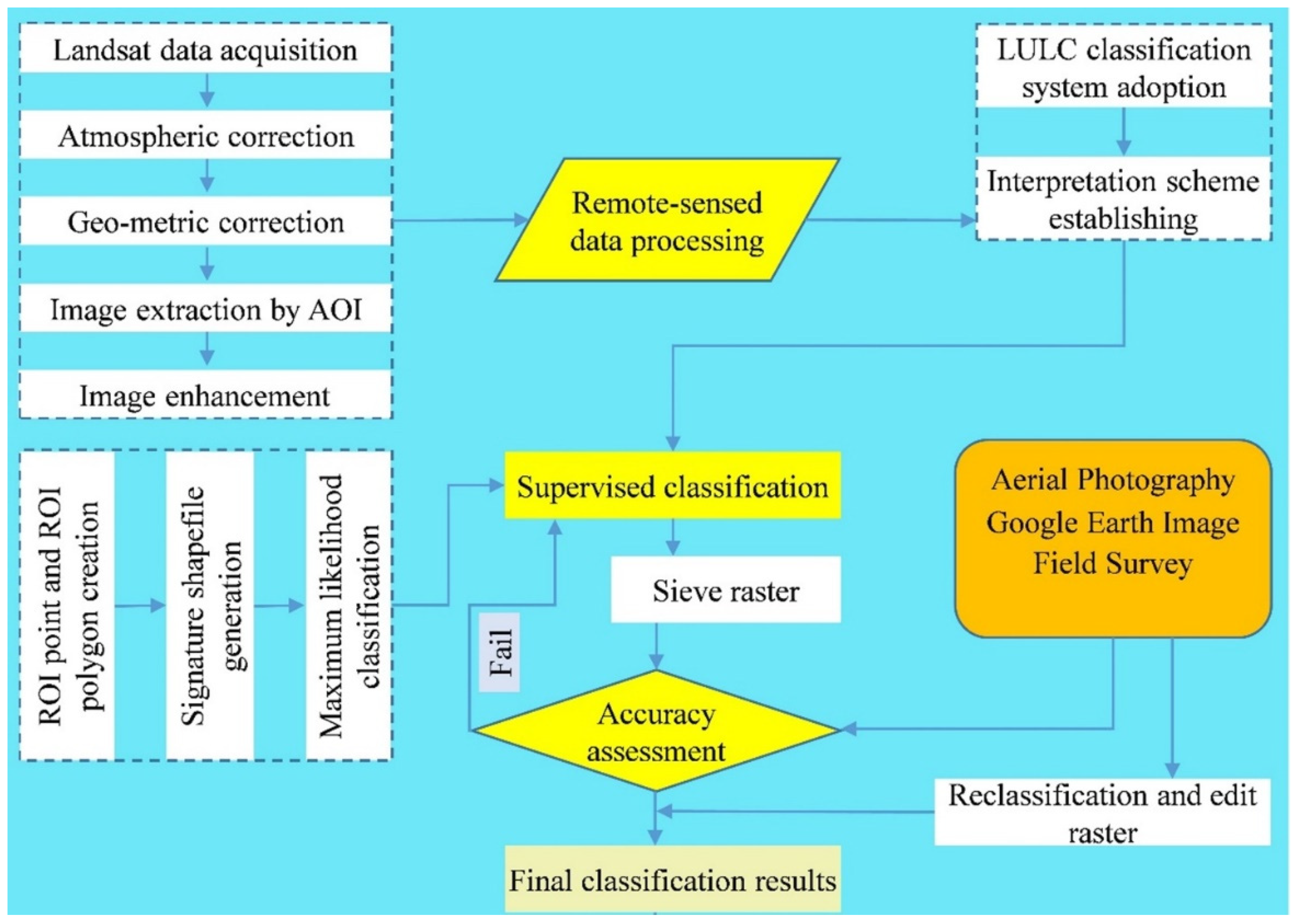
2.2.1. Satellite Data Acquisition and Classification

LSDS Science Research and Development database of the United States (https://espa.cr.usgs.gov/, accessed on 5 May 2021) was used to gather a total of eight LandsatTM and OLI-TIRS scenes (paths/row: 135/45, 135/46, 133/44, 133/45, 137/44, 137/45, 138/44, and 138/45) with a spatial resolution of 30 m × 30 m. For the years 1999 and 2019, a total of 16 scenes were utilized to analyze the LULC patterns. We only evaluated images captured during the dry season with a cloud cover of 0 percent in order to reduce data set disturbance. Furthermore, we developed a systematic procedure for processing Landsat images, which includes steps such as clipping images by study area shapefiles, stacking different bands, creating a mosaic of the multiband image, creating ROI and signature shapefiles, performing supervised maximum likelihood classification, and post-processing to improve the quality of misclassified data (Figure 2, Figures S1 and S2).

We considered 7 broad LULC forms (

Table 1. Land use and land cover classification scheme for CRB.

Type	Description
Agricultural land (AL)	Cultivated and uncultivated farmlands
Rural settlement and mixed vegetations (RSMV)	Land covered with woodland, trees in the soil forests, around homesteads and rural institutions, and mixed plantation forest vegetation along the roadside
Mangrove forest (MF)	Natural and plantation mangrove forest vegetation in the wetland and offshore areas
Coastal wetland (CW)	Mudflat, coastal flat, exposed soils in the riverine area, wetland, coastal marsh, and newly accreted land
Built-up (BU)	Residential, commercial, industrial, transportation, roads, mixed urban, and other forms of development land areas
Waterbody (WB)	River networks, canals, and active hydrological features
Aquaculture/ Salt pan (AS)	Flowing open waterbodies under shrimp culture or salt production

) in the study area corresponding to 16 biomes established by Costanza et al. [34]. At first, we identified the micro land use classes and then they were merged under seven macro classes through Semi-automated Classification Plugin (SCP) of QGIS 2.18.14 software [35]. The use of SCP of QGIS in LULC classification, followed by editing through the post-processing function to recover misclassification, may provide a larger potential to reach a higher degree of accuracy in total LULC classification [25].

2.2.2. Accuracy Assessment of LULC Classification

Misclassification is one of the various complexities associated with LULC classification. As a result, we used ground-truthing and secondary source observation to test the accuracy of our LULC classification [36]. To gather land use information for the image 2019, a collection of 300 randomly generated points were chosen for ground-truthing. To cover as much territory as possible, the ground-truthing points were selected to be spaced out. The ground-truthing data was used to create a confusion matrix, which depicts the classification’s total accuracy as a percentage of classified and real land use. Besides, producer’s accuracy (the proportion of pixels correctly classified based on the reference points) and user’s accuracy (the proportion of pixels correctly classified based on the reference points) provided further specifics of the accuracy measurement (the proportion of pixels that are correctly classified based on the classified image). The mangrove ground-truthing point was collected in the plantation mangrove field. The Sundarbans mangrove forest was not considered because it is a protected area and difficult to access. As a result, since the fieldwork was completed in December 2020, accuracy evaluation based on ground data was only feasible for the picture of 2019 considered in this report. The accuracy of the image in 1999 was assessed using a rigorous observation of Google Earth images for that particular year.

The accuracy of land use classification in the year 1999 was assessed using Google Earth imagery and calculated using a confusion matrix, yielding an overall accuracy of 85.24 percent (

Table 2. Confusion matrix for accuracy assessment of the LULC classification.

Year	LULC types	AL	RSMV	MF	CW	BU	WB	AS	CO	PA	OA
1999	AL	69	2	2	2	1	0	1	77	89.61	85.24
	RSMV	4	52	2	1	0	0	0	59	88.14
	MF	2	3	39	0	0	1	1	46	84.78
	CW	2	2	0	32	3	0	1	40	80.00
	BU	2	1	1	3	35	0	1	43	81.40
	WB	1	2	1	0	0	33	3	40	82.50
	AS	1	0	2	1	0	2	39	45	86.67
	TO	81	62	47	39	39	36	46	350
	UA	85.19	83.87	82.98	82.05	89.74	91.67	84.78
2019	AL	49	2	2	1	1	0	0	55	89.09	88.75
	RSMV	2	45	2	1	0	0	0	50	90.00
	MF	0	2	31	0	0	1	1	35	88.57
	CW	2	2	0	35	1	0	0	40	87.50
	BU	2	1	0	1	35	0	1	40	87.50
	WB	1	0	1	0	0	32	1	35	91.43
	AS	0	0	2	1	0	3	39	45	86.67
	TO	56	52	38	39	37	36	42	300
	UA	87.50	86.54	81.58	89.74	94.59	88.89	92.86

Note: AL = Agricultural land; RSMV = rural settlement and mixed vegetation; MF = mangrove forest; CW= coastal wetland; BU = built-up; WB = waterbody; AS = aquaculture/saltpan; TO = truth overall; CO = classification overall, PA = producer’s accuracy; UA = user’s accuracy; OA = overall accuracy.

). Furthermore, an exhaustive ground-truthing study established that the accuracy of land use classification with the most recent year (2019) was 88.75 percent.

2.2.3. LULC Map Creation and Change Analysis

Finalization of LULC classification directed us to create LULC maps of the year 1999, and 2019 by using the ArcMap 10.3 software. From the LULC maps, we calculated the area of lands under each LULC categories and then inter-land transformation among different LULC categories was performed by cross-tabulation functions. After that, we estimated the amount of land gain or losses over a 20-year interval and their change rates by using the following equation [37]:

$$\mathrm{Total}\mathrm{LULC}\mathrm{gain}\mathrm{or}\mathrm{loss}={\mathrm{A}}_2-{\mathrm{A}}_1$$

(1)

$$\mathrm{Percentage}\mathrm{of}\mathrm{LULC}\mathrm{gain}\mathrm{or}\mathrm{loss}=\frac{{\mathrm{A}}_2-{\mathrm{A}}_1}{{\mathrm{A}}_{\mathrm{t}}}\times 100$$

(2)

where A₁, A₂, and A_t represent the area of initial, final, and total LULC, respectively.

2.3. Valuation of Ecosystem Services

A large number of ecosystem service assessment studies used a value coefficient technique proposed by Costanza et al. [34] to estimate the ESV of different landscapes globally because it is considered as a pioneering study in the discipline and has characterized an inclusive set of valuation coefficients that covers 16 core land biomes and provides 17 different ecosystem service functions, which could be representative for diverse landscapes. A case study conducted by Akber et al. [36] in the southwestern CRB also followed the valuation coefficient proposed by Costanza et al. [34]. However, only a few case studies on the valuation of ecosystem services based on benefits obtained by stakeholders on various ecosystems are available in Bangladesh. Huq et al. [27] specifically updated the value coefficient based on the “expert-driven matrix” and performed a case study on freshwater ecosystem resources in the southwestern coastal area. Besides, two more case studies [38,39] have been conducted on the valuation of plantation mangrove ecosystem services in Bangladesh’s south-central and southeastern coastal areas. Despite the lack of primary evaluation research on the ESs provided by aquaculture/saltpan land biomes, Akber et al. [36] used the value of food provision as proposed by Costanza et al. [34]. By integrating the results of previous investigations [25,27,36,38,39], we calibrated the per-unit value coefficient for each of the seven land cover groups (

Table 3. Monetary valuation (USD ha⁻¹ yr⁻¹) of ecosystem services of different LULC types in coastal Bangladesh.

Function	Services	ESV (USD ha−1 yr−1)
		AL	RSMV	MF	CW	BU	WB	AS
Provisioning	Food production	922	357	250	135	0	603	952
	Raw material	317	211	27	27	0	423	0
Regulating	Extreme event management	78	78	2500	272	77	233	0
	Climate regulation	426	533	1140	853	0	533	0
	Water regulation	958	1277	579.3	2555	0	2555	10
Supporting	Biodiversity protection	333	499	4400	499	0	499	114
	Soil formation and retention	141	141	1650	212	0	141	7
	Waste treatment	1103	1103	760	1930	0	2206	3
Culture	Recreational and cultural tourism	261	261	550	392	392	457	7
Total		4539	4461	11,856	6874	469	7649	1093

Note: AL = agricultural land; RSMV = rural settlement and mixed vegetation; MF = mangrove forest; CW = coastal wetland; BU = built-up; WB = waterbody; AS = aquaculture/saltpan.

).

2.4. Calculation of ESV

The amount of land covered by a certain land cover type was multiplied by the coefficient’s value to get the overall ecosystem value for each land use type [25]:

$$\mathrm{ESV}={\displaystyle \sum }{\mathrm{A}}_{\mathrm{k}}{\mathrm{VC}}_{\mathrm{k}}$$

(3)

where ESV is the value of ecosystem services, Ak denotes the area (ha), and VCk denotes the coefficient value (USD/ha/year) for the land use category “k”.

The following formula was used to calculate the rate of change in the value of ecosystem services throughout the research period:

$${\mathrm{ESV}}_{\mathrm{Change}}=\frac{{\mathrm{ESV}}_{2019}-{\mathrm{ESV}}_{1999}}{{\mathrm{ESV}}_{1999}}\times 100\%$$

(4)

where ESV change denotes the rate of change in ESV over 1999–2019 in CRB, ESV1999 denotes the total ESV of CRB in 1999, and ESV2019 denotes the total ESV of CRB in 2019.

2.5. Spatial Autocorrelation

We analyzed the distribution features of ESV all over the CRB by using a method known as exploratory spatial data analysis (ESDA), namely spatial autocorrelation. Spatial autocorrelation analysis was carried out by using the GeoDa-1.12.1.161 program in accordance with the approach described by [40]. Moran’s I specify a value score range that may go from +1 to −1 in the context of spatial autocorrelation. This range represents the geographical pattern that exists between surrounding areas and observations [40]. A Moran’s I score that is close to +1 demonstrates a significant similarity pattern between the high and low values, while a score that is close to −1 displays a strong dissimilarity pattern and indicates a pattern of high and low values that is varied. On the other hand, LISA, which stands for “local indicators of spatial association,” identifies four different types of spatial clusters at the local level: HH (high-high), HL (high-low), LH (low-high), and LL (low-low). A value of HH indicates that rises in ESV in the assessed region lead to rises in ESV in the adjacent area, while LL values indicate that falls in ESV in the evaluated area lead to falls in ESV in the neighboring area. The HL and LH areas are those with extreme values, suggesting a negative spatial autocorrelation, i.e., increases in the evaluated region lower the value of the neighboring area, and reductions in the evaluated area raise the value of the nearby area, respectively.

2.6. Sensitivity Analysis

In this study, different biomes were used as proxies for different land uses, but they may not have matched correctly. For example, aquaculture’s ecosystem service value, in particular, is a source of uncertainty. The overall ESV of the research area could be overwhelmed or oppressed if the ESV of any land use class were overestimated or underestimated. Because of the uncertainty of proxy values, a coefficient of sensitivity was calculated using the elasticity concept, which is defined as the percentage change in output for a given percentage change in input [41]. The ESV coefficient of agriculture, RSMV, mangrove, coastal wetland, built-up, waterbody, and aquaculture/saltpan land use categories were adjusted by ±50%. Although the agriculture, waterbody, and aquaculture land categories match with the proxy biomes of Huq et al. [27], their CS was calculated to test their robustness [42]. The CS was calculated as follows:

$$\mathrm{CS}=\frac{\left({\mathrm{ESV}}_{\mathrm{j}}-{\mathrm{ESV}}_{\mathrm{i}}\right)/{\mathrm{ESV}}_{\mathrm{i}}}{\left({\mathrm{VC}}_{\mathrm{jk}}-{\mathrm{VC}}_{\mathrm{ik}}\right)/{\mathrm{VC}}_{\mathrm{ik}}}$$

(5)

ESV stands for approximate ecosystem service value, VC stands for value coefficient, i and j stand for original and modified values, respectively, and k stands for land use type.

The percent difference in expected overall ESV to the percent change in the adjusted valuation coefficient (VC) is represented by CS [42,43,44]. While the ratio is less than 1, the estimate of ES is inelastic and robust, and when the ratio is greater than 1, the calculation is elastic. The use of an effective ecosystem VC is usually more important where there is a larger proportional change in the ES leading to a proportional change in the VC [42,45].

3. Results

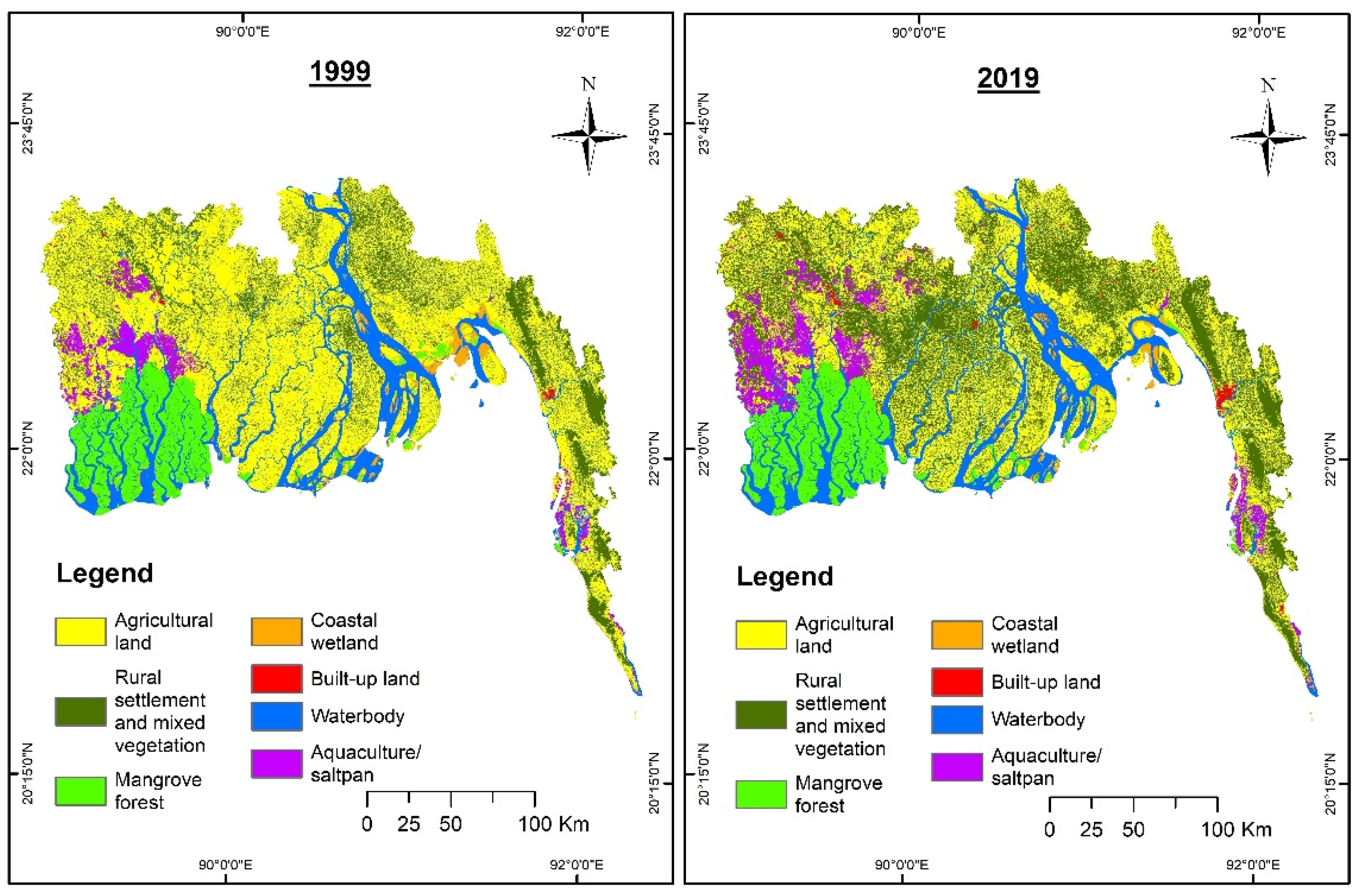
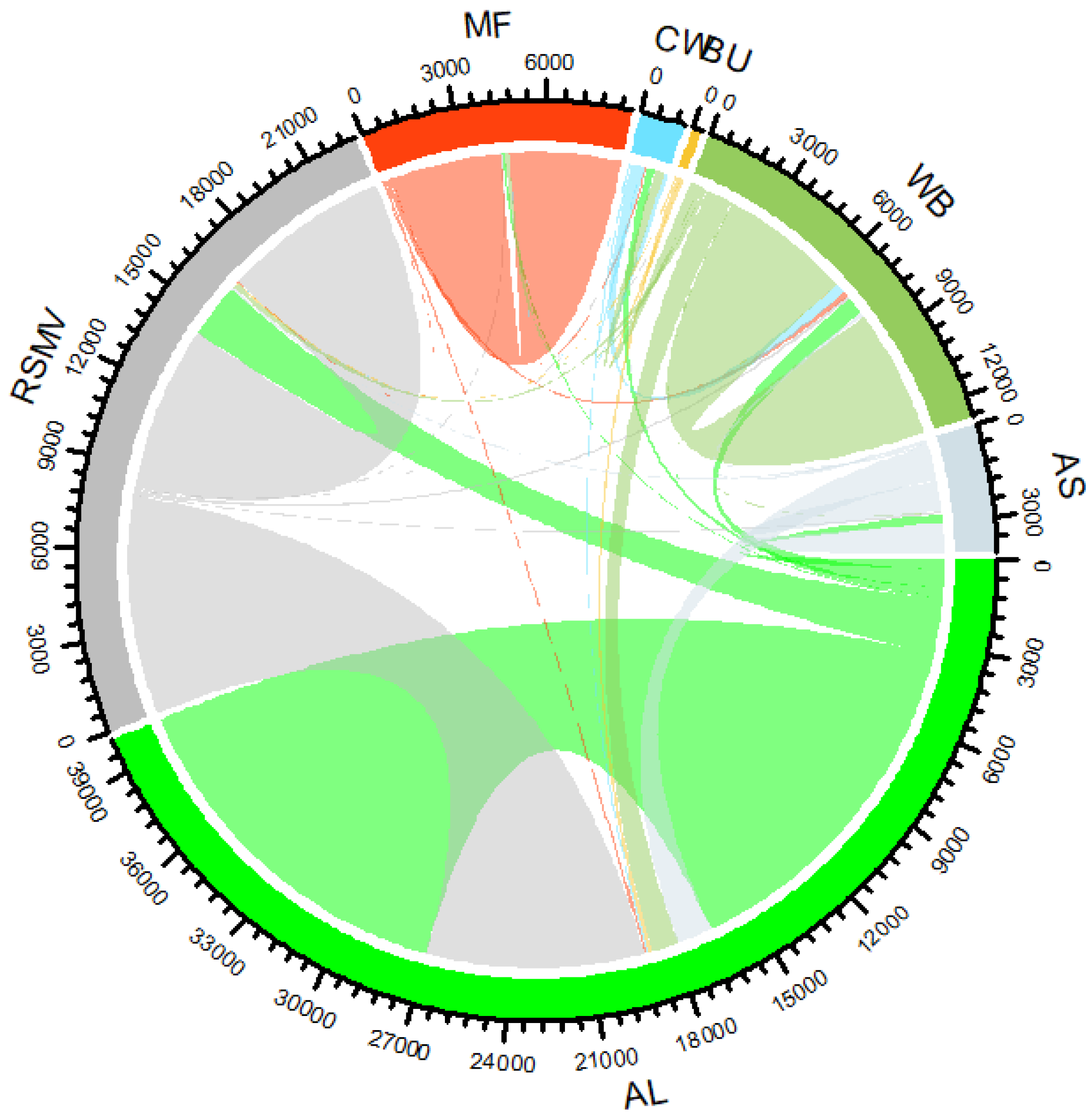
3.1. Dynamics of LULC Change during 1999–2019

Geographical distribution of coastal Bangladesh’s LULC patterns (Figure 3 and Table S1) depicts that agricultural land was the primary LULC class in 1999, accounting for about 52.40% of the total area. The areas covered by RSMV, waterbodies, and mangrove forest lands are also significant, with relative ratios of 18.60%, 13.83%, and 9.69%, respectively. The other LULC types, on the other hand (coastal wetland, built-up land, and aquaculture land), account for just 5.47% of the total area.

Between 1999 and 2019, we observed a growth in RSMV, mangrove forests, built-up areas, waterbodies, and aquaculture land, while agricultural and coastal wetland declined (Table S1). We noticed a rapid expansion in the built-up area over this time, at a rate of 15.38 percent per year, resulting in a total growth of 198.45 km². RSMV land increased at a 3.50 percent annual rate over the research period, totaling 5876.23 km², which is 2397.36 km² bigger than the combined aquaculture, coastal wetland, and built-up land area in 2019. Annual increases in aquaculture, waterbodies, and mangrove land were 3.49%, 0.17%, and 0.03%, respectively. Agriculture land lost the most land (30.15% (7125.69 km²)) between 1999 and 2019, while coastal wetland lost 30.02% (259.89 km²).

Additionally, we observed regional disparities in the geographical distribution of these important LULC types alterations (Table S2). During the study period, the highest loss of agricultural land was evident in Satkhira, Jhalokati, Pirojpur, Bagerhat, and Barisal district, with 57.28%, 57.26%, 55.37%, 48.09%, and 44.06%, respectively, from the base of year 1999, while Bhola and Chandpur districts had the lowest loss, 2.66%, and 4.72%, respectively, although none of the districts had seen an increase in the agricultural land. RSMV land assisted by homestead construction substantially increased over time with a rapid increase in the districts of Jhalokati (303.05%), Patuakhali (272.59%), Barguna (189.62%), Pirojpur (176.02%), Barisal (147.5%), Bagerhat (136.5%), and Khulna (116.24%) during 1999–2019 (Table S2). There were no apparent changes in mangrove forest cover in the three major districts of Bagerhat, Khulna, and Satkhira, which hosted more than 90% of the total mangrove forest in Bangladesh. However, due to the government’s projects on plantation mangrove forests, the acreage of mangrove forest has increased in the districts of Barguna (by 19.91%), Bhola (by 23.42%), Cox’s Bazar (by 98.34%), Patuakhali (by 155.48%), Feni (by 762.7%), and Lakshmipur (by 404.7%). During the study period, most of the districts experienced losses of coastal wetland, except for some districts such as Barisal and Shariatpur, which increased coastal wetland by 519.30% and 180.41%, respectively, which may have corresponded to accretion in the riverine areas. Built-up land increased in all coastal districts, with a rapid shift in Bagerhat (32,787.5%), Narail (2077.9%), Gopalganj (1942.5%), and Shariatpur (1539.05%) districts. Waterbodies rapidly increased in Lakshmipur (30.63%), Gopalganj (29.96%), Shariatpur (24.84%), Noakhali (21.93%), and Barisal (19.94%) districts, which could have corresponded to land erosion, while Cox’s Bazar showed the highest loss (34.07%) of waterbodies, which could have corresponded to the accretion process. Aquaculture land rose rapidly in the districts of Bagerhat (77.7%), Cox’s Bazar (48.7%), Khulna (12.1%), and Satkhira (119.5%), and these four districts constitute 87.34% of the total aquaculture/saltpan areas in 2019.

According to the chord diagram (Figure 4), the transfer amount of agricultural land, RSMV, wetlands, and waterbodies was rather significant. Between 1999 and 2019, 7940.7 km² of agricultural land was converted to RSMV, 1282 km² to aquaculture/saltpan, 986.7 km² to waterbodies, and 136 km² to built-up. From RSMV, 2001.5 km² was transformed into agricultural land, 170.4 km² into waterbodies, and 78 km² into aquaculture/saltpans. From coastal wetlands, 353.8 km² was converted to waterbodies and 280.4 km² to agricultural land. From waterbodies, 672.5 km² was converted to agricultural land, while the additional 386.7 km² was converted to wetlands. Besides, 329.8 km² of aquaculture/saltpan area was converted to agricultural land, whereas 67.6 km² of the same was converted to RSMV (Table S3). In general, the area of agricultural land converted to RSMV was greater than the area of RSMV converted to agricultural land, resulting in an increase in tree vegetation and a loss in agricultural land. Simultaneously, changes in the waterbodies were mostly transferred from agricultural land and coastal wetlands owing to fast riverbank erosion, while the accretion process resulted in a considerable rise in agricultural land and coastal wetlands.

3.2. Changes of ESV between 1999 and 2019

3.2.1. Change in Total ESV

The total ESV of CRB in 1999 was estimated at USD 25.18 billion (

Table 4. ESV and their change rate by different land use type in CRB between 1999 and 2019.

Component	AL	RSMV	MF	CW	BU	WB	AS	Total
ESV 1999 (109 USD)	10.73	3.74	5.18	0.59	0.00	4.77	0.17	25.18
ESV 1999 (%)	42.59	14.86	20.57	2.36	0.01	18.94	0.67	100
ESV 2019 (109 USD)	7.49	6.36	5.21	0.42	0.01	4.93	0.29	24.71
ESV 2019 (%)	30.31	25.75	21.09	1.68	0.05	19.96	1.15	100
ESV change 1999–2019 (109 USD)	−3.23	2.62	0.03	−0.179	0.01	0.16	0.12	−0.47
ESV change 1999–2019 (%)	−30.15	70.04	0.61	−30.02	307.56	3.39	69.74	−1.87

). Among the different land biomes, agricultural land contributed the highest of this value (about 42.59%), while it also occupied the highest portion (52.40%) of the whole landscape. Besides, mangrove forests, waterbodies, and RSMV contributed 20.57%, 18.94%, and 14.85%, respectively. Coastal wetlands accounted for 2.36%, while aquaculture/saltpan and built-up land contributed 0.66% and 0.01% of the total ESV of the study area, respectively.

Over the last two decades, the ESV of natural habitats (i.e., mangrove forest, RSMV, and water bodies) increased by USD 2.81 billion, from USD 13.70 billion in 1999 to USD 16.51 billion in 2019 (Table 4). The total ESV increase by these natural landscapes was largely contributed by the protection of natural mangrove forests, development of plantation mangroves, and planting of different tree species in and around rural homesteads and other settlement areas. In comparison, the total ESV of manmade ecosystems (i.e., built-up land and land used for aquaculture/saltpans) increased by USD 0.13 billion. However, the greatest loss of ESV was evident in agricultural land, which decreased by USD 3.23 billion (−30.15%), from USD 10.73 billion in 1999 to USD 7.49 billion in 2019. The ESV of coastal wetland decreased by USD 0.18 billion. Generally, the total ESV (between 1999 and 2019) in CRB plummeted by USD 0.47 billion, or reduced by 0.09 percent each year.

Figure 5 shows the contribution of each ecosystem function to the total ESVs, as well as a comparison of their contributions. Except for climate regulation (0.07%), water regulation (1.08%), and biodiversity protection (2.22%), all ecosystem service functions showed a decline from 1999 to 2019. The ESV for food production (−10.74%), raw materials (−7.75%), and waste treatment (−2.57%) suffered the most losses over the study period. Extreme event management (−0.24%), soil formation and retention (−1.17%), and recreational and cultural tourism (−1.66%) had the smallest ESV changes.

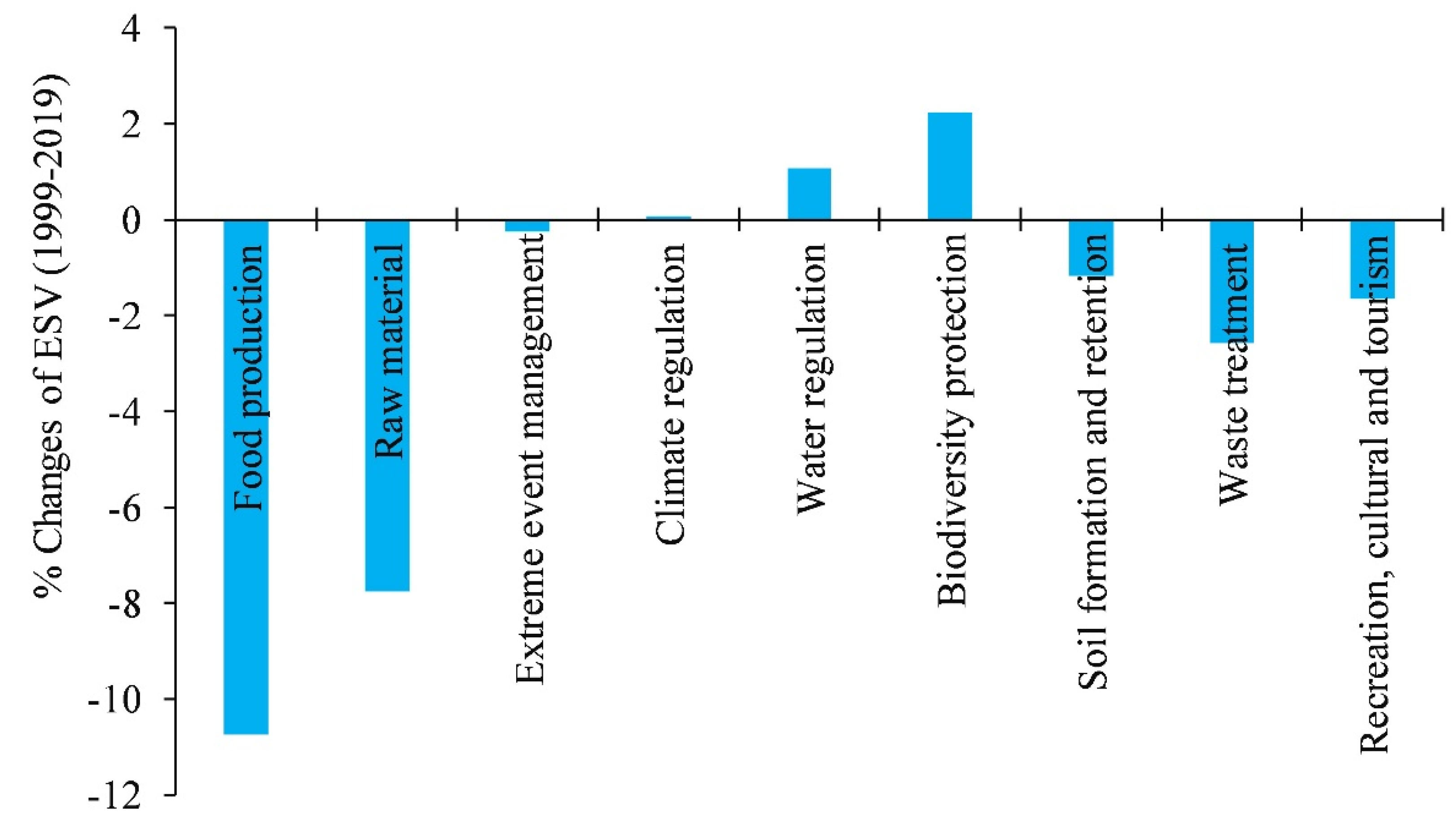
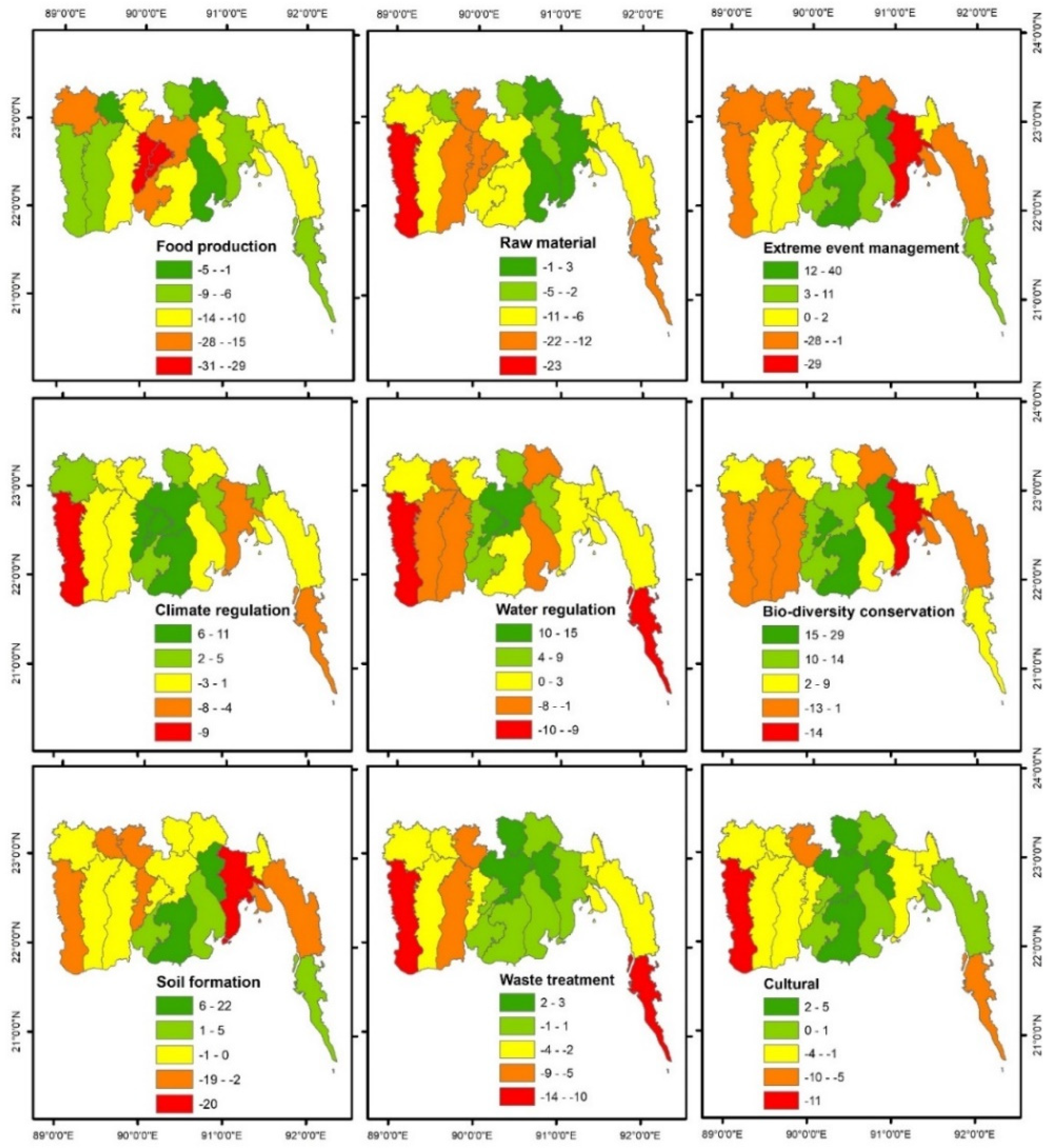
3.2.2. Spatial Variation in ESV Changes under Different Ecosystem Service Functions

The pattern of changes in the value of ecosystem service functions at the district scale is shown in Figure 6. The spatial distribution of ESV due to food production change revealed that the food production services decreased in all coastal districts, with the highest decrease in the districts of Jhalokati (−31.35%), Pirojpur (−29.11%), and Barisal (−20.67%). In the case of raw material production, the highest decrease was evident in the districts of Satkhira (−22.97%), Bagerhat (−15.50%), and Jahlokati (−15–25%), while only Noakhali district reported an increase in raw material by 3.11% during 1999–2019. The highest level of extreme event management capacity increased by 39.54%, 39.25%, and 11.25% in Lakshmipur, Patuakhali, and Cox’s Bazar districts, respectively, whereas the highest decrease was found in Noakahli (−29.29%) district. The climate regulation function value increased in 11 out of 19 districts, with the highest increase found in the districts Jhalokathi (10.86%), Patuakhali (6.97%), Barisal (6.43%), and Pirojpur (6.28%), whereas the highest decrease was found in Satkhira district (−9.22%). The increase in water regulation function value was highest in the districts Jhalokati (14.64%), and Barisal (10.60%), whereas the highest decrease was found in Cox’s Bazar (−8.68%) and Satkhira (−9.77%) districts. The biodiversity protection function value increased in all districts except Chandpur (−0.04%), Noakhali (−13.75%), and Satkhira (−2.94%), with the highest increase in Patuakhali (29.09%), Jhalokati (20.84%), and Lakshmipur (20.17%) districts. The increase in soil formation and retention function value was evident in Patuakhali (22.28%) and Lakshmipur (16.01%) districts, whereas the maximum decrease was found in Noakhali district (−19.51%). The highest decrease in waste treatment function value was found in the districts Satkhira (−13.79%), Cox’s Bazar (−9.94%), and Bagerhat (−5.91%), whereas the maximum increase was found in Shariatpur (3.16%) district. In terms of cultural and recreation function value, the highest decrease was reported in the districts Satkhira (−10.50%) and Cox’s Bazar (−6.51%), whereas the highest increase was found in Lakshmipur district (4.75%).

3.3. Spatial Autocorrelation of ESV in CRB

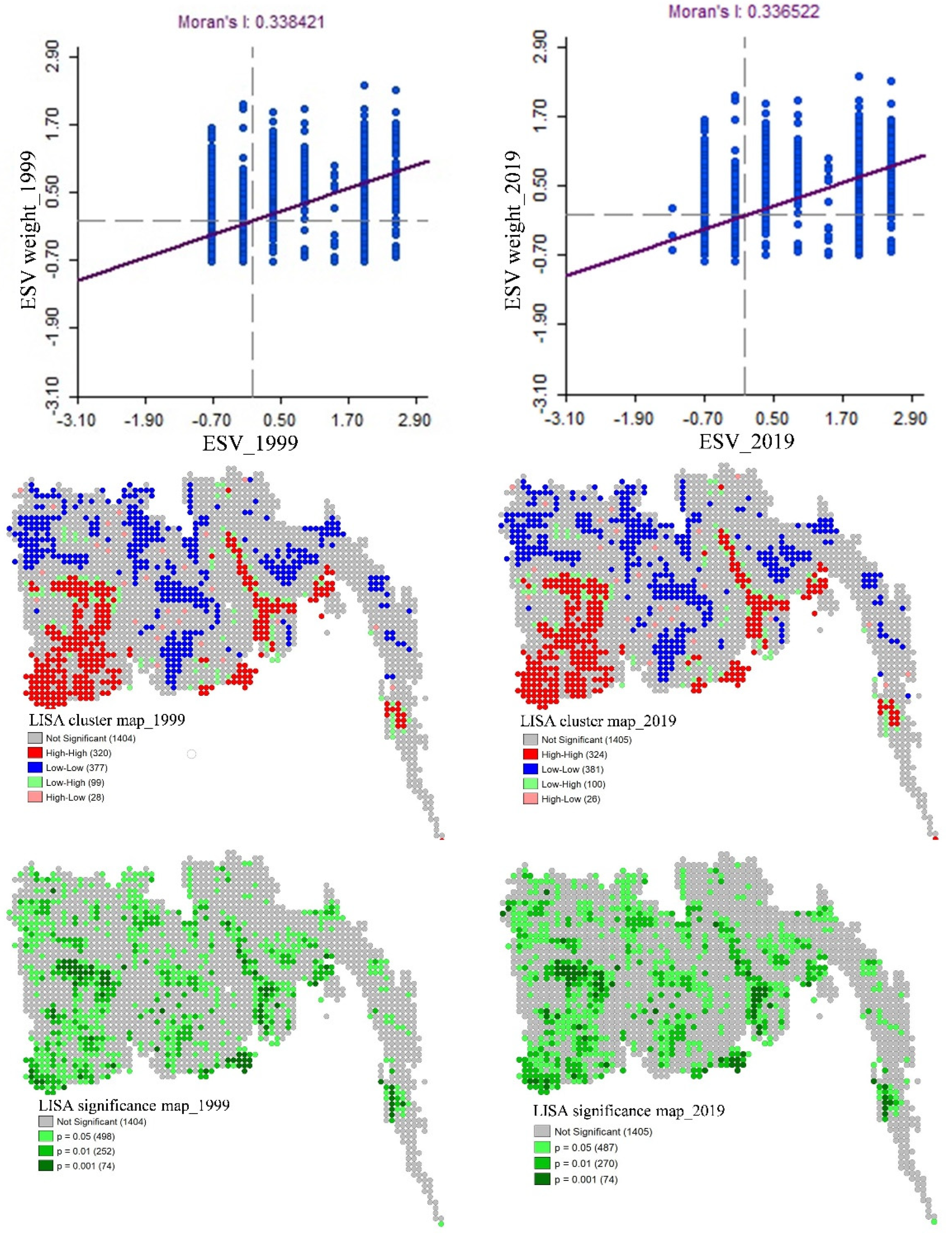
3.3.1. Global Spatial Autocorrelation of ESV

For 1999 and 2019, Moran scatter plots were obtained (Figure 7). The Moran’s I of the ESV is shown in Figure 7 for each time, with varying patterns. Moran’s I was 0.338421 and 0.336522 in 1999 and 2019, respectively, which were unusually high levels. The findings demonstrate that the ESV distribution pattern in the studied region was clearly clustered, indicating a significant positive connection. Between 1999 and 2019, the ESV’s Moran’s I decreased somewhat, indicating that the cluster phenomena of the ESV’s spatial distribution in this research region waned.

3.3.2. Local Spatial Autocorrelation of ESV

Only four kinds of significant autocorrelations can be detected in the research region: high-high (HH), low-low (LL), low-ligh (LH), and high-low (HL) (Figure 7). The local Moran’s I of the ESV had minor revisions from 1999 to 2019. Figure 7 reveals that the Sundarbans mangrove forest region and the broader GBM had the highest HH values (Ganges, Brahmaputra, and Meghna river areas). On the central coast, LL values were mostly found in inner coastal districts such as Jessore, Gopalganj, Barishal, and Narail, as well as the exposed coastal districts with bigger farmlands, such as Barguna, Patuakhali, Lakshmipur, and Noakali. The HL values were close to those of the LL area, indicating that this research region was in the transitional zone between landscape types. HL steadily rose in value. The geographical distribution of HH, LL, and HL regions might be intuitively represented by the LISA clustering map. The ESV significance level is reflected in the LISA significance map (Figure 7). The ESV’s significance threshold in LL and HH was 0.05, with some values at 0.01 and 0.001 as well. The ESV of these locations was connected to the ESV of nearby areas in a favorable way. In mangrove forests, waterbodies, and wetlands, the significant level was 0.01; this indicated that the spatial distribution of ESV was highly converging and exhibited a strong association. Between 1999 and 2019, the area of the significant region (p = 0.05) declined, while the extent of the more significant region (p = 0.01) rose, and the highest significant region (p = 0.001) stayed steady.

3.4. Sensitivity of Ecosystem Services

Table 5. Total approximate ecosystem services and coefficient of sensitivity (CS) in CRB after changing the ES valuation coefficient (VC) from 1999 to 2019.

Change in Value Coefficient	1999		2019
	Percent	CS	Percent	CS
Agriculture ± 50%	±21.294	0.426	±15.157	0.303
RSMV ± 50%	±7.429	0.149	±12.873	0.257
Mangrove forest ± 50%	±10.285	0.206	±10.546	0.211
Coastal wetland ± 50%	±1.181	0.024	±0.842	0.017
Built-up ± 50%	±0.006	0.000	±0.025	0.000
Water body ± 50%	±9.471	0.189	±9.979	0.200
Aquaculture/salt ± 50%	±0.334	0.007	±0.577	0.012

shows the results of using alternate value coefficients to measure the cumulative value of ES over two years. In all years, the estimated CS for all land use groups was less than unity, indicating that the estimated cumulative ecosystem service values for the sample area are somewhat inelastic in terms of the value coefficients. For coastal wetlands, built-up, aquaculture, and others, the CS ranged from 0.000 to 0.024. When the valuation coefficient for these land use divisions was changed by 50%, the CS varied from 0.000–0.000 for built-up to 0.303–0.426 for agriculture. This finding also suggested that the estimates of ecosystem service values are reliable where strongly undervalued or overvalued coefficients can have a significant impact on the degree to which estimates of ecosystem service values change over time.

4. Discussion

4.1. Land Use Land Cover Change and Associated Ecosystem Service Value Change

The most common LULC change in Bangladesh’s coastal area was the loss of cultivated land to rural settlement building, followed by rural settlement-based vegetation development, which was also validated in previous research [25,36]. We calculated that the overall ESV in the study area declined by 1.87% (USD 0.47 billion) from 1999 to 2019 based on the approximate size of the seven LULC categories and our ecosystem service assessment methodology. The transfer of a significant quantity of agricultural land to the development of rural communities and urban built-up regions was mainly attributed to the loss of ESVs. The reduction of coastal wetlands also made a substantial contribution to the overall loss of ESVs. However, the development of various vegetation resources surrounding the rural community resulted in a significant improvement in ESs, which more than compensated for the loss of ecosystem services as a result of agricultural land loss. Furthermore, the growth of coastal afforestation via planting mangrove species has helped to reduce total ESV losses in CRB. Positive change was apparent at the district level owing to the growth of RSMV in the northern and eastern districts, while the development of plantation mangrove forests in the south-central and southwestern districts increased the ESV. The drop in ESV in certain districts, such as Cox’s Bazar, was primarily caused by the loss of inland agricultural areas and mountainous forest vegetation owing to settlement building to house over a million refugees who fled Myanmar as a consequence of the Myanmar government’s ethnic cleansing of the Rohingya people [46].

In contrast to our findings, research in other parts of the globe documenting agricultural land expansion and associated ESV assessment methods has shown a decrease in total ESV [44,45,47]. One of the most important elements in preventing the overall ESV change due to agricultural land losses has been the government’s progressive effort to enhance the vegetation by planting various fruit, fuelwood, and forest species in and surrounding rural settlements, as well as the coastal greenbelt project for mangrove plantation [48,49,50,51,52]. Moreover, among the many other variables, variance in the value coefficients employed may be to blame. This (previous) research utilized Costanza et al. [2] valuation coefficients, which differ significantly from Costanza et al. [34] coefficients, partly due to the high number of case studies used in 2014 to get the values for each land biome [53]. If we look at how much ecosystem service value has been lost in CRB over the last two decades based on locally estimated value coefficient, we can see that maintaining the important ecosystem services is a significant problem that may be somewhat offset by ecosystem-based land use planning, such as planting trees of various types in and around the settlement area. The biggest compensation for the general decline in the significance of natural ecosystem service in Bangladesh’s coastal area is forest restoration and RSMV development in many locations. This corresponds to the findings of [25], who found that forest planting in the central CRB contributed the most in raising the ecological service value.

The shift from agriculture to other land uses has resulted in a reduction in food and raw material output in the coastal area, which is contrary to the worldwide trend of agricultural growth. The underlying reason of this may be Bangladesh’s ever-increasing population, which necessitates massive homestead construction and urban landscape development [25]. In addition, the substantial reduction in many ES functions has major policy implications for balancing food security and ecological services. This is similar to the results of many previous research, which showed the supply of various ecosystem services such as food production [25,26,36], raw material [25,27,36,54], waste treatment [55], and soil formation [36]. The impact of improving services such as climate and water management, as well as biological conservation, is already seen in the coastal region of Bangladesh for implementing various ecosystem-based adaptation methods [28,56,57].

In CRB, HH and LL showed positive correlations with ESV. HL and LH outliers also developed sporadically in various regions. High-density clusters were found in primary tropical rainforest, natural and plantation mangroves, and close to water (rivers and wetlands); this might be explained by the rich biodiversity, material exchanges, and energy conversion of aquatic ecosystems. Meanwhile, LL clusters were discovered close to communities and nearby farmlands, as well as in long-established protected zones. Urban and agricultural development, as well as other human activities, usually damage these places, affecting the natural ecosystem functions and lowering their ESV. Therefore, by being aware of the geographical distribution of ESV, conservation managers may better successfully manage resources. The degree of land use might be reduced by efficiently reestablishing vegetation on unused and dry areas, thereby boosting biodiversity, ESV, and ecological integrity in the CRB. Managers could protect the slopes for afforestation or ecological restoration. Strict restrictions on urbanization may encourage compact human settlements, which would protect the environment by lowering carbon emissions and environmental disruptions.

4.2. Challenges of Sustainability of Land Management and Ways Forward

Apart from the anthropogenic factors such as high population growth and increased economic activity, the geographical position of Bangladesh makes the LULC pattern of coastal regions sensitive to several climatic shocks and stresses, which in turn creates a significant challenge for achieving land use sustainability. For instance, increased temperature, erratic rainfall, and sea-level rise induced saline water intrusion in agricultural lands (Figure 8). Meanwhile, almost 63% of arable land in the coastal zone has been impacted by varying levels of soil salinity [58] and is expected to be elevated further in the current century due to SLR. It is also estimated that a one-meter rise in sea level could submerge about 20% of the total landmass of Bangladesh, displacing 20–30 million people from the coastal zone [59,60].

The agricultural development in this region is primarily constrained by poor soil fertility, heavy soil texture, soil salinity in the dry season (Figure 8), and poor polder management [61,62]. These constraints affect both cropping intensity and production, which instigate the coastal people to switch over to alternate land use such as shrimp culture or salt farms from traditional crop-based farming practices by building embankments [63]. Shrimp farming increased very rapidly, from 2000 ha in 1970 to 275,000 ha in 2013, due to the motivation of higher profitability, international demand, and interest from government, development agencies, and private entrepreneurs [64,65]. Allowing the entry of saltwater for shrimp culture has reduced the cultivated land and created new lands under saline water, especially when embankments are damaged, causing land degradation and environmental problems [66]. During the monsoon season, there are floods almost every year, with multiple events that lead to a large area of land erosion and accretion, which destroy human well-being, settlement areas, and agricultural land and render dwellers landless, putting their livelihoods at risk. Over the different time horizons, the increased frequency and intensity of different climatic hazards (Figure 8) has directed rapid LULC change in this region, destroying the biodiversity of coastal ecosystems, creating unemployment, reducing agricultural production, and escalating food and livelihood insecurity of the coastal community.

With the loss of natural habitats and their associated resources, some of the limitations in the agricultural sector will increase and therefore further jeopardize agricultural output. A further reduction in the forest clearing (climate protection service) will accelerate global warming, a significant ecosystem challenge that would also impact productivity in the agriculture sector among many other implications. For instance, crop yields are predicted to decrease by 10–20 percent or 50 percent by 2050 due to climatic variation/ change [70]. This is no exception to the coastal area of Bangladesh, an extremely climatically prone country with a poor adaptive potential that depends on the natural resources for agriculture [28,69]. Considering the extreme susceptibility of CRB to global climate change-induced natural disasters such as cyclones, rising sea levels, salinity, erosion, and flooding [28,62,69,71,72], we advocate that the conservation of cultivated land should take precedence in the future.

The CRB should be prioritized for developing ecosystem-based adaptation such as the protection of wetlands and forest lands as well as the development of mangrove plantations [73]. As a hard measure, the construction of dams and frequent dredging of the river channels should be done to protect the erosion [57]. Another important adaptation could be the development of more saline-resistant crop varieties, which should be adapted to saline-prone croplands (consequence of sea-level rise) [28,69]. Upon discussion, the government of Bangladesh may also initiate a crop insurance policy for agricultural farmers to ensure compensation when a disaster event causes loss to their farm products [57,74,75].

4.3. Limitations of the Study

The research has several limitations that will need to be resolved in future studies. To begin, we analyzed the LULC patterns using open-source Landsat imagery and a supervised classification algorithm, which may result in some misclassification due to the difficulty of the LULC pattern in Bangladesh at a local scale [25]. This was enhanced, however, by using the Semi-automated Classification Plugin’s post-processing feature, as well as ground-truthing, field visits, literature reviews, and Google Earth image archives and editing the misclassification. Furthermore, we did not take into account any particular biophysical considerations for sensitivity analysis, which may be achieved in future studies [76]. Finally, the ESV assessment used in the study could have overestimated or underestimated the real importance of Bangladesh’s coastal land biomes, which could be corrected by performing national-level estimations of ecosystem service values in different land biomes by an eminent expert panel of government.

5. Conclusions

The land use land cover of coastal Bangladesh has dramatically altered between 1999 and 2019. The most apparent transformation was evident between agricultural land and rural settlement-based vegetation. Between 1999 and 2019, the total ESVs of CRB decreased by 1.87%, from USD 25.18 × 10⁹ in 1999 to USD 24.71 × 10⁹ in 2019, owing to decreasing agricultural land and wetlands, as well as the expansion of settlements and aquaculture/saltpans. Among the different ESs, values of food and raw materials declined, while values of biodiversity conservation and water management increased notably. The spatial variation of ESV was prominent. It was found that districts with mangroves possessed an exceptionally high total ESV, such as Satkhira, Khulna, and Bagerhat. A significant spatial correlation and moderately high spatial clustering were observed, which consisted mostly in mangrove forests, waterbodies, and wetland zones. Both high-high and low-low values increased, but spatial outliers remained almost unchanged. In coastal Bangladesh, the sustainability of land use management in the face of potential anthropogenic causes and adverse climate change scenarios requires striking a balance between the conservation of natural resources and the preservation of cultivable agricultural land. The results of this research concerning growing mangroves and RSMV development have important policy implications for constructing a barrier against ESV loss caused by a significant decrease in agricultural areas in other regions of the globe, as well as associated socio-geographical and environmental issues.

References

1. Costanza, R.; Cumberland, J.H.; Daly, H.; Goodland, R.; Norgaard, R.B. An Introduction to Ecological Economics; CRC Press: Boca Raton, FL, USA, 1997. [Google Scholar]
2. Costanza, R.; D’Arge, R.; De Groot, R.; Farber, S.; Grasso, M.; Hannon, B.; Limburg, K.; Naeem, S.; O’Neill, R.V.; Paruelo, J.; et al. The value of the world’s ecosystem services and natural capital. Nature 1997, 387, 253–260. [Google Scholar] [CrossRef]
3. Daily, G.C. Nature’s Services: Societal Dependence on Natural Ecosystems; Yale University Press: New Haven, CT, USA, 1997. [Google Scholar]
4. Feng, X.Y.; Luo, G.P.; Li, C.F.; Dai, L.; Lu, L. Dynamics of ecosystem service value caused by land use changes in Manas River of Xinjiang, China. Int. J. Environ. Res. 2012, 6, 499–508. [Google Scholar]
5. Zhan, J. Impacts of Land-Use Change on Ecosystem Services; Springer: Berlin/Heidelberg, Germany, 2015. [Google Scholar]
6. Arowolo, A.O.; Deng, X.; Olatunji, O.A.; Obayelu, A.E. Assessing changes in the value of ecosystem services in response to land-use/land-cover dynamics in Nigeria. Sci. Total Environ. 2018, 636, 597–609. [Google Scholar] [CrossRef] [PubMed]
7. Arowolo, A.O.; Deng, X. Land use/land cover change and statistical modelling of cultivated land change drivers in Nigeria. Reg. Environ. Change 2018, 18, 247–259. [Google Scholar] [CrossRef]
8. Ellis, E.; Pontius, R. Land-use and land-cover change. Encycl. Earth 2007, 1, 1–4. [Google Scholar]
9. Giri, C.P. Remote Sensing of Land Use and Land Cover: Principles and Applications; CRC press: Boca Raton, FL, USA, 2012. [Google Scholar]
10. MEA. Ecosystems and Human Well-Being: Synthesis; A Report of the Millennium Ecosystem Assessment; Island Press: Washington, DC, USA, 2005. [Google Scholar]
11. De Araujo Barbosa, C.C.; Atkinson, P.M.; Dearing, J.A. Remote sensing of ecosystem services: A systematic review. Ecol. Indic. 2015, 52, 430–443. [Google Scholar] [CrossRef]
12. Feng, X.; Fu, B.; Yang, X.; Lü, Y. Remote sensing of ecosystem services: An opportunity for spatially explicit assessment. Chin. Geogr. Sci. 2010, 20, 522–535. [Google Scholar] [CrossRef] [Green Version]
13. O’Neil-Dunne, J.; MacFaden, S.; Royar, A. A versatile, production-oriented approach to high-resolution tree-canopy mapping in urban and suburban landscapes using GEOBIA and data fusion. Remote Sens. 2014, 6, 12837–12865. [Google Scholar] [CrossRef] [Green Version]
14. Zheng, G.; Moskal, L.M. Retrieving leaf area index (LAI) using remote sensing: Theories, methods and sensors. Sensors 2009, 9, 2719–2745. [Google Scholar] [CrossRef] [Green Version]
15. Zhu, Z.; Fu, Y.; Woodcock, C.E.; Olofsson, P.; Vogelmann, J.E.; Holden, C.; Wang, M.; Dai, S.; Yu, Y. Including land cover change in analysis of greenness trends using all available Landsat 5, 7, and 8 images: A case study from Guangzhou, China (2000–2014). Remote Sens. Environ. 2016, 185, 243–257. [Google Scholar] [CrossRef] [Green Version]
16. De Beurs, K.M.; Henebry, G.M. Land surface phenology, climatic variation, and institutional change: Analyzing agricultural land cover change in Kazakhstan. Remote Sens. Environ. 2004, 89, 497–509. [Google Scholar] [CrossRef]
17. Andrew, M.E.; Wulder, M.A.; Nelson, T.A. Potential contributions of remote sensing to ecosystem service assessments. Prog. Phys. Geogr. 2014, 38, 328–353. [Google Scholar] [CrossRef] [Green Version]
18. Morgan Grove, J.; Cadenasso, M.L.; Burch Jr, W.R.; Pickett, S.T.A.; Schwarz, K.; O’Neil-Dunne, J.; Wilson, M.; Troy, A.; Boone, C. Data and methods comparing social structure and vegetation structure of urban neighborhoods in Baltimore, Maryland. Soc. Nat. Resour. 2006, 19, 117–136. [Google Scholar] [CrossRef]
19. Pandey, P.C.; Balzter, H.; Srivastava, P.K.; Petropoulos, G.P.; Bhattacharya, B. Future perspectives and challenges in hyperspectral remote sensing. Hyperspectral Remote Sens. 2020, 429–439. [Google Scholar] [CrossRef]
20. Cortinovis, C.; Geneletti, D.; Hedlund, K. Synthesizing multiple ecosystem service assessments for urban planning: A review of approaches, and recommendations. Landsc. Urban Plan. 2021, 213, 104129. [Google Scholar] [CrossRef]
21. Bryan, B.A.; Crossman, N.D. Impact of multiple interacting financial incentives on land use change and the supply of ecosystem services. Ecosyst. Serv. 2013, 4, 60–72. [Google Scholar] [CrossRef]
22. Bryan, B.A.; Crossman, N.D.; Nolan, M.; Li, J.; Navarro, J.; Connor, J.D. Land use efficiency: Anticipating future demand for land-sector greenhouse gas emissions abatement and managing trade-offs with agriculture, water, and biodiversity. Glob. Chang. Biol. 2015, 21, 4098–4114. [Google Scholar] [CrossRef]
23. Ye, Y.; Bryan, B.A.; Zhang, J.; Connor, J.D.; Chen, L.; Qin, Z.; He, M. Changes in land-use and ecosystem services in the Guangzhou-Foshan Metropolitan Area, China from 1990 to 2010: Implications for sustainability under rapid urbanization. Ecol. Indic. 2018, 93, 930–941. [Google Scholar] [CrossRef]
24. Liu, J.; Dietz, T.; Carpenter, S.R.; Alberti, M.; Folke, C.; Moran, E.; Pell, A.N.; Deadman, P.; Kratz, T.; Lubchenco, J.; et al. Complexity of coupled human and natural systems. Science 2007, 317, 1513–1516. [Google Scholar] [CrossRef] [Green Version]
25. Hoque, M.Z.; Cui, S.; Islam, I.; Xu, L.; Tang, J. Future impact of land use/land cover changes on ecosystem services in the lower meghna river estuary, Bangladesh. Sustainability 2020, 12, 2112. [Google Scholar] [CrossRef] [Green Version]
26. Hoque, M.Z.; Cui, S.; Islam, I.; Xu, L.; Ding, S. Dynamics of plantation forest development and ecosystem carbon storage change in coastal Bangladesh. Ecol. Indic. 2021, 130, 107954. [Google Scholar] [CrossRef]
27. Huq, N.; Bruns, A.; Ribbe, L. Interactions between freshwater ecosystem services and land cover changes in southern Bangladesh: A perspective from short-term (seasonal) and long-term (1973–2014) scale. Sci. Total Environ. 2019, 650, 132–143. [Google Scholar] [CrossRef] [PubMed]
28. Hoque, M.Z.; Cui, S.; Xu, L.; Islam, I.; Tang, J.; Ding, S. Assessing agricultural livelihood vulnerability to climate change in coastal Bangladesh. Int. J. Environ. Res. Public Health 2019, 16, 4552. [Google Scholar] [CrossRef] [PubMed] [Green Version]
29. World Economic Forum Here’s what You Need to Know about Bangladesh’s Rocketing Economy. Available online: https://www.weforum.org/agenda/2019/11/bangladesh-gdp-economy-asia/ (accessed on 24 February 2020).
30. BBS. Population and Housing Census 2011; Bangladesh Bureau of Statistics; Ministry of Planning, Government of the Peoples’ Republic of Bangladesh: Dhaka, Bangladesh, 2011.
31. Thomas, M.B.; Wratten, S.D.; Nick, S. Creation of island habitats densities predator arthropods: Of beneficial populations and species composition. J. App. Ecol. 1992, 29, 524–531. [Google Scholar] [CrossRef]
32. Iftekhar, M.S. Conservation and management of the Bangladesh coastal ecosystem: Overview of an integrated approach. Nat. Resour. Forum. 2006, 30, 230–237. [Google Scholar] [CrossRef]
33. MoWR. Integrated Coastal Zone Management: Concepts and Issues; A Government of Bangladesh Policy: Dhaka, Bangladesh, 1999.
34. Costanza, R.; De Groot, R.; Sutton, P.; Van Der Ploeg, S.; Anderson, S.J.; Kubiszewski, I.; Farber, S.; Turner, R.K. Changes in the global value of ecosystem services. Glob. Environ. Change 2014, 26, 152–158. [Google Scholar] [CrossRef]
35. Congedo, L. Semi-Automatic Classification Plugin: A Python tool for the download and processing of remote sensing images in QGIS. J. Open Source Softw. 2021, 6, 3172. [Google Scholar] [CrossRef]
36. Akber, M.A.; Khan, M.W.R.; Islam, M.A.; Rahman, M.M.; Rahman, M.R. Impact of land use change on ecosystem services of southwest coastal Bangladesh. J. Land Use Sci. 2018, 13, 238–250. [Google Scholar] [CrossRef]
37. Dibaba, W.T.; Demissie, T.A.; Miegel, K. Drivers and Implications of Land Use/Land Cover Dynamics in Finchaa Catchment, Northwestern Ethiopia. Land 2020, 9, 113. [Google Scholar] [CrossRef] [Green Version]
38. Chow, J. Spatially Explicit Evaluation of Local Extractive Benefits from Mangrove Plantations in Bangladesh. J. Sustain. For. 2015, 34, 651–681. [Google Scholar] [CrossRef]
39. Ullah, M.H.; Mondal, M.A.I.; Uddin, M.R.; Ferdous, M.A. Implications of Mangrove Wetland in Socio-environmental Sector: Experiences from Southeast Coast of Chittagong, Bangladesh. J. For. Environ. Sci. 2010, 26, 103–111. [Google Scholar]
40. Zhang, F.; Yushanjiang, A.; Jing, Y. Assessing and predicting changes of the ecosystem service values based on land use/cover change in Ebinur Lake Wetland National Nature Reserve, Xinjiang, China. Sci. Total Environ. 2019, 656, 1133–1144. [Google Scholar] [CrossRef] [PubMed]
41. Mansfield, C.Y. Elasticity and buoyancy of a tax system: A method applied to Paraguay. Staff Pap. 1972, 19, 425–446. [Google Scholar] [CrossRef]
42. Kreuter, U.P.; Harris, H.G.; Matlock, M.D.; Lacey, R.E. Change in Ecosystem Service Values in the San Antonio Area, Texas. Ecol. Econ. 2001, 39, 333–346. [Google Scholar] [CrossRef]
43. Gashaw, T.; Tulu, T.; Argaw, M.; Worqlul, A.W.; Tolessa, T.; Kindu, M. Estimating the impacts of land use/land cover changes on Ecosystem Service Values: The case of the Andassa watershed in the Upper Blue Nile basin of Ethiopia. Ecosyst. Serv. 2018, 31, 219–229. [Google Scholar] [CrossRef]
44. Li, R.-Q.; Dong, M.; Cui, J.-Y.; Zhang, L.-L.; Cui, Q.-G.; He, W.-M. Quantification of the impact of land-use changes on ecosystem services: A case study in Pingbian County, China. Environ. Monit. Assess. 2007, 128, 503–510. [Google Scholar] [CrossRef]
45. Zhao, B.; Kreuter, U.; Li, B.; Ma, Z.; Chen, J.; Nakagoshi, N. An ecosystem service value assessment of land-use change on Chongming Island, China. Land Use Policy 2004, 21, 139–148. [Google Scholar] [CrossRef]
46. Rashid, K.J.; Hoque, M.A.; Esha, T.A.; Rahman, M.A.; Paul, A. Spatiotemporal changes of vegetation and land surface temperature in the refugee camps and its surrounding areas of Bangladesh after the Rohingya influx from Myanmar. Environ. Dev. Sustain. 2021, 23, 3562–3577. [Google Scholar] [CrossRef]
47. Wang, Z.; Zhang, B.; Zhang, S.; Li, X.; Liu, D.; Song, K.; Li, J.; Li, F.; Duan, H. Changes of land use and of ecosystem service values in Sanjiang Plain, Northeast China. Environ. Monit. Assess. 2006, 112, 69–91. [Google Scholar] [CrossRef]
48. Hocking, D.; Hocking, A.; Islam, K. Trees on farms in Bangladesh. Agrofor. Syst. 1996, 33, 231–247. [Google Scholar] [CrossRef]
49. Rahman, M.M.; Furukawa, Y.; Kawata, I.; Rahman, M.M.; Alam, M. Homestead forest resources and their role in household economy: A Case Study in the villages of Gazipur sadar upazila of central Bangladesh. Small-Scale For. Econ. Manag. Policy 2005, 4, 359–376. [Google Scholar] [CrossRef]
50. Miah, M.G.; Hussain, M.J. Homestead Agroforestry: A Potential Resource in Bangladesh. In Sociology, Organic Farming, Climate Change and Soil Science; Springer: Berlin/Heidelberg, Germany, 2010; pp. 437–463. [Google Scholar]
51. Saenger, P.; Siddiqi, N.A. Land from the sea: The mangrove afforestation program of Bangladesh. Ocean. Coast. Manag. 1993, 20, 23–39. [Google Scholar] [CrossRef] [Green Version]
52. Shamsuddoha, M.; Haque, M.I.M.A.; Rahman, M.F.; Roberts, E.; Hasemann, A.; Roddick, S. Local Perspective on Loss and Damage in the Context of Extreme Events: Insights from Cyclone-Affected Communities in Coastal Bangladesh; Centre for Participatory Research and Developement (CRPD): Dhaka, Bangladesh, 2013. [Google Scholar]
53. Yi, H.; Güneralp, B.; Filippi, A.M.; Kreuter, U.P.; Güneralp, İ. Impacts of Land Change on Ecosystem Services in the San Antonio River Basin, Texas, from 1984 to 2010. Ecol. Econ. 2017, 135, 125–135. [Google Scholar] [CrossRef]
54. Hoque, M.Z.; Islam, I.; Ahmed, M.; Hasan, S.S.; Prodhan, F.A. Spatio-temporal changes of land use land cover and ecosystem service values in coastal Bangladesh. Egypt. J. Remote Sens. Sp. Sci. 2022, 25, 173–180. [Google Scholar]
55. Hasan, S.; Shi, W.; Zhu, X. Impact of land use land cover changes on ecosystem service value—A case study of Guangdong, Hong Kong, and Macao in South China. PLoS ONE 2020, 15, e0231259. [Google Scholar] [CrossRef] [Green Version]
56. Hoque, M.Z.; Cui, S.; Lilai, X.; Islam, I.; Ali, G.; Tang, J. Resilience of coastal communities to climate change in Bangladesh: Research gaps and future directions. Watershed Ecol. Environ. 2019, 1, 42–56. [Google Scholar] [CrossRef]
57. Minar, M.H.; Hossain, M.B.; Shamsuddin, M.D. Climate change and coastal zone of Bangladesh: Vulnerability, resilience and adaptability. Middle East J. Sci. Res. 2013, 13, 114–120. [Google Scholar] [CrossRef]
58. SRDI. Saline Soils of Bangladesh; Soil Resource Development Institute (SRDI), Ministry of Agriculture, Government of the People’s Republic of Bangladesh: Dhaka, Bangladesh, 2010.
59. IPCC. Climate Change 2014: Impacts, Adaptation and Vulnerability—Contributions of the Working Group II to the Fifth Assessment Report; IPCC: Geneva, Switzerland, 2014. [Google Scholar]
60. MoEF. Bangladesh Climate Change Strategy and Action Plan 2009; Ministry of Environment and Forestry (MoEF), Government of the People’s Republic of Bangladesh: Dhaka, Bangladesh, 2009.
61. Haque, S.A. Salinity problems and crop production in coastal regions of Bangladesh. Pakistan J. Bot. 2006, 38, 1359–1365. [Google Scholar]
62. Chowdhury, A.K.M.H.U.; Haque, M.E.; Hoque, M.Z.; Rokonuzzam, M. Adoption of BRRI Dhan47 in the Coastal Saline areas of Bangladesh. Agric. J. 2012, 7, 286–291. [Google Scholar] [CrossRef]
63. Islam, M.R. Managing Diverse Land Uses in Coastal Bangladesh: Institutional Approaches. Environ. livelihoods Trop. Coast. Zo. 2006, 18, 237. [Google Scholar]
64. FRSS. Fisheries Statistical Year Book of Bangladesh 2013–2014; Fisheries Resource Survey System (FRSS), Ministry of Fisheries and Livestock, Government of the Peoples’ Republic of Bangladesh: Dhaka, Bangladesh, 2015.
65. Pokrant, B. Brackish Water Shrimp Farming and the Growth of Aquatic Monocultures in Coastal Bangladesh. In Historical Perspectives of Fisheries Exploitation in the Indo-Pacific; MARE Publication Series; Springer: Berlin/Heidelberg, Germany, 2014; p. 10732. [Google Scholar]
66. Islam, S.N. Deltaic floodplains development and wetland ecosystems management in the Ganges–Brahmaputra–Meghna Rivers Delta in Bangladesh. Sustain. Water Resour. Manag. 2016, 2, 237–256. [Google Scholar] [CrossRef] [Green Version]
67. BBS. Statistical Yearbook of Bangladesh 2018; Bangladesh Bureau of Statistics (BBS), Ministry of Planning, Government of the Peoples’ Republic of Bangladesh: Dhaka, Bangladesh, 2018.
68. Ahmed, A.; Drake, F.; Nawaz, R.; Woulds, C. Where is the coast? Monitoring coastal land dynamics in Bangladesh: An integrated management approach using GIS and remote sensing techniques. Ocean Coast. Manag. 2018, 151, 10–24. [Google Scholar] [CrossRef]
69. Hoque, M.Z.; Haque, E.; Islam, S. Mapping integrated vulnerability of coastal agricultural livelihood to climate change in Bangladesh: Implications for spatial adaptation planning. Phys. Chem. Earth Parts A/B/C 2021, 125, 103080. [Google Scholar] [CrossRef]
70. Jones, P.G.; Thornton, P.K. The potential impacts of climate change on maize production in Africa and Latin America in 2055. Glob. Environ. Change 2003, 13, 51–59. [Google Scholar] [CrossRef]
71. Kamruzzaman, M.; Rahman, A.T.M.S.; Ahmed, M.S.; Kabir, M.E.; Mazumder, Q.H.; Rahman, M.S.; Jahan, C.S. Spatio-temporal analysis of climatic variables in the western part of Bangladesh. Environ. Dev. Sustain. 2018, 20, 89–108. [Google Scholar] [CrossRef]
72. Prodhan, F.A.; Zhang, J.; Sharma, T.P.P.; Nanzad, L.; Zhang, D.; Seka, A.M.; Ahmed, N.; Hasan, S.S.; Hoque, M.Z.; Mohana, H.P. Projection of future drought and its impact on simulated crop yield over South Asia using ensemble machine learning approach. Sci. Total Environ. 2022, 807, 151029. [Google Scholar] [CrossRef]
73. Nicholls, R.J.; Hutton, C.W.; Adger, W.N.; Hanson, S.E.; Rahman, M.M.; Salehin, M. Ecosystem Services for Well-Being in Deltas; Springer International Publishing: Berlin/Heidelberg, Germany, 2018. [Google Scholar]
74. Abedin, M.A.; Shaw, R. Agriculture Adaptation in Coastal Zone of Bangladesh. In Climate Change Adaptation Actions in Bangladesh. Disaster Risk Reduction (Methods, Approaches and Practices); Shaw, R., Mallick, F., Islam, A., Eds.; Springer: Tokyo, Japan, 2013; pp. 207–226. [Google Scholar]
75. Ahmed, S.N.; Islam, A. Climate Change Adaptation Actions in Bangladesh; Disaster Risk Reduction; Springer: Berlin/Heidelberg, Germany, 2013; ISBN 978-4-431-54248-3. [Google Scholar]
76. Bourgin, M.; Labarthe, S.; Kriaa, A.; Lhomme, M.; Gérard, P.; Lesnik, P.; Laroche, B.; Maguin, E.; Rhimi, M. Exploring the Bacterial Impact on Cholesterol Cycle: A Numerical Study. Front. Microbiol. 2020, 11, 1121. [Google Scholar] [CrossRef]
Figure 1. Study location map.
Water 14 02293 g001
Figure 2. LULC classification framework.
Water 14 02293 g002
Figure 3. Land use land cover maps of the CRB in 1999 and 2019.
Water 14 02293 g003
Figure 4. Chord diagram of land use transformation in CRB from 1999 to 2019.
Water 14 02293 g004
Figure 5. Changes in the values of different ES functions in coastal Bangladesh during 1999–2019.
Water 14 02293 g005
Figure 6. District-level changes (%) of ESVs under different ecosystem functions between 1999 and 2019 in CRB.
Water 14 02293 g006
Figure 7. Spatial autocorrelation results showing Moran’s I, LISA cluster map, and LISA significance map of 1999 and 2019 in CRB.
Water 14 02293 g007
Figure 8. Historical changes in different climatic factors and their ecological consequences in CRB [28,58,67,68,69].
Water 14 02293 g008