
Dual-Diameter Laterals in Center-Pivot Irrigation System


Department of Agricultural, Food and Forest Sciences (SAAF), University of Palermo, Viale delle Scienze, Bldg. 4, 90128 Palermo, Italy
Water 2022, 14(15), 2292; https://doi.org/10.3390/w14152292
Submission received: 3 June 2022
/
Revised: 14 July 2022
/
Accepted: 20 July 2022
/
Published: 23 July 2022
(This article belongs to the Special Issue Towards a Holistic Precision Irrigation Model: Transition to Climate Neutrality and Resilience)
Abstract
:Design strategies to enhance modern irrigation practices, reduce energy consumption, and improve water use efficiency and crop yields are fundamental for sustainability. Concerning Center-Pivot Irrigation Systems, different design procedures aimed at optimizing water use efficiency have been proposed. Recently, following a gradually decreasing sprinkler spacing along the pivot lateral with constant diameter and sprinkler flow rate, a new design method providing a uniform water application rate has been introduced. However, no suggestions were given to design multiple-diameter laterals characterized by different values of the inside pipe diameter. In this paper, first the previous design procedure is briefly summarized. Then, for the dual-diameter center pivot laterals a design procedure is presented, which makes it possible to determine pipe diameters that always provide sprinkler pressure heads within an admitted range. The results showed that for the assigned input parameters, many suitable solutions can be selected. The lateral pressure head distributions were compared to those derived by the common numerical step by step solutions, validating the suggested simplified procedure. An error analysis was performed, showing that the relative error, in pressure heads, RE, was less than 2.3%. If imposing the mean weight diameter, Dm, equal to its minimum value, the optimal pressure head tolerance of the outer lateral, δI, amounting to about 2%, with the RE in pressure heads being less than 0.4%, which makes the suggested procedure very accurate. Several applications were performed, compared, and discussed.
1. Introduction
Innovative irrigation practices and new design techniques can enhance water efficiency, gaining an economic advantage and reducing environmental burdens [1]. Nowadays, reducing water and energy consumption while maintaining high levels of crop yields is imperative for sustainability [2]. In small areas, where the topography is not necessarily flat, micro-irrigation is currently considered one of the most efficient and widely applied methods, since it reduces water losses due to evaporation. Many studies have focused on simple methods to design drip irrigation systems [3,4,5] and even to minimize the water and the energy consumption [4,6]. However, to optimize capital and operating costs, many private companies are investing in the mechanization of irrigation [7]. Especially in the last few decades, the use of Center-Pivot irrigation systems (CPIS) has significantly increased when almost flat areas to irrigate are available, since it makes farm management easier, allows much larger coverage, and is less time-consuming compared to the other irrigation systems.
Thus, CPISs are replacing currently used irrigation systems in reasonably flat areas thanks to their automation, reliability, application uniformity, and ability to operate on relatively rough topography. In fact, CPISs are easily automated, and can require much lower labor costs than mobile sprinkler systems that need to be displaced in different sectors of the farm, according to irrigation scheduling.
Several studies have been performed on CPIS hydraulics [8,9,10,11], with the aim to increase the uniformity of the water application rate and limiting the peak of instantaneous precipitation rates, which may determine soil erosion [12]. Reddy and Apolayo [13] derived a correction factor to be used to estimate the friction losses along CPISs. Scaloppi and Allen [14] developed analytical equations to characterize the hydraulics of Center-Pivot laterals with and without an end-gun sprinkler. By comparing the performance of fixed and rotating spray plate sprinklers, Faci et al. [15] stated that the latter installed at larger spacing along the pivot’s lateral are characterized by higher uniformity coefficients, with smaller local peaks of instantaneous precipitation rates. Moreover, larger spacing favors the reduction in undesired runoff, determining water losses and erosion, which occur when the water application rate exceeds the soil’s infiltration capacity [16].
The design problem could be complicated by the fact that machines must be designed to match each site and information must be collected to characterize the variability of the soils [17], topography, infiltration rates, microclimates across a field, and expected crop water use patterns over the season [18].
Valin et al. [19] developed a software application, named DEPIVOT, which the CPIS design possible according to five sub-models. Users can verify initial target design values and then compare alternative sprinkler packages until appropriate conditions are established.
In order to optimize water use efficiency, de Almeida et al. [20] proposed a new system called localized mobile drip irrigation (IRGMO) in the attempt to combine the practicality and benefits of a Center-Pivot system with the efficiency and water savings of drip irrigation systems, which, however, due to the small-sized drippers, can be affected by plugging more than sprinklers.
Instead of common CPISs, equipped with drippers (IRGMO) or sprinklers, Baiamonte and Baiamonte [21] analyzed the ‘geometry’ of the irrigated areas of a CPIS equipped with rotating sprinkler guns, which provide a solution to the plugging phenomena due to the larger-sized nozzles, where water use efficiency and uniformity distribution have not been investigated yet.
To ensure the uniformity of the water application rate, CPISs commonly equipped by sprinklers require increasing the flow rates along the lateral because the sprinklers farther from the pivot move faster, and therefore, their instantaneous application rates must be greater. Thus, the irrigated area under a CPIS expands substantially with the increasing system length. To irrigate the increasing area along the pipe, while maintaining a constant water application rate, different methodologies have been proposed, for example: an increasing flow rate of equally spaced sprinklers, a gradually decreasing sprinkler spacing of equal-flow sprinklers along the Center-Pivot lateral [8,22,23], or a semi-uniform spacing [24], which is a combination of the first two methods.
Although the most common approach is to have equally spaced sprinklers with increasing flow rates (nozzle sizes) along the Center-Pivot lateral [23], probably because it is easy to provide from a practical point of view, a variable spacing system allows arranging the sprinklers at strategic locations on the lateral so that the distribution of water along the lateral is uniform [25].
Following this line of thinking, recently, a simple analytical design procedure was introduced [26]. The method is based on a gradually decreasing sprinkler spacing along a pivot lateral with constant diameter and sprinkler flow rate, allowing to set favorable and uniformly distributed water application rates. The need for changing the inside diameter and the sprinkler flow rate to fully cover the center pivot irrigated area was emphasized. However, no suggestions were given to design multiple diameter laterals characterized by different values of the inside pipe diameter. The use of multiple diameter size, sometimes denoted as telescoping pipes, is a method of planning a center pivot for minimum water flow friction loss and low operating pressure, and thus, lower pumping costs. Multiple diameter size uses a combination of pipe sizes [27] based on the amount of water flowing through, and it is usually accomplished in the whole span lengths. Usually, dealers use computer telescoping programs based on numerical and time-consuming solutions to select mainline pipe sizes for the lowest purchase price and operating costs [28].
The objective of this paper is to extend to CPIS design the procedure introduced by Baiamonte et al. [26] to laterals with multiple size diameters, according to a gradually decreased spacing of equal-flow sprinklers. The procedure makes it possible to set any water application rate and assures water application uniformity.
The paper is organized as follows. Following this introduction, first, the design procedure proposed by Baiamonte et al. [26] is briefly summarized. For multiple size diameters, the new design procedure is introduced, which makes it possible to choose different pipe diameters in order to save water and energy. In Section 3, several applications based on the proposed hydraulic design procedure were performed, by varying the number of sprinklers in the inner and in the outer laterals and by varying the corresponding pressure head tolerances.
2. Theory
For constant lateral diameter and sprinkler flow rate, and for gradually decreased sprinkler spacing, Baiamonte et al. [26] proposed a simple CPIS design procedure, where a uniform water application rate was imposed. This procedure is briefly summarized in the following and helps describe the new suggested approach for designing telescoping pipe laterals.
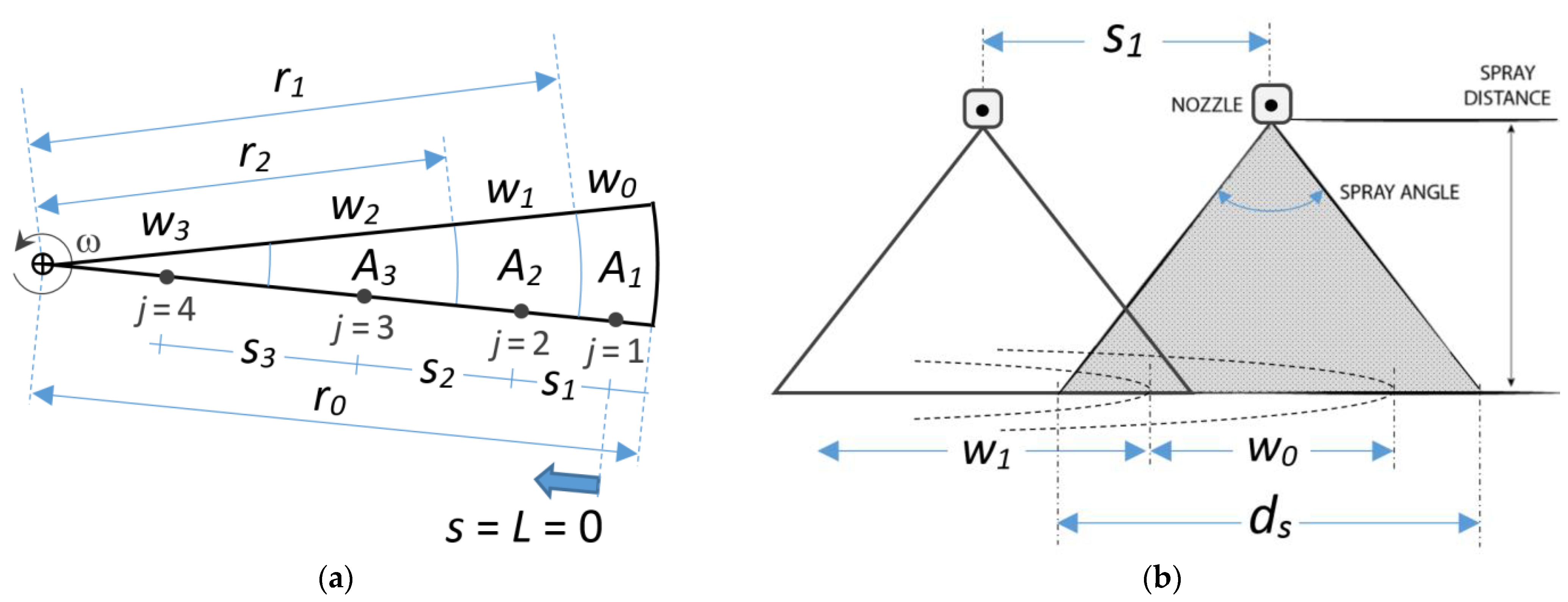
Along a given CPIS with radius, r0 (m), Baiamonte et al. [26] considered a lateral where N sprinklers, j = 1, 2, … N, with gradually decreased sprinkler spacing, s1, s2, … sN, are installed (Figure 1).
During the lateral rotation, with angular velocity ω, each sprinkler j fully irrigates an annulus area with gradually decreased width, w0, w1, … wN-1. The annulus area irrigated by each sprinkler j, A, was imposed equal for all the sprinklers, and it was expressed by the ratio between the design sprinkler flow rate, qn, and the desired water application rate, i:
Once a constant qn is fixed, Equation (1) states that for a uniform water application rate, i, a constant irrigated annulus area A, for each sprinkler installed with variable spacing (Figure 1), needs to be imposed. One parameter, A*, i.e., the annulus area, A, normalized with respect to the pivot irrigated area, , can be used to fully describe the CPIS geometric and the sprinkler flow rate characteristics:
For different values of r0 and qn parameters, Figure 2 shows A* as a function of the water application rate, i, indicating the high variability of A* (four orders of magnitude). The figure also reports the A* values corresponding to the applications, run #1 and run #2, that will be discussed later.
According to Equation (1), Baiamonte et al. [26] found the variable decreased sprinkler spacing sequence that needs to be imposed for a uniform water application rate, which, in this work, will be associated with the A* parameter (Equation (2)). For the first annulus, where the first outer sprinkler, j = 1, is installed (Figure 1), the width, w0, normalized with respect the CPIS radius, r0, can be expressed by using A* (Equation (2)), which Baiamonte et al. [26] did not consider:
Once w*0 is established, the normalized annulus width of the sprinklers after the first one (j > 1, Figure 1) was determined by imposing for each sprinkler a constant annulus area (A*), according to a recurrence relation that recursively defines a sequence of gradually decreasing annulus widths, associated with A*. The distance between the edge of each width and the center-pivot, rj (Figure 1), normalized with respect to r0, is denoted as r*j. Therefore, for the first annulus width, wide w0, the initial terms, r*0 = r0/r0 = 1 and w*0 (and A*, Equation (3)), are established, and the w*j sequence can be derived:
where r*j, w*j, r*j−1, and w*j−1 are the radius and annulus width corresponding to the sprinkler j and j−1, normalized with respect to lateral length, r0. Thus, each further term of the w*j sequence is defined as a function of the preceding terms and corresponds to a sequence of annuli characterized by a constant area, A, irrigated by each sprinkler, thus assuring a uniform water application rate.
Equation (4) also makes it possible to derive the sprinkler spacing sequence, which needs for the hydraulic design of the CPIS lateral. Indeed, considering that each sprinkler is in the middle of the annulus width (Figure 1) yields:
where s*j is the sprinkler spacing between the sprinkler j and j−1, normalized with respect to lateral length, r0. For N sprinklers, the corresponding normalized lateral length, L*, which is referred to the distal end of the lateral, starting from the outer sprinkler (Figure 1), equals to:
For different A* values, the cumulated w*j, ∑w*j and the cumulated s*j, ∑s*j are graphed in Figure 3a and in Figure 3b, respectively, as a function of the sprinkler number j, illustrating an expected monotonically increasing trend. Moreover, for a fixed A*, because of the radicand constrain in Equation (4), depending on the geometric and hydraulic CPIS characteristics, a lateral length fully covering the CPIS radius (∑w*j = 1) cannot always be achieved. Indeed, to fully cover the lateral length, different sprinkler characteristics, i.e., qn, should be considered. However, the latter issue is beyond the purpose of this paper, which aims to design CPIS laterals by only using different inside diameters.
Therefore, the cumulated sprinkler interspace displayed in Figure 3b can be applied to any pair or triplet of diameters of the CPIS lateral, and the two or more sectors in which the irrigated area is subdivided are only determined by the changes in lateral diameters.
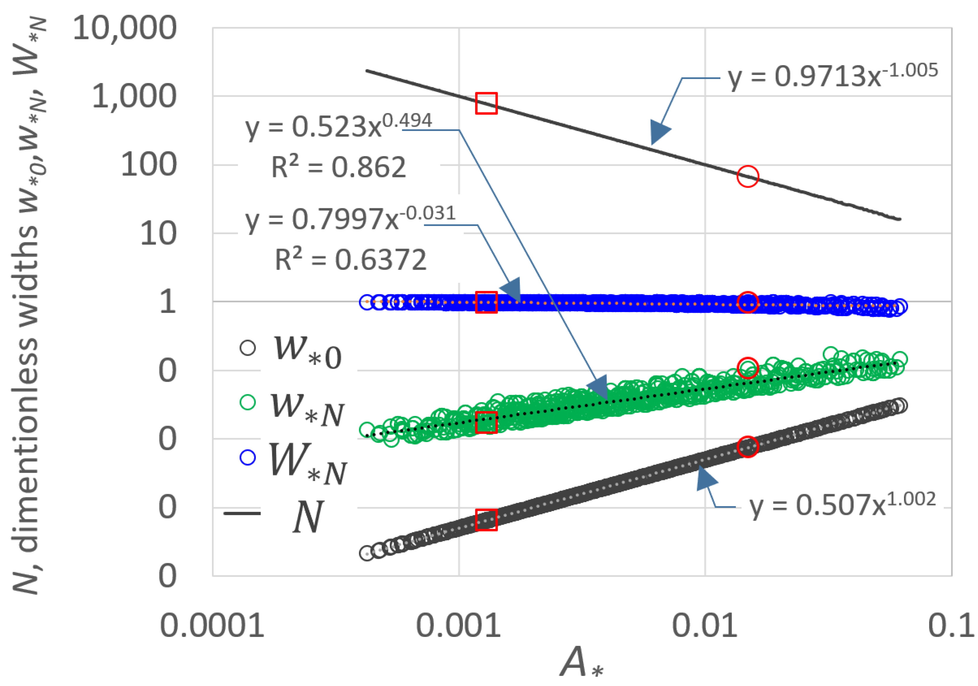
Of course, the number of sprinklers, N, which can be installed along the lateral is also affected by A*. For a high number of simulations performed for reasonable values of the triplet (i, r0, qn), N is graphed in Figure 4 versus A*, together with (see Figure 5): (i) the normalized width irrigated by the first sprinkler w*0 (Equation (3)), (ii) the normalized width irrigated by the last sprinkler w*N, and (iii) the normalized width irrigated by the total number of sprinklers, W*N:
Figure 4 shows that N versus A* (solid line) is fitted by a power law well, and, of course, so is w*0 (Equation (3)). Contrarily, W*N and w*N show a worse power-law fitting than N and w*0, which is due to the sequence annuli randomness in fully covering or not fully covering the entire pivot area, already discussed for Figure 3. However, it seems that the lower A* is, the more the total annuli width, W*N (blue circles), approaches the unity (fully coverage).
High values of A* values, greater than those displayed in Figure 4, could be not recommended because the corresponding high widths, w*0 and w*N, even for high spray distance (Figure 1b), might not be covered by one sprinkler, and thus, they should be preliminarily checked [26]. Figure 4 also illustrates the values corresponding to the applications run #1 and run #2 that will be performed later.
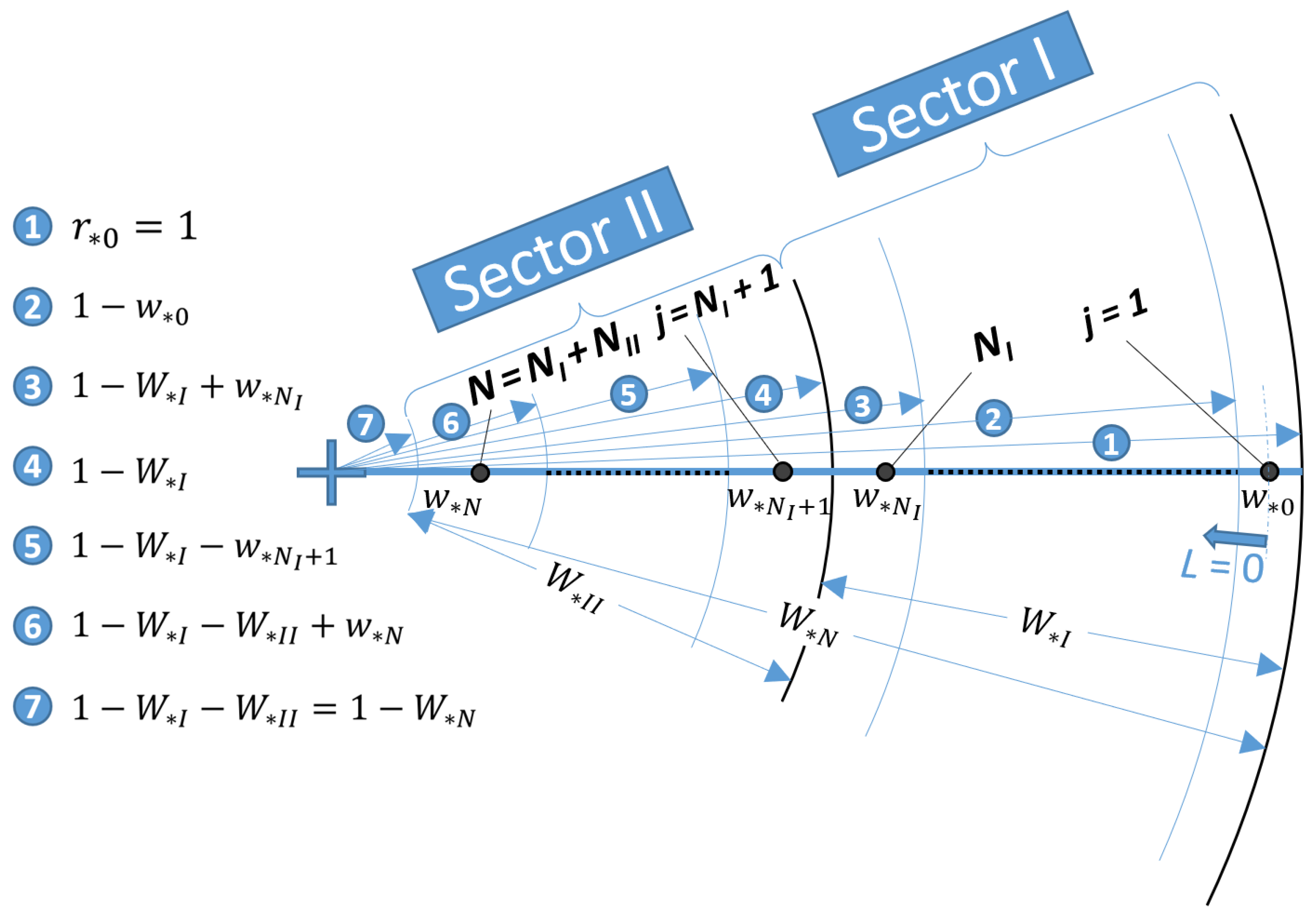
Telescoping laterals do not require to use the total number of sprinklers installed in the same pipe diameter, since the pipe diameter could be changed after a number of sprinkler NI < N, according to two or more than two sectors. For a clear legibility of the considered sketch, for the case of two sectors, i.e., dual-diameter lateral, Figure 5 illustrates the aforementioned parameters, w*0, w*N, W*N, where the subscript I refers to the sector I (outer lateral), whereas the subscript II refers to the sector II (inner lateral). The last sprinkler width, w*N, which belongs to a common w*j sequence of the two sectors (green circles in Figure 4), is associated with the total number of sprinklers, N = NI + NII.
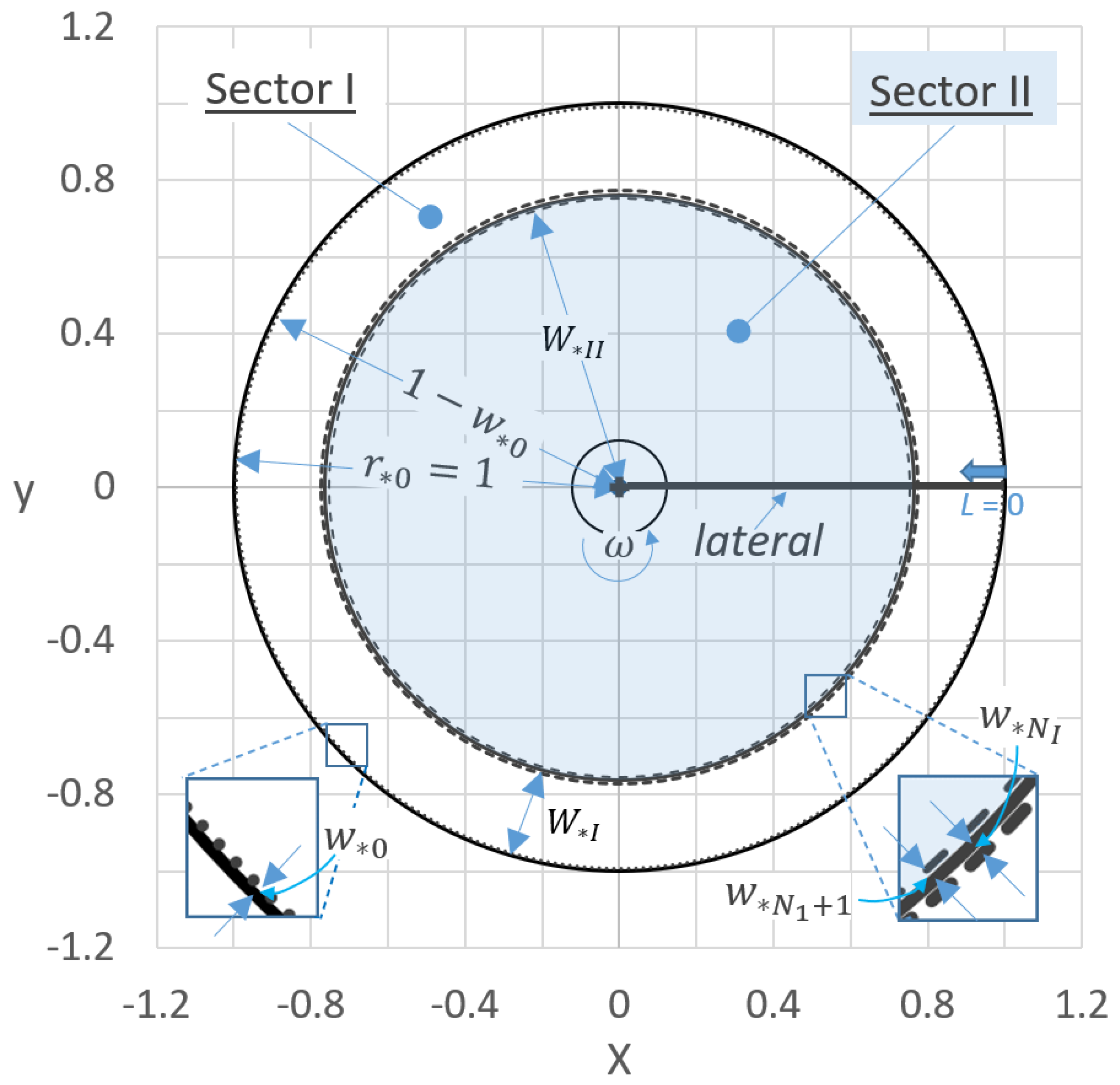
As an example, for run #1, where a number of sprinklers in sector I, NI = 28, was imposed (Table 1), Figure 6 shows the corresponding two sectors that could be geometrically designed with a dual-diameter lateral.
Hydraulic Design
Once the geometry of the center-pivot was designed, Baiamonte et al. [26] also provided an easy to apply hydraulic design procedure, starting from a simplified approach that Baiamonte [4] developed for drip laterals, according to the energy balance. Baiamonte et al. [26] described the pressure head distribution (PHD) line of the N sprinklers, under the assumption to neglect the variation of sprinkler flow rate, qn, along the lateral [29,30] and local losses, as generally assumed for the pivot laterals [31], which contrarily have to be considered in the drip laterals design.
The CPIS design procedure suggested by Baiamonte et al. [26] for one-diameter lateral could be extended for three or more sectors, but for a simplified description of the procedure, only two sectors will be considered here. Under constant qn, for sector I and for sector II, i.e., for the outer lateral and for the inner laterals (Figure 5 and Figure 6), the PHD line can be expressed as:
respectively, where h*j is the pressure head at the sprinkler j; h*min is the minimum pressure head to be imposed at the first sprinkler j = 1, both normalized with respect to r0, hj/r0 and hmin/r0, respectively; and KI and KII denote the parameters of sector I and of sector II, accounting for the friction losses (friction head loss gradient) and according to the well-accepted Hazen–Williams’s resistance equation [5,32], also recently considered for CPIS [33]:
where DI (m) and DII (m) are the inside diameters of the outer lateral and of the inner laterals (sector I and II), respectively, and C is a pipe smoothness factor, which is a function of the pipe material’s characteristics [32,34].
For drip laterals, Baiamonte [4] showed that based on the energy balance equation, where the hypothesis to neglect the variation of sprinkler flow rate was assumed, the design problem of drip laterals can be solved by imposing a fixed pressure head tolerance, δ, which depends on the desired emission uniformity coefficient of Keller and Karmeli [35]. Baiamonte [4] also derived analytical solutions that facilitate the micro-irrigation design for one-lateral units [4,36] as well as for rectangular micro-irrigation units [37].
For CPIS, a similar approach as that described for drip laterals, for a fixed minimum normalized pressure head, h*min, the maximum pressure head at j = NI, normalized with respect to r0 and denoted as h*n (Figure 7a), can be imposed to delimit the PHD line in the range h*min ≤ h*j ≤ h*n:
Denoting δI the pressure head tolerance assumed for sector I, the normalized average pressure h*n,I (Figure 7a) can be used to express h*min and h*n, respectively:
Using Equations (13) and (14), h*n can be expressed as a function of h*min:
Substituting Equation (15) into Equation (10) provides:
For sector II, denoting h*max and δΙΙ, the maximum normalized pressure and the pressure head tolerance for the inner lateral, a similar relationship to Equation (16) can be derived, if considering that the maximum normalized pressure of sector I, h*n, corresponds the minimum normalized pressure head of sector II (Figure 7a), providing:
where h*n,II is the average normalized pressure head for the inner lateral (Figure 7a). Using Equations (17) and (18), h*max can be expressed as a function of h*n:
The normalized maximum pressure head (Equation (19)) can also be expressed as a function of h*min by using Equation (15):
For run #1, where δI = 0.02 was imposed, h*min, h*nI, h*n, h*nII, and h*max values are also reported in Figure 7a, together with their average h*av = 0.5 (h*max + h*min), which will be considered later to evaluate the corresponding coefficient of variation of the pressure heads around hav, CVav.
To delimit the PHD variation in sector II (h*n ≤ h*j ≤ h*max, Figure 7a), and thus the sprinkler flow rate variations, as for sector I, h*max can be imposed at the distal end of the lateral (j = N = NI + NII) in the corresponding energy balance equation (Equation (9)), which by using Equation (12) provides:
Equation (21) makes it possible to determine the KII relationship:
Finally, substituting Equations (15) and (20) into Equation (22), the KII parameter as a function of h*min can be obtained:
Since h*max also represents the normalized pressure head that the pump system has to provide at the inlet, h*max ≡ h*min, by using Equation (20), it is also useful to express KI and KII as a function of h*in:
In conclusion, for fixed δI and δII, the K values for the inner and the outer lateral, KI and KII, can be expressed according to any fixed h*min value (Equations (16) and (23)) or to any fixed h*in value (Equations (24) and (25)), once A* (Equation (2)) and any pair of pressure head tolerances (δI, δII), are assumed. Of course, the CPIS pressure head tolerance, δ, is equal to δI + δII. Importantly, for any input data, in the K relationships, the mathematical formulation of the principle of the conservation of energy for the lateral of a Center-Pivot is satisfied, so that the pressure head variation is balanced by the sum of friction losses in between the sprinklers.
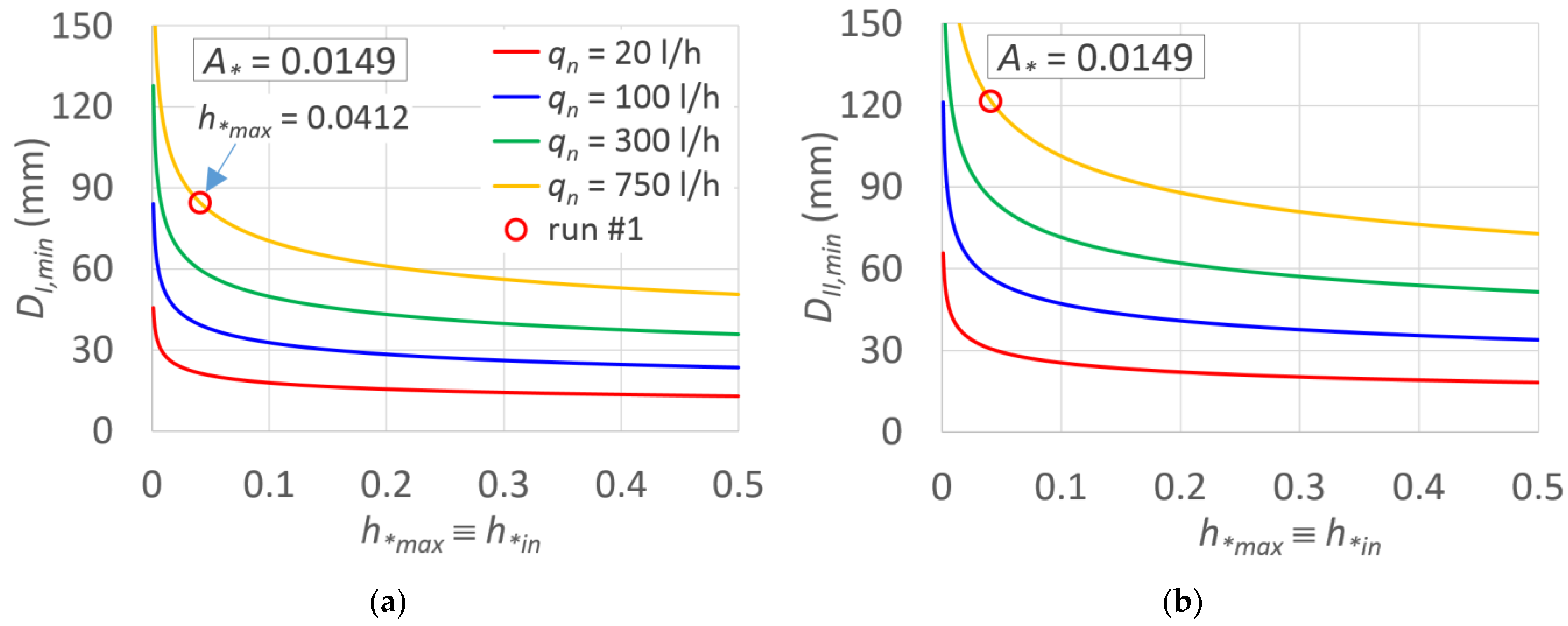
Knowledge of KI and KII values allows for designing the inner and the outer lateral diameters, by inverting Equations (10) and (11):
The hypothesis to neglect the variation of sprinkler flow rate, qn, when deriving K relationships, agrees with the assumption to impose a pressure head tolerance δI and δII. In fact, along a lateral where sprinklers are installed, it is under limited pressure head variations established by the pressure head tolerances that the ratio between the sprinkler flow rate variation (qmax–qmin), and its average, qn, is low (for x = 0.5, it equals to 5%, when δ = 10 %), providing a good approximation of this assumption [38,39].
3. Applications
For run #1, where A* = 0.0149 and r0 = 400 m (Table 1) were assumed; for fixed pressure heads tolerances δI = 0.02 and δII = 0.08, so that the CPIS pressure head tolerance δ = δI + δII = 10%, as it is usual; for a fixed hmin = 13.5 m (h*min = 0.0338); and for NI = 28, Table 2 reports all the design variables previously introduced, in particular the cumulated sprinkler spacing ∑s*j,I and ∑s*j,II and the corresponding terms ∑s*j,I (j − 1)1.852 and ∑s*j,II (j − 1)1.852, which are required into the K relationships (Equations (24) and (25)).
The latter parameters make it possible to calculate the inside diameters of the telescoping lateral, DI and DII (Table 2), by Equations (26) and (27), which resulted in 82.79 mm and 120.58 mm, respectively. Thus, as it is commonly accepted in practice, this dual-diameter case involves using a larger diameter pipe at the beginning of the lateral and then a lower diameter, as the flow rate decreases starting from the pivot axes.
Table 2 also reports the same parameters for the one-diameter lateral (K and D), where only Equation (16) was applied to the total number of sprinklers (N = 67) in order to make a comparison between one-diameter and dual-diameter CPISs.
Towards this aim, for a dual-diameter lateral, the mean weight diameter, Dm, which could be considered as an index of the investment costs, is also reported in Table 2. Dm was calculated as:
where L*,I = LI/L and L*II = LII/L. Of course, for a CPIS irrigated area fully covered by the sprinklers, the denominator of Equation (28) is equal to the unity.
To compare one-diameter and dual-diameter CPISs, the corresponding relative difference between one-diameter (D) and dual diameter (Dm) laterals, RED, was calculated as:
For run #1, Table 2 shows that Dm is 4.5% less than the diameter, D, corresponding to a one-diameter lateral design. Of course, Dm could be used to roughly detect the most convenient choice of the diameter pair to be considered in the design by an economic point of view, since the lower Dm is, the lower the telescoping pipe cost will be [40,41]. However, a deeper economic analysis should be recommended, since the cost pipe does not necessary vary linearly with the diameter and for the best choice of the lateral diameters, the cost of reducing coupling or adapter should also be considered.
3.1. Numerical Validation
Testing the derived KI and KII relationships requires the corresponding PHD lines to be determined, by considering that, for the outer lateral, the PHD line can be expressed by (Equation (8)), whereas the inner lateral requires the application of Equation (9). For run #1, Figure 7 shows the corresponding PHD lines for both one-diameter and dual-diameter laterals in dimensionless (Figure 7a) and dimensional terms (Figure 7b), together with the PHD derived by the commonly used step-by-step (SBS) procedure (dots), which is rigorous since it considers the continuity and the motion equations repetitively applied to the consecutive sprinkler outlets and the actual sprinkler flow rate–pressure head relationship. The comparison showed in Figure 7 indicates the reliability of the described procedure.
Indeed, for the fixed h*min = 0. 0338, the PHD line achieves the normalized pressure head in the changing section (h*n = 0.0351) calculated by Equation (16), and then the maximum normalized pressure, h*max = 0.0412, is achieved at the distal sprinkler of the lateral.
The comparison was performed for an exponent x = 0.5 of the sprinkler flow rate–pressure head relationship, commonly assumed for sprinklers, thus for a coefficient ke = qn/√hn = 200.08 l h−1 m−0.5, which was set equal for both dual- and one-diameter laterals (Table 2). Of course, for x = 0, the solutions provided by the suggested procedure matches that provided by SBS, and it has no sense to be compared. Figure 7 also reports the PHD derived by the suggested procedure and by the SBS method, in the case of a one-lateral diameter.
It is interesting to consider that the pivot radius is a scale factor of the aforementioned relationships; thus, the results presented here could be referred to any pressure head–pivot radius pair, providing the same normalized values. Indeed, once the telescoping pipe is designed and the normalized PHD line determined, the PHD line in dimensional terms can be simply derived by multiplying the normalized pressure heads for the selected r0 value.
3.2. Varying the Pressure Head Tolerances
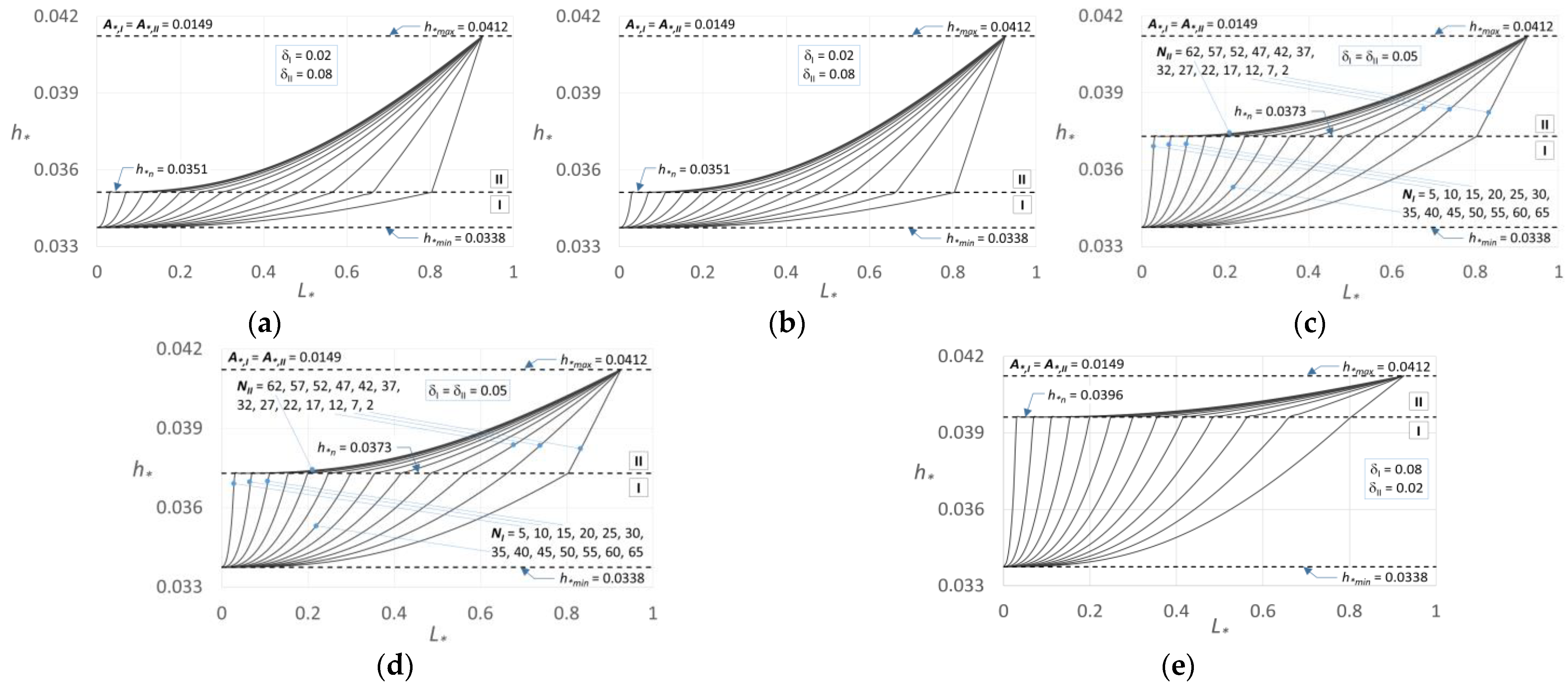
In order to investigate the influence of pressure head tolerances δI (and δII) and of the number of sprinklers installed in the first (NI) and in the second sectors (NII), for run #1, further applications have been performed. By varying the pressure tolerances, δI = 0.02, 0.04, 0.05, 0.06, and 0.08, and NI (and NII), Figure 8a–e show the corresponding PHDs, all laying in the admitted range (h*min ≤ h*j ≤ h*max), indicating that different pairs of the inside diameters could be selected, providing suitable behaviors in terms of sprinkler pressure head distribution.
For δI = 0.05, i.e., h*n ≡ h*av, which could be a good choice for constant interspace sprinklers, Figure 8c shows that for an equally distributed number of sprinklers (e.g., NI = 35), the PHD is not uniform. This because of the high variability in the sprinklers’ interspace, s (Figure 3), which needs to be imposed in CPISs for a uniform water application rate.
Before comparing the output design diameters for dual- and one-lateral CPISs, an error analysis on pressure heads, aimed at detecting the suitability of the suggested procedure, has been performed. In particular, relative errors, RE, corresponding to the normalized pressure according to the suggested procedure and according to SBS were calculated for dual-diameter laterals at the changing diameter section, RE(h*n)dual, and at the inlet, RE(h*max)dual, whereas for one-diameter laterals, REs were calculated at the maximum pressure section, RE(h*max)one:
where h*PS is the normalized pressure head according to the present solution, and h*SBS is the corresponding value according to the SBS procedure, where x = 0.5 was imposed.
For run #1, by varying NI and δI, Table 3 reports RE(h*n)dual, RE(h*max)dual, and RE(h*max)one, which, of course, does not depend on NI and δI. The results show that for dual-diameter, REs are almost slight (generally lower than for one-diameter), and for any NI, REs decrease at decreasing δI. Bold values refer to the maximum RE, which was less than 2.28%, thus demonstrating a good approximation of the exact SBS procedure.
Once the error analysis has been performed, for run #1 (Figure 8), the design diameters have been compared. For run #1, Table 4 reports DI and DII values together with the mean weight diameters Dm (Equation (28)), which generally resulted in being lower than those corresponding to one lateral diameter (D = 116.45 mm).
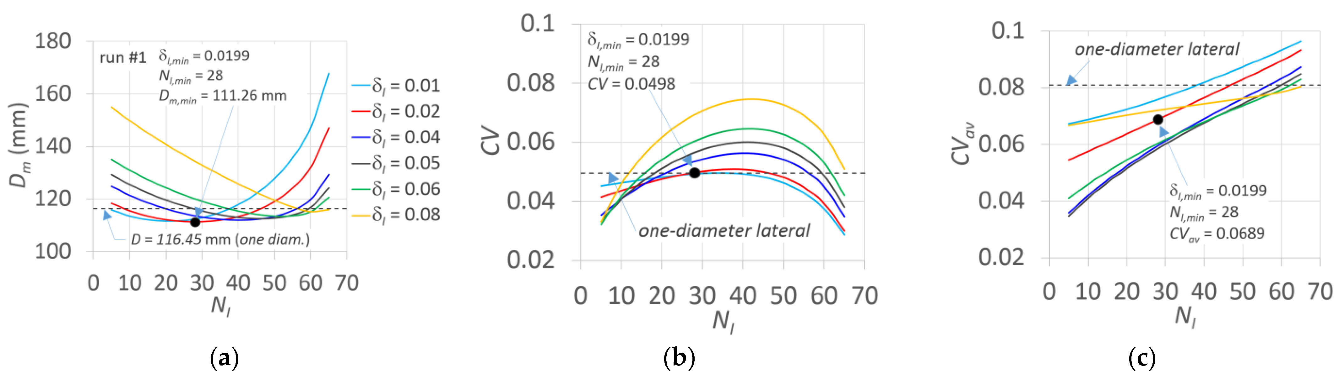
Dm values that resulted in being higher than D (116.45 mm, Table 2) are in bold, whereas the lowest Dm value (Dm,min = 111.26 mm, bold and underline) is obtained for NI,min = 28 and δI,min = 0.02, indicating that the application illustrated in Figure 7 could be the most convenient choice from an investment cost point of view. For a few cases, for high NI values, uncommon DI < DII conditions occur, and the corresponding DI values are highlighted by an asterisk. These cases can be observed in the corresponding PHD slopes (Figure 8). For example, compare the case δI = 0.06 and NI = 65 with the corresponding PHD line reported in Figure 8d.
The minimum mean weight diameter, Dm,min, can also be observed in Figure 9a, where Dm is plotted as a function of NI, for different δI values. Figure 9a shows that for some of the considered NI and δI values, Dm is higher than D (116.45 mm, dashed line), and that the higher Dm values are associated with low and high NI values. Thus, NI and δI need to be accurately selected to obtain a desirable design. The latter could also be analyzed in terms of the coefficient of variation of the pressure heads, as it is described in the following.
Figure 9b plots the coefficient of variation of pressure heads with respect to the mean of the PHD values (h*j), indicating that, contrarily to Figure 9a, the lowest CV values, which are lower than the CV = 0.0498 obtained for one lateral diameter (dashed line), occur for low and high NI values. However, it needs considering that for dual-diameter laterals, CV values that are higher than for a one-diameter lateral is an expected issue, since it is associated with the abrupt modification of the PHD due to the changing diameter (Figure 7 and Figure 8). A more suitable comparison in terms of the coefficient of variation could be performed with respect to the average pressure head, h*av, calculated according to the minimum and maximum values, h*av = 0.5 (h*max + h*min):
where CVav is the variation coefficient calculated with respect to hav. This because hav refers to a linear PHD providing a uniform distribution of sprinkler flow rate and can be selected as a reference to evidence the benefit of the dual-diameter laterals.
Towards this aim, Figure 9c graphs CVav as a function of NI for the same δI previously considered, evidencing the benefit of a dual-lateral diameter in terms of PHD around the average h*av value. Indeed, with exception of few cases, the CVav calculated for dual-diameter lay below that for one-diameter lateral (dashed line).
Of course, these results have to be referred to the corresponding A* value selected (0.0149), and further applications are needed to investigate the suggested procedure for a wider range of the input parameters.
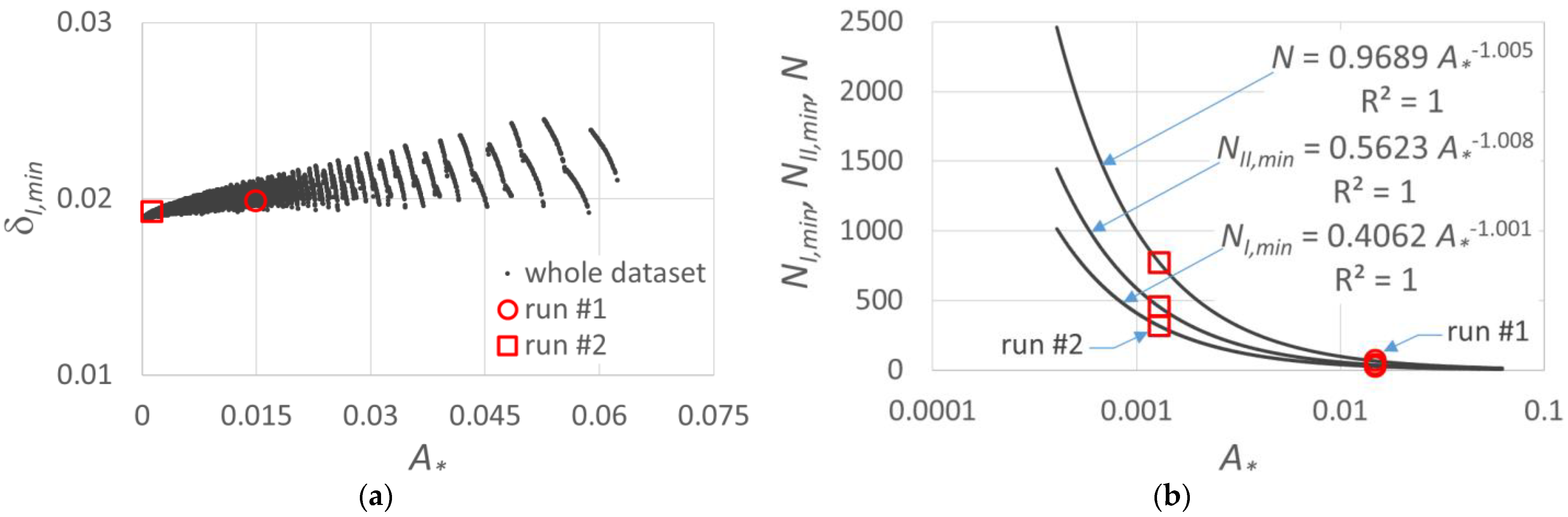
Therefore, a generalization of the results illustrated in Figure 9 was performed for a very high number of simulations (15,000) characterized by different values of the A* parameter, which describes the geometry of the CPIS. The triplet of values (qn, r0, i) was selected according to their common ranges also considered in Baiamonte et al. [26] in order to arrange a whole reliable dataset. For each simulation, the Dm,min value was calculated according to an objective function by minimizing Dm and by varying NI and δI:
Figure 10a illustrates that at increasing A*, a slight increase in δmin,I occurs, and that δI is close to 0.02 (Figure 8a), which is reasonable, if considering that the outer laterals are characterized by larger areas to irrigate than the inner laterals. Thus, δI = 0.02 could be a good approximation of the recommended value to obtain the lowest Dm. The number of sprinklers to be installed in the first sector, NI,min (and in the second sector, NII,min), are power-laws, as illustrated in Figure 10b; thus, they could be used for an easy CPIS design.
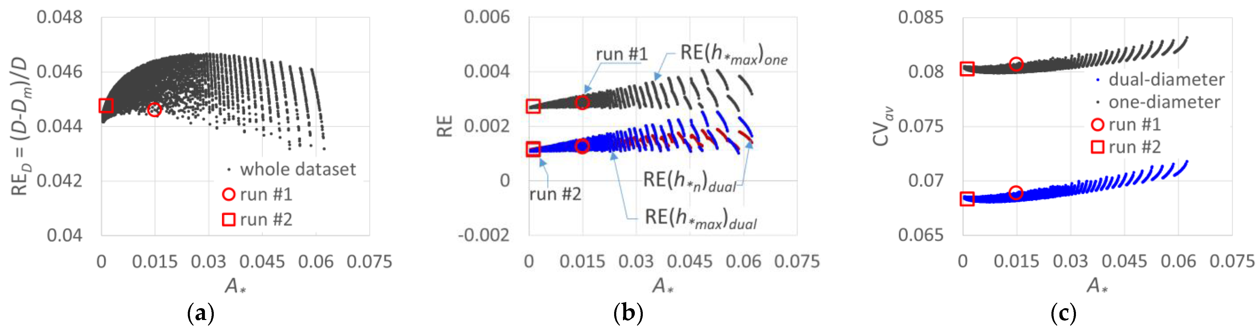
For the whole dataset considered in Figure 10, Figure 11a shows that by varying A* (different CPIS geometries), RED varies in a narrow range (0.043–0.047). Thus, Dm results in being almost 4.5 % lower than D, thereby confirming the result obtained for run #1 (Table 2).
Figure 11b plots the relative errors in pressure heads, RE(h*n)dual and RE(h*max)dual (Equation (30)) versus A*, which makes it possible to conclude that the previous RE range (<2.28%, Table 3) is much lower and almost negligible (<0.3 %), if referred to the considered Dm,min (Equation (32)). For the maximum pressure head in the case of one-diameter lateral, RE(h*max)one, a bit higher RE values were obtained (Figure 11b).
Although low RED were observed (Figure 11a), a more significant effect of the dual-diameter can be observed in terms of CVav (Equation (31)). For both one and dual-diameters and for the whole dataset, in Figure 11c, CVav is plotted versus A*. The figure shows that for one-diameter laterals, CVav is higher (≅0.083) than for dual-diameters laterals (≅0.068), indicating more suitable PHDs for the latter. Figure 11 also indicates the dots corresponding to the applications run #1 and run #2 that will be performed in Section 3.4.
3.3. Varying the Inlet Pressure Head
The normalized inlet pressure, h*in, which was set equal for the whole dataset (h*in = 0.0412, Table 2), also plays an important role in the suggested CPIS design procedure. Using Equations (24) and (25), it can be easily observed that h*in is a scale factor of the K relationships. For run #1 (A* = 0.0149), Figure 12a,b plot the diameter of sector I, DI, and sector II, DII, by varying h*in with qn as a parameter. As expected, lower DI and DII values could be selected for normalized inlet pressures higher than that considered for run #1 (dot circles), and these values further decrease with decreasing qn.
3.4. Application for Run #2
Finally, for a different set of the input parameters reported in Table 1 (run #2), another application aimed at summarizing the suggested procedure was performed. Due to the higher lateral length (r0 = 700 m) than run #1 (r0 = 400 m), an inlet pressure, hin = 25 m, higher than 16.5 m (fixed for run #1) was set. For the selected qn = 300 l/h and i = 0.15 mm/h, A* equals 0.0013 (Equation (2), Table 1). First, for A* = 0.0013, the annulus width sequence irrigated by each sprinkler (Equations (3) and (4)) was derived. Second, the number of sprinklers in the first sector NI has to be determined by the equation displayed in Figure 10b, and approximating to the integer, 316 sprinklers were obtained.
According to the results shown in Figure 10a, which suggests that the pressure head tolerance of the outer lateral is close to 0.02, when the minimum weight diameter is imposed, δI = 0.02 and δII = 0.08 were selected, in order to set the pressure head tolerance of the dual-diameter lateral δ = δI + δII = 0.1. Once the parameter ∑s*j,I (j − 1)1.852 and ∑s*j,II (j − 1)1.852, which are required in K relationships are calculated (Table 2), for C = 135, the corresponding sectors’ diameters were determined by Equations (26) and (27), providing DI = 152.1 mm and DII = 224.8 mm. Of course, these diameter values do not match the available commercial ones; however, commercial pipe diameters immediately larger than the design ones could be selected, which will provide δ < 0.1. Since the latter is beyond the purpose of this study, in the following, the design diameter values (DI = 152.1 mm and DII = 224.8 mm) are considered to compare the suggested procedure and the exact one provided by the numerical step-by-step (SBS) method.
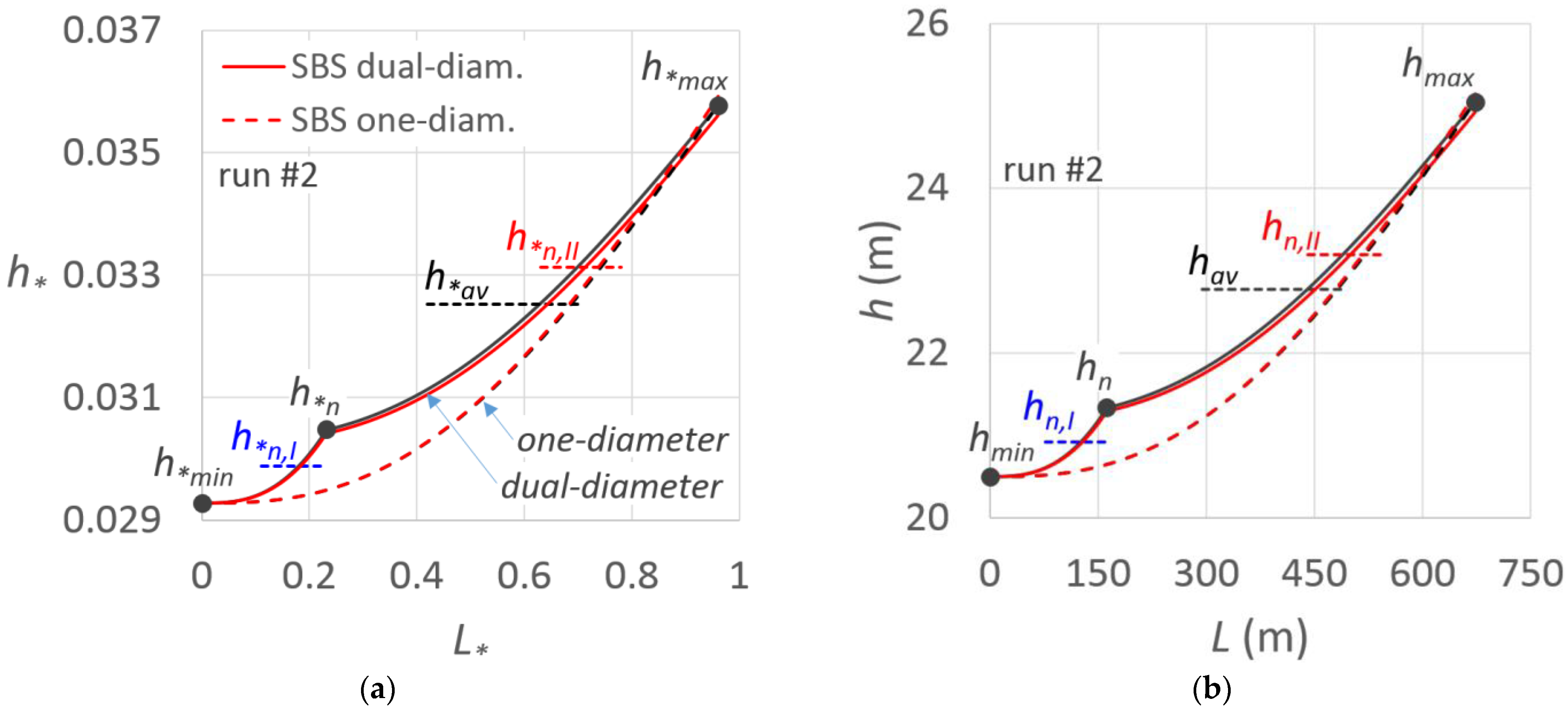
For run #2, Figure 13 plots the PHD lines obtained for dual-diameter laterals and for the one-diameter lateral for the suggested procedure and by the SBS method, confirming that, for fixed pressure-head tolerances δI and δII, neglecting the flow variation in the approximate design procedure determines very moderate errors in PHD lines and makes it possible to achieve the established pressure head extremes (hmin and hmax, Table 2). The suggested procedure also provides convenient solutions from an energy-saving point of view. Indeed, it was observed that confining the sprinkler pressure heads into an admitted range, and thus the sprinkler flow rates, favors high emission uniformity and, as for drip laterals, allows one to also save energy [6].
4. Conclusions
This paper extends a simple procedure to design Center-Pivot irrigation systems for gradually decreased sprinkler spacing along the pivot lateral, which was suggested for one-diameter lateral, to two lateral diameters. The results showed that, according to the design criteria and for the assigned input parameters, many solutions can be selected by varying the sprinkler characteristics and/or the pipe diameters, the pressure head tolerances, and the number of sprinklers of the dual-diameter laterals. The minimum value of the mean weight diameter, which could be considered a coarse indicator of the lowest investment costs, results in a bit lower value (4.5%) than that corresponding to a one-diameter lateral, and it is obtained when the pressure head tolerance of the outer lateral, δI, equals 2%, which is reasonable if considering that the outer laterals are characterized by larger areas to irrigate than the inner lateral. For δI = 0.02, an error analysis showed that the relative error, RE, between the sprinkler pressure heads, evaluated according to the suggested procedure and those evaluated by the numerical and exact step-by-step procedure are lower than 0.4 %, thus validating the suggested approach. For some practical cases, applications of the proposed procedure were performed and discussed. Although the procedure was presented, applied, and tested for dual-diameter laterals, it could be easily extended to three or more pipe diameters.
Funding
This research received no external funding.
Institutional Review Board Statement
Not applicable.
Data Availability Statement
The data presented in this study are available on request from the corresponding author.
Acknowledgments
The author wishes to thank the anonymous reviewers for their helpful comments and their careful reading of the manuscript during the revision stage.
Conflicts of Interest
The author declares no conflict of interest.
List of Symbols
| A [L2] | = area irrigated by each sprinkler |
| A0 [L2] | = pivot irrigated area |
| A* | = area irrigated by each sprinkler normalized with respect to the pivot irrigated area |
| C | = pipe smoothness factor |
| CV | = variation coefficient of pressure heads |
| CVav | = variation coefficient calculated with respect to hav. |
| D [L] | = inside diameter of the one-diameter lateral |
| Dm [L] | = mean weighted diameter |
| Dm,min [L] | = minimum value of the mean weighted diameter |
| DI [L] | = inside diameter of the lateral of the outer lateral |
| DII [L] | = inside diameter of the lateral of the inner lateral |
| hj [L] | = pressure head at the j-th sprinkler |
| hav [L] | = average pressure head |
| hmin [L] | = minimum admitted pressure head |
| hmax [L] | = maximum admitted pressure head |
| hn [L] | = nominal pressure head |
| h*av | = normalized average pressure head |
| h*in | = inlet pressure head normalized with respect to r0 (equals to h*max) |
| h*j | = pressure head at the j-th sprinkler normalized with respect to r0 |
| h*max | = maximum allowable pressure head normalized with respect to r0 |
| h*min | = minimum allowable pressure head normalized with respect to r0 |
| h*n | = average pressure head normalized with respect to r0 (it matches the normalized pressure head in the changing section, for dual-diameter laterals) |
| h*n,I | = average pressure head normalized with respect to r0 of the outer lateral (sector I) |
| h*n,II | = average pressure head normalized with respect to r0 of the inner lateral (sector II) |
| h*PS | = normalized pressure head according to the present solution |
| h*SBS | = normalized pressure head according to the SBS procedure |
| I [L T−1] | = water application rate |
| ke [L3 T−1 L−0.5] | = coefficient of the sprinkler flow rate–pressure head relationship |
| KI | = friction head loss gradient of the outer lateral |
| KII | = friction head loss gradient of the inner lateral |
| L [L] | = length of the Center-pivot lateral |
| L* | = length of the Center-pivot lateral normalized with respect to r0 |
| N | = number of sprinklers |
| NI | = number of sprinklers of the outer lateral of the telescoping pipe |
| NI,min | = number of sprinklers of the outer lateral corresponding to Dm,min |
| NII | = number of sprinklers of the inner lateral of the telescoping pipe |
| NII,min | = number of sprinklers of the inner lateral corresponding to Dm,min |
| qn [L3 s−1] | = design flow rate of the sprinkler |
| r0 [L] | = radius of the Center-pivot |
| rj [L] | = radius corresponding to the sprinkler j |
| r*j | = radius corresponding to the sprinkler j normalized with respect to r0 |
| s1 [L] | = sprinkler spacing between the sprinkler j and the sprinkler j − 1 |
| s*j | = sprinkler spacing between the sprinkler j and the sprinkler j − 1 normalized with respect to r0 |
| wj [L] | = annulus width of the sprinkler j |
| w*j | = annulus width of the sprinkler j normalized with respect to r0 |
| w0 [L] | = annulus width of the first sprinkler (j = 1) |
| wN [L] | = annulus width of the last sprinkler N |
| w*0 | = annulus width of the first sprinkler (j = 1) normalized with respect to r0 |
| W*N | = normalized width irrigated by the total number of sprinklers |
| x | = exponent of the sprinkler flow rate–pressure head relationship |
| δ | = pressure head tolerance |
| δI | = pressure head tolerance of the outer lateral (sector I) |
| δI,min | = pressure head tolerance corresponding to Dm,min |
| δII | = pressure head tolerance of the inner lateral (sector II) |
| ω rad [T−1] | = angular velocity |
References
- Levidow, L.; Zaccaria, D.; Maia, R.; Vivas, E.; Todorovic, M.; Scardigno, A. Improving water-efficient irrigation: Prospects and difficulties of innovative practices. Agric. Water Manag. 2014, 146, 84–94. [Google Scholar] [CrossRef] [Green Version]
- Noreldin, T.; Ouda, S.; Mounzer, O.; Abdelhamid, M.T. CropSyst model for wheat under deficit irrigation using sprinkler and drip irrigation in sandy soil. J. Water Land Dev. 2015, 26, 57–64. [Google Scholar] [CrossRef] [Green Version]
- Al-Samarmad, O.T. Optimum Dimension of a Trickle Irrigation Subunit by Using Local Prices. Master’s Thesis, Department of Irrigation and Drainage Engineering, College of Engineering, University of Baghdad, Baghdad, Iraq, 2002. [Google Scholar]
- Baiamonte, G. Advances in designing drip irrigation laterals. Agric. Water Manag. 2018, 199, 157–174. [Google Scholar] [CrossRef]
- Sadeghi, S.H.; Peters, R.; Lamm, F. Design of Zero Slope Microirrigation Laterals: Effect of the Friction Factor Variation. J. Irrig. Drain. Eng. 2015, 141, 04015012. [Google Scholar] [CrossRef]
- Baiamonte, G. Minor Losses and Best Manifold Position in the Optimal Design of Paired Sloped Drip Laterals. Irrig. Drain. 2018, 67, 684–701. [Google Scholar] [CrossRef]
- FAO, Food and Agriculture Organization of the United Nations Food & Agriculture Organization. Technology & Engineering Side Event: Engaging agriculture, forestry and fisheries in the 2030 Agenda: A guide for policymakers. In Proceedings of the 159th Session of the Council, Rome, Italy, 4–8 June 2018; FAO Headquarters (Sheikh Zayed Centre): Rome, Italy, 2018; 27, p. 64. [Google Scholar]
- Bradley, A.K.; Kincaid, D.C. Cooperative Extension System, Agricultural Experiment Station; BUL 797; College of Agriculture, University of Idaho: Moscow, ID, USA, 1997. [Google Scholar]
- Islam, Z.; Mangrio, A.G.; Ahmad, M.M.; Akber, G.; Muhammad, S.; Umair, M. Application and distribution of irrigation water under various sizes of center pivot sprinkler systems. Pak. J. Agric. Res. 2017, 30, 1. [Google Scholar]
- Schneider, A.D. Efficiency and uniformity of the LEPA and spray sprinkler methods: A review. Trans. ASAE 2000, 43, 937–944. [Google Scholar] [CrossRef]
- Gan, L.; Rad, S.; Chen, X.; Fang, R.; Yan, L.; Su, S. Clock Hand Lateral, A New Layout for Semi-Permanent Sprinkler Irrigation System. Water 2018, 10, 767. [Google Scholar] [CrossRef] [Green Version]
- Kincaid, D.C. Application rates from center pivot irrigation with current sprinkler types. Am. Soc. Agric. Eng. 2005, 21, 605–610. [Google Scholar] [CrossRef]
- Reddy, J.M.; Apolayo, H. Friction Correction Factor for Center-Pivot Irrigation Systems. J. Irrig. Drain. Eng. 1988, 114, 183–185. [Google Scholar] [CrossRef]
- Scaloppi, E.J.; Allen, R.G. Hydraulics of Center-Pivot Laterals. J. Irrig. Drain. Eng. 1993, 119, 554–567. [Google Scholar] [CrossRef]
- Faci, J.M.; Salvador, R.; Playán, E.; Sourell, H. Comparison of Fixed and Rotating Spray Plate Sprinklers. J. Irrig. Drain. Eng. 2001, 127, 224–233. [Google Scholar] [CrossRef] [Green Version]
- Rogers, D.H.; Aguilar, J.; Kisekka, I.; Lamm, F.R. Center pivot irrigation system losses and efficiency. In Proceedings of the 29th Annual Central Plains Irrigation Conference, Burlington, CO, USA, 21–22 February 2017. [Google Scholar]
- Bagarello, V.; Baiamonte, G.; Caia, C. Variability of near-surface saturated hydraulic conductivity for the clay soils of a small Sicilian basin. Geoderma 2019, 340, 133–145. [Google Scholar] [CrossRef]
- Evans, R.G. Irrigation Technologies. Sidney, Montana, June 2006. Available online: https://www.ars.usda.gov/ARSUserFiles/30320500/IrrigationInfo/general%20irrigation%20systems-mondak.pdf (accessed on 7 January 2019).
- Valín, M.I.; Cameira, M.R.; Teodoro, P.R.; Pereira, L.S. DEPIVOT: A model for Center-Pivot design and evaluation. Comput. Electron. Agric. 2012, 87, 159–170. [Google Scholar] [CrossRef]
- de Almeida, A.N.; Coelho, R.D.; Costa, J.O.; Farías, A.J. Methodology for dimensioning of a center pivot irrigation system operating with dripper type emitter. Eng. Agríc. 2017, 37, 4. [Google Scholar] [CrossRef] [Green Version]
- Baiamonte, G.; Baiamonte, G. Using Rotating Sprinkler guns during Center-Pivot Irrigation System. Irrig. Drain. 2019, 68, 893–908. [Google Scholar] [CrossRef]
- Majumdar, D.K. Irrigation Water Management: Principles and Practice; Asoke, K., Ghosh, P.H.I., Eds.; Learning Private Limited, M-97, Connaught Circus, New Delhi-110001; Meenakshi Art Printers: Delhi, India, 2000. [Google Scholar]
- Howell, T.A. Sprinkler package water loss comparisons. In Proceedings of the 2003 Central Plains Irrigation Conference, Sterling, CO, USA, 4–5 February 2003; Volume 760, pp. 54–69. Available online: https://www.ksre.k-state.edu/irrigate/oow/p04/Howell.pdf (accessed on 8 January 2022).
- Allen, R.G.; Keller, J.; Martin, D. Center Pivot System Design; The Irrigation Association: Falls Church, VA, USA, 2000; 300p. [Google Scholar]
- Chu, S.T. Center Pivot Irrigation Design. Agric. Exp. Stn. Tech. Bull. 1980, 61, 56. Available online: http://openprairie.sdstate.edu/agexperimentsta_tb/61 (accessed on 28 March 2017).
- Baiamonte, G.; Iovino, M.; Provenzano, G.; Elfahl, M. Hydraulic design of the Center-Pivot irrigation system for gradually decreased sprinkler spacing. J. Irrig. Drain. Eng. 2021, 147, 04021027. [Google Scholar] [CrossRef]
- Sadeghi, S.H.; Mousavi, S.F.; Sadeghi, S.H.R.; Abdolali, M. Factor H for the Calculation of Head Loss and Sizing of Dual-diameter Laterals. J. Agr. Sci. Tech. 2012, 14, 1555–1565. [Google Scholar]
- New, L.; Fipps, G. Center Pivot Irrigation. 2000. Available online: http://hdl.handle.net/1969.1/86877 (accessed on 10 January 2022).
- Christiansen, J.E. Irrigation by sprinkling. Calif. Agric. Exp. Stn. Tech. Bull. 1942, 670, 124. [Google Scholar]
- Zayani, K.; Alouini, A.; Lebdi, F.; Lamaddalena, N. Design of drip line in irrigation systems using the energy drop ratio approach. Trans. ASAE 2001, 44, 1127–1133. [Google Scholar] [CrossRef]
- Sadeghi, S.H.; Troy, P. Modified G and GAVG Correction Factors for Laterals with Multiple Outlets and Outflow. J. Irrig. Drain. Eng. 2011, 137, 697–704. [Google Scholar] [CrossRef]
- Keller, J.; Bliesner, R.D. Sprinkle and Trickle Irrigation; The Blackburn Press: New York, NY, USA, 1990; p. 652. [Google Scholar]
- Buono Silva Baptista, V.; Colombo, A.; Barbosa, B.D.S.; Alvarenga, L.A.; Diotto, A.V. Pressure Distribution on Center Pivot Lateral Lines: Analytical Models Compared to EPANET 2.0. J. Irrig. Drain. Eng. 2020, 146, 04020025. [Google Scholar] [CrossRef]
- Moghazi, H.E.M. Estimating Hazen-Williams coefficient for polyethylene pipes. J. Transp. Eng. 1998, 124, 197–199. [Google Scholar] [CrossRef]
- Keller, J.; Karmeli, D. Trickle irrigation design parameters. Trans. ASAE 1974, 17, 678–684. [Google Scholar] [CrossRef]
- Baiamonte, G. Simple Relationships for the Optimal Design of Paired Drip Laterals on Uniform Slopes. J Irrig. Drain. Eng. 2016, 142, 04015054. [Google Scholar] [CrossRef]
- Baiamonte, G. Explicit Relationships for Optimal Designing Rectangular Microirrigation Units on Uniform Slopes: The IRRILAB Software Application. Comput. Electron. Agric. 2018, 153, 151–168. [Google Scholar] [CrossRef]
- Wu, I.P. An assessment of hydraulic design of micro-irrigation systems. Agric. Water Manag. 1997, 32, 275–284. [Google Scholar] [CrossRef]
- Vallesquino, P.; Luque-Escamilla, P.L. Equivalent friction factor method for hydraulic calculation in irrigation laterals. J. Irrig. Drain. Eng. 2002, 128, 278–286. [Google Scholar] [CrossRef]
- Montero, J.; Martínez, A.; Valiente, M.; Moreno, M.A.; Tarjuelo, J.M. Analysis of water application costs with a centre pivot system for irrigation of crops in Spain. Irrig. Sci. 2013, 31, 507–521. [Google Scholar] [CrossRef]
- Alarcón, J.; Garrido, A.; Juana, L. Modernization of irrigation systems in Spain: Review and analysis for decision making. Int. J. Water Resour. Dev. 2016, 32, 442–458. [Google Scholar] [CrossRef]
Figure 1.
Sketch of sprinklers (axis in black dots) installed along the lateral of a center-pivot of length, r0, according to Baiamonte et al. [26]. Sprinkler spacing, s, and fractions of the irrigated annulus with different width, w, are indicated: (a) plane view for four sprinklers and (b) cross-section view for two sprinklers. Adapted with permission from Ref. [26]. 2021, ASCE.

Figure 2.
Relationships between the A* parameter as a function of the water application rate i (mm/h), for different pairs (r0, qn). Dots refer to the application performed (run #1 and run #2).
Figure 2.
Relationships between the A* parameter as a function of the water application rate i (mm/h), for different pairs (r0, qn). Dots refer to the application performed (run #1 and run #2).

Figure 3.
For different values of the A* parameter, (a) normalized cumulated annulus width, Σw*j, associated with the sprinklers and (b) normalized cumulated sprinkler spacing, Σsj, versus the number of the sprinkler, j. Dots indicate the corresponding maximum values Σw*jmax and Σs*jmax.
Figure 3.
For different values of the A* parameter, (a) normalized cumulated annulus width, Σw*j, associated with the sprinklers and (b) normalized cumulated sprinkler spacing, Σsj, versus the number of the sprinkler, j. Dots indicate the corresponding maximum values Σw*jmax and Σs*jmax.

Figure 4.
Relationships between the number of sprinklers, N, and dimensionless widths, w*0, w*N, and W*N, as a function of the A* parameter. Dots refer to the application performed (run #1, circles, and run #2, squares).
Figure 4.
Relationships between the number of sprinklers, N, and dimensionless widths, w*0, w*N, and W*N, as a function of the A* parameter. Dots refer to the application performed (run #1, circles, and run #2, squares).

Figure 5.
For a dual-diameter lateral, geometric sketch of sector I (with NI sprinklers) and sector II (with NII sprinklers), where the geometric parameters are indicated.
Figure 5.
For a dual-diameter lateral, geometric sketch of sector I (with NI sprinklers) and sector II (with NII sprinklers), where the geometric parameters are indicated.

Figure 6.
For a dual-diameter lateral, corresponding to run #1 (Table 1), plan view of the sectors I and II, where the geometric parameters are indicated.
Figure 6.
For a dual-diameter lateral, corresponding to run #1 (Table 1), plan view of the sectors I and II, where the geometric parameters are indicated.

Figure 7.
For run #1 (Table 1 and Table 2), for a dual-diameter lateral and for a one-diameter lateral, comparison between the PHD line is obtained by the suggested procedure (solid line) with that obtained by the step-by-step procedure (dots) (a) in dimensionless terms and (b) in dimensional terms. The characteristics pressure heads are indicated.

Figure 8.
For run #1 (Table 2), PHD lines obtained by the suggested procedure by varying NI and NII (see the legend in Figure 8c) for different values of the pressure head tolerance of sector I, δI: (a) δI = 0.02, (b) δI = 0.04, (c) δI = 0.05, (d) δI = 0.06, and (e) δI = 0.08.

Figure 9.
For run #1, relationships between (a) the mean weight diameter, Dm, (b) the variation coefficient, CV, and (c) the variation coefficient with respect to the average pressure hav, CVav, as a function of NI, with δI as a parameter. Dashed line refers to the corresponding values obtained for one-diameter laterals.

Figure 10.
For the whole investigated dataset, the relationship between (a) δI value, δI,min, corresponding to the minimum Dm, Dm,min, and (b) related number of sprinklers in the first sector, NI,min, in the second sector, NII,min, and their sum Nmin = NI,min + NII,min, versus A*. Dots refer to the applications performed (run #1 and run #2).

Figure 11.
For the whole investigated dataset, the relationship between (a) the relative difference (D − Dm)/D; (b) the relative errors RE for dual-diameter lateral, RE(h*n)dual and RE(h*max)dual, and for one-diameter lateral, RE(h*max)one; and (c) the variation coefficient CVav, with respect to the average pressure hav, as a function of A*. Dots refer to the application performed (run #1 and run #2).

Figure 12.
For run #1, and for different qn values, the relationship between (a) the sector I and (b) sector II lateral inside diameter, associated with Dm,min, DI,min, and DII,min, respectively, versus h*max. Dot refers to the run #1 application performed.
Figure 12.
For run #1, and for different qn values, the relationship between (a) the sector I and (b) sector II lateral inside diameter, associated with Dm,min, DI,min, and DII,min, respectively, versus h*max. Dot refers to the run #1 application performed.

Figure 13.
For run #2, and for a dual-diameter lateral and for a one-diameter lateral, comparison between the PHD line obtained by the suggested procedure (solid line) with that obtained by the step-by-step procedure (a) in dimensionless terms and (b) in dimensional terms. The characteristics pressure heads are indicated.


Table 1.
Geometric parameters of the two applications, run #1 and run #2, performed.
| Parameter | Run #1 | Run #2 | Parameter | Run #1 | Run #2 |
|---|---|---|---|---|---|
| i (mm/h) | 0.1 | 0.15 | NI | 28 | 275 |
| r0 (m) | 400 | 700 | NII | 39 | 494 |
| qn (L/h) | 750 | 300 | W*I | 0.2370 | 0.1983 |
| A* | 0.0149 | 0.0013 | W*II | 0.7455 | 0.7717 |
| w*0 | 0.00749 | 0.00065 | W*N | 0.9824 | 0.9701 |
| N = jmax | 67 | 769 | |||
| w*N | 0.10585 | 0.01692 |
Table 2.
Hydraulic parameters of the two applications performed.
| Parameter | Run #1 | Run #2 | Parameter | Run #1 | Run #2 |
|---|---|---|---|---|---|
| i (mm/h) | 0.1 | 0.15 | L*,I | 0.2284 | 0.2315 |
| r0 (m) | 400 | 700 | L*,II | 0.6974 | 0.7298 |
| qn (l/h) | 750 | 300 | LI (m) | 91.4 | 162.1 |
| A* | 0.0149 | 0.0013 | LII (m) | 279.0 | 510.9 |
| A (m) | 7500 | 2000 | KI | 3.435 × 10⁻⁵ | 3.252 × 10⁻⁷ |
| w*0 | 0.00750 | 0.00065 | DI (mm) | 82.79 | 152.10 |
| NI | 28 | 316 | KII | 5.501 × 10⁻⁶ | 4.852 × 10⁻⁸ |
| ∑ s*j (j − 1)1.852 | 40.10 | 3675.30 | DII (mm) | 120.58 | 224.79 |
| NII | 39 | 452 | ke (L h−1 m−0.5) | 200.08 | 60.50 |
| ∑ s*j (j − 1)1.852 | 1110.46 | 109264.40 | Dm (mm) | 111.26 | 207.28 |
| δI | 0.02 | 0.02 | N | 67 | 769 |
| δII | 0.08 | 0.08 | ∑ s*j (j − 1)1.852 | 1150.57 | 112,939.70 |
| h*max ≡ h*in | 0.0412 | 0.0357 | δ | 0.1 | 0.1 |
| hmax ≡ hin (m) | 16.5 | 25.0 | L* | 0.9258 | 0.9613 |
| h*n | 0.0351 | 0.0305 | L (m) | 370.3 | 672.9 |
| h*min | 0.0338 | 0.0293 | K | 6.52 × 10⁻⁶ | 5.76 × 10⁻⁸ |
| hmin (m) | 13.5 | 20.5 | D (mm) | 116.45 | 216.99 |
| h*n,I | 0.0344 | 0.0299 | ke (l h−1 m−0.5) | 200.08 | 60.50 |
| h*n,II | 0.0382 | 0.0331 | RED = (D − Dm)/D | 0.0446 | 0.0447 |
Table 3.
For run #1, and by varying NI and δI, relative errors (RE) for dual-diameter lateral at the changing diameter section, RE(h*n)dual, and at the maximum pressure section, RE(h*max)dual, and for one-diameter lateral at the maximum pressure section, RE(h*max)one.
Table 3.
For run #1, and by varying NI and δI, relative errors (RE) for dual-diameter lateral at the changing diameter section, RE(h*n)dual, and at the maximum pressure section, RE(h*max)dual, and for one-diameter lateral at the maximum pressure section, RE(h*max)one.
| NI | δI = 0.02 | δI = 0.04 | δI = 0.05 | δI = 0.06 | δI = 0.08 | δI = 0.02 | δI = 0.04 | δI = 0.05 | δI = 0.06 | δI = 0.08 |
|---|---|---|---|---|---|---|---|---|---|---|
| RE(h*n)dual | RE(h*max)one | |||||||||
| 5 | 0.13% | 0.49% | 0.76% | 1.08% | 1.87% | −0.07% | 0.41% | 0.72% | 1.06% | 1.89% |
| 10 | 0.13% | 0.49% | 0.75% | 1.07% | 1.86% | −0.03% | 0.46% | 0.77% | 1.11% | 1.91% |
| 15 | 0.13% | 0.49% | 0.75% | 1.07% | 1.85% | 0.01% | 0.52% | 0.83% | 1.16% | 1.94% |
| 20 | 0.13% | 0.49% | 0.75% | 1.07% | 1.85% | 0.05% | 0.58% | 0.88% | 1.22% | 1.97% |
| 25 | 0.13% | 0.49% | 0.75% | 1.07% | 1.86% | 0.10% | 0.64% | 0.94% | 1.27% | 2.01% |
| 28 | 0.13% | 0.49% | 0.75% | 1.07% | 1.86% | 0.13% | 0.67% | 0.98% | 1.30% | 2.03% |
| 30 | 0.13% | 0.49% | 0.75% | 1.07% | 1.86% | 0.15% | 0.69% | 1.00% | 1.33% | 2.04% |
| 35 | 0.13% | 0.49% | 0.75% | 1.07% | 1.86% | 0.20% | 0.75% | 1.05% | 1.38% | 2.08% |
| 40 | 0.13% | 0.49% | 0.75% | 1.07% | 1.86% | 0.25% | 0.81% | 1.11% | 1.43% | 2.11% |
| 45 | 0.13% | 0.49% | 0.76% | 1.07% | 1.87% | 0.31% | 0.86% | 1.16% | 1.48% | 2.14% |
| 50 | 0.13% | 0.49% | 0.76% | 1.08% | 1.87% | 0.36% | 0.92% | 1.22% | 1.53% | 2.17% |
| 55 | 0.13% | 0.49% | 0.76% | 1.08% | 1.87% | 0.42% | 0.98% | 1.27% | 1.57% | 2.20% |
| 60 | 0.13% | 0.49% | 0.76% | 1.08% | 1.88% | 0.47% | 1.04% | 1.33% | 1.62% | 2.24% |
| 65 | 0.13% | 0.50% | 0.77% | 1.09% | 1.89% | 0.54% | 1.10% | 1.39% | 1.68% | 2.28% |
| N | RE(h*max)one | |||||||||
| 67 | 0.29% | 0.95% | 1.27% | 1.60% | 2.26% | |||||
Note: Bold values refer to the maximum RE.
Table 4.
For run #1, and by varying NI (and NII) and δI, lateral diameters corresponding to sector I and sector II and DI and DII, respectively, and the associated mean weight diameter, Dm (Equation (28)).
Table 4.
For run #1, and by varying NI (and NII) and δI, lateral diameters corresponding to sector I and sector II and DI and DII, respectively, and the associated mean weight diameter, Dm (Equation (28)).
| NI | NII | δI = 0.02 | δI = 0.04 | δI = 0.05 | δI = 0.06 | δI = 0.08 | ||||||||||
|---|---|---|---|---|---|---|---|---|---|---|---|---|---|---|---|---|
| DI (mm) | DII (mm) | Dm (mm) | DI (mm) | DII (mm) | Dm (mm) | DI (mm) | DII (mm) | Dm (mm) | DI (mm) | DII (mm) | Dm (mm) | DI (mm) | DII (mm) | Dm (mm) | ||
| 5 | 62 | 27.7 | 121.5 | 118.4 | 23.9 | 128.4 | 124.9 | 22.8 | 133.0 | 129.4 | 21.9 | 139.0 | 135.1 | 20.6 | 159.6 | 155.0 |
| 10 | 57 | 43.2 | 121.4 | 115.5 | 37.3 | 128.3 | 121.5 | 35.6 | 133.0 | 125.6 | 34.2 | 138.9 | 131.0 | 32.1 | 159.5 | 149.9 |
| 15 | 52 | 55.8 | 121.3 | 113.5 | 48.2 | 128.2 | 118.6 | 45.9 | 132.9 | 122.4 | 44.1 | 138.8 | 127.5 | 41.4 | 159.4 | 145.2 |
| 20 | 47 | 66.8 | 121.2 | 112.1 | 57.7 | 128.0 | 116.3 | 55.0 | 132.7 | 119.7 | 52.9 | 138.6 | 124.3 | 49.6 | 159.2 | 140.9 |
| 25 | 42 | 77.0 | 120.8 | 111.4 | 66.5 | 127.7 | 114.5 | 63.4 | 132.3 | 117.4 | 60.9 | 138.3 | 121.6 | 57.2 | 158.8 | 136.8 |
| 28 | 39 | 82.8 | 120.6 | 111.3 | 71.5 | 127.4 | 113.6 | 68.2 | 132.0 | 116.3 | 65.5 | 137.9 | 120.1 | 61.5 | 158.4 | 134.5 |
| 30 | 37 | 86.6 | 120.4 | 111.3 | 74.8 | 127.2 | 113.1 | 71.3 | 131.8 | 115.6 | 68.5 | 137.7 | 119.2 | 64.3 | 158.1 | 133.0 |
| 35 | 32 | 95.8 | 119.6 | 111.9 | 82.7 | 126.4 | 112.3 | 78.9 | 131.0 | 114.1 | 75.8 | 136.9 | 117.1 | 71.1 | 157.2 | 129.3 |
| 40 | 27 | 104.8 | 118.6 | 113.3 | 90.5 | 125.3 | 112.0 | 86.3 | 129.9 | 113.1 | 82.9 | 135.7 | 115.4 | 77.8 | 155.8 | 125.9 |
| 45 | 22 | 113.8 | 117.1 | 115.6 | 98.3 | 123.7 | 112.3 | 93.7 | 128.2 | 112.7 | 90.0 | 133.9 | 114.2 | 84.5 | 153.8 | 122.6 |
| 50 | 17 | 122.9 * | 114.9 | 119.0 | 106.1 | 121.4 | 113.4 | 101.1 | 125.8 | 112.9 | 97.2 | 131.4 | 113.5 | 91.2 | 150.9 | 119.6 |
| 55 | 12 | 132.3 * | 111.4 | 124.2 | 114.3 | 117.8 | 115.7 | 108.9 | 122.0 | 114.1 | 104.7 | 127.5 | 113.6 | 98.3 | 146.4 | 117.1 |
| 60 | 7 | 142.7 * | 105.6 | 132.1 | 123.2 * | 111.6 | 119.9 | 117.5 * | 115.6 | 116.9 | 112.9 | 120.8 | 115.2 | 106.0 | 138.7 | 115.3 |
| 65 | 2 | 155.6 * | 91.1 | 147.1 | 134.4 * | 96.3 | 129.3 | 128.1 * | 99.8 | 124.3 | 123.1 * | 104.3 | 120.6 | 115.5 | 119.7 | 116.1 |
Note: The asterisked values refer to the case in which DI > DII, bold values when Dm > D = 116.45 mm (with D the one-diameter lateral, Table 2). Bold and underlined value indicates the lowest Dm value (111.3 mm), occurring for NI = 28, and δI = 0.02.
Publisher’s Note: MDPI stays neutral with regard to jurisdictional claims in published maps and institutional affiliations. |
© 2022 by the author. Licensee MDPI, Basel, Switzerland. This article is an open access article distributed under the terms and conditions of the Creative Commons Attribution (CC BY) license (https://creativecommons.org/licenses/by/4.0/).
Share and Cite
MDPI and ACS Style
Baiamonte, G. Dual-Diameter Laterals in Center-Pivot Irrigation System. Water 2022, 14, 2292. https://doi.org/10.3390/w14152292
AMA Style
Baiamonte G. Dual-Diameter Laterals in Center-Pivot Irrigation System. Water. 2022; 14(15):2292. https://doi.org/10.3390/w14152292
Chicago/Turabian StyleBaiamonte, Giorgio. 2022. "Dual-Diameter Laterals in Center-Pivot Irrigation System" Water 14, no. 15: 2292. https://doi.org/10.3390/w14152292
Note that from the first issue of 2016, this journal uses article numbers instead of page numbers. See further details here.