
Intelligent Prediction Method for Waterlogging Risk Based on AI and Numerical Model


1
State Key Laboratory of Simulation and Regulation of Water Cycle in River Basin, China Institute of Water Resources and Hydropower Research, Beijing 100038, China
2
Key Laboratory of River Basin Digital Twinning of Ministry of Water Resources, Beijing 100038, China
*
Author to whom correspondence should be addressed.
Water 2022, 14(15), 2282; https://doi.org/10.3390/w14152282
Submission received: 6 June 2022
/
Revised: 11 July 2022
/
Accepted: 19 July 2022
/
Published: 22 July 2022
(This article belongs to the Special Issue A Safer Future—Prediction of Water-Related Disasters)
Abstract
:Numerical simulation models are commonly used to analyze and simulate urban waterlogging risk. However, the computational efficiency of numerical models is too low to meet the requirements of urban emergency management. In this study, a new method was established by combining a long short-term memory neural network model with a numerical model, which can quickly predict the waterlogging depth of a city. First, a numerical model was used to simulate and calculate the ponding depth of each ponding point under different rainfall schemes. Using the simulation results as training samples, the long short-term memory neural network was trained to predict and simulate the waterlogging process. The results showed that the proposed “double model” prediction model appropriately reflected the relationship between the changes in waterlogging depth and the temporal and spatial changes in rainfall, and the accuracy and speed of computation were higher than those of the numerical model alone. The simulation speed of the “double model” was 324,000 times that of the numerical model alone. The proposed “double model” method provides a new idea for the application of artificial intelligence technology in the field of disaster prevention and reduction.
1. Introduction
With recent changes in the global climate and environment, the situation regarding natural disasters has become complex and severe, and the prevalence of extreme rainstorms and flood disasters has increased [1]. According to the statistics of an international disaster database (EM-DAT, https://www.emdat.be, accessed on 2 April 2022), for approximately the past 20 years (2001–2020), the most frequent climate-related natural disasters have been floods and storms, accounting for 41% and 27% of the total disasters, respectively, in Europe. According to the statistics of the China Emergency Management Department (Department of Disaster Relief and Material Support, 2022), in 2021, extreme weather and climate events occurred frequently in China, with highly disastrous results. In July of 2021, there were four extremely heavy rainfall events, causing serious waterlogging, mountain torrents, and geological disasters. Cities are highly populated areas with an increased economic presence. Extreme heavy rain severely impacts city development, not only causing traffic paralysis but also threatening the safety of people’s lives and property. Extreme heavy rain is the primary cause of natural disaster-related damage in cities [2]. Urban waterlogging prevention and control have important scientific value, ensuring national water security and supporting social and economic development [3]. Thus, the accurate prediction of urban waterlogging risk, the publication of forewarning messages, and the reduction in losses from flood disasters are key focuses of urban management [4].
Numerical modeling is the main method used in urban waterlogging risk analysis. It mainly includes the hydrological model, hydrodynamic model, and hydrological and hydrodynamic model [5]. The hydrological method has a simple structure and high efficiency, but it cannot calculate the flood routing process. The hydrodynamic method can calculate hydraulic elements such as velocity and water depth in the grid [6]. Two-dimensional hydrodynamic technology is used in all regions, which is called the two-dimensional full dynamic model, but its calculation efficiency is low, and there are problems of numerical format stability [7]. The hydrological and hydrodynamic model couples the distributed hydrological model and two-dimensional hydrodynamic model, which not only ensures the accuracy of the model but also has good calculation efficiency. It is a promising research direction for the flood model [8]. Mature commercial flood routing models abroad include MIKE11, Mike21, HEC-RAS, TUFLOW, etc. [9,10,11,12]. With the development of coupling algorithms and the improvement of basic data quality, the accuracy of the hydrological and hydrodynamic model for urban waterlogging simulation is also becoming higher and higher [13]. It is the main analysis method of urban waterlogging risk at present [14]. With the development of numerical simulation technology and the improvement of basic data accuracy, the accuracy of numerical simulation models has increased [15].
However, with the development of cities, the underlying urban surface has become complex, and more grids are required for the numerical simulation model to describe and simulate, which leads to the consumption of huge computing resources. With the development of hardware, such as supercomputers and parallel computing technology based on GPU, the speed of numerical simulation has been greatly improved. However, it still cannot meet the needs of urban waterlogging emergency management. Therefore, it is necessary to find a new method that can quickly analyze the risk of urban waterlogging under current rainstorm conditions, predict the risk of rainstorm waterlogging in advance, dispatch personnel and materials in time, and reduce the risk of waterlogging.
In recent years, deep learning technology [16] has made great progress, especially in computer vision [17], language processing [18], machine translation, and the identification of extreme disasters [19]. It is also widely used in water resource management and dispatching of water supply and drainage plants in many cities [20]. Convolutional neural networks (CNN) have been preliminarily applied to lake water level prediction [21], flood routing [22], and road ponding identification [23]. However, these algorithms require high computing power and many training samples, which are difficult to popularize and apply. Artificial intelligence (AI) models require many high-quality data samples. However, neither the number of rainfall events nor the measured waterlogging can meet the needs of AI technology, which limits its application in urban waterlogging risk management. In this study, a new intelligent model prediction method was established by combining a numerical simulation model with AI technology. In addition, a case study of the Shenzhen River and Bay Basin was conducted to simulate and predict the waterlogging process.
The results show that the intelligent prediction method produces reasonable and reliable results, and the accuracy and computation speed are greater than those of the numerical model alone. This method significantly shortens the prediction time for urban waterlogging risk compared to that with the numerical simulation model and can release early warning information in time to minimize the potential impacts of extreme weather events.
2. Data and Methods
2.1. Research Process
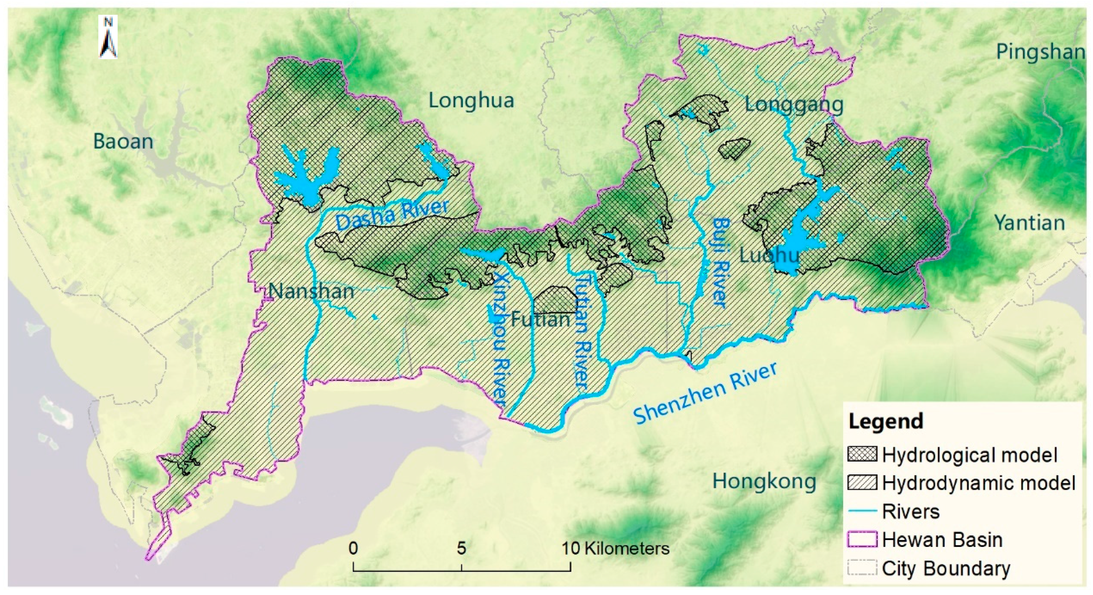
The Shenzhen River and Bay Basin is one of the five major basins in Shenzhen, which has a high hardening surface and short confluence time. In recent years, the damage caused by waterlogging has increased [24]. Heavy rainfall within a short period (approximately 3 h) is the main cause of waterlogging and ponding in urban areas. Therefore, a short heavy rainfall process of 3 h was used as the rainfall scheme in the numerical model to simulate waterlogging. A neural network prediction model for each ponding point was established based on the simulation results. Finally, untrained rainstorm waterlogging samples were used as prediction samples to predict the waterlogging of the ponding point.
2.2. Methods
2.2.1. Construction of Rainfall Schemes
Many types of learning samples are necessary to train neural network models. The larger the training sample size, the more information it contains, and thus, the more intelligent the trained model [25]. Therefore, in this study, a variety of rainfall processes were used as input rainfall conditions to obtain waterlogging samples through numerical model simulations.
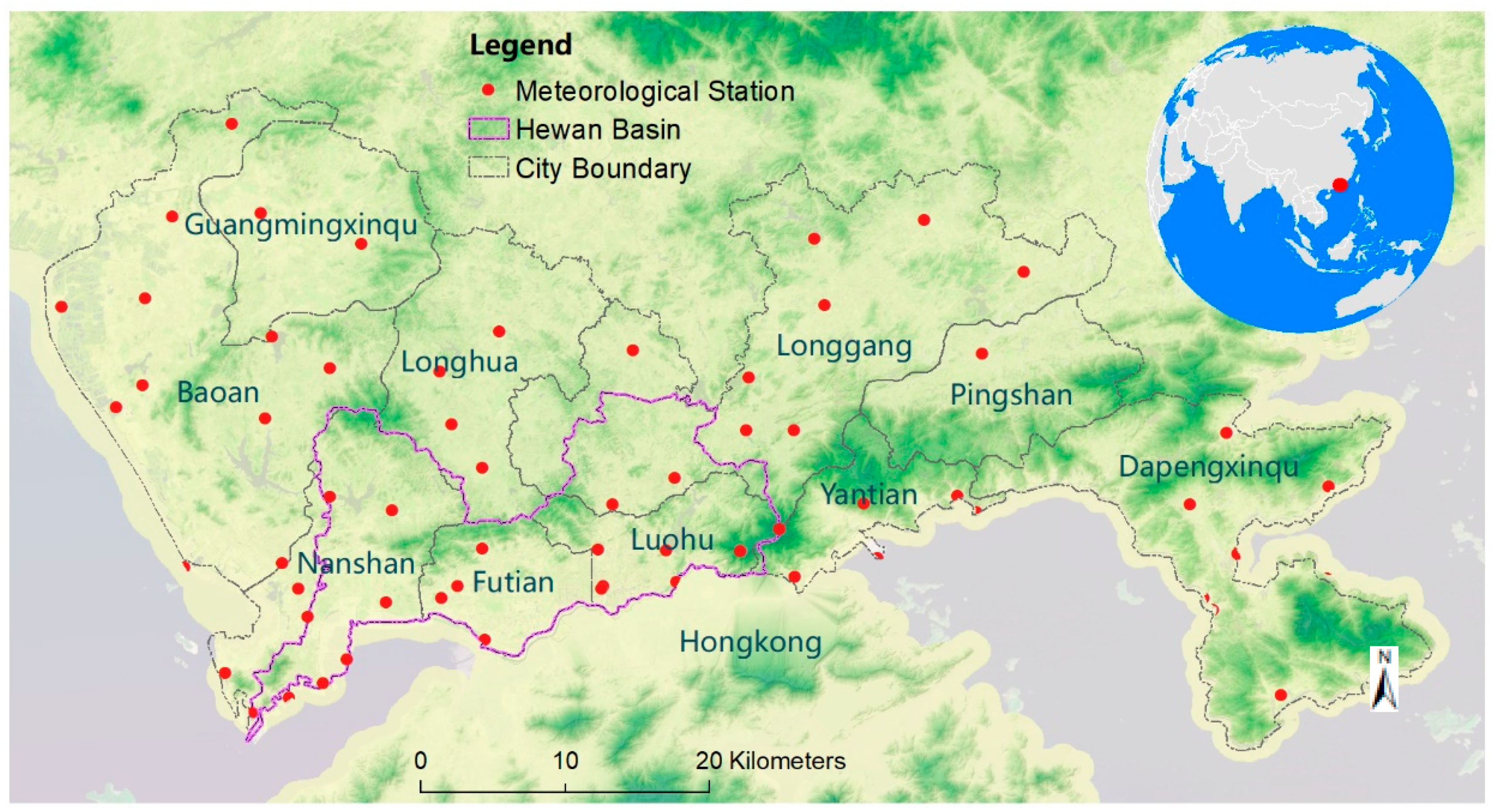
The rainfall scheme mainly included three forms: ① the actual short-duration heavy rainfall process in Shenzhen over 10 years, from 2008 to 2018; ② the designed rainfall process according to the temporal and spatial distribution characteristics of short-duration rainfall; and ③ the design rainfall process with the Chicago rainfall pattern. The study area and distribution of the automated weather stations are shown in Figure 1.
- Actual short-duration heavy rainfallscheme
Based on an analysis of rainfall data from 63 meteorological stations in Shenzhen from 2008 to 2018, 178 short-term rainstorm events [26] occurring within a 3 h rainfall period were selected as the actual rainfall scheme.
- 2.
- Characteristic rainfall schemes with different temporal and spatial distributions
Taking 5 min rainfall data for Shenzhen from 2008 to 2018 as the research object, the temporal and spatial distribution characteristics of rainstorms in Shenzhen were extracted by a machine learning model. The ML (machine learning) model was used to extract the main features from a massive amount of rainstorm samples. First, the rainstorm events were digitized and structured. High-dimensional arrays were established from temporal and spatial dimension perspectives. Dynamic clustering was used to categorize samples describing the temporal and spatial distribution patterns of rainstorms. The centers of rainfall events of each type were extracted to reconstruct the dynamic temporal and spatial distribution patterns of this type of rainfall event.
According to the different temporal and spatial distribution types of rainstorms, the short-duration heavy rainfall process in Shenzhen was divided into three categories. The trajectories of the centroids for the three types of rainfall events are shown in Figure 2, in which different colored points represent rainstorm centers in different periods [26]. In the first type, the rainstorm center moves rapidly from west to southeast within 180 min; in the second type, the rainstorm center moves rapidly from east to west within 180 min; and the third type of rainfall is concentrated, and there is no movement. These three types of characteristic rainfall processes express the temporal and spatial distribution characteristics of short-term heavy rainfall in Shenzhen, of which the first type of rainfall has the highest frequency in the flood season.
Based on these three types of rainfall characteristics, a rainfall process in which the cumulative rainfall at a single station in 3 h ranges from 30–500 mm with 2 mm steps was designed in this study for 708 rainfall events.
- 3.
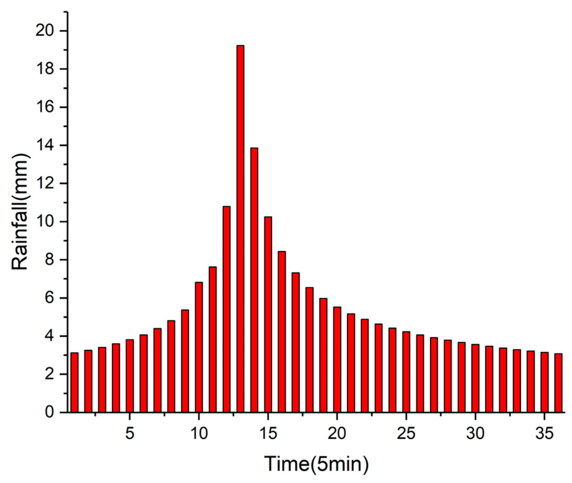
- The rainfall process with the Chicago rainfall pattern
The rainfall process with the Chicago rainfall pattern with 3 h cumulative rainfall at each station from 30–500 mm with 2 mm steps, as shown in Figure 3, was designed for a total of 236 rainfall events.
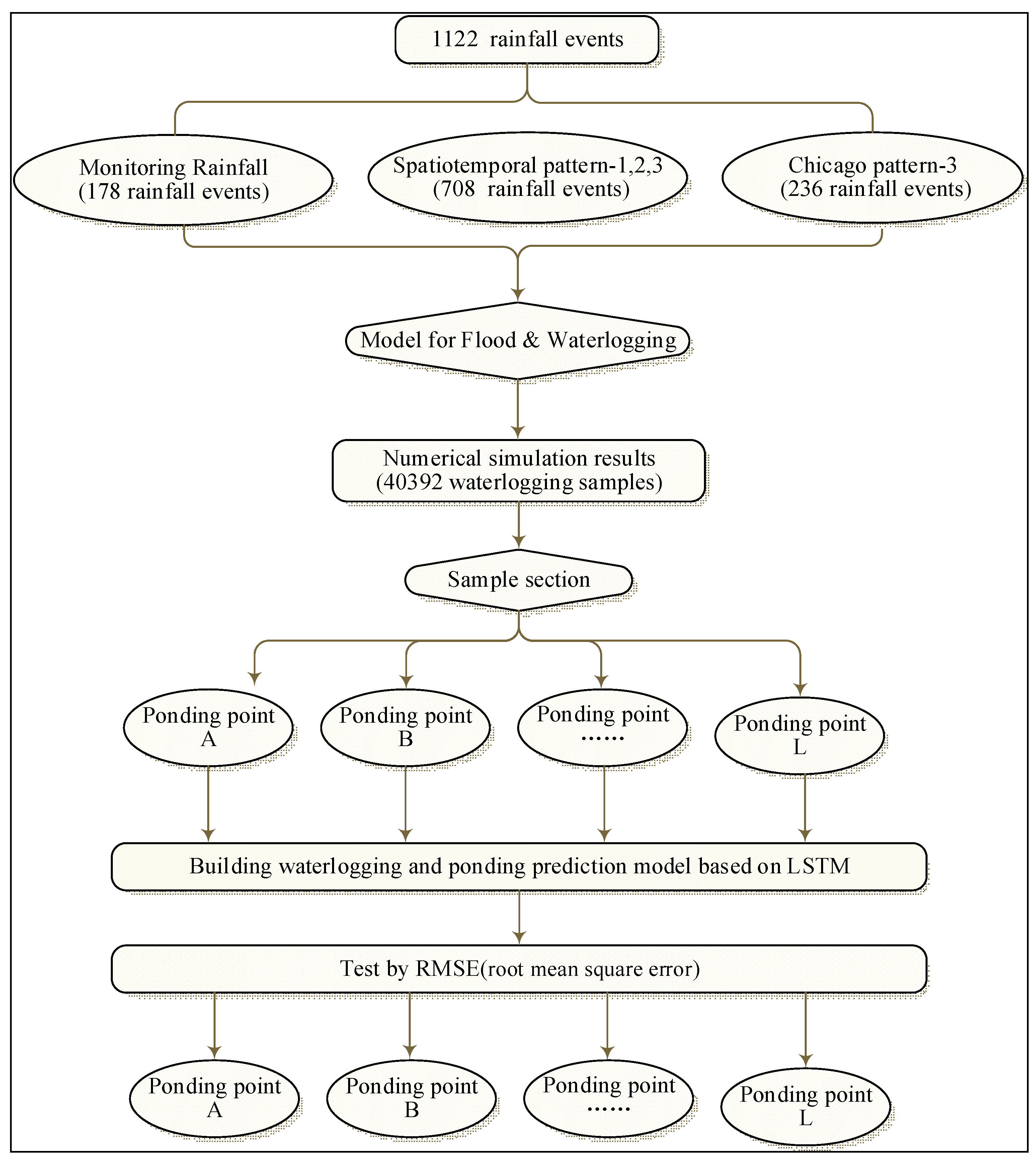
Through these three types of rainfall schemes, a numerical simulation model was used to simulate waterlogging and ponding, and 1122 rainfall events lasting 3 h were calculated. The number and type of samples satisfied the requirements of the neural network model for learning samples. This method is illustrated in Figure 4.
2.2.2. Numerical Simulation Model
With recent advances in technology, the urban flood simulation method has evolved from a simple model to a complex model that combines hydrological and hydrodynamic models with underground pipe network models [27]. In this study, hydrological and hydrodynamic models were established in built-up areas, while only hydrological models were established in non-built-up areas. The coupled model, including the one-dimensional river model, two-dimensional surface model, and an underground pipe network, was established in key areas.
- One dimensional hydrodynamic model of river channel
The flood routing in the study area was simulated by the one-dimensional hydrodynamic model, and its basic control equations are:
Continuity equation:
Energy equation:
where is the cross-section (m2), is section flow (m3/s), is the velocity of lateral confluence (m/s), is time (s), is horizontal coordinates along the flow direction (m), is lateral flow (m2/s), is the water level (m), and is the friction gradient.
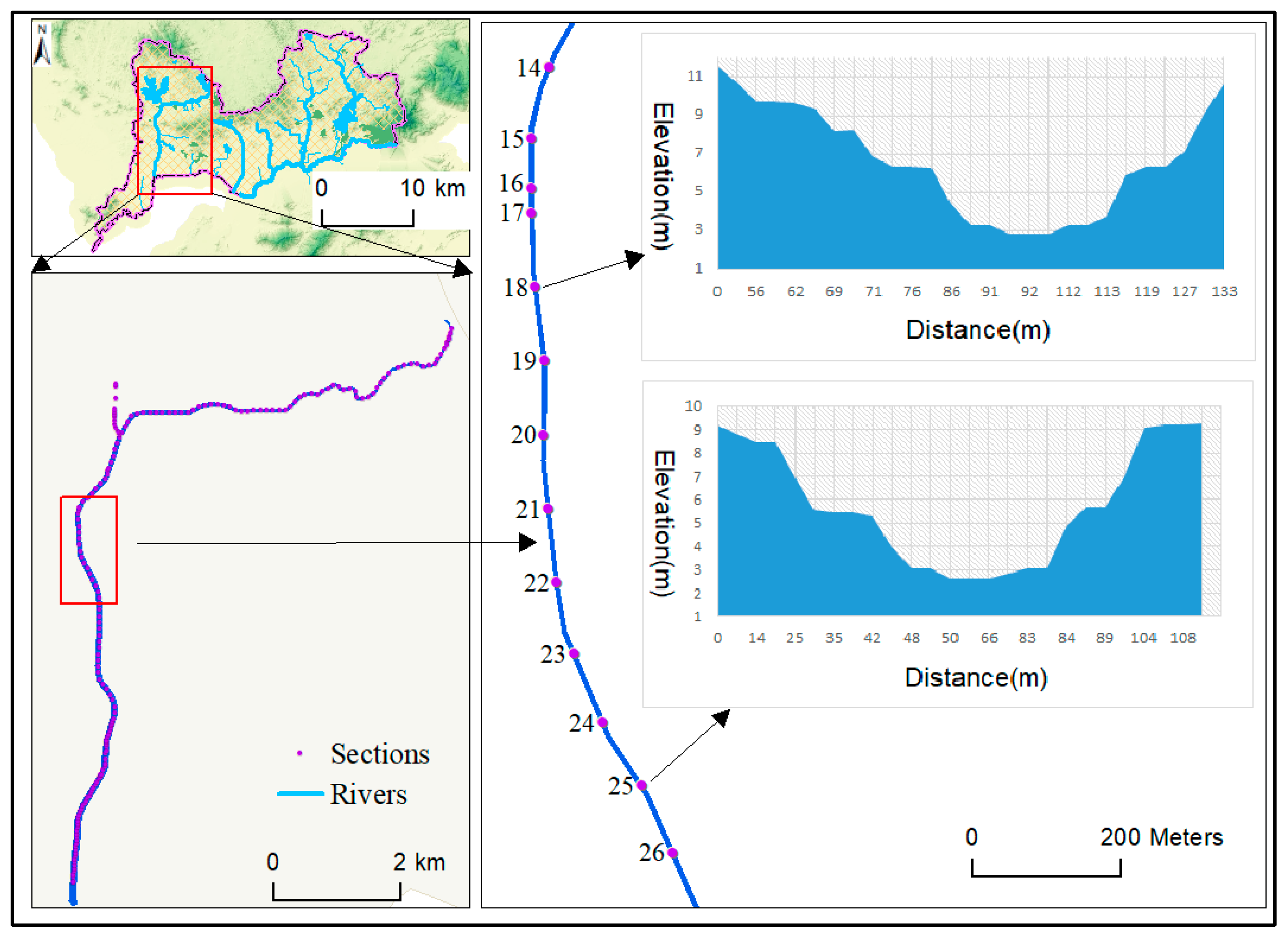
There are 1284 sections in the one-dimensional model in the region, and the distribution and construction range of each section are shown in Figure 5.
- 2.
- Surface runoff model
The continuity equation and momentum equation of the two-dimensional surface hydrodynamic model are as follows:
where is the depth of water (m); is time(s); and are the average vertical unit width discharge in and directions, respectively (m2/s); is the rainfall intensity (m/s); is the water level (m); and and are the average vertical velocity in and directions (m/s).
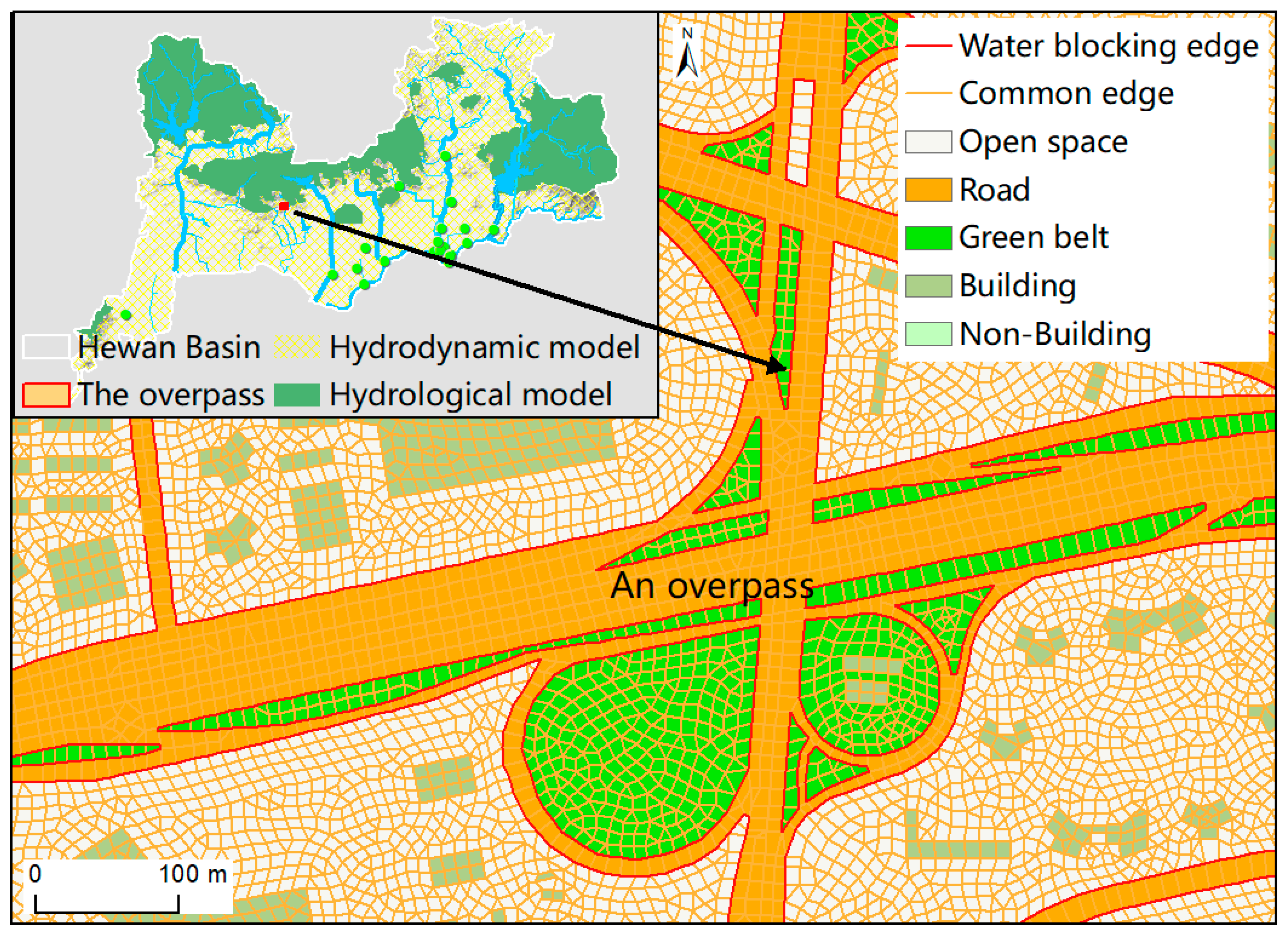
During modeling, the hydrodynamic confluence model is divided by irregular grids with side lengths of 5–10 m. The water-blocking micro-terrain in important areas such as overpasses, roads, water bodies, rivers, railways, communities, bridges, and culverts is the control line. There are a total of 3.04 million grids and 5.64 million sides within the construction scope, with a total simulated area of 226.76 km2, which is shown in Figure 6.
- 3.
- Underground pipe network confluence model
Saint Venant equations combined with the Preissmann virtual slit method [28] were used to establish the underground pipe network confluence model and accurately calculate free surface flow and pressure flow.
The continuity equation is:
The momentum equation is:
where is the water level (m) when there is pressure flow, and is the width of the virtual slit (m).
The details of the coupled model are shown in Figure 7, in which the green area represents the non-built-up area where the hydrological model was built, and the yellow grid area represents the built-up area where the hydrodynamic model was built. The hydrological model calculated the runoff and confluence process of the surface and river network, divided independent hydrological calculation units, and provided inflow profiles for the hydrodynamic model in the built-up area. The two-dimensional hydrodynamic model calculated the water depth and velocity in the surface grid, the one-dimensional model calculated the water level and flow of the river section, and the underground pipe network model calculated the flow and other physical elements in the underground pipe network. These models were coupled according to their three-dimensional urban spatial structures and physical mechanisms.
The one-dimensional river model was coupled with a two-dimensional surface model through a river embankment. The pipe network model was coupled with the one-dimensional model of the river channel through the outlet of the pipe network and with the two-dimensional surface model through the rainwater inlet and drainage outlet. The coupled model not only improved the calculation efficiency but also described and simulated the process of rainfall runoff and waterlogging.
The numerical simulation model has a physical mechanism that describes the production and concentration processes of rainwater on the underlying surface of a city in detail. However, because of the complexity of the model and the large amount of calculation, the calculation time of the 3 h rainfall scheme is more than 18 h, which obviously cannot meet the timeliness requirements of urban risk management. Therefore, it is necessary to select a new technical method to quickly predict urban flood risk.
2.2.3. Training Samples
In this study, a numerical simulation model was used to analyze and calculate the waterlogging and ponding caused by the actual short-duration heavy rainfall process, designed rainfall process characteristics, and the rainfall process with the Chicago rainfall pattern in Shenzhen over a span of 10 years. A total of 1122 rainfall events lasting 3 h and 5 min were obtained, and 40,392 rainstorm waterlogging samples were used to train the network model. The number of training samples met the requirements of the network model.
Intelligent and accurate neural network models require high-quality samples for training. Therefore, in this study, the actual rainfall process was used to check the numerical simulation model to obtain more accurate training samples. The results showed that the accuracy of the numerical model simulation results was high and could satisfy the requirements for the learning sample quality. This study utilized a rainstorm in Shenzhen on 29 August 2018 as an example. A total of 12 ponding points from west to east in the Shenzhen River and Bay Basin were selected to compare the maximum ponding depths of these points between the measured values and model simulation data. The distribution of the ponding points is shown in Figure 8, and the comparison results are presented in Table 1.
As shown in Table 1, the average prediction error between the simulation results and actual measured values of the maximum ponding depth of 12 points was 2.68%, which meets the requirements of the neural network model for the learning sample.
2.2.4. Introduction to LSTM Neural Network Model
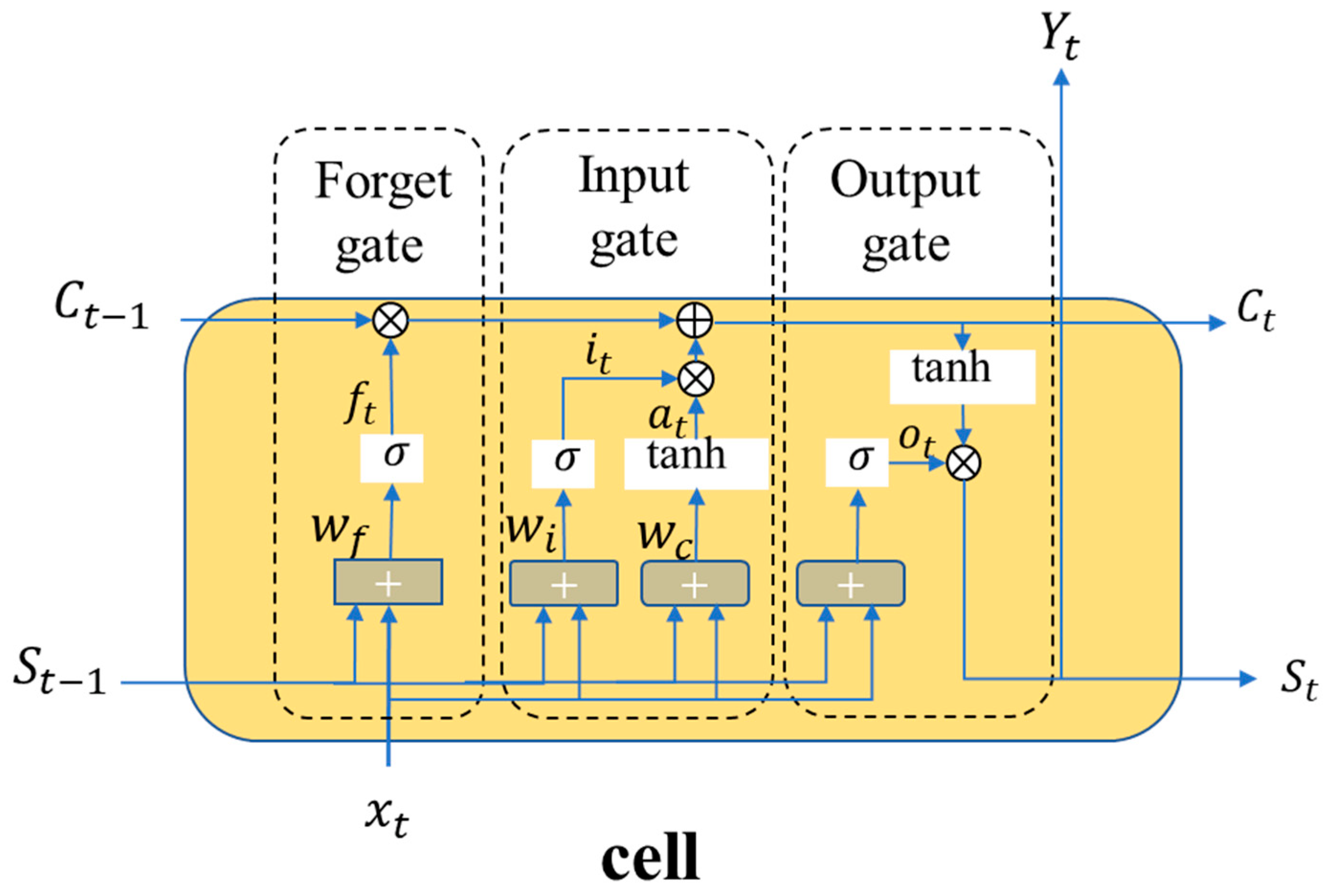
A long short-term memory (LSTM) neural network model is an improved version of the recurrent neural network (RNN) model, which was proposed by Hochreiter and Schmidhuber [29]. Compared with the RNN model, a hidden state Ct and three gates, the forget, input, and output gates, were added to the LSTM model to solve the problem of gradient disappearance or gradient explosion in the RNN model [30]. The structure of the model is shown in Figure 9.
The output of the forget gate is , shown in Equation (8):
where the output of the forget gate is determined by the sample of this time series and the outputs of the previous time’s hidden layer , where is the activation and sigmoid functions. The output of the forget gate represents the probability of forgetting the hidden-cell state of the previous layer. The output of the input gate is shown in Equations (9) and (10), where the activation function in Equation (9) is a sigmoid function, and the activation function in Equation (10) is the tanh function.
is output from and :
where e is the Hadamard product.
The output of the output gate is shown in Equation (12), where the activation function is a sigmoid function:
The output of the hidden layer is the product of the output gate and :
The output result is shown in Equation (14), and the activation function is a sigmoid function:
are all parameters that are iteratively updated by LSTM through the gradient descent method, similar to the RNN algorithm.
2.2.5. Waterlogging and Ponding Prediction Model Based on LSTM
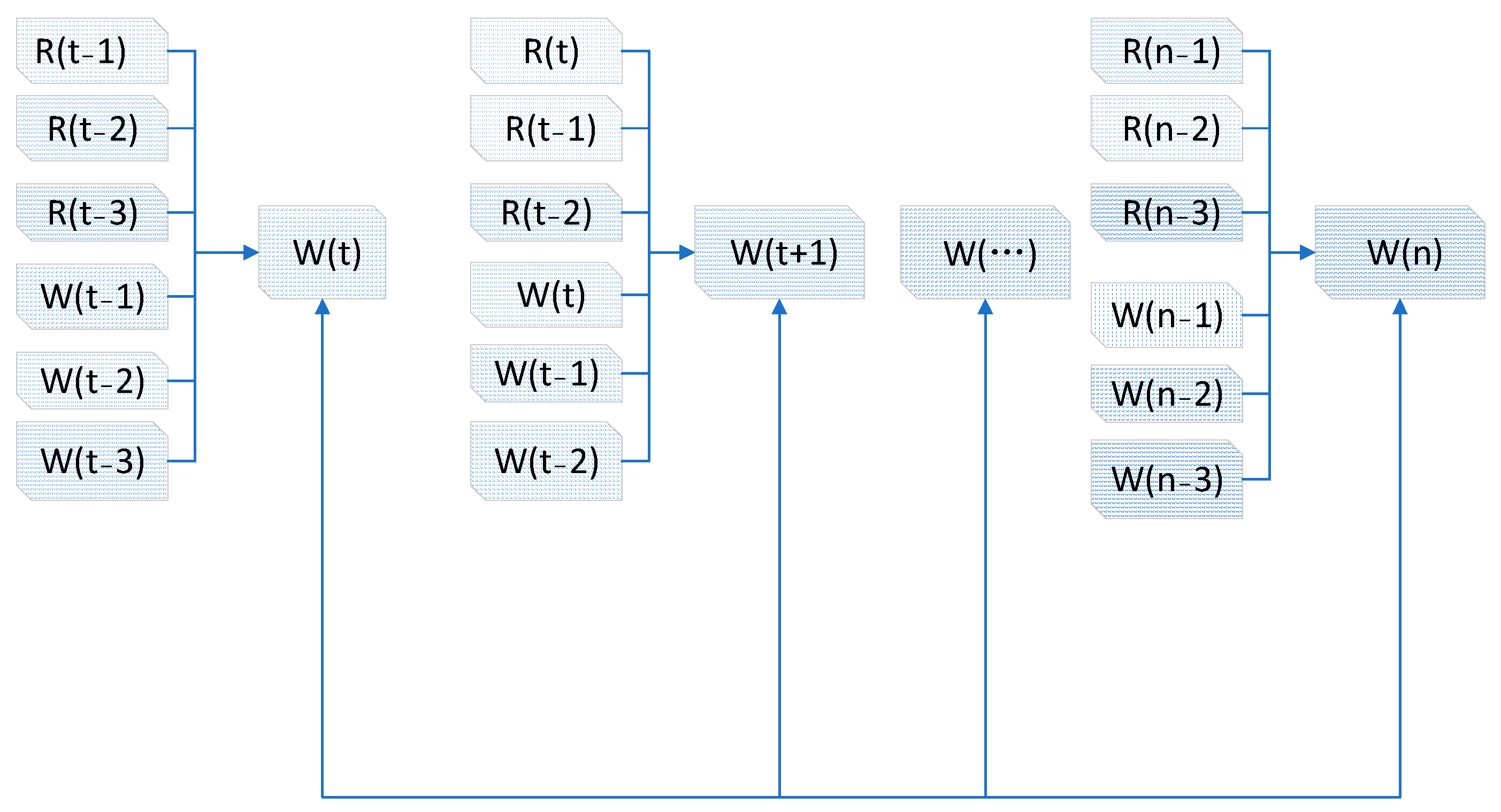
The process of ponding at the ponding point is a continuous time series. The ponding depth of the ponding point is mainly related to the rainfall and the ponding depth in the previous time series. For example, the depth of the ponding point at t has a relationship with the depth of this ponding point at t − 1, t − 2, t − 3, …, and so on. Predicting the ponding depth is a problem of time series prediction. It mainly involves calculating the value of the time series at time t + 1 according to the observation data at the previous times. The LSTM neural network model is suitable for solving the prediction problem of a multi-factor time series. The input value is the historical value, and the output value is the predicted value.
In this study, the 12 waterlogging points in Figure 8 were taken as the research object, and the LSTM neural network prediction model of waterlogging was established with a total of six input factors, as shown in Figure 10.
The output of the LSTM model is the ponding depth of the ponding point at the next time. The future ponding depth was predicted according to the rainfall in the previous time series and ponding depth. Through continuous circulation and training of the model, the ponding depth of each ponding point was predicted for the entire rainfall process. The number of neurons in the input and hidden layers of the model was 50 each. The output y at time Yt was considered the prediction result. Ninety percent of the samples were used as training samples, and the remaining 10% were used as test samples. The rainstorm process without model training was forecasted by using the trained model.
The batch size was 128, the epoch was 300, the loss function was the mean absolute error, and the optimizer was the Adam algorithm. The training results of the model were evaluated by calculating the root mean square error between the predicted and real data. The results showed that the error of the LSTM prediction model decreased rapidly when the training time was approximately 100. When the training time was approximately 120, the error curve reached an inflection point, the error decline speed tended to be gentle, and the model gradually converged. This shows that the LSTM neural network algorithm selected in this study is reasonable and that the data sample quality of the training model is reliable.
3. Results and Discussion
Using 12 points (points A–L) from west to east in the Shenzhen River and Bay Basin (Figure 8) as the analysis object, the rainfall process without training was input into the numerical simulation model and the trained LSTM neural network to predict the ponding depth. The input rainfall was 6 h at 5 min intervals. The first 3 h was the design rainfall process with the Chicago and characteristic rain types, and there was no rainfall in the last 3 h to completely simulate the rain–waterlogging–recession process. To compare the calculation results of the two models more intuitively, process lines of the prediction results of the numerical and neural network models were constructed. The similarity between the two curves was determined by the determination coefficient R2. The closer the determination coefficient R2 is to 1, the higher the fitting degree of the two curves.
The rainfall process in which the rainstorm center moves from west to east is the characteristic rainfall process with the highest frequency in the study area. Owing to space limitations, in this study, the simulation results of this type of characteristic rainfall process and the rainfall process with the Chicago rainfall pattern were analyzed and compared. The prediction results of these two models are shown in Figure 11 and Figure 12.
As shown in Figure 11 and Figure 12, the numerical and LSTM models could simulate and predict the ponding process of each ponding point under different rainfall conditions. Moreover, the fitting error of the simulation results of the two models was very small, and the determination coefficient, R2, was greater than 0.85.
The simulation results of rainfall schemes with the Chicago rainfall pattern are shown in Figure 11. Due to the similar shape of the rainfall patterns, the ponding depth change curves of the 12 ponding points from points A–L, which were distributed in the west, middle, and east of the area, as well as the occurrence times of the maximum ponding depth and retreat time, were also similar.
The simulation results of the rainfall schemes moving from west to east are shown in Figure 12. This type of rainfall is the most frequent during the flood season in the Shenzhen River and Bay Basin. The characteristics of the temporal and spatial distribution of this type are that the rainstorm center moves from the west to the east within 180 min, the rain in the west and central regions is flat with a small amount of rainfall, and rainfall in the northeast and eastern regions is concentrated, with a large amount of rainfall in the northeast.
The change in ponding depth of the 12 ponding points, points A–L in Figure 12, reflects the movement of the rainfall peak. The rainfall peak in the western region occurred within the first 30 min after rainfall, and the water accumulation points A and B in the western region reached the maximum water accumulation depth within the first hour. The rainfall peak in the middle region occurred approximately 1 h after the rainfall process, and the ponding points C, D, and E in the middle region reached the maximum ponding depth 1.5–2 h after the beginning of rainfall. The rainfall peak in the northeast region occurred approximately 2 h after the beginning of rainfall, and the ponding points F, G, and H reached the maximum ponding depth approximately 2.5 h after the beginning of rainfall. In addition, the maximum ponding depth of the I–L ponding points reached the maximum ponding depth 3 h after rainfall. For different regions, the peak time of ponding depth varies, and this key time point is very important for urban waterlogging prediction and early warning.
It can also be seen in Figure 12 that the shape of the rainfall pattern had a direct impact on the shape of the water process curve at the ponding point. The gentler the rainfall, the gentler the ponding curve corresponding to the ponding point; the more concentrated the rainfall, the more concentrated the ponding curve.
The numerical simulation model used in this study and the neural network model trained based on the simulation results of the numerical model reflect the relationship between the change in ponding depth and temporal and spatial changes in rainfall. The prediction results were reasonable and reliable and could simulate and predict the change in ponding depth at ponding points under different rainfall conditions.
Due to the influence of natural environmental factors, the continuity of the measured data was poor; therefore, only the measured maximum ponding depth was compared. The results of the numerical and LSTM models were compared with the measured maximum ponding depth from heavy rain in Shenzhen on 29 August 2018, without training, and the results are shown in Table 2.
As shown in Table 2, the average error between the maximum ponding depths simulated by the numerical model and the measured values was 2.68%, while the error between the maximum ponding depths simulated by the LSTM neural network model and the measured values was 3.05%. The prediction error increased by 0.37% between the two models, mainly because the neural network model was trained based on the numerical simulation results, leading to error accumulation in the predicted results.
When calculating the same rainfall scheme for 3 h rainfall, the LSTM model required only 0.2 s, while the numerical model required 18 h, with a 324,000-times increase in calculation speed. The computational time of the numerical model increased linearly with the size of the grid. If the computational range is expanded, the computational efficiency will not meet the application requirements. The prediction time of hundreds of ponding points with the LSTM model was maintained at the scale of minutes, which greatly reduces the calculation time and can effectively meet emergency needs.
4. Conclusions
In this study, a “double models” method was established by combining a numerical simulation model and an artificial neural network. Through the numerical simulation model, numerous rainstorm waterlogging samples were generated under different rainfall conditions, and the LSTM neural network model was trained using this sample. The trained LSTM neural network model could quickly predict the ponding situation.
Compared with the actual measured values, the predicted values of the numerical and LSTM prediction models had a small average error and high prediction accuracy. The average error of the prediction value of the numerical model was 2.68%, while that of the LSTM neural network model was 3.05%, with a 0.37% increase in that of LSTM. However, as the neural network model was trained based on the numerical simulation results, the prediction result errors accumulated. However, as shown in Table 2, the standard deviation of the LSTM model error was only 1.08, indicating that the prediction error of the LSTM model was more concentrated.
The simulation speed of the “double models” method was 324,000 times that of the traditional numerical model. If the computing area is expanded, the efficiency advantage of the LSTM neural network trained by the numerical model will be more evident at large and high-density scales.
The “double models” prediction method combining a numerical simulation model and AI technology proposed in this study not only addresses the low calculation efficiency of the numerical simulation model but also meets the demands of AI technology for numerous training samples. In addition, the proposed method has a fast calculation speed and high accuracy. This provides a new idea for the application of AI technology in the field of disaster prevention and reduction.
The input factors of the simulation model presented in this paper are the ponding depth and rainfall of the previous time series, and the rainfall refers to the rainfall caused by any weather system, which is independent of the weather system causing the rainfall. Any weather system that produces rainfall and waterlogging can be predicted by the model described in this paper. This paper only puts forward the method of forecasting rainstorms and waterlogging. This method still has many shortcomings and deficiencies. With the development of technology and the improvement of data samples, this method will gradually mature and can be integrated into the early warning system. Moreover, as the AI model is updated and improved, the requirements of AI technology for samples will be gradually reduced, and the prediction accuracy will be greatly improved.
Author Contributions
Y.L. (Yesen Liu) and J.Z. collected and processed the data, Y.L. (Yuanyuan Liu), F.C. and H.R. proposed the model and analyzed the results, and Y.L. (Yuanyuan Liu) and Y.L. (Yesen Liu) wrote the manuscript. All authors have read and agreed to the published version of the manuscript.
Funding
This work was supported by the National Natural Science Foundation of China (Grant No. 41822104).
Institutional Review Board Statement
Not applicable for studies not involving humans or animals.
Informed Consent Statement
Not applicable.
Data Availability Statement
Participants of this study did not agree for their data to be shared publicly, so supporting data is not available.
Conflicts of Interest
The authors declare no conflict of interest.
References
- Tingsanchali, T. Urban flood disaster management. Procedia Eng. 2012, 32, 25–37. [Google Scholar] [CrossRef] [Green Version]
- Huang, H.; Xi, C.; Zhu, Z.; Xie, Y.; Kai, L. The changing pattern of urban flooding in Guangzhou, China. Sci. Total Environ. 2017, 622–623, 394. [Google Scholar] [CrossRef] [PubMed]
- Jha, A.; Lamond, J.; Proverbs, D.; Bhattacharya-Mis, N.; Barker, R. Cities and Flooding: A Guide to Integrated Urban Flood Risk Management for the 21st Century; World Bank Publications: Washington, DC, USA, 2012. [Google Scholar]
- Cheng, X.T. Urban Water Disasters and Strategy of Comprehensive Control of Water Disaster. J. Catastrophol. 2010, 25, 10–15. [Google Scholar]
- Seyoum, S.D.; Vojinovic, Z.; Price, R.K.; Weesakul, S. Coupled 1D and Noninertia 2D Flood Inundation Model for Simulation of Urban Flooding. J. Hydraul. Eng. 2012, 138, 23–34. [Google Scholar] [CrossRef]
- Zhou, H.-L.; Chen, Y.-B. 2D shallow-water simulation for urbanized areas. Adv. Water Sci. 2011, 22, 407–412. [Google Scholar]
- Guo, K.H.; Guan, M.F.; Yu, D.P. Urban surface water flood modelling: A comprehensive review of current models and future challenges. Hydrol. Earth Syst. Sci. 2021, 25, 2843–2860. [Google Scholar] [CrossRef]
- Zhang, H.P.; Wu, W.M.; Hu, C.H.; Hu, C.; Li, M.; Hao, X.; Liu, S. A distributed hydrodynamic model for urban storm flood risk assessment. J. Hydrol. 2021, 600, 126513. [Google Scholar] [CrossRef]
- DHI. MIKE 1D, DHI Simulation Engine for 1D River and Urban Modelling; DHI: Singapore, 2012. [Google Scholar]
- DHI. MIKE 21 Flow Model FM, Hydrodynamic and Transport Module, Scientific Documentation; DHI: Singapore, 2007. [Google Scholar]
- Rangari, V.A.; Umamahesh, N.V.; Bhatt, C.M. Assessment of inundation risk in urban floods using HEC RAS 2-D. Model. Earth Syst. Environ. 2019, 5, 1839–1851. [Google Scholar] [CrossRef]
- Huang, G.; Chen, W.; Yu, H. Construction and evaluation of an integrated hydrological and hydrodynamics urban flood model. Adv. Water Sci. 2021, 32, 334–344. [Google Scholar]
- Jiang, C.; Zhou, Q.; Yu, W.; Yang, C.; Lin, B. A dynamic bidirectional coupled surface flow model for flood inundation simulation. Nat. Hazards Earth Syst. Sci. 2021, 21, 497–515. [Google Scholar] [CrossRef]
- Hu, C.; Xia, J.; She, D.X.; Song, Z.; Zhang, Y.; Hong, S. A new urban hydrological model considering various land covers for flood simulation. J. Hydrol. 2021, 603, 126833. [Google Scholar] [CrossRef]
- Soares-Frazao, S.; Lhomme, J.; Guinot, V.; Zech, Y. Two-dimensional shallow-water model with porosity for urban flood modelling. J. Hydraul. Res. 2008, 46, 45–64. [Google Scholar] [CrossRef]
- Lecun, Y.; Bengio, Y.; Hinton, G. Deep learning. Nature 2015, 521, 436. [Google Scholar] [CrossRef] [PubMed]
- Meer, P.; Mintz, D.; Rosenfeld, A.; Dong, Y.K. Robust regression methods for computer vision: A review. Int. J. Comput. Vis. 1991, 6, 59–70. [Google Scholar] [CrossRef]
- Sundermeyer, M.; Schlüter, R.; Ney, H. LSTM Neural Networks for Language Modeling. In Proceedings of the Interspeech, Portland, OR, USA, 9–13 September 2012. [Google Scholar]
- Liu, Y.Y.; Li, L.; Zhang, W.H.; Chan, P.W.; Liu, Y.S. Rapid identification of rainstorm disaster risks based on an artificial intelligence technology using the 2DPCA method. Atmos. Res. 2019, 227, 157–164. [Google Scholar] [CrossRef]
- Qing, L.; Hai-tao, X.; Jun-liang, Y. Daily Water Volume Prediction Algorithm of Urban Smart Water Based on Big Data. J. Beijing Univ. Posts Telecommun. 2021, 44, 82–88. [Google Scholar]
- Barzegar, R.; Aalami, M.T.; Adamowski, J.F. Coupling a Hybrid CNN-LSTM Deep Learning Model with a Boundary Corrected Maximal Overlap Discrete Wavelet Transform for Multiscale Lake Water Level Forecasting. J. Hydrol. 2021, 598, 126196. [Google Scholar] [CrossRef]
- Xinjun, W.; Xiaodong, Z.; Xi, D.; Zhentao, X.; Cheng, Q. CNN flood routing method based on data-driven training. J. Hydroelectr. Eng. 2021, 40, 8. [Google Scholar]
- Ganggang, B.; Jingming, H.; Hao, H.; Junqiang, X.; Bingyao, L. Intelligent monitoring method for road inundation based on deep learning. Water Resour. Prot. 2021, 37, 6. [Google Scholar]
- Gao, X.; Liu, J. Effect of Urbanization on River Hydrological Process in Shenzhen River Basin. Acta Sci. Nat. Univ. Pekin. 2012, 48, 153–159. [Google Scholar]
- Liu, Y.-Y.; Li, Z.; Lei, L.; Yesen, L. Storm surge nowcasting based on multivariable LSTM neural network model. Mar. Sci. Bull. 2020, 39, 689–694. [Google Scholar]
- Liu, Y.-Y.; Li, L.; Liu, Y.-S.; Chan, P.W.; Zhang, W.-H. Dynamic spatial-temporal precipitation distribution models for short-duration rainstorms in Shenzhen, China based on machine learning. Atmos. Res. 2020, 237, 104861. [Google Scholar] [CrossRef]
- Leandro, J.; Chen, A.S.; Djordjevic, S.; Savic, D.A. Comparison of 1D/1D and 1D/2D Coupled (Sewer/Surface) Hydraulic Models for Urban Flood Simulation. J. Hydraul. Eng. 2009, 135, 495–504. [Google Scholar] [CrossRef]
- Preissmann, A.; Cunge, J.A. Calcul des intumeseences sur machines electroniques. In Proceedings of the Ninth Convention of the International Association for Hydraulic Research, Dubrovnik, Croatia, 4–7 September 1961. [Google Scholar]
- Hochreiter, S.; Schmidhuber, J. Long Short-Term Memory. Neural Comput. 1997, 9, 1735–1780. [Google Scholar] [CrossRef] [PubMed]
- Schmidhuber, J.; Gers, F.; Eck, D. Learning Nonregular Languages: A Comparison of Simple Recurrent Networks and LSTM. Neural Comput. 2014, 14, 2039–2041. [Google Scholar] [CrossRef] [PubMed]
Figure 1.
Study area and distribution of the automated weather stations.

Figure 2.
Distribution map of rainstorm center points in various rainfall periods.

Figure 3.
Chicago rainfall pattern.

Figure 4.
Sketch map of the method for creating the numerical simulation model.

Figure 5.
Distribution map of river section.

Figure 6.
Mesh of 2D model.

Figure 7.
Distribution map of hydrological and hydrodynamic models.

Figure 8.
Distribution of ponding points. (Number of A–L for waterlogging point).

Figure 9.
Structure diagram of a long short-term memory neural network model.

Figure 10.
Factors related to prediction of ponding.

Figure 11.
Simulation results of rainfall scheme with the Chicago rainfall pattern.

Figure 12.
Simulation results of rainfall schemes moving from west to east.


Table 1.
Comparison of maximum ponding depths of measured values and simulated results at waterlogging points during a heavy rainstorm in Shenzhen on 29 August 2018.
Table 1.
Comparison of maximum ponding depths of measured values and simulated results at waterlogging points during a heavy rainstorm in Shenzhen on 29 August 2018.
| Serial Number | Waterlogging Point | Maximum Ponding Depth, Measured Values (cm) | Maximum Ponding Depth, Simulation Results (cm) | Error (%) |
|---|---|---|---|---|
| 1 | Point A | 40 | 39.8 | 0.50 |
| 2 | Point B | 50 | 47 | 6.00 |
| 3 | Point C | 30 | 29.3 | 2.33 |
| 4 | Point D | 25 | 24.2 | 3.20 |
| 5 | Point E | 40 | 42.9 | 7.25 |
| 6 | Point F | 48 | 46.9 | 2.29 |
| 7 | Point G | 55 | 56.1 | 2.00 |
| 8 | Point H | 35 | 34.9 | 0.29 |
| 9 | Point I | 55 | 54.5 | 0.91 |
| 10 | Point J | 50 | 49.7 | 0.60 |
| 11 | Point K | 15 | 14.8 | 1.33 |
| 12 | Point L | 20 | 18.9 | 5.50 |
| Average error | 2.68 |
Table 2.
Comparison between the maximum ponding depths predicted by the numerical model and long short-term memory (LSTM) model and the measured values.
Table 2.
Comparison between the maximum ponding depths predicted by the numerical model and long short-term memory (LSTM) model and the measured values.
| Serial Number | Waterlogging Point | Measured Values (cm) | Numerical Model Results (cm) | Error with Numerical Model (%) | LSTM Results (cm) | Error with LSTM (%) |
|---|---|---|---|---|---|---|
| 1 | Point A | 40 | 39.8 | 0.50 | 39.2 | 2.00 |
| 2 | Point B | 50 | 47 | 6.00 | 51.2 | 2.40 |
| 3 | Point C | 30 | 29.3 | 2.33 | 28.3 | 5.67 |
| 4 | Point D | 25 | 24.2 | 3.20 | 23.5 | 6.00 |
| 5 | Point E | 40 | 42.9 | 7.25 | 41.2 | 3.00 |
| 6 | Point F | 48 | 46.9 | 2.29 | 46.9 | 2.29 |
| 7 | Point G | 55 | 56.1 | 2.00 | 56.1 | 2.00 |
| 8 | Point H | 35 | 34.9 | 0.29 | 35.7 | 2.00 |
| 9 | Point I | 55 | 54.5 | 0.91 | 55.2 | 0.36 |
| 10 | Point J | 50 | 49.7 | 0.60 | 50.7 | 1.40 |
| 11 | Point K | 15 | 14.8 | 1.33 | 15.9 | 6.00 |
| 12 | Point L | 20 | 18.9 | 5.50 | 19.3 | 3.50 |
| Average error | 2.68 | 3.05 | ||||
| Standard deviations of errors | 2.25 | 1.80 | ||||
Publisher’s Note: MDPI stays neutral with regard to jurisdictional claims in published maps and institutional affiliations. |
© 2022 by the authors. Licensee MDPI, Basel, Switzerland. This article is an open access article distributed under the terms and conditions of the Creative Commons Attribution (CC BY) license (https://creativecommons.org/licenses/by/4.0/).
Share and Cite
MDPI and ACS Style
Liu, Y.; Liu, Y.; Zheng, J.; Chai, F.; Ren, H. Intelligent Prediction Method for Waterlogging Risk Based on AI and Numerical Model. Water 2022, 14, 2282. https://doi.org/10.3390/w14152282
AMA Style
Liu Y, Liu Y, Zheng J, Chai F, Ren H. Intelligent Prediction Method for Waterlogging Risk Based on AI and Numerical Model. Water. 2022; 14(15):2282. https://doi.org/10.3390/w14152282
Chicago/Turabian StyleLiu, Yuanyuan, Yesen Liu, Jingwei Zheng, Fuxin Chai, and Hancheng Ren. 2022. "Intelligent Prediction Method for Waterlogging Risk Based on AI and Numerical Model" Water 14, no. 15: 2282. https://doi.org/10.3390/w14152282
Note that from the first issue of 2016, this journal uses article numbers instead of page numbers. See further details here.