
Spatiotemporal Variation and Driving Factors of Water Supply Services in the Three Gorges Reservoir Area of China Based on Supply-Demand Balance


1
Research Center for Economy of Upper Reaches of the Yangtze River, Chongqing Technology and Business University, Chongqing 400067, China
2
School of Economics, Chongqing Technology and Business University, Chongqing 400067, China
3
School of Economics, Yunnan University, Kunming 650091, China
*
Author to whom correspondence should be addressed.
†
These authors contributed equally to this work.
Water 2022, 14(14), 2271; https://doi.org/10.3390/w14142271
Submission received: 9 June 2022
/
Revised: 16 July 2022
/
Accepted: 19 July 2022
/
Published: 21 July 2022
(This article belongs to the Special Issue Optimization and Prediction of Water Quality Model Based on Artificial Intelligence)
Abstract
:Water supply services (WSSs) are critical to human survival and development. The Integrated Valuation of Ecosystem Services and Trade-offs (InVEST) model enables an integrated, dynamic, and visual assessment of ecosystem services at different scales. In addition, Geodetector is an effective tool for identifying the main driving factors of spatial heterogeneity of ecosystem services. Therefore, this article takes the Three Gorges Reservoir Area (TGRA), the most prominent strategic reserve of freshwater resources in China, as the study area and uses the InVEST model to simulate the spatiotemporal heterogeneity of the supply-demand balance of WSSs and freshwater security patterns in 2005, 2010, 2015, and 2018, and explores the key driving factors of freshwater security index (FSI) with Geodetector. The total supply of WSSs in the TGRA decreased by 1.05% overall between 2005 and 2018, with the head and tail areas being low-value regions for water yield and the central part of the belly areas being high-value regions for water yield. The total demand for WSSs in the TGRA increased by 9.1%, with the tail zones and the central part of the belly zones being the high water consumption areas. In contrast, the head zones are of low water consumption. The multi-year average FSI of the TGRA is 0.12, 0.1, 0.21, and 0.16, showing an upward trend. The key ecological function areas in the TGRA are high-value FSI regions, while the tail zones in the key development areas are low-value FSI regions. Industrial water consumption significantly impacts FSI, with a multi-year average q value of 0.82. Meanwhile, the q value of industrial and domestic water consumption on FSI in 2018 increased by 43.54% and 30%, respectively, compared with 2005. This study analyzes the spatiotemporal variation of WSSs and detects the drivers in the natural-economic-social perspective and innovation in ecosystem services research. The study results can guide water resource security management in other large reservoirs or specific reservoir areas.
1. Introduction
Ecosystems provide a range of goods or services that satisfy human production and livelihoods, known as ecosystem services (ESs) [1,2]. The Millennium Ecosystem Assessment (MA) classifies ESs into four broad categories: provisioning, regulating, supporting, and cultural services [3]. Because ESs can characterize elements and functions of ecosystems, they have become essential indicators for studying ecological and environmental issues [4]. However, ESs are influenced by both natural and socioeconomic factors [5,6]. With continued socioeconomic development and rapid urbanization, the cumulative demand of human society will undoubtedly increase in the future [7], which will eventually lead to the contradiction between limited natural resources and unlimited human demand, posing a considerable challenge to ecosystem conservation [8]. Therefore, it is necessary to explore the coordination between the supply and demand of ESs and to precisely plan interventions and policies for ESs supply and demand, which is essential for balancing economic development with ecological conservation and achieving regional ecological security and sustainable development [9].
Water plays a crucial role in maintaining the balance of watershed ecosystems and the sustainability of ecological carrying capacity [10]. Human activity is inseparable from its supply and constantly influences water resource evolution and cyclical processes [11]. Water research mainly covers water quality [12], quantity [13], or its associated impacts [14]. Water supply services (WSSs) are the storage and retention of water by ecosystems, which are vital services in watershed ecosystems [15] and play a crucial role in the water balance of watersheds and human survival and development [16]. Since the 1990s, WSSs have become a hot topic of research in watershed management [17,18]. Previously, the assessment of ESs was mainly based on land use types and combined with factor analysis [19]. However, the results were from the lack of spatial concepts, single evaluation, and preliminary dynamic studies [20]. In recent years, with the development of remote sensing and GIS technology, some researchers have started to conduct ecosystem service studies with the help of spatial analysis models, which have become a breakthrough in solving the above problems [21]. The Integrated Valuation of Ecosystem Services and Trade-offs (InVEST) model is the most widely used. Most studies adopt the model modules to assess the relevant ecosystem services, analyze the spatial management pattern, and make management plans. For example, Benra et al. [22] used the InVEST seasonal water yield model to assess the water monitoring performance of 224 catchments in southern Chile, helping inform water supply policy decisions. Liu et al. [23] utilized the InVEST annual water yield model to estimate the water supply of the Beijing Zhangcheng district ecosystem and quantitatively analyzed the characteristics of the spatiotemporal distribution of WSSs in the watershed and the influence of different topographic factors, which is conducive to formulating water conservation region protection and establishing ecological compensation mechanisms. Bejagam et al. [24] used the InVEST annual water yield model to analyze the impacts of climate change on water supply and water-associated services such as hydropower generation in the densely populated Tungabhadra Basin. Their research has found that water provision services in the Tungabhadra basin are vulnerable to climate change. Emlaei et al. [25] applied the InVEST annual water yield model to analyze the water supply in the Haraz Basin. Their study also explored the combined effects of land use/cover and climate change on the short and long-term water supply to provide a reference for implementing reasonable land management strategies to improve water production under climate change. Therefore, in conjunction with the above research, the InVEST model is an effective tool for assessing natural capital and spatial analysis that can inform management decision making. However, most of these studies focus on the quantitative assessments of supply. With economic development and population growth, supply alone is a limited guide to future water security and conservation measures [26]. The quantification of demand for WSSs has been conducted in recent years, first by Kroll et al. [27] for the Leipzig region and later by Boithias et al. [28] who clearly show that the demand for WSSs can be characterized by the total amount of water for agriculture, industry, and domestic consumption. Various scholars have recently explored methods and case applications for quantifying the demand for ecosystem services. Azlan et al. [29] have used a fuzzy inference system to quantify water demand at Kenyir Lake, Malaysia, to provide more promising results for sustainable local water demand management. Xu et al. [30] further investigated the supply and demand of water resources in the Ningxia region of China. Integrating the flow of ecosystem services with inter-regional ecological compensation provides a spatial visualization reference for water resource governance for policymakers.
In summary, many scholars have conducted research on WSSs. Nevertheless, there is less research on the demand for WSSs and the different categories of driving factors. Currently, most studies on WSSs have focused on the amount of supply [31] or the influence of natural factors on the supply of WSSs [32,33]. This article will, therefore, aim to assess the supply and demand for WSSs by combining natural ecological and human social needs. Based on quantified supply and demand, the article will explore the various drivers of WSSs under the natural-economic-social category, which is an exploration and attempt. Meanwhile, regarding spatial scale, studies on WSSs have been conducted on an enormous scope, such as watersheds [34] and states [35]. Nevertheless, there is less research on WSSs at the county scale. Since counties are the most basic administrative units in China, and the scope of national planning and actual investment in ecological protection projects are all based on counties [36], the importance of which is self-evident, it is necessary to discuss WSSs at the county scale. Therefore, this article will explore the WSSs from a county perspective which can more intuitively reflect the situation in different administrative units and give policy recommendations tailored to local conditions.
The Three Gorges Reservoir Area (TGRA) is the most significant strategic reserve of freshwater resources in China, sustaining 35% of China’s freshwater resources and the drinking water security of more than 300 million people in the middle and lower reaches of the Yangtze River [37]. The TGRA is considered the most important ecological corridor and eco-economic zone in the Yangtze River basin [38]. Its freshwater security directly affects the Yangtze River basin’s ecological security and sustainable socio-economic development. Current studies on the TGRA have focused on the subsidence zone [39], migration [40], and geological hazards [41]. However, there is still a lack of studies on WSSs in the TGRA, especially on the water quantity from ecosystem services. To fully understand and give full play to the WSSs function of the TGRA and actively maintain freshwater security, it is essential to study the spatial and temporal variations of the supply-demand balance of WSSs from the country scale.
In this study, from the perspective of the “ecology-economy-society” composite ecosystem, firstly, the InVEST annual water yield model was used to assess the supply changes of WSSs in the TGRA using four periods of remote sensing data from 2005, 2010, 2015, and 2018. Integrating the remote sensing data, GIS technology, and ecosystem service assessment efficiently extracted the characteristics of regional ecological disturbance and restoration. This improves the accuracy of spatiotemporal dynamic simulation of WSSs, which is innovative and practical in research methods and ideas. Secondly, socio-economic data are introduced to analyze the demand for WSSs. Then the supply and demand are matched with the corresponding administrative regions to investigate the spatial and temporal changes in the supply and demand balance of WSSs and freshwater security index (FSI) in each administrative region of the TGRA. Finally, the driving factors of FSI are analyzed by Geodetector to provide a scientific basis and reference for improving freshwater resource management in the TGRA, realizing rational allocation of freshwater resources, and ensuring regional freshwater security.
2. Data and Methods
2.1. Study Area
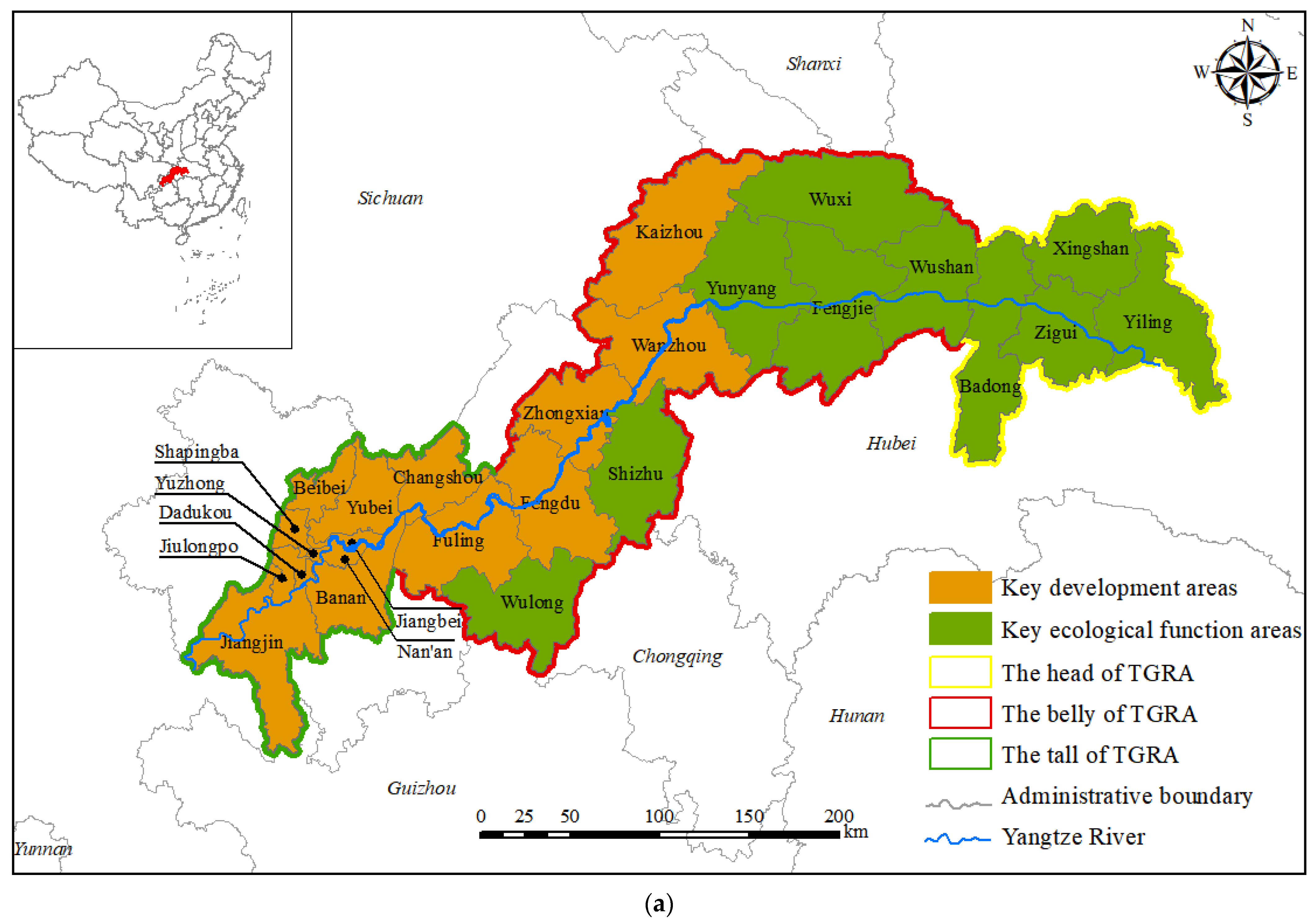
The TGRA refers to the regions affected by inundation due to the construction of the Three Gorges Project of the Yangtze River. It is located at the joining of the Sichuan Basin and the middle and lower reaches of the Yangtze River Plain, from Yiling District in the east to Jiangjin District in the west, covering an area of about 58,000 km2 [42]. Based on the unique characteristics of regional development, the National Main Functional Area Planning positions the TGRA as a key development area and a key ecological functional area. The TGRA consists of three parts: the head, the belly, and the tail of the Reservoir (Figure 1a). The head of the TGRA includes four districts (counties) in Hubei Province: Badong County, Xingshan County, Zigui County, and Yiling District; the belly and tail of the TGRA constitute the Chongqing section of the TGRA, of which, the belly includes Wushan County, Wuxi County, Fengjie County, Yunyang County, Kaizhou District, Wanzhou District, Zhong County, Shizhu County, Fengdu County, Wulong District, and Fuling District; the tail of the Reservoir includes Changshou District, Yubei District, Beibei District, Jiangbei District, Yuzhong District, Nanan District, Shapingba District, Dadukou District, Jiulongpo District, Banan District, and Jiangjin District.
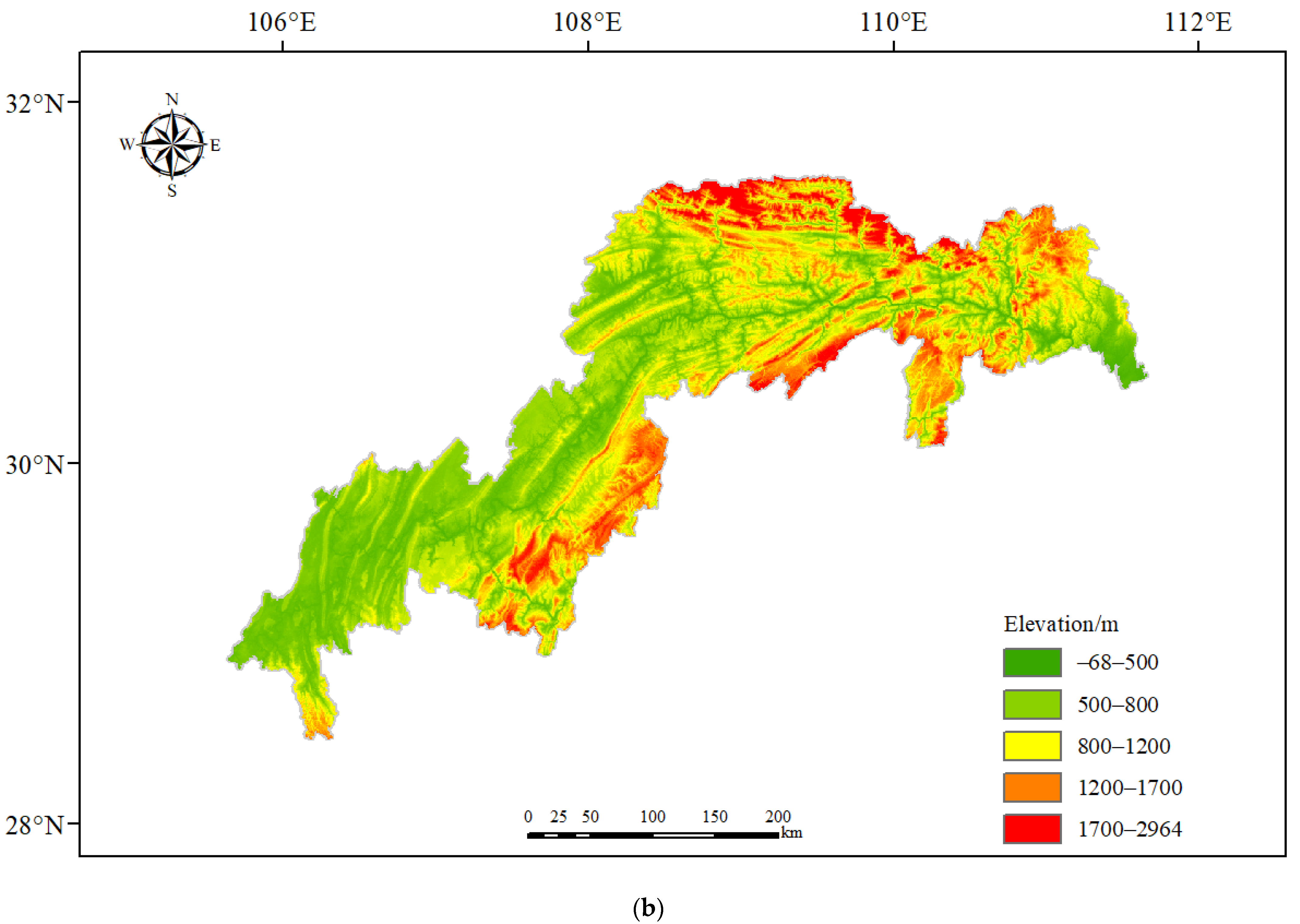
The geographical location of the TGRA is 28°28′ N–31°44′ N, 105°49′ E–111°39′ E. The terrain shows the characteristics of high north and low south, with an elevation between −68 m and 2964 m, numerous mountains, and hilly terrain (Figure 1b). The TGRA has a typical subtropical humid monsoon climate, with an average annual temperature of 15 °C–18 °C, abundant precipitation, average annual precipitation of 1045 mm–1140 mm, more than in the central-eastern part than in other areas, and uneven distribution of surface water resources. Cultivated land and forest land are the primary land-use types in the TGRA. The cultivated and forest land areas accounted for 36.87% and 47.96% of the total area in the TGRA in 2018, respectively. Over the years, the economy of the districts and counties in the TGRA has shown a rapid growth trend. With an average growth rate of 16.86% in the gross national product (GDP) from 2005 to 2018, the resident population increased from 18.73 million in 2005 to 21.03 million in 2018. The region at the tail of the TGRA is mainly the central core city of Chongqing, which has a better economic condition. The region in the middle, from Fuling to Wanzhou, has the latter economic condition. In contrast, the region east of Wanzhou has a mountainous terrain, low productivity, and the worst economic condition.
2.2. Research Methodology
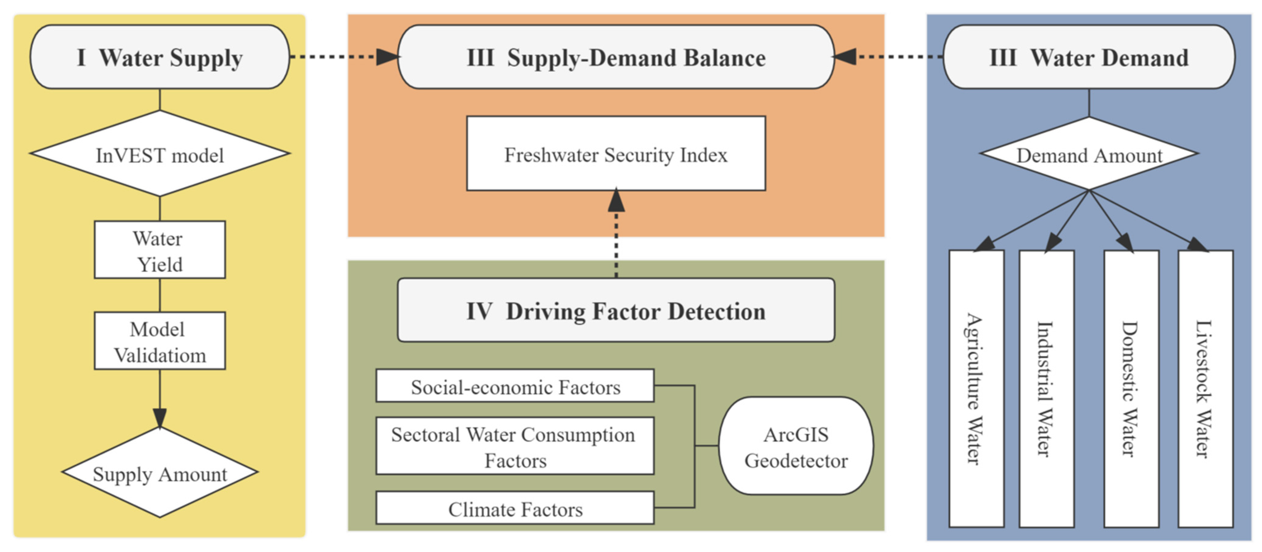
The assessment of the supply and demand of WSSs in the TGRA and the analysis of the driving factors mainly include the following vital steps (Figure 2): (1) Assessing the supply of WSSs by the InVEST annual water yield model, a process that involves adjusting the Z parameter and performing model validation to explore the spatiotemporal variation of water supply in the TGRA (Figure 2I); (2) Constructing WSSs demand model, exploring the spatial and temporal variation of water demand in the TGRA (Figure 2II); (3) Constructing WSSs supply-demand balance model, introducing the FSI and exploring the freshwater security situation in the TGRA (Figure 2III); and (4) Classifying the driving factors, using ArcGIS and Geodetector to investigate the drivers of the FSI under the “natural-social-economic” complex ecosystem (Figure 2IV).
2.2.1. Valuation of Water Supply Services
In this study, the annual water yield (AWY) module of the InVEST model is adopted to calculate the supply of WSSs in the TGRA. The AWY module is based on the water balance principle which does not consider the interaction flow between surface and groundwater. It utilizes the difference between the regional water input precipitation and output evapotranspiration to obtain the regional ecosystem water yield [43]. The specific calculation equation is as follows [33]:
where Yij is the average annual water yield of land use type j on pixel i (mm), Pi is the average annual precipitation on pixel i (mm), AETij is the actual average annual evapotranspiration of land use type j on pixel i (mm), Bij is the Budyko aridity index of land use type j on pixel i (dimensionless), obtained from the evapotranspiration coefficient of land cover type j on pixel i, kij (dimensionless), potential evapotranspiration ET0i (mm), and precipitation Pi. Potential evapotranspiration ET0i is calculated by the Modified-Hargreaves formula, where RA is the solar atmospheric top radiation, Tavg is the mean value of the maximum and minimum temperatures in the TGRA, and TD is the difference between the mean maximum and mean minimum temperatures in the TGRA. The wi is a nonrealistic parameter describing soil properties under natural climatic conditions, obtained from the ratio of the available water content on pixel i, AWCi (mm), to the average annual precipitation, Pi, with the definition of Zhang coefficient Z. MaxSoilDepthi is the maximum soil depth on pixel i (mm). RootDepthi is the root depth on pixel i (mm). PAWC indicates the plant’s available water content (%) and SAN, SIL, CLA, and C represent the soil’s sand, silt, clay, and organic carbon content (%).
2.2.2. Demand for Water Supply Services
This study uses the regional water consumption as a conservative estimate of WSSs demand. According to the definition and classification of water consumption in the ARIES model, the WSSs demand model mainly includes four categories: agricultural water, industrial water, domestic water (including urban domestic and rural domestic water), and livestock water [44]. In the WSSs demand model calculation, this paper refers to the study of Chowdhury [45], selecting the animal virtual water indicator to measure the actual amount of water for livestock. Virtual water is the virtual amount of water quantity condensed in products and services, and as animal products are sold and traded, the water used to produce those products is traded [46]. The virtual water content per unit for the main animal products in the TGRA was extended from the China part of Hoekstra and Chapagain’s research [47] (Table 1). At the same time, physical water indicators were used to measure the consumption of agricultural, industrial, and domestic water. The specific calculation formula is as follows [48]:
where TDx is the total water consumption of the district (county) x (m3), and Dagrx, Dindx, Ddomx, and Dlivx represent agricultural water, industrial water, domestic water, and livestock water of the district (county) x (m3). Aagrx is the area of cultivated land (mu) and Magrx is the average irrigation water consumption per mu of cultivated land (m3/mu) of the district (county) x. AGDPx is the gross industrial production (million yuan) and MGDPx is the water consumption per million yuan of gross industrial production (m3/million yuan) of the district (county) x. Aurx is the number of permanent urban residents and Murx indicates the daily water consumption of urban residents (m3/person) of the district (county) x. Arrx is the number of permanent rural residents and Mrrx indicates the daily water consumption of rural residents (m3/person) of the district (county) x. VWCxi is the unit virtual water content of the livestock product i, Lxi is the production of the livestock product i of the districts (counties) x, and n is the total number of significant livestock products consumed in the region.
2.2.3. Supply-Demand Balance Analysis of Water Supply Services
The freshwater security index (FSI) is calculated by correcting the ratio of supply to demand (Y:D) [49] which is defined as the logarithmic transformation of the ratio of supply to demand of WSSs. The FSI assesses the supply-demand balance of WSSs in the TGRA. When the FSI is more significant than zero, it indicates a surplus of WSSs, and the supply of water resources is higher than the demand. In this case, the district (county) is the WSSs supply region. However, when the FSI is less than zero, it indicates a deficit of WSSs, and the demand for water resources is greater than the supply. In this case, the district (county) is the WSSs beneficiary region [50]. The calculation formula is as follows:
where FSIx denotes the freshwater security index of the district (country) x, Yx denotes the average annual supply of WSSs of the district (country) x and Dx denotes the average annual demand of WSSs in the district (country) x.
2.2.4. Geodetector
This study simulates the supply and demand of WSSs in the TGRA, aiming to improve regional freshwater security and provide scientific support for the government to implement water resource management and ecological compensation policies. Moreover, analyzing the utilization structure of freshwater resources in the TGRA and exploring the main drivers of freshwater security in the TGRA can enable the government to make effective regulations for different regional characteristics [51]. Geodetector is a set of statistical methods to detect spatial heterogeneity and reveal the driving forces behind it. It can detect the spatial heterogeneity of geographical objects and analyze the driving effects between variables by examining the spatial coupling of two variables [52]. The Geodetector factor monitoring is as follows:
where L is the number of classifications of the variables, and X and Y variables are superimposed in the Y direction to form L layers, denoted by h = 1, 2…, L. N and Nh are the sample numbers of the whole region, and subregion h, respectively. and are the discrete variances of the whole region Y and subregion h, respectively. The q denotes the explanatory factor rate, with a value from 0 to 1; the larger the value of q, the stronger the explanatory power, and vice versa.
The spatiotemporal differentiation of freshwater security patterns is subject to the combined effect of various natural and socio-economic factors. Based on the relevant literature [53] and the actual context of the TGRA, this article investigated the magnitude of the influence of a total of 13 socio-economic, sectoral water consumption, and climatic factors on the spatiotemporal variation of FSI in the TGRA by the Geodetector. The specific factors and codes are shown in Table 2. The experimental calculations were conducted in ArcGIS 10.7 (process FSI and various factors) and Geodetector 2015.
2.3. Data
2.3.1. Supply Data
The Digital Elevation Model (DEM) data were obtained from the Geospatial Data Cloud (https://www.gscloud.cn/search, accessed on 25 December 2021) with a spatial resolution of 30 m × 30 m. The precipitation data were obtained from the China Meteorological Data Network (https://data.cma.cn, accessed on 5 January 2022) with a spatial resolution of 1 km × 1 km. Solar radiation data were obtained from the WorldClim (https://www.worldclim.org, accessed on 5 January 2022) and temperature data were obtained from the China Meteorological Data Network (https://data.cma.cn, accessed on 5 January 2022). The root restricting layer depth of soil and the content of sand, silt, clay, and organic carbon were obtained from the 1:1 million soil database of the National Cryosphere Desert Data Center (http://data.casnw.net/portal, accessed on 5 January 2022). Land use data were obtained from the Resource and Environment Data Cloud Platform, Chinese Academy of Sciences (https://www.resdc.cn, accessed on 5 January 2022), with a spatial resolution of 30 m × 30 m. In this study, the land in the TGRA was divided into 6 primary land classes (cultivated land, forest land, grassland, water, construction land, and unused land) and 18 secondary land classes according to the Chinese Academy of Sciences. The evapotranspiration coefficients and maximum root depth of each land class were obtained by referring to the research by Yang et al. [54]. Finally, the biophysical table for running the InVEST annual water yield model is shown in Table 3.
2.3.2. Demand Data
The multi-year gross industrial production, resident population, and livestock product output of socio-economic category data of each district (country) in the TGRA were obtained from The Economic and Social Characteristics Development Database of the Three Gorges Reservoir Area (https://sanxia.ctbu.edu.cn/index.htm, accessed on 25 December 2021). The multi-year cultivated land area of each district (country) in the TGRA was obtained from land-use data extracted and analyzed in ArcGIS 10.7. Unit water consumption indicators were obtained from the Water Resources Bureau of each local city.
3. Results and Analysis
3.1. Validation and Processing of Model Parameter
Model validation refers to comparing the results of model runs with measured data to determine the most suitable assessment model for the study area by adjusting the seasonality factor [24]. The Zhang coefficient is a seasonal parameter that reflects the seasonal distribution characteristics of precipitation and hydrogeological features, and its range is generally 0–30. For areas with equal total precipitation, the more frequent the precipitation is, the larger the parameter Z is. The monitoring data from hydrological stations are cross-sectional runoff data, which cannot accurately reflect the natural runoff in the region [55]. Therefore, it is not easy to directly use the runoff data from hydrological stations to verify the results of the InVEST model. In this study, surface water resources were selected for evaluating the actual and simulated results. Due to the limitation of surface water resource data in the TGRA (Hubei section), the article adopts the annual average surface water resources in the TGRA (Chongqing section) as the basis for determining the Z parameter. The data were obtained from the Chongqing Water Resources Bulletin (2005–2018). For model validation, three indicators, correlation coefficient R2, root mean square error (RMSE), and the Nash–Sutcliffe efficiency coefficient (NSE), were used to evaluate the simulation effects of the InVEST model. The equations are as follows [56]:
Qstai and represent the average annual surface water resources of the district (county) i and the TGRA (Chongqing section), respectively, as reported in the Water Resources Bulletin. n represents the number of administrative units and R2 is used to evaluate the fit between the statistical and simulated values, ranging from 0 to 1. The closer R2 is to 1, the better the simulation, and vice versa. RMSE reflects the deviation between the simulated and statistical values. NSE is an essential indicator for evaluating the quality of a model and is usually used to evaluate the accuracy of hydrological model simulations with a value between 0 and 1. The closer the value is to 1, the better the model simulation is, meaning that the model simulation value is closer to the statistical value and vice versa. It is generally accepted that simulation accuracy is desirable with R2 > 0.60 and NSE > 0.50 [57].
After repeatedly adjusting the seasonal parameter values, when Z = 6.39, the simulated values were verified against the statistical values to obtain R2 = 0.69, Prob < 0.01, n = 22, RMSE = 6.44 × 10⁸ m3, and NSE = 0.64, indicating that the InVEST annual water yield model applies to the TGRA research.
3.2. Spatiotemporal Variation in the Supply of Water Supply Services
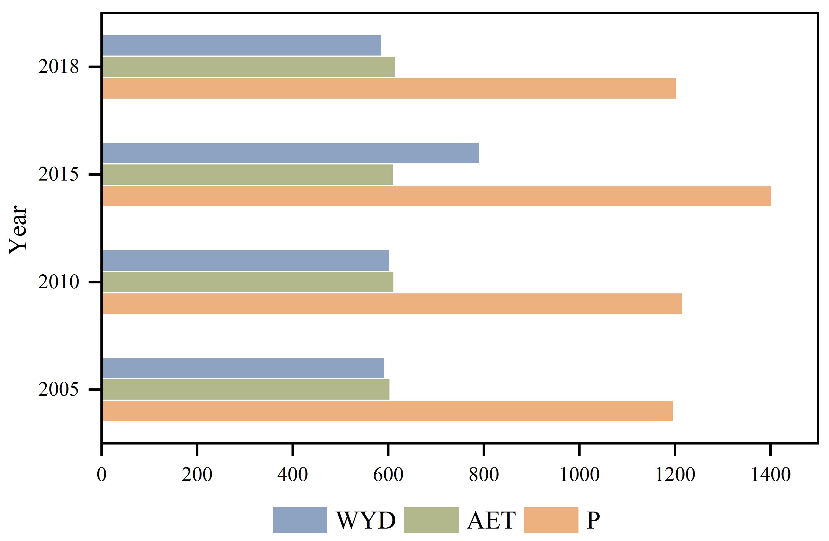
On the time scale, the annual water yield in the TGRA showed a trend of first increasing and then decreasing from 2000 to 2018. Compared with 2005, the water yield depth increased by 10.19 mm (water yield increased by 0.23 × 10⁸ m3) in 2010, 197.43 mm (water yield increased by 4.43 × 10⁸ m3) in 2015, and 6.36 mm (water yield decreased by 0.14 × 10⁸ m3) in 2018. From 2005 to 2018, the overall decrease in water yield depth was 1.07%, and the overall decrease in water yield was 1.05%. Additionally, from 2005 to 2018, the overall increase in precipitation and actual evapotranspiration in the TGRA was 0.56% and 2.05%. The precipitation reached a maximum of 1402.79 mm in 2015, and the actual evapotranspiration reached a maximum of 616.09 mm in 2018. The 2005 precipitation and actual evapotranspiration were the smallest, 1196.85 mm and 603.69 mm, respectively (Figure 3); influenced by multiple factors such as precipitation and evapotranspiration, the highest water yield was in 2015 and the lowest in 2018 in the TGRA.
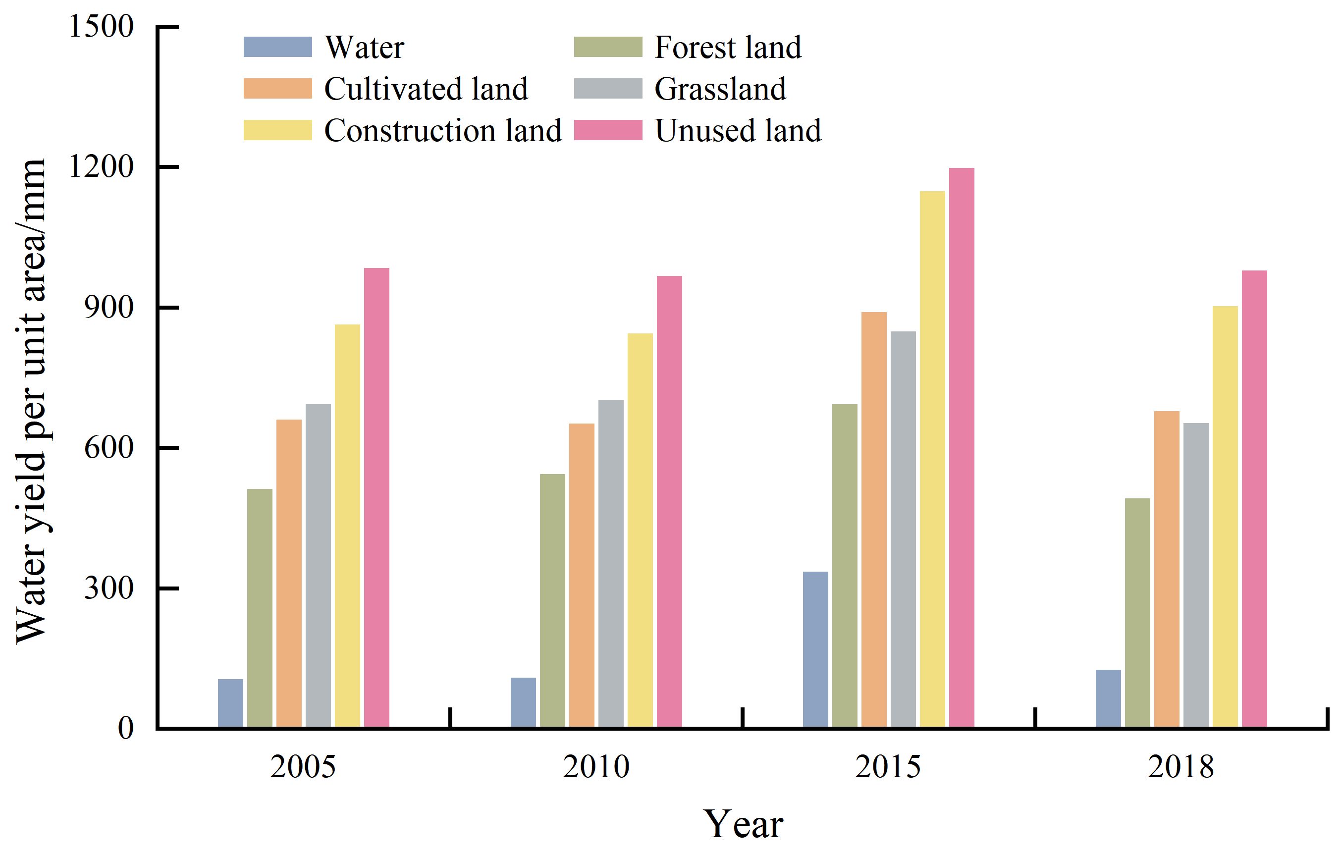
Regarding land use types, the most significant average water output from 2005 to 2018 was cultivated land (156.29 × 10⁸ m3), accounting for 42.36% of the multi-year average water yield in the TGRA. The minuscule average water output was unused land (5.2 × 10⁶ m3), accounting for only 0.01% of the multi-year average water yield in the TGRA. The water yield per unit area of all types of land showed a rising and then declining trend from 2005 to 2018 (Figure 4). The water yield per unit area of all types of land ranks from high to low as unused land > construction land > grassland > cultivated land > forest land > water.
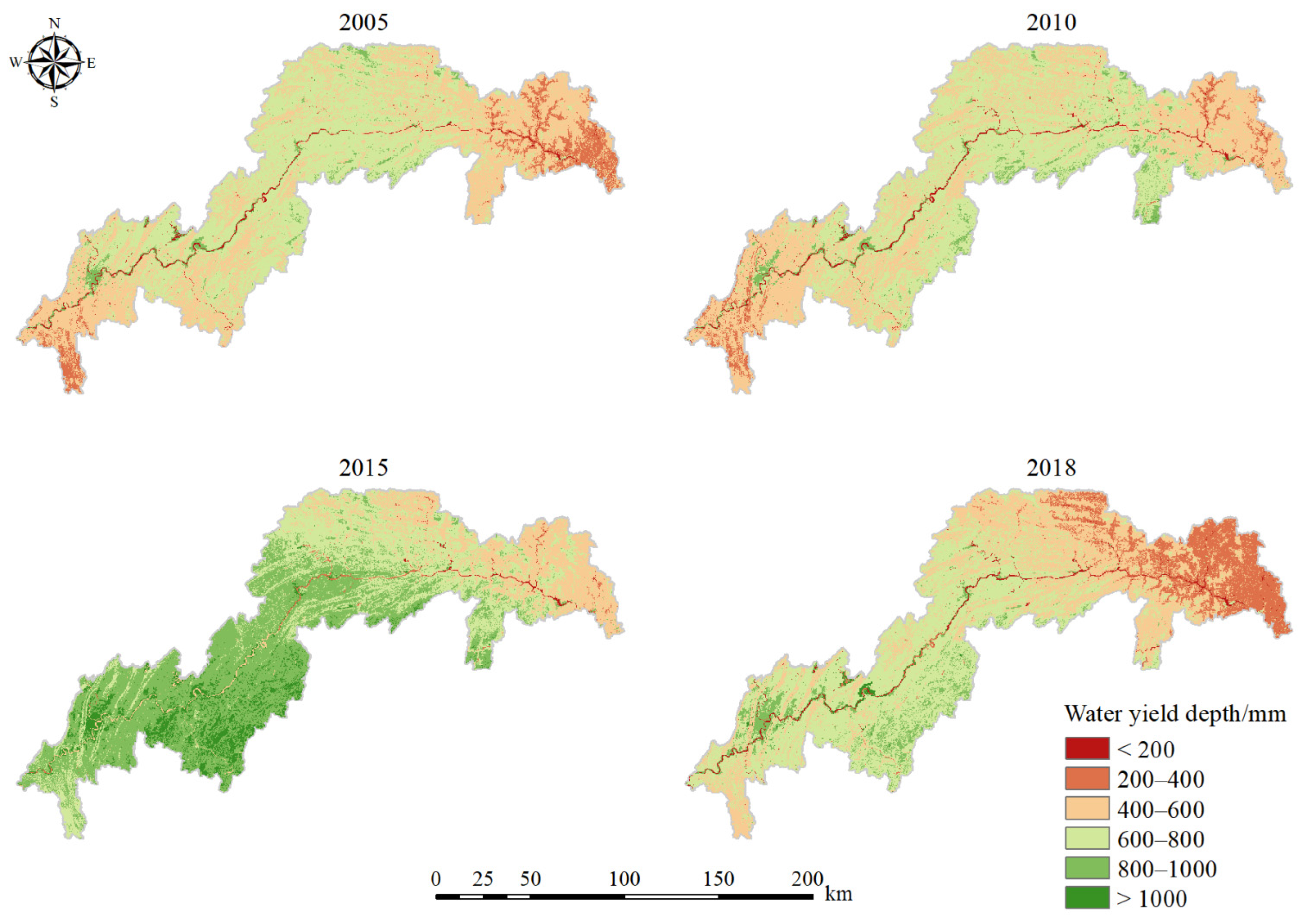
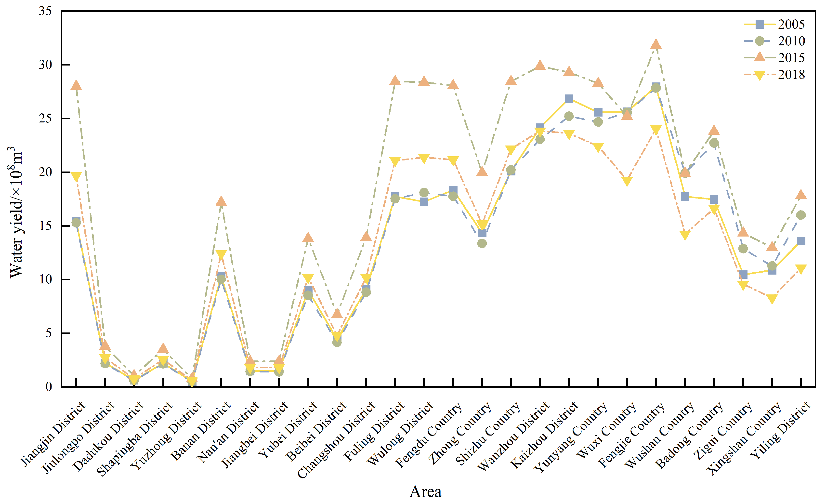
On the spatial scale, the spatial distribution of water yield depth in the TGRA from 2005 to 2018 did not vary greatly and showed a consistent distribution across years, with lower water yield depth in the head and tail of the TGRA and higher water yield depth in the belly (Figure 5). The high-value water yield areas from 2005 to 2018 were concentrated in Fengjie County, Kaizhou District, Yunyang County, Wanzhou District, Wuxi County, and Shizhu County in the belly of the TGRA, with the multi-year average water yield in the range of 22.75 × 10⁸ m3–27.93 × 10⁸ m3. The low-value areas are concentrated in Jiulongpo, Shapingba, Nanan, Jiangbei, Dadukou, and Yuzhong districts in the tail of the TGRA, with the multi-year average water yield fluctuating between 0.59 × 10⁸ m3 and 2.73 × 10⁸ m3 (Figure 6). In total, 15 districts and counties increased in water yield, though the overall water yield in the TGRA decreased by 1.05%. In addition to the precipitation, actual evapotranspiration, and land use type, the administrative area’s size also affects the WSS supply of WSSs. For example, Fengjie County has a lower average multi-year precipitation than Shizhu County. However, its annual supply of WSSs is the highest because Fengjie County has the largest catchment area and, therefore, high water yield, as its total area is at the top of the 26 districts (countries) in the TGRA (4177.59 km2).
In addition, from the perspective of water yield per unit area in each district and county, the precipitation in 2005 and 2010 in Xingshan County was greater than that in Yuzhong District. However, the water yield per unit area in Yuzhong District was much higher than that in Xingshan County. Most of the land in Yuzhong District is construction land, accounting for 81.14% of the area of Yuzhong District, while the proportion of forest land is only 0.94%. The land type of Xingshan County is mainly forest land, which accounts for 88.74% of the area of Xingshan County, while the proportion of construction land is only 0.18%, much lower than that of the Yuzhong District. To a certain extent, this also proves that the water yield capacity of construction land is higher than that of vegetation-covered areas such as forest land. However, urbanization construction increases the surface hardening rate; the impervious area increases, and the water yield and sink characteristics change. After regional rainfall, the decrease in soil infiltration causes a large amount of rainwater to remain on the surface, increasing surface runoff from precipitation, thus significantly reducing the number of ways that rainfall infiltrates to recharge groundwater, resulting in insufficient groundwater recharge and making it difficult for water resources to be used [58]. In addition, rainfall falling on the impermeable ground has fast water flow and short confluence time. In the case of heavy precipitation, flood peaks can easily form and cause severe urban flooding, which greatly tests the urban flood control and flood drainage system.
3.3. Spatiotemporal Variation in the Demand for Water Supply Services
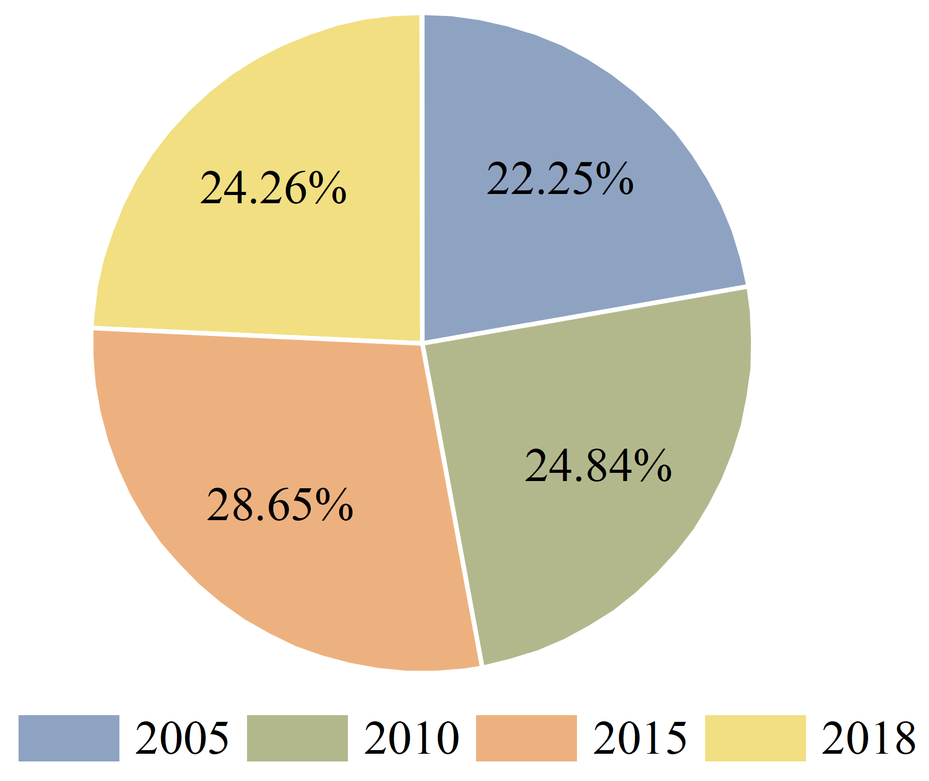
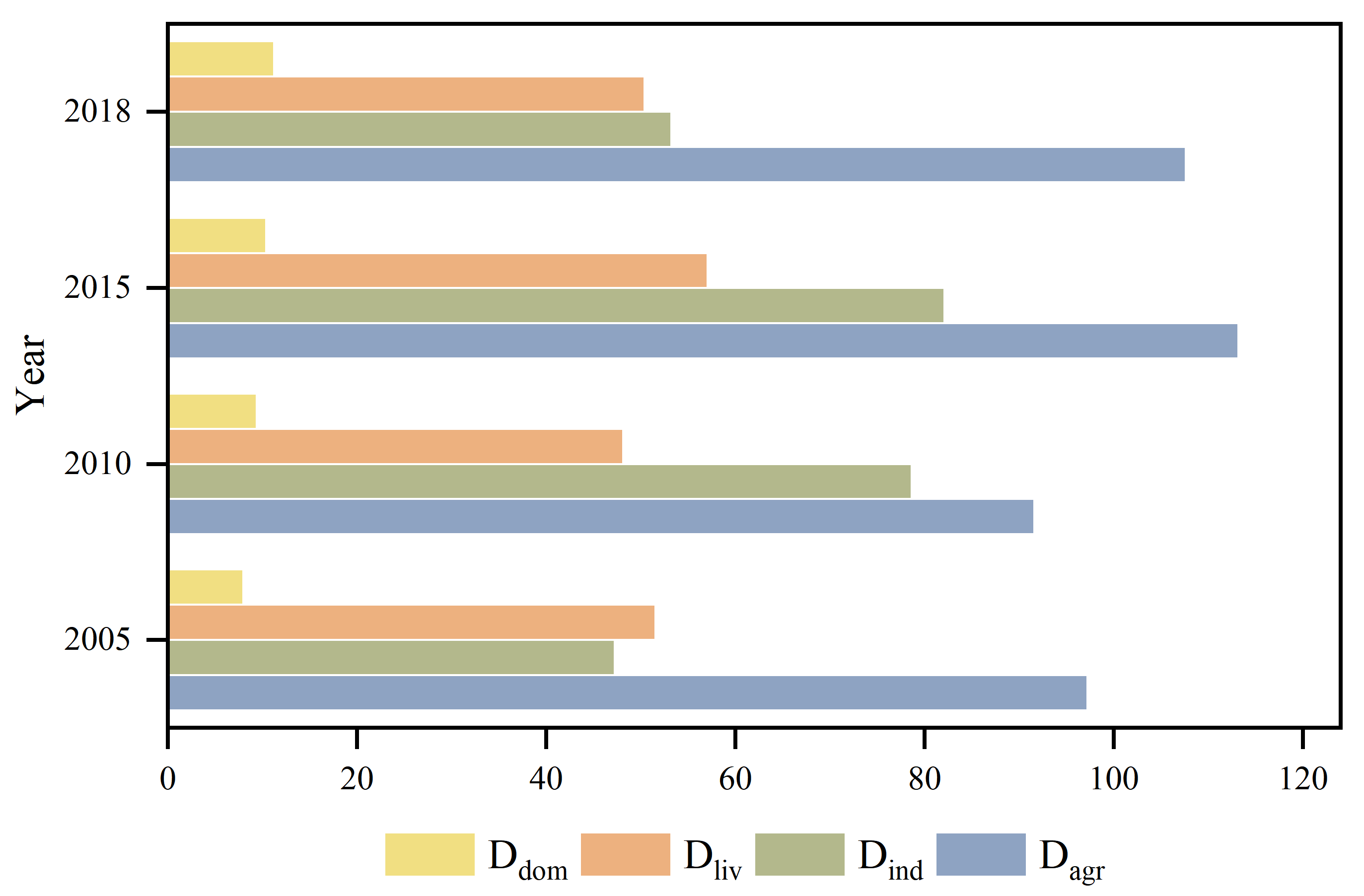
On the time scale, in terms of the total water consumption, the total water consumption in the TGRA from 2005 to 2018 showed a trend of first rising and then declining. The highest total water consumption was in 2015 (262.76 × 10⁸ m3), accounting for 28.65% of the total multi-year water consumption in the TGRA. The lowest total water consumption in 2005 (204 × 108 m3) accounted for 22.25% of the total multi-year water consumption in the TGRA (Figure 7). Overall, the total water consumption in the TGRA increased, with total water consumption increasing by 9.1% (18.46 × 10⁸ m3) in 2018 compared to 2005. In terms of water consumption by sector, the trend of water consumption by sector in the TGRA from 2005 to 2018 was different, with the agricultural water consumption showing a trend of first decreasing and then increasing. The multi-year water consumption in agriculture was 97.22 × 10⁸ m3, 91.6 × 10⁸ m3, 113.17 × 10⁸ m3, and 107.63 × 10⁸ m3, respectively. Industrial water consumption showed a trend of first increasing and then decreasing and was 47.25 × 10⁸ m3, 78.65 × 10⁸ m3, 82.11 × 10⁸ m3, and 53.21 × 10⁸ m3. The livestock water consumption showed a decreasing trend, with livestock water consumption over the studied years being 51.57 × 10⁸ m3, 48.15 × 10⁸ m3, 57.09 × 10⁸ m3, and 50.4 × 10⁸ m3. Domestic Water consumption shows a rising trend year by year, with residents consuming 7.97 × 10⁸ m3, 9.4 × 10⁸ m3, 10.39 × 10⁸ m3, and 11.23 × 10⁸ m3, respectively (Figure 8).
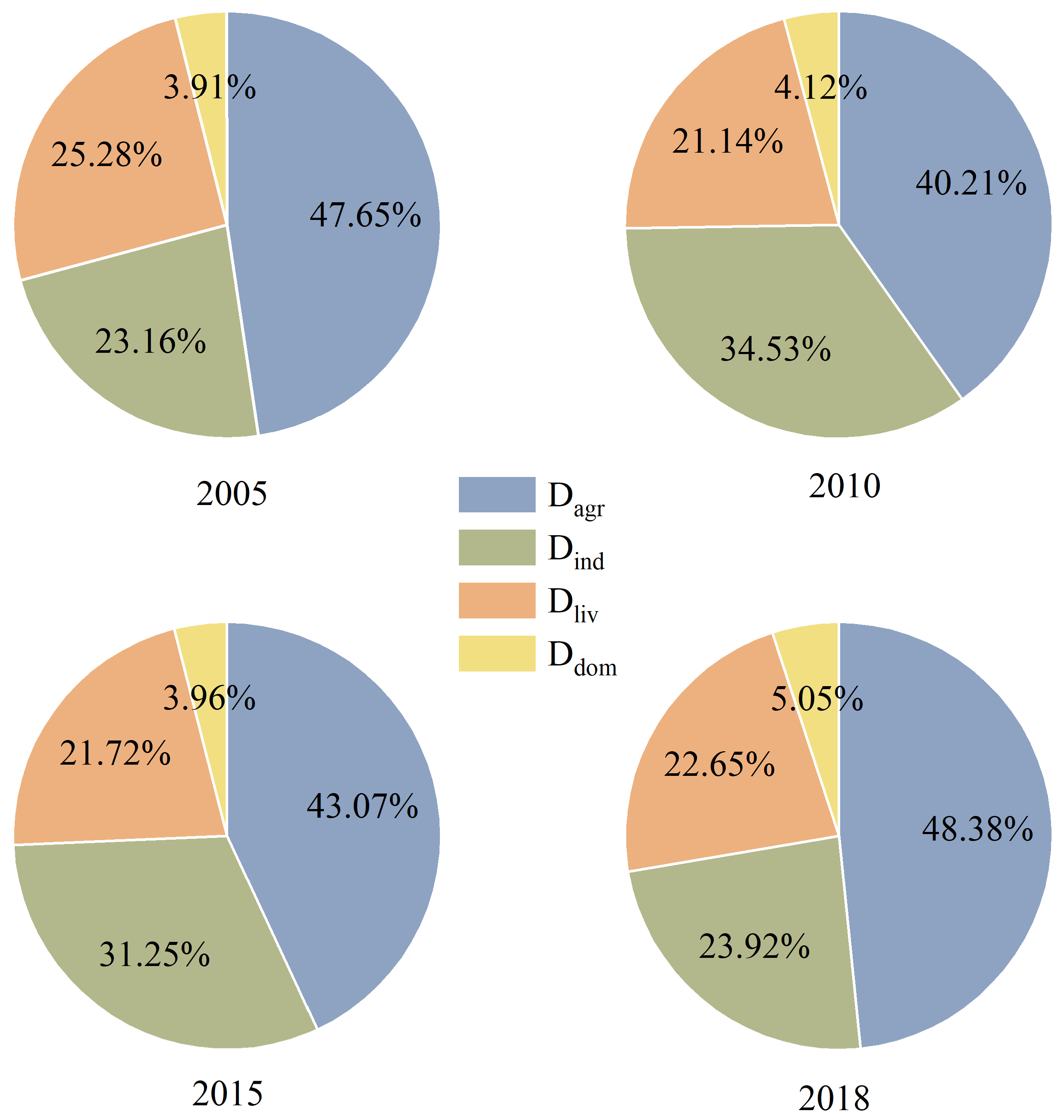
Agricultural water is the main water used in the TGRA, accounting for 44.67% of the total multi-year water consumption. Compared with 2005, the proportion of agricultural water in the TGRA increased by 0.73%, industrial water increased by 0.76%, livestock water decreased by 2.63%, and domestic water increased by 1.14% in 2018 (Figure 9). The proportion of domestic water consumption increased the most, reflecting the rapid growth of the population in the TGRA, which led to the increased demand for water in residents’ daily life. The decrease in the proportion of livestock water is mainly due to the reduction in pork and milk production in the TGRA, which dropped by 16.9% and 53.66% in 2018 compared with 2005.
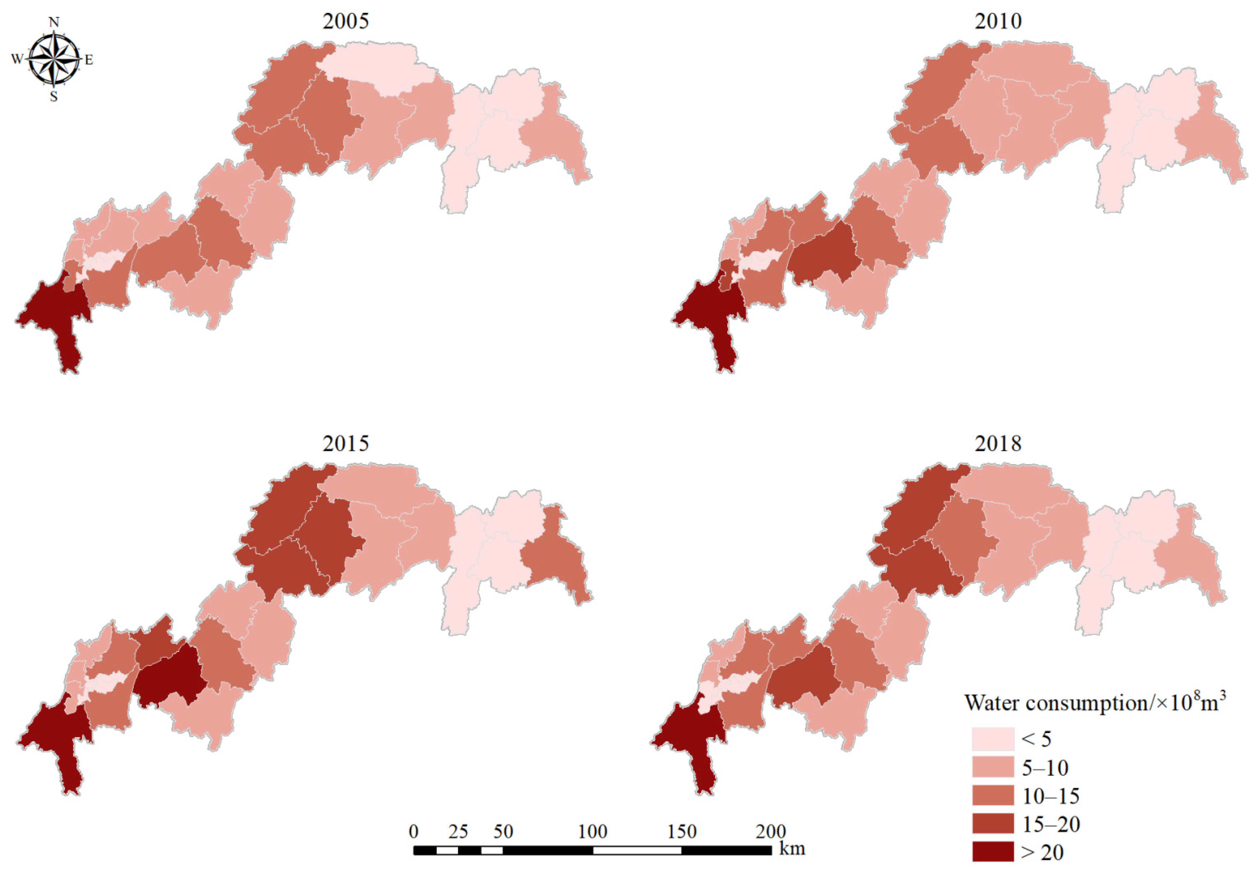
On the spatial scale, the water consumption in the tail and the middle of the belly of the TGRA was relatively high from 2005 to 2018. In comparison, the water consumption in the head of the TGRA was low (Figure 10). The variation in water consumption in each district and county from 2005 to 2018 is shown in Figure 11. The high water consumption areas are mainly concentrated in Jiangjin, Fuling, Kaizhou, Wanzhou, Changshou, and Banan districts, with the average water consumption fluctuating within the range of 12.53 × 10⁸ m3 to 24.57 × 10⁸ m3 over the studied years. These districts are located in the key development zones of the TGRA. They are also concentrated areas of industry, agriculture, and breeding, having a large population and significant water demand in various sectors. The low-value water consumption areas are mainly Badong County, Zigui County, and Xingshan County at the head of the TGRA and Yuzhong District, Jiangbei District, and Dadukou District at the tail of the TGRA, with the average multi-year water consumption concentrated at 0.62 × 10⁸ m3–3.72 × 10⁸ m3. Among them, the land types of Zigui County, Badong County, and Xingshan County are mainly forest land with a comparatively low residential population. At the same time, Yuzhong District, Jiangbei District, and Dadukou District are the main urban areas of Chongqing, focusing on the development of the financial service industry. Moreover, the regional development pattern has a low demand for agricultural and livestock water, thus being a low-value area for water consumption.
In terms of water consumption by sector, from 2005 to 2018, the highest water consumption for agriculture and livestock was in Kaizhou District, with cumulative multi-year agricultural water consumption reaching 40.75 × 10⁸ m3 and cumulative multi-year livestock water consumption reaching 16.43 × 10⁸ m3. The highest water consumption for the industry was in the Jiangjin District, with cumulative multi-year industrial water consumption reaching 56.39 × 10⁸ m3; the highest domestic water consumption was in Jiulongpo District, with cumulative water consumption of 3.15 × 10⁸ m3 over the years.
3.4. Spatiotemporal Variation in the FSI of Water Supply Services
Based on the FSI and ArcGIS 10.7, the spatial and temporal distribution pattern of the supply and demand balance of WSSs in the TGRA was obtained (Figure 12). In order to more intuitively reflect the contradictory situation of regional water supply and demand, as well as the spatiotemporal variation characteristics, the FSI was divided into four categories: <−0.5, −0.5–0, 0–0.5, and >0.5.
On the time scale, the overall supply of WSSs in the TGRA was more significant than the demand from 2005 to 2018, and the average annual FSI was 0.12, 0.10, 0.21, and 0.16, showing an upward trend in general. The number of districts and counties with a shortage of WSSs are 10, 12, 9, and 9, indicating a decreasing and stabilizing trend. As discussed by period, from 2005 to 2010 and from 2015 to 2018, the FSI decreased due to the rapid progress of society and the rapid growth of the population, human demand increased, and water consumption of all kinds increased, making the supply and demand of WSSs balanced to reach a lower value. From 2005 to 2010, the FSI of WSSs reached a maximum value after balancing supply and demand, mainly because 2015 was a year of abundant water, with a significant increase in annual precipitation and a more prosperous supply of water resources. From 2005 to 2018, the economy and society were developing rapidly. However, the FSI in the TGRA increased, mainly in response to the national policy and the construction of a water-saving society; Hubei Province and Chongqing Municipality included water conservation in their social development programs and issued the Water Consumption Quotas for Industries in Hubei Province (2017) and Chongqing Municipality Water Conservation Management Measures (2018). As a result, water consumption in the TGRA has been effectively supervised, contributing to the improvement of FSI.
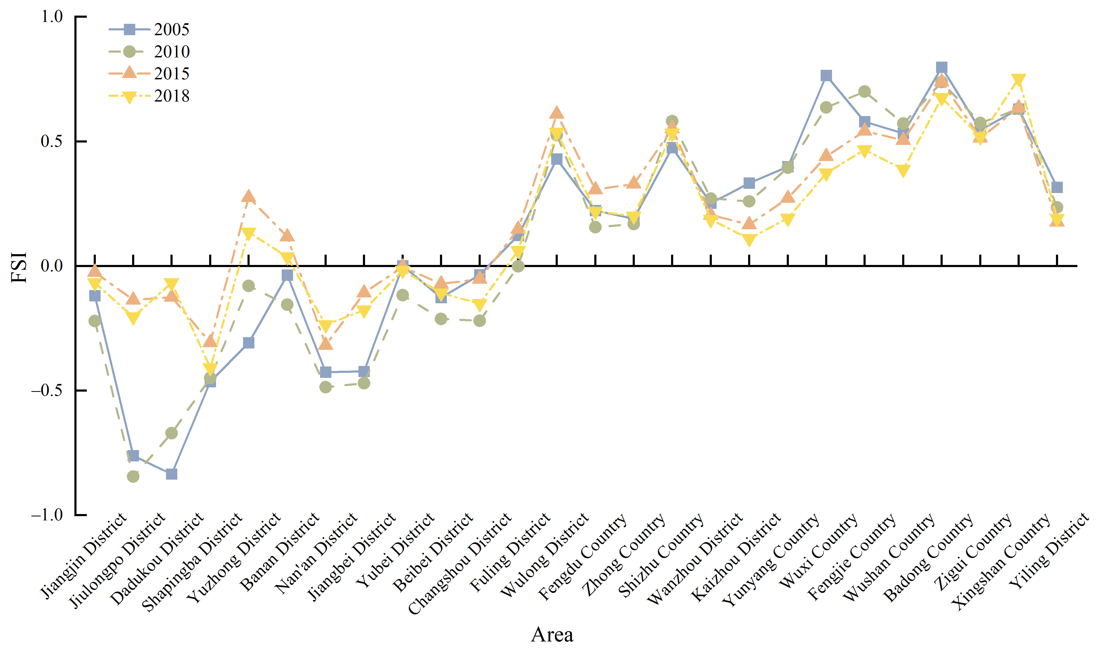
On the spatial scale, the multi-year average FSI of each district and county in the TGRA fluctuates between −0.49 and 0.74 (Figure 13). The high FSI zones are mainly concentrated in the key ecological function areas. In contrast, the low FSI areas are mainly located in the Reservoir tail zones in the key development areas. From 2005 to 2018, Beibei, Jiangbei, Nanan, Shapingba, Dadukou, and Jiulongpo districts have a shortage of WSSs, with their multi-year average FSI ranging from −0.49 to 0.13. The primary reason for the low FSI is that the districts mentioned above are low-value water yield regions, accounting for only 3.9% of the total annual water yield of the entire TGRA, with a limited urban water supply capacity. At the same time, the districts mentioned above are located in the core urban region of Chongqing, with rapid economic development and urbanization, and construction land accounts for 32.21% of the entire TGRA. For many years, the total gross industrial production and urban domestic water consumption reached 39.94% and 41.67% of the entire TGRA; thus, the demand for WSSs is high.
However, most of the remaining districts and counties have surplus water resources, especially in Shizhu, Wuxi, and Fengjie counties at the belly of the TGRA and Badong, Xingshan, and Zigui counties at the head of the TGRA where the multi-year average FSI ranges from 0.54 to 0.74. On the one hand, the counties mentioned above have relatively sufficient water yield, especially in Shizhu, Wuxi, and Fengjie counties. The total multi-year supply of the WSSs reaches 19.91% of the whole TGRA. On the other hand, the land-use types of these counties with higher FSI are mainly forest land, and the multi-year average forest land areas reached 44.52% of the forest land areas of the entire TGRA. In contrast, the construction land areas are relatively minor, accounting for only 7.3% of that in the TGRA; so, the residential population is small, the water demand is moderate, and consequently, the demand for WSSs is scarce. In general, each year, the surplus and shortage of WSSs in the TGRA follow the national functional positioning of its different regions.
3.5. Geodetector Analysis
This article measured the magnitude of the influence of 13 factors on FSI in the TGRA by Geodetector (Table 4). The results show that socio-economically, freshwater security in the TGRA is mainly influenced by gross industrial production and the resident population, where the impact of gross industrial production is relatively stable from year to year, while the influence of population-level increases year by year. Gross industrial production had the most significant effect on the spatial variation of freshwater security in 2005. Nevertheless, in 2010, aquatic production was the critical driver of freshwater security in the TGRA, reflecting the heavy impact of fisheries on the water environment in that year. From 2010 to 2018, the dominant factor of FSI is the resident population, revealing that the rapidly growing population has progressively higher effects on freshwater security in the TGRA. As for water consumption in all sectors, FSI in the TGRA is mainly driven by industrial and domestic water consumption, enhancing the influence of both. Regarding the natural climate, precipitation is the leading driver of FSI in the TGRA; the overall increase in q-value indicates that freshwater security in the TGRA is dependent on it the most.
From 2005 to 2018, among all drivers, industrial water consumption has the most positive contribution and an increasing trend. The q value of industrial water consumption in 2018 increased by 43.55% compared with 2005, indicating that the leading factor of freshwater security in the TGRA is industrial water consumption, and its influence is gradually increasing. While the rise in q value of industrial water consumption compared to gross industrial production is considerable, reflecting the increasing consumption of unit water resources by industrial technology production methods in the TGRA with the development of high-quality industrial industries. Nevertheless, the contribution of cultivated land area to agricultural water consumption from 2005 to 2018 shows a decreasing trend. However, the q-value of agricultural water consumption compared to cultivated land area decreases to a greater extent, showing the improvement of agricultural irrigation methods and technology in the TGRA and the enhancement of agricultural water utilization efficiency. Meanwhile, the influence of domestic water consumption on FSI in the TGRA increased significantly with the rapid population growth in recent years. In contrast, the influence of livestock water consumption varies and eventually reaches stability with the change in the output of all livestock products.
Overall, industrial water consumption has the strongest explanatory power for FSI in the TGRA, and actual evapotranspiration has the weakest explanatory power for FSI. The explanatory rate of industrial and domestic water consumption on FSI keeps growing among the different water consumption sectors while the explanatory rate of livestock water consumption on FSI tends to stabilize, and the explanatory rate of agricultural water consumption on FSI reduces.
4. Discussion
The TGRA is the economic, shipping, and trade logistics center for the “Yangtze River Protection” in China, as well as an essential strategic pivot point for the “Western Development” policy and a critical linkage point for the “Belt and Road” initiative and the Yangtze River Economic Belt strategy [59]. Due to the spatial heterogeneity of the geographical environment and resource base in the TGRA, the socio-economic development also shows distinct unevenness, which are the primary reasons for the imbalance of freshwater resources in the TGRA [60]. The selection of the TGRA as the study area for the supply and demand assessment of WSSs and the detection of driving factors is not only conducive to promoting the sustainable economic and social development of the TGRA, but also to maintaining the Yangtze River economic belt and the Yangtze River basin water resource security strategic management and socio-economic quality improvement as well as contributing to the construction of the ecological basin civilization.
As an essential node linking the upper reaches of the Yangtze River with the middle and lower reaches, the unique geographical location of the TGRA has given it special responsibilities and missions. With the integrated use of InVEST model, ArcGIS, and Geodetector, compared with other related studies, the WSSs in the TGRA showed apparent regional characteristics. First, the water supply is generally higher in the upper part of the basin, which is the main supply area for WSSs, while the lower part is usually the beneficiary area for WSSs [61]. In this study, the tail of the TGRA is located upstream of the head of the TGRA. However, it was found that most of the districts and counties located in the upper part of the watershed had FSI values less than 0 and were the beneficiary areas of WSSs. In contrast, the districts and counties located downstream of the WSSs had more surpluses, and FSI values were more significant than 0 for the supply areas of WSSs. This indicates that the surplus and shortage of WSSs depend on not only the natural geographic conditions but that a large part of it is related to the region’s economic development pattern and condition. Meanwhile, compared with other regions, such as the Lianshui basin [62] and Shiyang River basin [61], the absolute values of FSI in all districts and counties in the TGRA from 2005 to 2018 were less than 1. The average value of multi-year FSI was close to 0, indicating that the administrative units in the TGRA are relatively balanced in terms of supply and demand for WSSs and match the abundant watershed resources and rapidly developing eco-society in the TGRA. Finally, in detecting the driving factors, this study found that industrial production methods and agricultural irrigation techniques affect the water security status and efficiency improvement contributes to reducing water consumption, consistent with Li et al. [63]. In addition, the number of permanent population increases made the q value of domestic water consumption rise the most. Therefore, the institution structure needs to focus on the holistic and systematic arrangement of regulatory tools to properly utilize the strategic reserve of freshwater resources in the TGRA.
In the light of the above research, this article proposes the following targeted policy recommendations. Firstly, based on the limitation and usefulness of water resources, the design of a strategic reserve system for freshwater resources in the TGRA should introduce the two central concepts of adequate protection and rational utilization [64]. As an essential part of the Yangtze River, the TGRA should strengthen the functional role of the freshwater resource reserve under the guarantee of the Yangtze River Protection Law and explore systematic institutional arrangements through departmental regulations and regional synergy legislation and policy formulation [65]. Furthermore, there should be regular interaction between the water environment management departments upstream and downstream of the TGRA [66]. Secondly, the horizontal ecological compensation system should be improved for freshwater resources. The freshwater resource beneficiary administrative region of the TGRA should compensate the ecological protection zone. Moreover, the construction of a diversified and market-oriented ecological compensation mechanism should be explored upstream and downstream of the TGRA, which is a combination of government guidance and market operation, to ensure the sustainable and coordinated development of the “ecology-production-living” space [67]. Thirdly, industrial water conservation technology should be upgraded since industrial water consumption is a crucial factor affecting freshwater security in the TGRA. In the face of rapid economic development and growing industrial water demand, it is essential to set industrial water quotas, investigate new approaches to industrial water saving, and introduce new technologies to reduce industrial pollution and boost water efficiency [68]. Finally, there is a need to raise the residents’ awareness of water conservation and environmental concerns, increase the publicity of water-saving and water consumption policies, and popularize knowledge of water resources and the environment. Simultaneously, the water consumption quota should be controlled and water charges adjusted reasonably to effectively regulate and guarantee domestic water consumption in the TGRA [69].
This paper explores a research framework for assessing the supply and demand of WSSs in the TGRA and analyzing the driving factors, exploring spatial and temporal heterogeneity of WSSs in the TGRA at the county scale. At the same time, the functional positioning of each region in the TGRA is integrated with WSSs. The detection of the driving factors is combined to formulate locally appropriate countermeasures and recommendations which can help promote the management of freshwater security in the TGRA. This study can provide a foundation for regional water resource allocation and ecological compensation policy formulation, as well as provide a reference for other large reservoirs or specific reservoir areas. However, this study also has some limitations. Due to the uncertainty of natural ecosystems, model structure and methodology, and input parameters, there are uncertainties when assessing service functions by the InVEST model. Additionally, the research quantifies the WSSs but not the services that are also important to the TGRA, such as carbon sequestration, oxygen release, and water containment. In addition, it focuses on the spatiotemporal variation of the supply-demand balance of WSSs but does not consider the flow direction, flow path, and flow rate of WSSs. A future study should perform sensitivity analysis on the model’s main parameters to improve the model evaluation’s accuracy. Simultaneously, the diversity of ecosystem services in the TGRA should be considered as comprehensively as possible and strengthen the study of ecosystem service flows to provide a more practical scientific basis for ecological environment management and the specific delineation of ecological compensation standards.
5. Conclusions
The construction of a strategic reserve of freshwater resources in the TGRA is a vital element in strengthening the building of an ecological civilization and an essential part of implementing the overall national security concept. Currently, no research has been conducted on the water quantity in the TGRA from the perspective of ecosystem services. This article combines ecosystem services and socio-economics, starting from the “natural-social-economic” angle. Firstly, based on the supply and demand model of WSSs in the TGRA, the spatial and temporal variation of WSSs during 2005–2018 is assessed. Secondly, by combining remote sensing data with economic and social data, the overall and sub-administrative freshwater security of the TGRA over the years is evaluated. Finally, the Geodetector was applied to investigate the various driving factors of the FSI in the TGRA, laying the foundation for ensuring freshwater security and refining the management of freshwater resources. The main conclusions are as follows:
(1) From 2005 to 2018, the supply of WSSs in the TGRA showed a rising trend and then fell. Compared with 2005, it decreased by 0.14 × 10⁸ m3 in 2018. The head and tail zones of the TGRA are low-value areas for water yield, while the high water yield regions are located in the belly of the TGRA. Cultivated land is the land-use type with the highest average multi-year water yield in the TGRA. In terms of water yield capacity per unit area of land, the ability of vegetation-covered lands such as cultivated land, forest land, and grassland is weak, while construction land is significant. Therefore, cities need to strengthen the construction of flood prevention and drainage systems to avoid urban flooding caused by surface hardening.
(2) From 2005 to 2018, the demand for WSSs in the TGRA showed a trend of first rising and then falling, with the total water consumption in 2018 increasing by 18.46 × 10⁸ m3 compared with 2005. The water consumption level is related to each region’s economic development pattern. The water consumption in the tail and central parts of the belly areas is relatively high, while the water consumption in the head of the TGRA is low. Regarding water consumption in each sector, agricultural water is the primary water consumed in the TGRA, accounting for 44.67% of the total multi-year water consumption. At the same time, the rapid growth of the resident population of the TGRA leads to the most significant increase in the proportion of domestic water consumption.
(3) From 2005 to 2018, the overall water resources in the TRGA were in a state of supply exceeding demand. The FSI showed an upward trend, with the number of districts and counties with water shortages gradually decreasing and stabilizing. In the meantime, the programming of social water conservation policies also facilitates freshwater security management. The FSI values of the key ecological function areas in the TGRA are high. In comparison, the FSI values of the Reservoir tail areas in the key development zones are low, reflecting that the surplus and deficit of WSSs in the TGRA are in line with the national functional positioning of its different regions.
(4) The analysis of the Geodetector results shows that industrial water consumption has the most significant explanatory power for FSI in the TGRA and actual evapotranspiration has the weakest explanatory power for FSI. Among the different water consumption sectors, the impact of industrial and domestic water consumption on FSI keeps increasing. In contrast, the influence of agricultural water consumption on FSI decreased, and the livestock water consumption on FSI finally stabilized. The analysis also shows how technological production affects water consumption efficiency, creating the drivers that contribute to the change in FSI.
Author Contributions
Conceptualization, J.H. and Y.Z.; methodology, J.H. and Y.Z.; data curation, Y.Z.; formal analysis, J.H. and Y.Z.; investigation, J.H. and Y.Z.; validation, Y.Z.; visualization, Y.Z.; funding acquisition, J.H.; project administration, J.H. and C.W.; supervision, J.H. and C.W.; resources, J.H. and Y.Z.; writing—original draft, Y.Z.; writing—review and editing, J.H., Y.Z. and C.W. All authors have read and agreed to the published version of the manuscript.
Funding
This research was funded by the Program of the National Social Science Fund of China (The Funder: National Office for Philosophy and Social Sciences, Grant/Award Recipient: Jia He, Grant/Award Number: 18CJY005).
Institutional Review Board Statement
Not applicable.
Informed Consent Statement
Not applicable.
Data Availability Statement
Not applicable.
Acknowledgments
This research was supported by the Upper Yangtze Basin Complex Ecosystem Management Innovation Team.
Conflicts of Interest
The authors declare no conflict of interest.
References
- Costanza, R.; D’Arge, R.; Groot, R.D.; Farberk, S.; Belt, M. The value of the world’s ecosystem services and natural capital. Nature 1997, 387, 253–260. [Google Scholar] [CrossRef]
- Chen, S.; Guan, L.; Xu, Z.G.; Zhuo, Y.F.; Wu, C.F.; Ye, Y.M. Combined impact of socioeconomic forces and policy implications: Spatial-temporal dynamics of the ecosystem services value in Yangtze River Delta, China. Sustainability 2019, 11, 2622. [Google Scholar] [CrossRef] [Green Version]
- Liu, M.X.; Dong, X.B.; Wang, X.C.; Zhao, B.Y.; Wei, H.J.; Fan, W.G.; Zhang, C.Y. The Trade-Offs/Synergies and Their Spatial-Temporal Characteristics between Ecosystem Services and Human Well-Being Linked to Land-Use Change in the Capital Region of China. Land 2022, 11, 749. [Google Scholar] [CrossRef]
- Trifonova, N.; Scott, B.; Griffin, R.; Pennock, S.; Jeffrey, H. An ecosystem-based natural capital evaluation framework that combines environmental and socio-economic implications of offshore renewable energy developments. Prog. Energy 2022, 4, 032005. [Google Scholar] [CrossRef]
- Haile, K.; Wu, W.; Abiyot, L.; Zinabu, W.; Tenaw, E. Quantifying ecosystem service supply-demand relationship and its link with smallholder farmers’ well-being in contrasting agro-ecological zones of the East African Rift. Glob. Ecol. Conserv. 2021, 31, e01829. [Google Scholar]
- Li, M.; Zheng, P.; Pan, W. Spatial-temporal variation and tradeoffs/synergies analysis on multiple ecosystem services: A case study in Fujian. Sustainability 2022, 14, 3086. [Google Scholar] [CrossRef]
- Jiang, B.; Bai, Y.; Chen, J.Y.; Alatalo, J.M.; Xu, X.B.; Liu, G.; Wang, Q. Land management to reconcile ecosystem services supply and demand mismatches: A case study in Shanghai municipality, China. Land Degrad. 2020, 31, 2684–2699. [Google Scholar] [CrossRef]
- Spyra, M.; Rosa, D.L.; Zasada, I.; Sylla, M.; Shkaruba, A. Governance of ecosystem services trade-offs in peri-urban landscapes. Land Use Policy 2020, 95, 104617. [Google Scholar] [CrossRef]
- Yang, M.H.; Zhao, X.N.; Wu, P.T.; Hu, P.; Gao, X.D. Quantification and spatially explicit driving forces of the incoordination between ecosystem service supply and social demand at a regional scale. Ecol. Indic. 2022, 137, 108764. [Google Scholar] [CrossRef]
- Zhou, G.S.; Zhou, L.; Ji, Y.H.; Lu, X.M.; Zhou, M.Z. Basin integrity and temporal-spatial connectivity of the water ecological carrying capacity of the Yellow River. Chin. Sci. Bull. 2021, 66, 2785–2792. [Google Scholar] [CrossRef]
- Wang, X.Y.; Liu, L.; Zhang, S.L.; Gao, C. Dynamic simulation and comprehensive evaluation of the water resources carrying capacity in Guangzhou city, China. Ecol. Indic. 2022, 135, 108528. [Google Scholar] [CrossRef]
- Gharibi, H.; Mahvi, A.H.; Nabizadeh, R.; Arabalibeik, H.; Yunesian, M.; Sowlat, M.H. A novel approach in water quality assessment based on fuzzy logic. J. Environ. Manag. 2012, 112, 87–95. [Google Scholar] [CrossRef] [PubMed]
- Jaimes-Correa, J.C.; Muñoz-Arriola, F.; Bartelt-Hunt, S. Modeling water quantity and quality nonlinearities for watershed adaptability to hydroclimate extremes in agricultural landscapes. Hydrology 2022, 9, 80. [Google Scholar] [CrossRef]
- Kheradpisheh, Z.; Mirzaei, M.; Mahvi, A.H.; Mokhtari, M.; Azizi, R.; Fallahzadeh, H.; Ehrampoush, M.h. Impact of drinking water fluoride on human thyroid hormones: A case-control study. Sci. Rep. 2018, 8, 2674. [Google Scholar] [CrossRef] [Green Version]
- Kim, T.; Shin, J.; Hyung, J.; Kim, K.; Koo, J.; Cha, Y.K. Willingness to pay for improved water supply services based on asset management: A contingent valuation study in South Korea. Water 2021, 13, 2040. [Google Scholar] [CrossRef]
- Godfrey, S.; Asmare, G.; Gossa, T.; Paba, M. Fuzzy logic analysis of the build, capacity build and transfer (B-CB-T) modality for urban water supply service delivery in Ethiopia. Water 2019, 11, 979. [Google Scholar] [CrossRef] [Green Version]
- Li, S.; Han, W. Performance evaluation for urban water supply services in China. Water Supply 2020, 20, 3511–3516. [Google Scholar] [CrossRef]
- Li, X.; Sun, W.; Zhang, D.; Huang, J.L.; Li, D.H.; Ding, N.; Zhu, J.F.; Xie, Y.J.; Wang, X.R. Evaluating water provision service at the sub-watershed scale by combining supply, demand, and spatial flow. Ecol. Indic. 2021, 127, 107745. [Google Scholar] [CrossRef]
- Zhang, X.Q.; He, S.Y.; Yang, Y. Evaluation of wetland ecosystem services value of the yellow river delta. Environ. Monit. Assess. 2021, 193, 353. [Google Scholar] [CrossRef]
- Grêt-Regamey, A.; Bebi, P.; Bishop, I.D.; Schmid, W.A. Linking GIS-based models to value ecosystem services in an Alpine region. J. Environ. Manag. 2008, 89, 197–208. [Google Scholar] [CrossRef]
- Hoffmann, J.; Muro, J.; Dubovyk, O. Predicting species and structural diversity of temperate forests with satellite remote sensing and deep learning. Remote Sens. 2022, 14, 1631. [Google Scholar] [CrossRef]
- Benra, F.; Frutos, A.D.; Gaglio, M.; Garretón, C.A.; Lucia, M.F.; Bonn, A. Mapping water ecosystem services: Evaluating InVEST model predictions in data scarce regions. Environ. Model. Softw. 2021, 138, 104982. [Google Scholar] [CrossRef]
- Liu, R.; Niu, X.; Wang, B.; Song, Q.F. InVEST model-based spatiotemporal analysis of water supply services in the Zhangcheng District. Forests 2021, 12, 1082. [Google Scholar] [CrossRef]
- Bejagam, V.; Keesara, V.R.; Sridhar, V. Impacts of climate change on water provisional services in Tungabhadra basin using InVEST model. River Res. Appl. 2021, 38, 94–106. [Google Scholar] [CrossRef]
- Emlaei, Z.; Pourebrahim, S.; Heidari, H.; Lee, K.E. The impact of climate change as well as land-use and land-cover changes on water yield services in Haraz Basin. Sustainability 2022, 14, 7578. [Google Scholar] [CrossRef]
- Zhao, C.; Xiao, P.N.; Qian, P.; Xu, J.; Yang, L.; Wu, Y.X. Spatiotemporal differentiation and balance pattern of ecosystem service supply and demand in the Yangtze River Economic Belt. Int. J. Environ. Res. Public Health 2022, 19, 7223. [Google Scholar] [CrossRef]
- Kroll, F.; Müller, F.; Haase, D.; Fohrer, N. Rural-urban gradient analysis of ecosystem services supply and demand dynamics. Land Use Policy 2012, 29, 521–535. [Google Scholar] [CrossRef]
- Boithias, L.; Acuna, V.; Vergonos, L.; Ziv, G.; Marce, R.; Sabater, S. Assessment of the water supply:demand ratios in a Mediterranean basin under different global change scenarios and mitigation alternatives. Sci. Total Environ. 2014, 470–471, 567–577. [Google Scholar] [CrossRef]
- Azlan, N.N.I.M.; Malek, M.A.; Zolkepli, M.; Salim, J.M.; Ahmed, A.N. Sustainable management of water demand using fuzzy inference system: A case study of Kenyir Lake, Malaysia. Environ. Sci. Pollut. Res. 2021, 28, 20261–20272. [Google Scholar] [CrossRef]
- Xu, J.; Xiao, Y.; Xie, G.D.; Liu, J.Y.; Qin, K.Y.; Wang, Y.Y.; Zhang, C.S.; Lei, G.C. How to coordinate cross-regional water resource relationship by integrating water supply services flow and interregional ecological compensation. Ecol. Indic. 2021, 126, 107595. [Google Scholar] [CrossRef]
- Chacko, S.; Kurian, J.; Ravichandran, C.; Vairavel, S.M.; Kumar, K. An assessment of water yield ecosystem services in Periyar Tiger Reserve, Southern Western Ghats of India. Geol. Ecol. Landsc. 2021, 5, 32–39. [Google Scholar] [CrossRef] [Green Version]
- Nahib, I.; Ambarwulan, W.; Rahadiati, A.; Munajati, S.L.; Prihanto, Y.; Suryanta, J.; Turmudi, T.; Nuswantoro, A.C. Assessment of the impacts of climate and LULC changes on the water yield in the Citarum River Basin, West Java Province, Indonesia. Sustainability 2021, 13, 3919. [Google Scholar] [CrossRef]
- Yang, J.; Xie, B.P.; Zhang, D.G.; Tao, W.Q. Climate and land use change impacts on water yield ecosystem service in the Yellow River Basin, China. Environ. Earth Sci. 2021, 80, 72. [Google Scholar] [CrossRef]
- Yohannes, H.; Soromessa, T.; Argaw, M.; Dewan, A. Impact of landscape pattern changes on hydrological ecosystem services in the Beressa watershed of the Blue Nile Basin in Ethiopia. Sci. Total Environ. 2021, 793, 148559. [Google Scholar] [CrossRef] [PubMed]
- Nyathikala, S.A.; Kulshrestha, M. Performance measurement of water supply services: A cross-country comparison between India and the UK. Environ. Manag. 2020, 66, 517–534. [Google Scholar] [CrossRef]
- Chen, J.S.; Ren, L. From county competition to county co-cooperation: The strategic choice of high-quality development of county economy. Reform 2022, 35, 88–98. [Google Scholar]
- Ding, X.; Dong, X.; Hou, B.; Fan, G.; Zhang, X. Visual platform for water quality prediction and pre-warning of drinking water source area in the Three Gorges Reservoir Area. J. Clean. Prod. 2021, 309, 127398. [Google Scholar] [CrossRef]
- Liu, C.X.; Wang, C.X.; Li, Y.C. Ecological security pattern and spatial variation in the Three Gorges Reservoir Area (Chongqing Section), China. Environment. Dev. Sustain. 2022, 24, 1–19. [Google Scholar] [CrossRef]
- Zhang, A.; Cornwell, W.; Li, Z.; Xiong, G.; Fan, D.; Xie, Z. Strong restrictions on the trait range of co-occurring species in the newly created riparian zone of the Three Gorges Reservoir Area, China. J. Plant Ecol. 2019, 12, 825–833. [Google Scholar] [CrossRef]
- Peng, L.; Xu, D.; Wang, X. Vulnerability of rural household livelihood to climate variability and adaptive strategies in landslide-threatened western mountainous regions of the Three Gorges Reservoir Area, China. Clim. Dev. 2018, 11, 469–484. [Google Scholar] [CrossRef]
- Liao, K.; Wu, Y.P.; Miao, F.S. System reliability analysis of landslides subjected to fluctuation of reservoir water level: A case study in the Three Gorges Reservoir area, China. Bull. Eng. Geol. Environ. 2022, 81, 225. [Google Scholar] [CrossRef]
- Zhao, X.; Yi, P.; Xia, J.J.; He, W.J.; Gao, X. Temporal and spatial analysis of the ecosystem service values in the Three Gorges Reservoir area of China based on land use change. Environ. Sci. Pollut. Res. Int. 2022, 29, 26549–26563. [Google Scholar] [CrossRef] [PubMed]
- Yang, X.; Chen, R.; Meadows, M.E.; Ji, G.; Xu, J. Modelling water yield with the InVEST model in a data scarce region of northwest China. Water Supply 2020, 20, 1035–1045. [Google Scholar] [CrossRef]
- Zhang, X.; Zhang, G.S.; Long, X.; Zhang, Q.; Liu, D.; Wu, H.; Li, S. Identifying the drivers of water yield ecosystem service: A case study in the Yangtze River Basin, China. Ecol. Indic. 2021, 132, 108304. [Google Scholar] [CrossRef]
- Chowdhury, S.; Ouda, O.K.M.; Papadopoulou, M.P. Virtual water content for meat and egg production through livestock farming in Saudi Arabia. Appl. Water Sci. 2017, 7, 4691–4703. [Google Scholar] [CrossRef] [Green Version]
- Narayan, N.S.; Naresh, K. Virtual water trade and its implications on water sustainability. Water Supply 2022, 22, 1704–1715. [Google Scholar]
- Hoekstra, A.Y.; Chapagain, A.K. Water footprints of nations: Water use by people as a function of their consumption pattern. Water Resour. Manag. 2007, 21, 35–48. [Google Scholar] [CrossRef]
- Xu, J.; Xiao, Y.; Li, N.; Wang, H. Spatial and temporal patterns of supply and demand balance of water supply services in the Dongjiang Lake Basin and its beneficiary areas. J. Resour. Ecol. 2015, 6, 386–396. [Google Scholar]
- Li, D.L.; Wu, S.Y.; Liu, L.B.; Liang, Z.; Li, S.C. Evaluating regional water security through a freshwater ecosystem service flow model: A case study in Beijing-Tianjian-Hebei region, China. Ecol. Indic. 2017, 81, 159–170. [Google Scholar] [CrossRef]
- Liu, J.Y.; Qin, K.Y.; Lin, Z.; Yu, X.; Xie, G.D. How to allocate interbasin water resources? A method based on water flow in water-deficient areas. Environ. Dev. 2020, 34, 100460. [Google Scholar] [CrossRef]
- Shi, K.; Bai, Y.J.; Guo, Y.R.; Cheng, Y.W.; Hua, Y.Y.; Yu, X.L. Assessment of regional water resource security: A case study from Hebei Province, China. Teh. Vjesn. 2020, 27, 1781–1790. [Google Scholar]
- Xu, M.T.; Bao, C. Quantifying the spatiotemporal characteristics of China’s energy efficiency and its driving factors: A Super-RSBM and Geodetector analysis. J. Clean. Prod. 2022, 356, 131867. [Google Scholar] [CrossRef]
- Zhang, C.; Li, J.; Zhou, Z.X. Water resources security pattern of the Weihe River Basin based on spatial flow model of water supply service. Sci. Geogr. Sin. 2021, 41, 350–359. [Google Scholar] [CrossRef]
- Yang, J.; Xie, B.P.; Zhang, D.G. Spatio-temporal variation of water yield and its response to precipitation and land use change in the Yellow River Basin based on InVEST model. J. Appl. Ecol. 2020, 31, 2731–2739. [Google Scholar]
- Karnieli, A.; Ben-Asher, J. A daily runoff simulation in semi-arid watersheds based on soil water deficit calculations. J. Hydrol. 1993, 149, 9–25. [Google Scholar] [CrossRef]
- Deng, C.X.; Zhu, D.M.; Liu, Y.J.; Li, Z.W. Spatial matching and flow in supply and demand of water provision services: A case study in Xiangjiang River Basin. J. Mt. Sci. 2022, 19, 228–240. [Google Scholar] [CrossRef]
- Moriasi, D.N.; Arnold, J.G.; Van Liew, M.W.; Bingner, R.L.; Harmel, R.D.; Veith, T.L. Model evaluation guidelines for systematic quantification of accuracy in watershed simulations. Trans. ASABE 2007, 50, 885–900. [Google Scholar] [CrossRef]
- Ren, M.; Mao, D.H. Supply and demand analysis and service flow research of water production service in Lianshui River basin. Ecol. Sci. 2021, 40, 186–195. [Google Scholar]
- Gou, M.; Li, L.; Ouyang, S.; Wang, N.; Xiao, W. Identifying and analyzing ecosystem service bundles and their socioecological drivers in the Three Gorges Reservoir Area. J. Clean. Prod. 2021, 307, 127208. [Google Scholar] [CrossRef]
- Zhang, G.H.; Ding, W.F.; Liu, H.Y.; Liang, Y.; Xu, L.; Ouyang, Z. Quantifying climatic and anthropogenic influences on water discharge and sediment load in Xiangxi River Basin of the Three Gorges Reservoir Area. Water Resour. 2021, 48, 204–218. [Google Scholar] [CrossRef]
- Liu, C.F.; Wang, J.X.; Xu, X.Y. Regional division and standard accounting of ecological compensation from the perspective of ecosystem service flow: A case study of Shiyang River Basin. China Popul. Resour. Environ. 2021, 31, 157–165. [Google Scholar]
- Zou, Y.; Mao, D.H. Analysis of water yield service of Lianshui River Basin in China based on ecosystem services flow model. Water Supply 2022, 22, 335–346. [Google Scholar] [CrossRef]
- Li, F.; Li, Y.M.; Zhou, X.W.; Yin, Z.; Liu, T.; Xin, Q.C. Modeling and analyzing supply-demand relationships of water resources in Xinjiang from a perspective of ecosystem services. J. Arid. Land 2022, 14, 115–138. [Google Scholar] [CrossRef]
- Tan, S.J.; Xie, D.T.; Ni, J.P.; Chen, F.X.; Ni, C.S.; Shao, A.J.; Wang, J.l.; Zhu, D.; Wang, S.; Lei, P.; et al. Identification of nonpoint source pollution source/sink in a typical watershed of the Three Gorges Reservoir Area, China: A case study of the Qijiang River. J. Clean. Prod. 2022, 330, 129694. [Google Scholar] [CrossRef]
- Xie, Z.Z.; Chen, D.M. Conceptualization and institutional construction of the strategic reserve of freshwater resources: Taking the strategic reserve of freshwater resources in Three Gorges Reservoir Area as a practical sample. China Soft Sci. 2022, 37, 7–19. [Google Scholar]
- Haleemzai, H.A.; Sediqi, A. Impacts of water development plans on regional water cooperation: A case study of Amu River Basin. J. Water Resour. Prot. 2018, 10, 1012–1030. [Google Scholar] [CrossRef] [Green Version]
- Wang, Y.Z.; Yang, R.J.; Li, X.H.; Zhang, L.; Liu, W.G.; Zhang, Y.; Liu, Y.Z.; Liu, Q. Study on trans-boundary water quality and quantity ecological compensation standard: A case of the Bahao Bridge section in Yongding River, China. Water 2021, 13, 1488. [Google Scholar] [CrossRef]
- Chen, Y.B.; Yin, G.W.; Liu, K. Regional differences in the industrial water use efficiency of China: The spatial spillover effect and relevant factors. Resour. Conserv. Recycl. 2021, 167, 105239. [Google Scholar] [CrossRef]
- Men, B.H.; Liu, H.Y. Water resource system vulnerability assessment of the Heihe River Basin based on pressure-state-response (PSR) model under the changing environment. Water Sci. Technol. 2018, 18, 1956–1967. [Google Scholar] [CrossRef]
Figure 1.
Sketch map of the study area: (a) The location and functional positioning of the Three Gorges Reservoir Area; (b) The elevation of the Three Gorges Reservoir Area.
Figure 1.
Sketch map of the study area: (a) The location and functional positioning of the Three Gorges Reservoir Area; (b) The elevation of the Three Gorges Reservoir Area.


Figure 2.
The modeling framework of water supply services in the Three Gorges Reservoir Area.

Figure 3.
WYD, AET, and P represent water yield depth (mm), actual evapotranspiration (mm), and precipitation (mm).
Figure 3.
WYD, AET, and P represent water yield depth (mm), actual evapotranspiration (mm), and precipitation (mm).

Figure 4.
Water yield per unit area of each type of land.

Figure 5.
Spatiotemporal distribution of water yield depth in the Three Gorges Reservoir Area from 2005 to 2018.
Figure 5.
Spatiotemporal distribution of water yield depth in the Three Gorges Reservoir Area from 2005 to 2018.

Figure 6.
Water yield by districts and counties in the Three Gorges Reservoir Area from 2005 to 2018.
Figure 6.
Water yield by districts and counties in the Three Gorges Reservoir Area from 2005 to 2018.

Figure 7.
The ratio of total multi-year water consumption by year.

Figure 8.
Water consumption by sector in the Three Gorges Reservoir Area from 2005 to 2018. Ddom, Dliv, Dind, and Dagr represent the consumption of domestic water, livestock water, industrial water, and agricultural water (×108 m3).
Figure 8.
Water consumption by sector in the Three Gorges Reservoir Area from 2005 to 2018. Ddom, Dliv, Dind, and Dagr represent the consumption of domestic water, livestock water, industrial water, and agricultural water (×108 m3).

Figure 9.
Sectoral water ratio of total water consumption.

Figure 10.
Spatiotemporal distribution of water consumption in the Three Gorges Reservoir Area from 2005 to 2018.
Figure 10.
Spatiotemporal distribution of water consumption in the Three Gorges Reservoir Area from 2005 to 2018.

Figure 11.
Water consumption by districts and counties in the Three Gorges Reservoir Area from 2005 to 2018.
Figure 11.
Water consumption by districts and counties in the Three Gorges Reservoir Area from 2005 to 2018.

Figure 12.
Spatiotemporal distribution of FSI in the Three Gorges Reservoir Area from 2005 to 2018.

Figure 13.
FSI by district and county in the Three Gorges Reservoir Area from 2005 to 2018.


Table 1.
The virtual water content of principle livestock products (m3·t−1).
| Livestock Products | Pork | Beef | Aquatic Product | Milk |
|---|---|---|---|---|
| Virtual water content | 3561 | 19,989 | 5000 | 2201 |
Table 2.
Geodetector driving factors and codes.
| Factor Classification | Driving Factors | Factor Code |
|---|---|---|
| Socio-economic factor | Cultivated land area | X1 |
| Gross industrial production | X2 | |
| Number of resident population | X3 | |
| Pork production | X4 | |
| Beef production | X5 | |
| Production of aquatic products | X6 | |
| Milk production | X7 | |
| Sectoral water consumption factor | Agricultural water | X8 |
| Industrial water | X9 | |
| Domestic water | X10 | |
| Livestock water | X11 | |
| Climate factor | Precipitation | X12 |
| Actual evaporation | X13 |
Table 3.
The biophysical table used for running the InVEST model.
| Land-Use Type | Land-Use Code | LUCC Vegetation | Kc | Root Depth (mm) |
|---|---|---|---|---|
| Paddy field | 11 | 1 | 0.7 | 2100 |
| Dry land | 12 | 1 | 0.65 | 2000 |
| Forest land | 21 | 1 | 1 | 5200 |
| Shrubland | 22 | 1 | 0.95 | 5200 |
| Woodland | 23 | 1 | 0.93 | 5200 |
| Other forest land | 24 | 1 | 0.93 | 5200 |
| High coverage grassland | 31 | 1 | 0.8 | 2600 |
| Middle coverage grassland | 32 | 1 | 0.65 | 2300 |
| Low coverage grassland | 33 | 1 | 0.65 | 2000 |
| Canal | 41 | 0 | 1 | 100 |
| Lake | 42 | 0 | 1 | 100 |
| Reservoir pond | 43 | 0 | 1 | 100 |
| Beach | 46 | 0 | 1 | 1000 |
| Urban land | 51 | 0 | 0.3 | 100 |
| Rural settlement | 52 | 0 | 0.2 | 100 |
| Other construction lands | 53 | 0 | 0.3 | 100 |
| Swampland | 64 | 0 | 1 | 300 |
| Bare rock land | 66 | 0 | 0.2 | 300 |
Table 4.
Driving factors detection results.
| Driving Factors | q-Value | |||
|---|---|---|---|---|
| 2005 | 2010 | 2015 | 2018 | |
| X1 | 0.45 *** | 0.44 *** | 0.57 *** | 0.43 *** |
| X2 | 0.67 *** | 0.69 *** | 0.66 *** | 0.68 *** |
| X3 | 0.51 *** | 0.68 *** | 0.71 *** | 0.80 *** |
| X4 | 0.48 *** | 0.43 *** | 0.39 *** | 0.52 *** |
| X5 | 0.06 *** | 0.38 *** | 0.36 *** | 0.41 *** |
| X6 | 0.67 *** | 0.76 *** | 0.59 *** | 0.58 *** |
| X7 | 0.59 *** | 0.59 *** | 0.65 *** | 0.49 *** |
| X8 | 0.41 *** | 0.58 *** | 0.50 *** | 0.29 *** |
| X9 | 0.62 *** | 0.86 *** | 0.79 *** | 0.89 *** |
| X10 | 0.60 *** | 0.81 *** | 0.80 *** | 0.78 *** |
| X11 | 0.51 *** | 0.38 *** | 0.60 *** | 0.60 *** |
| X12 | 0.23 *** | 0.66 *** | 0.25 *** | 0.30 *** |
| X13 | 0.11 *** | 0.13 *** | 0.14 *** | 0.19 *** |
Note: *** denote p < 0.01.
Publisher’s Note: MDPI stays neutral with regard to jurisdictional claims in published maps and institutional affiliations. |
© 2022 by the authors. Licensee MDPI, Basel, Switzerland. This article is an open access article distributed under the terms and conditions of the Creative Commons Attribution (CC BY) license (https://creativecommons.org/licenses/by/4.0/).
Share and Cite
MDPI and ACS Style
He, J.; Zhao, Y.; Wen, C. Spatiotemporal Variation and Driving Factors of Water Supply Services in the Three Gorges Reservoir Area of China Based on Supply-Demand Balance. Water 2022, 14, 2271. https://doi.org/10.3390/w14142271
AMA Style
He J, Zhao Y, Wen C. Spatiotemporal Variation and Driving Factors of Water Supply Services in the Three Gorges Reservoir Area of China Based on Supply-Demand Balance. Water. 2022; 14(14):2271. https://doi.org/10.3390/w14142271
Chicago/Turabian StyleHe, Jia, Yiqiu Zhao, and Chuanhao Wen. 2022. "Spatiotemporal Variation and Driving Factors of Water Supply Services in the Three Gorges Reservoir Area of China Based on Supply-Demand Balance" Water 14, no. 14: 2271. https://doi.org/10.3390/w14142271
Note that from the first issue of 2016, this journal uses article numbers instead of page numbers. See further details here.