
An Evaluation of À Trous-Based Record Extension Techniques for Water Quality Record Extension


1
Irrigation & Hydraulics Department, Faculty of Engineering, Ain-Shams University, Cairo 11566, Egypt
2
Civil Engineering Department, Faculty of Engineering (Mataria), Helwan University, Cairo 11795, Egypt
3
Construction and Building Engineering Department, College of Engineering and Technology, Cairo Branch, Arab Academy for Science, Technology and Maritime Transport, Cairo 11799, Egypt
4
National Water Research Center, Cairo 12622, Egypt
*
Author to whom correspondence should be addressed.
Water 2022, 14(14), 2264; https://doi.org/10.3390/w14142264
Submission received: 31 May 2022
/
Revised: 15 July 2022
/
Accepted: 17 July 2022
/
Published: 20 July 2022
(This article belongs to the Special Issue Water Quality Modeling and Monitoring)
Abstract
:Hydrological data in general and water quality (WQ) data in particular frequently suffer from missing records and/or short-gauged monitoring/sampling sites. Many statistical regression techniques are employed to substitute missing values or to extend records at short-gauged sites, such as the Kendall-Theil robust line (KTRL), its modified version (KTRL2), ordinary least squares regression (OLS), four MOVE techniques, and the robust line of organic correlation (RLOC). In this study, in aspiring to achieve better accuracy and precision, the À Trous-Haar wavelet transform (WT) was adopted as a data denoising preprocessing step prior to applying record extension techniques. An empirical study was performed using real WQ data, from the National WQ monitoring network in the Nile Delta in Egypt, to evaluate the performance of these eight record-extension techniques with and without the WT data preprocessing step. Evaluations included the accuracy and precision of the techniques when used for the restoration of WQ missing values and for the extension of the WQ short-gauged variable. The results indicated that for the restoration of missing values, the KTRL and WT-KTRL outperformed other techniques. However, for the extension of short-gauged variables, WT-KTRL2, WT-MOVE3, and WT-MOVE4 techniques showed more accurate and precise results compared with both other techniques and their counterparts without the WT.
1. Introduction
The availability of representative and accurate hydrological and water quality (WQ) data is a crucial part of long-term water resource management [1,2,3]. Water resources data in general and WQ data in particular suffer from missing records and/or short-gauged monitoring/sampling sites [4,5]. Many statistical regression approaches have been applied for the restoration of missing records and/or the extension of short-gauged water resources records. One of the widely used regression techniques for both the restoration of missing hydrological and WQ records and the extension of records at short-gauged sites is the simple linear regression technique (ordinary least-squares regression-OLS) [6]. Two of the OLS main assumptions are: the explanatory and response variables are linearly related (highly correlated); and the data used are representative. However, the OLS suffers from two major flaws:
- It generates extended records with an underestimated variance [4,9,10,11,12]. Producing extended records with underestimated variance results from a bias in the estimation of extreme values, which as a result produces a bias in the estimation of exceedance and non-exceedance probabilities [4,5]. For WQ management generally and particularly for WQ assessment, high percentiles and extreme values are critical for evaluating whether WQ is within accepted limits or standards [13].
Water quality data have unique features, like nonnegative values, positive skewness, nonnormal distribution, presence of censored values (e.g., below a detection limit), presence of outlier/extreme values, seasonal patterns, and autocorrelation. Two of the more common features are the positive skewness and existence of outliers; owing to these two features, WQ data often have a form approaching the lognormal distribution [5,14,15]. Given that these WQ data mainly characterize outliers’ existence, deviation from normal distribution, and the presence of censored values, a robust or nonparametric regression technique may be more appropriate.
Several robust regression techniques (e.g., least median of squares; least absolute deviations; Winsorized regression; and trimmed least square estimation) and nonparametric regression techniques (e.g., monotonic regression and Kendall–Theil robust line (KTRL) have been designed as analogs to OLS with the advantage of being insensitive to outliers’ existence [7,16]. Nevitt and Tam [7] studied the performance of different robust and nonparametric approaches compared to the performance of OLS in cases of outliers’ existence and deviation from normality. The results indicated that the KTRL is the most convincing analog to OLS regression, with the advantage of being insensitive to outliers’ existence and/or deviation from normality. The KTRL is widely employed not only for both record extension and the restoration of missing values/records but also for the assessment of monotonic trend in water resources data (e.g., [8,17,18,19,20]). Although the KTRL overcomes one of the main OLS flaws by being insensitive to outliers’ existence, it is similar to OLS in producing extended records with an underestimated variance.
MOVE1 & MOVE2 proposed by [9] and MOVE3 & MOVE4 proposed by [10] are examples of Maintenance of Variance Extension (MOVE) systems that give extended records with unbiased variance. Several studies have used MOVE approaches to extend stream-flow records (e.g., [21,22,23]), for missing precipitation values restoration (e.g., [24,25]), and for WQ record extension (e.g., [5]). Although the MOVE techniques overcome one of the major flaws of OLS, they also are sensitive to outliers’ existence.
Recently, three regression techniques to overcome not just one but the two major flaws of the OLS were proposed: Khalil et al. [4] provided a modified version of the KTRL (KTRL2), Khalil and Adamowski [4] proposed the Robust Line of Organic Correlation, and Khalil et al. [26] proposed a modified version of the MOVE-1 that involves the L-moments in the estimate of the model slope (LM-R). Several studies have been carried out to assess the performance of these three techniques (KTRL2, RLOC, and LM-R) using Monte Carlo and empirical experiments [4,5,27,28]. These studies showed that in the case where outliers exist, these three newly developed techniques (KTRL2, RLOC, and LM-R) outperform the four MOVE techniques in producing extended records with unbiased variance. However, for the restoration of missing records, the KTRL outperforms other techniques in the existence of outliers.
More recently, Nalley et al. [2] employed the À Trous-Haar wavelet transform (WT) as a data preprocessing step before applying record-extension techniques for streamflow record extension. In Nalley et al. [2], the WT was applied to the predictor (x) and response (y) variables to create an approximation and detailed components for each x and y; record extension techniques were then applied separately for the extension of each component, and the results to estimate the streamflow extended records were finally summed up. Nalley et al. [2] compared the performance of the OLS, KTRL, MOVE techniques, KTRL2, and RLOC, with and without the WT data preprocessing step, for the extension of streamflow records using streamflow data at 67 paired sites from Canada’s Reference Hydrometric Basin Network. The main results showed consistent improvements in the WT-KTRL2, WT-RLOC, WT-MOVE1, and WT-MOVE2 techniques’ precision and accuracy when compared to their traditional counterparts (without WT), especially for the extended records statistical parameters. However, as a restoration for missing streamflow values, the WT-based techniques showed inconsistent improvements.
In this study, the use of the “À Trous-Haar” WT as a data preprocessing step for WQ record extension and missing WQ values restoration was evaluated. In contrast to the approach of [2], in this study, the WT was applied only to the predictor, and only the predictor approximation component was used in the record extension technique to directly estimate the missing WQ values. In addition, unlike streamflow, WQ data have much shorter temporal coverage and suffer from irregular sampling. To put it another way, streamflow indicates a long time series, whereas WQ indicates a short time series. The major objective of this research is to explore the À Trous-Haar WT-record extension techniques for WQ record extension and missing value restoration. An empirical experiment that utilizes real WQ data obtained from the Egyptian National WQ Monitoring Network was applied. In this experiment, eight record-extension techniques, the OLS, KTRL, KTRL2, RLOC, and four MOVE techniques were examined with and without the À Trous-Haar WT data preprocessing step.
2. Materials and Methods
It is assumed that two highly correlated WQ variables, a WQ variable x that has measured records, and a WQ variable y that has only concurrent measured records, are illustrated as the following forms:
Records of the short-gauged WQ variable y can be estimated/extended for the period through using statistical regression techniques. Another common case, where both WQ variables x and y have similar sizes (e.g., ) of concurrent measured records, but the WQ variable y has some missing values (m), is illustrated as the following forms:
Missing values (m) in the WQ variable y can also be substituted using regression techniques. Simple regression techniques that involve only one predictor (independent variable x) have the following form [29]:
where is the regression intercept, is the slope, is the observed x values, and is the estimated y values for the period through i = ,… (record extension), or, for missing values (m) in WQ variable y, and ε is a random error (ε mean value is zero) [29]. The main difference between these simple regression techniques is the way in which and are estimated. The following subsections briefly illustrate the eight record-extension techniques examined in this study: the OLS, MOVE techniques, KTRL, KTRL2, and RLOC.
2.1. Ordinary Least Squares Regression (OLS)
The OLS regression technique portrays the covariation between the dependent (response) WQ variable (y) and independent (predictor) WQ variables (x). The OLS and estimates obtained by solving normal equations to minimize the squared error in the estimated y values are illustrated as follows [30]:
where , are the mean values of and , whereas and are the standard deviation values of and , which reflect the period of concurrent records, and r is their correlation coefficient for the series of concurrent records.
OLS has five assumptions: the dependent (y) and independent (x) variables are linearly related (highly correlated), the data are representative, and the model residuals are homoscedastic, independent, and normally distributed [29,31]. The OLS is unbiased with a small mean square error for the estimation of a missing record [12], where is the y population variance and is the population correlation coefficient between x and y. However, as a record-extension technique, it creates extended records with an underestimated variance [9,12,29,32]. In addition, as the OLS and are based on statistical parameters (mean and standard deviation) that are clearly altered by the existence of outliers. The presence of censored values, outliers and deviation from normality are three of the main WQ data characteristics that make OLS not the ideal technique for WQ record extension or restoration of missing values.
2.2. Maintenance of Variance Extension Techniques (MOVE)
MOVE approaches have the main advantage of producing extended records with unbiased variance, which overcome one of the OLS’s major flaws [9,10]. In MOVE1, c and s were created so that the whole estimated time series of for have a similar mean and standard deviation to those of the concurrent period, and , respectively. MOVE1 and are defined as follows [9]:
where stands for the algebraic sign (+ or −) of the . For MOVE2, proposed by [9], the and estimates were determined so that if MOVE2 is employed to estimate the entire sequence of for , the unbiased population estimates of the mean and variance introduced by [33] could be reproduced [9] , and the MOVE2 and estimates are defined as follows [9]:
where the and estimates are defined as follows [33]:
where is the mean value, is the estimate of variance based on the full series ( for , and is defined as follows:
Vogel and Stedinger [10] proved that the MOVE1 and MOVE2 strategies are unable to achieve their goal mainly because record extension techniques are only applied to extend records only, for , and not for the entire series that includes the period of concurrent records. Vogel and Stedinger [10] proposed and estimates for the MOVE3 technique that can be employed to generate extended records so that the resulting sequence of records {,, ……., , , ……, } has the unbiased and proposed by [33], as follows [10]:
Vogel and Stedinger [10] also showed that the and proposed by [33] and used in MOVE2 and MOVE3 are not necessarily the best asymptotic estimators for small samples of interest, which are common to hydrology in general and WQ in particular. Vogel and Stedinger [10] provided improved population estimators and for small samples, as follows:
where
where where ρ is the population correlation coefficient. Thus, MOVE4 was proposed by [10] to create extended records so that the ensuing sequence of records {,, ……., , , ……, } has a mean and variance . The MOVE4 and estimates are obtained by replacing the [33] estimators and in Equations (11) and (12) by and , respectively.
MOVE slopes and intercepts are based on the and parameters, which are visibly affected by outliers, despite the fact that the main benefit of MOVE approaches is the preservation of variance in extended records [4,8,27,28,29]. As a result, the MOVE approaches, like OLS, are sensitive to the existence of outliers.
2.3. Kendall–Theil Robust Line (KTRL & KTRL2)
The KTRL slope ( estimate is based on the Kendall rank correlation coefficient [4,27,28,29]. is based on a pairwise comparison between each pair of records ( and all other pairs (. For each pair of comparisons, a slope of Δy/Δx is calculated, a concurrent record of size n pairs results in n(n − 1)/2 calculated slopes, and the median of all the pairwise slopes is [34]:
The KTRL intercept ) is defined as follows [35]
In the KTRL2 proposed by [4], the slope estimate () was developed so that the extended records would have a cumulative distribution function (CDF) similar to the CDF of the measured records. The KTRL2 and estimates are defined as follows [4]:
where and . are the percentiles of and estimated during the period of concurrent records. Percentiles are calculated for the 5th, 10th..., and 95th percentiles, according to [4]. As a result, 171 [n (n1)/2 = 19 (19 − 1)/2] pairwise comparisons will come from a set of 19 (,) percentile pairs. A slope is produced for each of these comparisons, and the median of the 171 possible pairwise slopes is used as the slope estimate. As a result, rather than minimizing the error in the estimation of the records, the goal was to minimize the error in the estimation of the percentiles.
2.4. Robust Line of Organic Correlation (RLOC)
Khalil and Adamowski [5] introduced the RLOC as a modified version of MOVE1 with the benefit of being insensitive to the existence of outliers. The RLOC slope () and intercept () estimates are based on the median and interquartile range (IQR) ratios, as follows [5] :
where are the 75th and 25th percentiles of and measured concurrent records. When the data are normally distributed, [5] found that MOVE1 and RLOC have approximately the same performance, but the RLOC estimator becomes more accurate with a minor deviation from normality.
2.5. Wavelet Transform
The wavelet transform (WT) was initially developed in the mathematics community but has been proven to be a useful tool for analyzing nonstationary time series in hydrology and hydrogeology (e.g., [36,37,38,39,40,41]). The WT is a time and frequency domain multiresolution analysis that is an important derivative of the Fourier transforms (FT) [42]. The WT has advantages over the FT, as it can simultaneously gather information on the time, location, and frequency of a signal, whereas the FT only offers frequency information [42].
The À Trous-Haar WT was chosen as the most suitable discrete WT (DWT) for forecasting tests in this study [43]. Du et al. [44] have shown that although the DWT is quite popular, it is usually misemployed in hydrological forecasting as a data-preprocessing step. As with DWT, different algorithms (such as maximal overlap DWT-multiresolution analysis (MODWT-MRA) and DWT-MRA) use future values to compute the approximation and detail components [44]. However, the À Trous algorithm does not rely on future data in the decomposition process [45].
The WT (Ws) (details component) is calculated using the equations below [46] when C0 is the original time series and is the approximation component at scale s:
where k is the wavelet transform calculation location (inside the time series), h(l) is the low pass filter, and l = (1/16, 1/4, 3/8, 1/4, 1/16). The À Trous-Haar wavelet transform proposed by [47] should be replaced with the standard À Trous WT to account for the requirement that future data values cannot be included in the wavelet transform calculation. The À Trous-Haar wavelet algorithm is identical to the À Trous wavelet method, with the exception that the low-pass filter h(l) is substituted with a simpler filter, with l = (0.5, 0.5). As a result, Equation (19) is [48]:
As a result, the information after k is not used in calculating the wavelet coefficient at any time point k. In this study, the À Trous-Haar algorithm was applied to the predictor as a data preprocess, and then the record-extension techniques were applied using the predictor approximation component to estimate the desired records.
3. Empirical Experiment
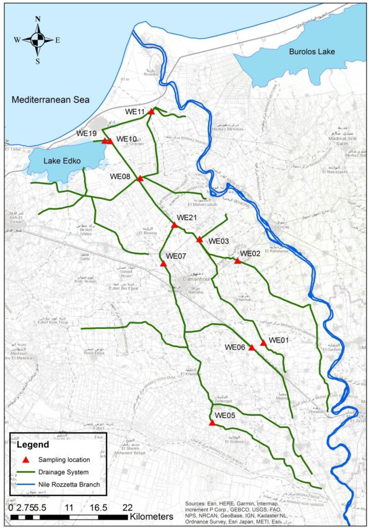
The Edko drainage system is one of the Nile Delta’s major drainage systems. Beginning from Shubra-Kheitto free flow Lake Edko before reaching the Mediterranean, the Edko catchment area is approximately 96,000 hectares with a length of 48.8 km [49]. Since August 1997, monthly samples have been gathered at 11 water quality monitoring locations across the Edko drainage system (Figure 1).
The empirical experiment used ten years of monthly WQ measured records for Sodium (Na) and Total Dissolved Solids (TDS) measured at 10 out of the 11 monitoring locations. One location was excluded due to an incomplete Na dataset. It is assumed that 10 years of monthly records are representative of the Na and TDS measured at these 10 monitoring locations. It should be emphasized that the selection of the Na and TDS for this case study was due to their high correlation.
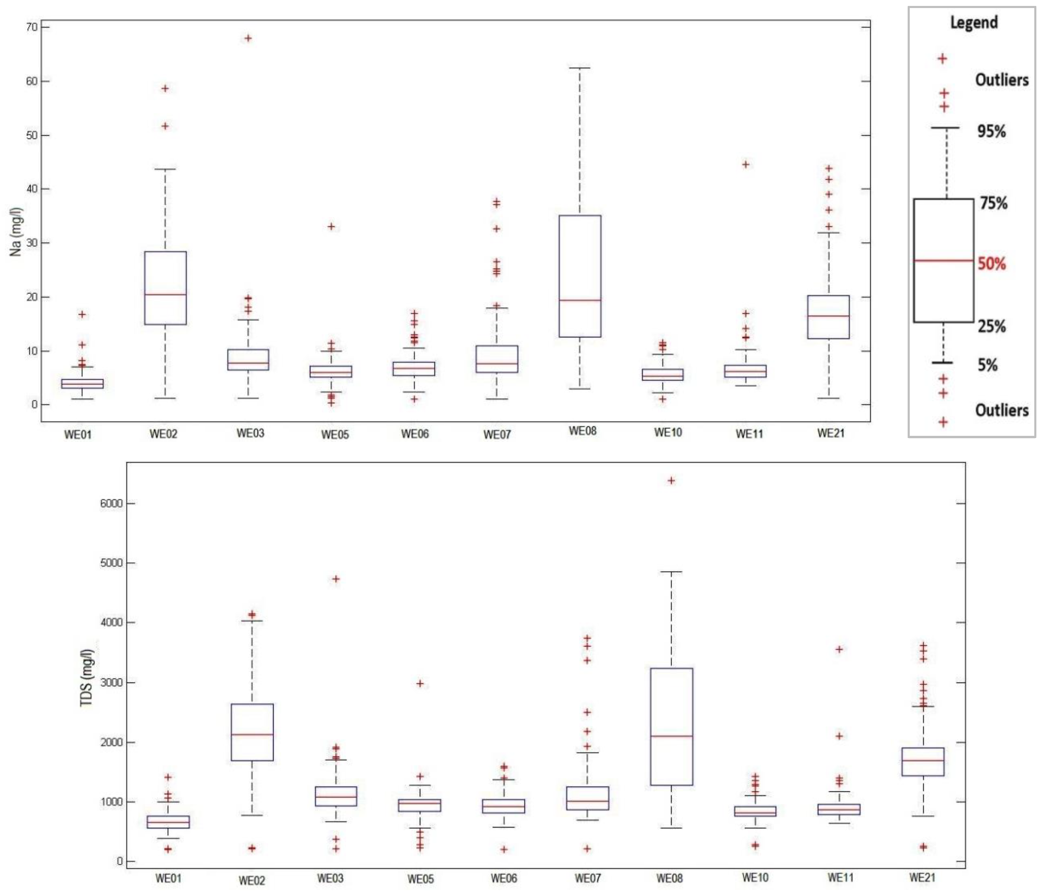
Table 1 shows descriptive statistics for the Na and TDS measured at the 10 monitoring locations. Figure 2 displays the box plots for Na and TDS, which reveal outliers and positive skewness. Table 2 displays the findings of the Kolmogorov–Smirnov goodness-of-fit test, which assesses the normality of the data under the null hypothesis that the sample was drawn from a normal distribution. The results show that none of the two WQ variables at any of the ten monitoring stations allow the test null hypothesis to be accepted (Table 2).
The TDS was employed as an explanatory variable (predictor or independent variable) to extend the Na records (response or dependent variable) using the eight record extension approaches. The effectiveness of the eight record-extension approaches, as well as the use of the À Trous-Haar WT data preprocessing step, were evaluated using a split-sample cross-validation method. In the split sample cross-validation, every two years of monthly records were eliminated from the ten years of available data and the remaining eight years were used to define the period of concurrent records. Four different sizes were considered for the period of concurrent records equal to 60, 70, 80, and 90 records.
The eight record-extension approaches were used for the estimation of Na using TDS as a predictor at each of the Edko drain 10 monitoring locations considered in this study. As a result, 200 different extended Na record realizations were constructed (10 locations × 5 different sample combinations x four different sizes = 200).
For each of the 200 distinct realizations studied, the correlation coefficient of and was consistently positive and ranged between 0.77 and 0.84.
The bias (BIAS) as accuracy metric and the root mean squared error (RMSE) as a precision metric were used to assess the performances of the eight record-extension approaches under the À Trous-Haar data preprocess step:
where and are the measured and estimated statistics of the dependent variable for , respectively, and is the number of trials in the empirical study.
4. Results and Discussion
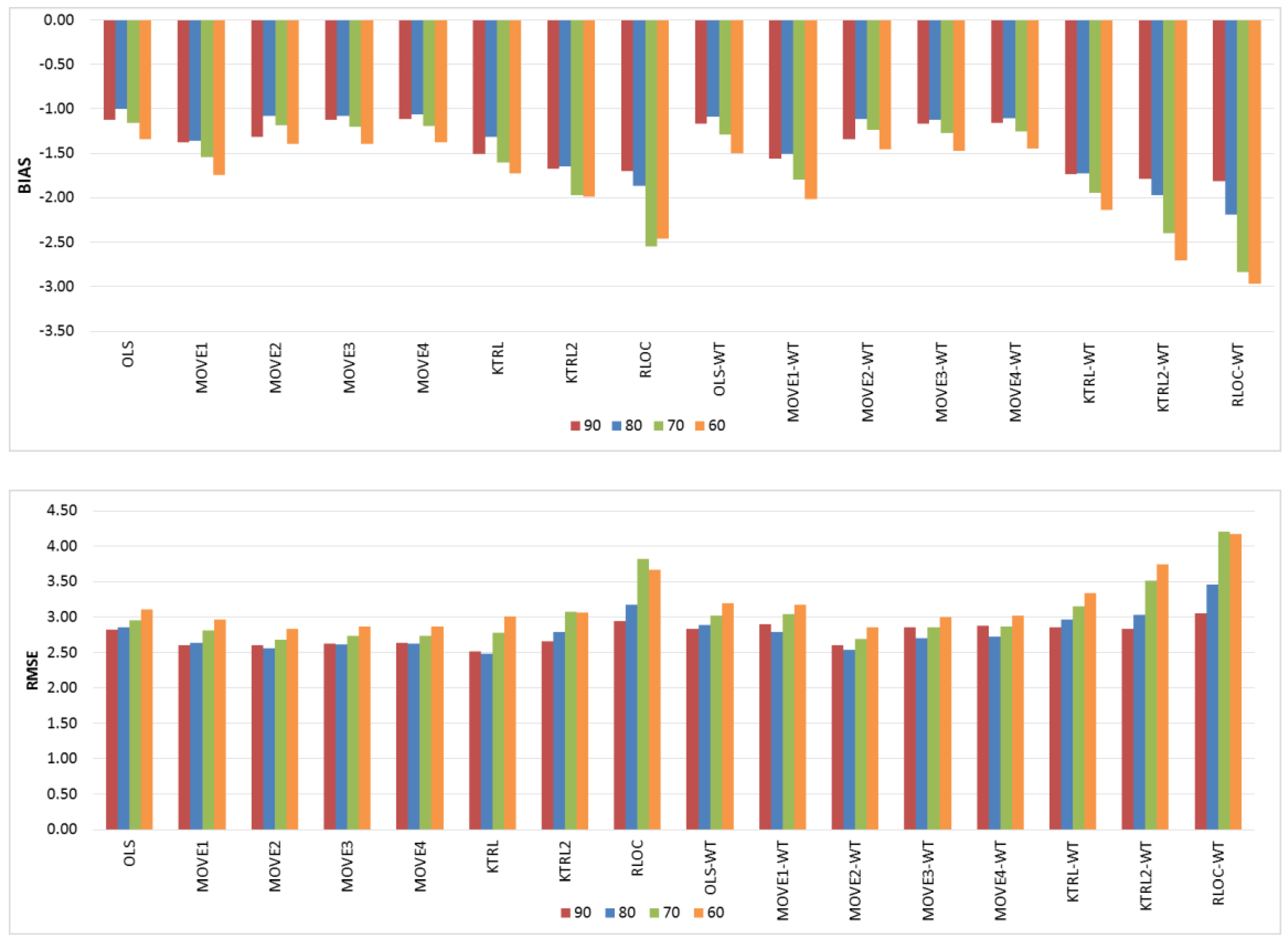
Figure 3, Figure 4 and Figure 5 show the BIAS and RMSE values for the estimation of the extended records (Figure 3), extended records’ mean value (Figure 4), and extended records’ standard deviation (Figure 5).
For the restoration of missing records (Figure 3), the OLS and MOVE techniques showed comparable results, indicating that the WT step had no clear influence. However, for KTRL, KTRL2 and RLOC, the WT step deteriorates the accuracy and precision. These results are due to the high correlation between the two WQ variables (Na & TDS); high linear dependence is one of the assumptions of regression techniques, which may mask the influence of the data preprocessing step for the restoration of a missing record. High precision was generally observed for the KTRL and MOVE techniques, whereas high accuracy was generally observed for OLS, MOVE3, and MOVE4. The KTRL provided the most precise results for the period of concurrent records equal to 90 and 80, whereas MOVE2 was the most precise for concurrent records of sizes equal to 70 and 60. As the period of concurrent records increases, the data become more representative, and nonparametric techniques demonstrated their performance. This dynamic regarding the period of concurrent records is clear not only for the KTRL performance but also for all eight techniques with and without the WT data preprocessing step, as shown in Figure 3.
These results are in agreement with [2] results for the restoration of stream flow missing values, where the use of the À Trous-Haar WT as a preprocessing step did not show consistent improvement. Based on these results and results obtained by [2] and given the limited WQ data (10 years in this study) compared to streamflow data (40 years used by [2]), we may confirm that the use of the À Trous Haar WT as a data preprocessing step did not show clear improvement for the restoration of missing WQ values.
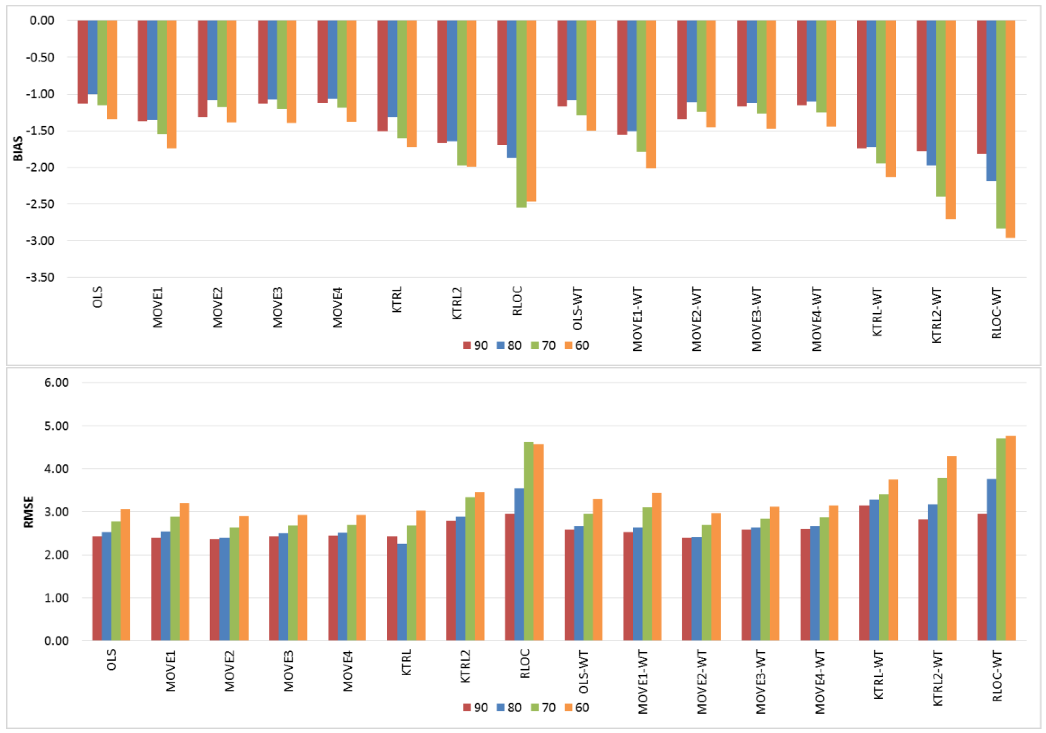
Figure 4 shows the BIAS and RMSE results for the estimation of the mean value of the extended records. In general, the OLS and MOVE techniques showed comparable results with their WT-based counterparts, which indicates that the WT step had no clear influence. However, for KTRL, KTRL2 and RLOC, the WT step deteriorates the accuracy and precision. Given that the regression techniques are proposing a line that passes by the mean (X) and mean (Y) for the OLS, and median (X) and median (Y) for the KTRL, the mean value of the estimated records should be accurate and precise. Given the linear dependence between the TDS and Na, the OLS and MOVE approaches provided more precise and accurate results with almost no influence of the WT data preprocessing step. The period of available records affects more the KTRL, KTRL2, and RLOC approaches; as the period of available records decreases, the accuracy and precision deteriorate. High precision was generally observed for the KTRL, MOVE3, and MOVE4 approaches, whereas high accuracy was generally observed for OLS, MOVE3, and MOVE4.
Figure 5 shows the BIAS and RMSE results for the estimation of the Na expanded records’ standard deviation values. Relatively high accuracy was obtained for the WT-MOVE3, WT-MOVE4, WT-KTRL2 and WT-RLOC techniques, whereas the WT-KTRL2 was the most precise for relatively large-size concurrent records (e.g., n1 = 90), and the WT-MOVE1 provided more precise results for small sizes (e.g., 60 records). Higher accuracy of the extended records’ standard deviation provided by the MOVE3 and MOVE4 approaches than the MOVE1 and MOVE2 is noted. This is attributed to the main difference between those techniques, where MOVE3 and MOVE4 were developed for small-size samples, unlike MOVE1 and MOVE2, which are based on population parameters. These results are in agreement with the results obtained by [10,27], where the four MOVE techniques were compared using streamflow and WQ data, respectively. This indicates the usefulness of the MOVE3 and MOVE4 for such small period of WQ records. The better accuracy provided by the KTRL2, RLOC, WT-KTRL2, and WT-RLOC approaches is due to the advantage of being insensitive to the existence of outliers and the ability to maintain variance of the extended records. These results are in agreement with results obtained by [27,28], which showed the better accuracy and precision provided by the KTRL2 and RLOC compared to MOVE techniques in the presence of outliers. For the extended records’ standard deviation, the WT data preprocessing step smooths the raw data into an approximation component that minimizes the influence of extreme values, which affects the extended records’ variance more than their mean value.
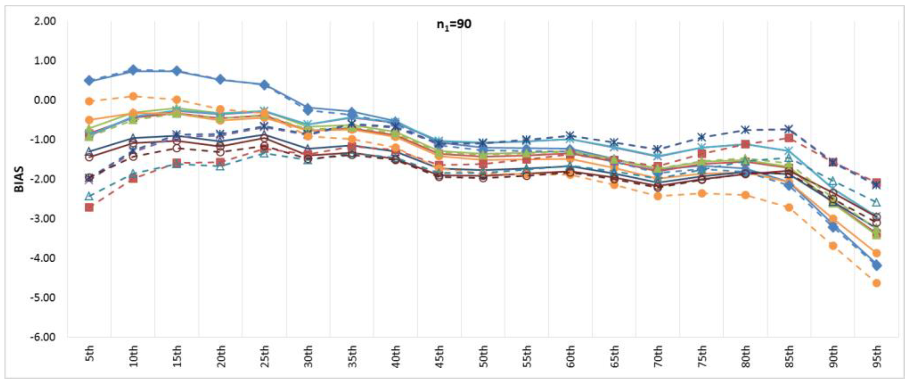
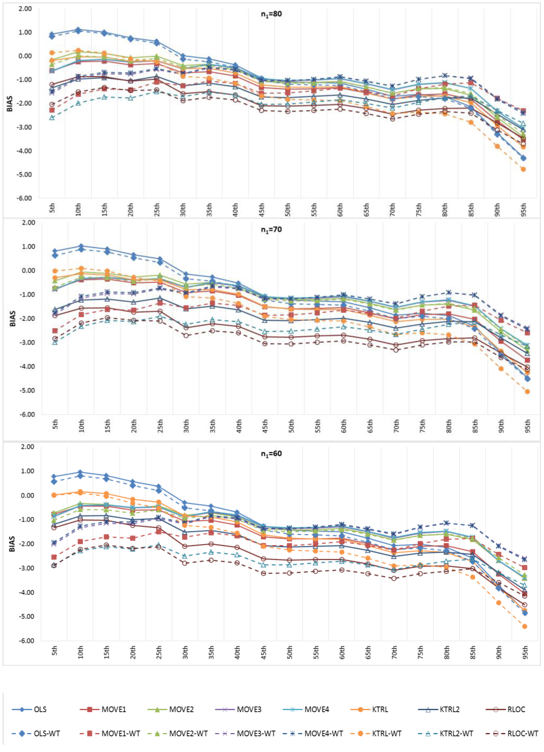
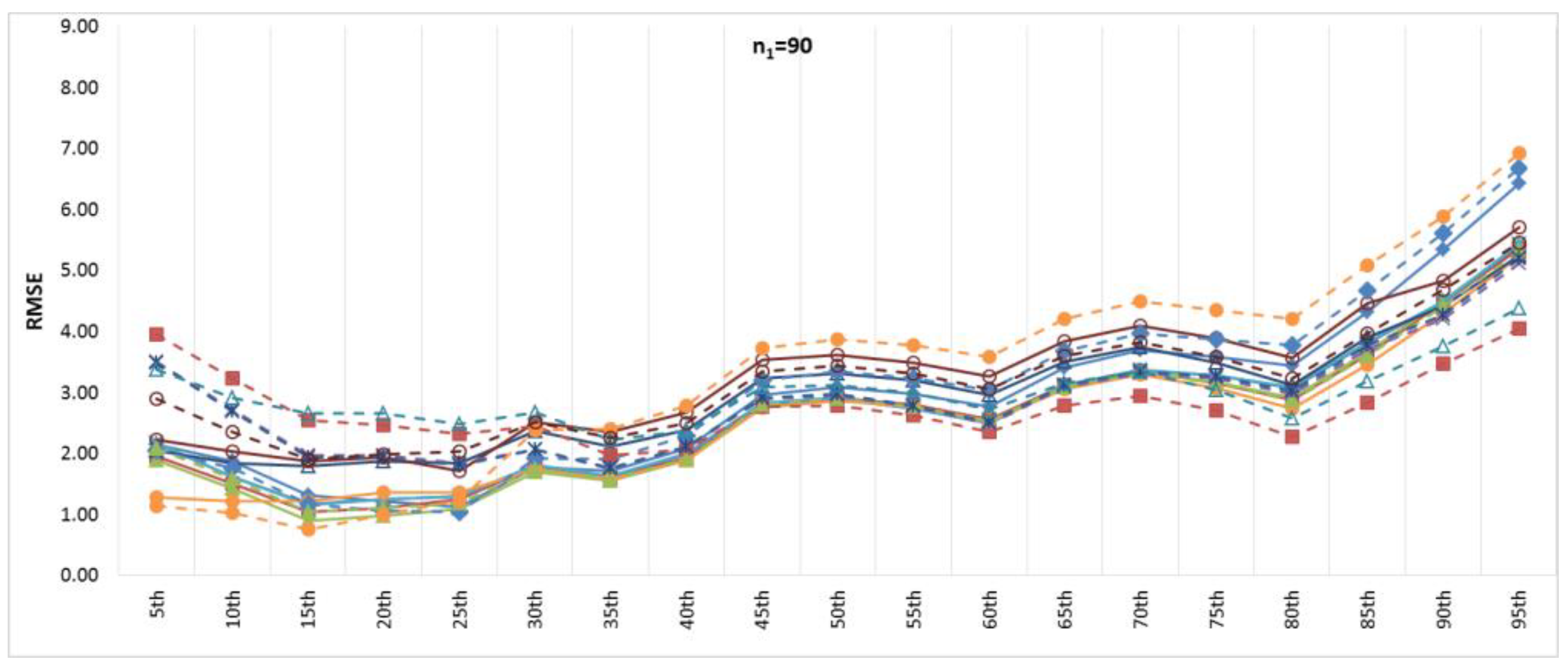
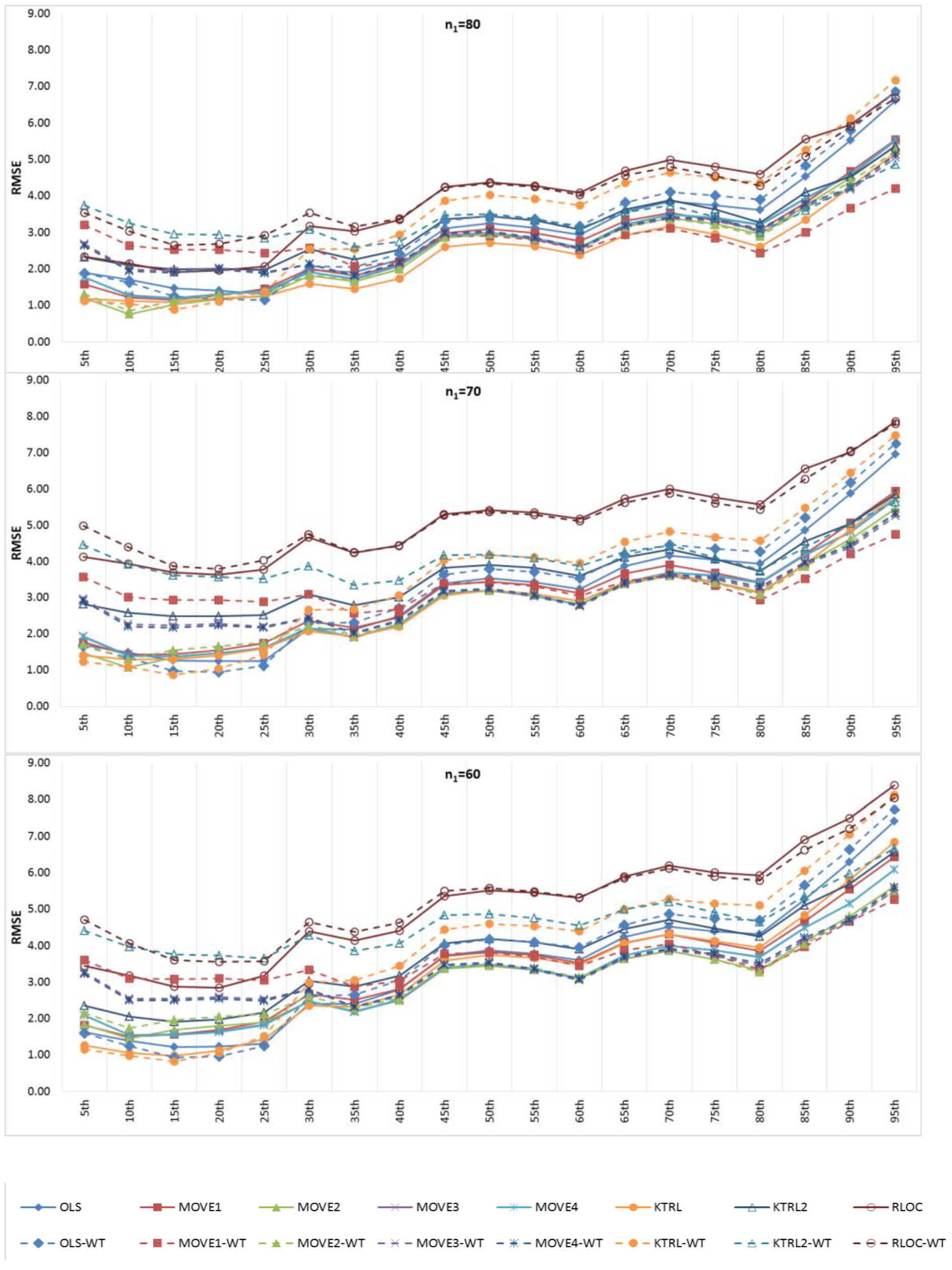
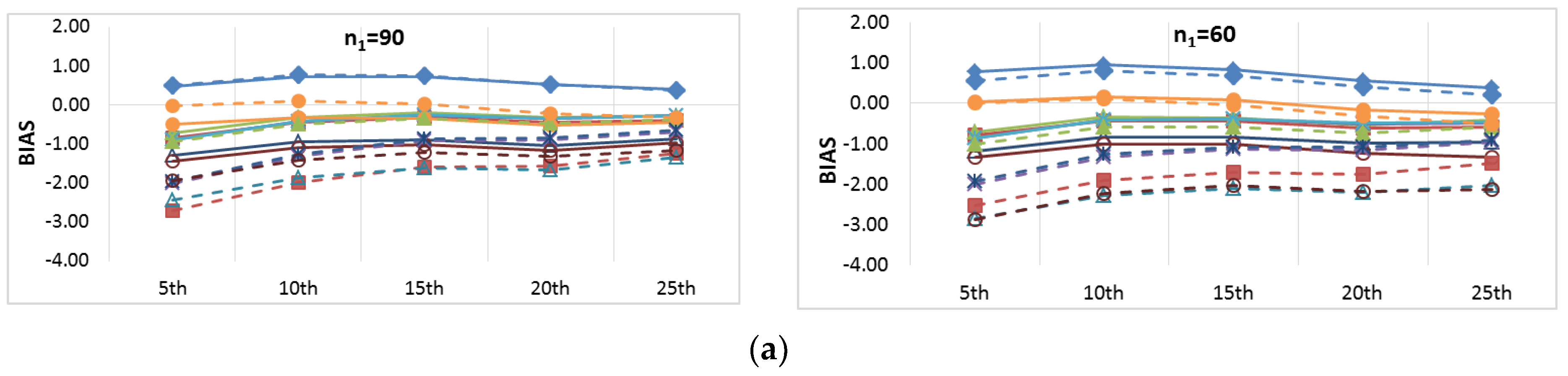
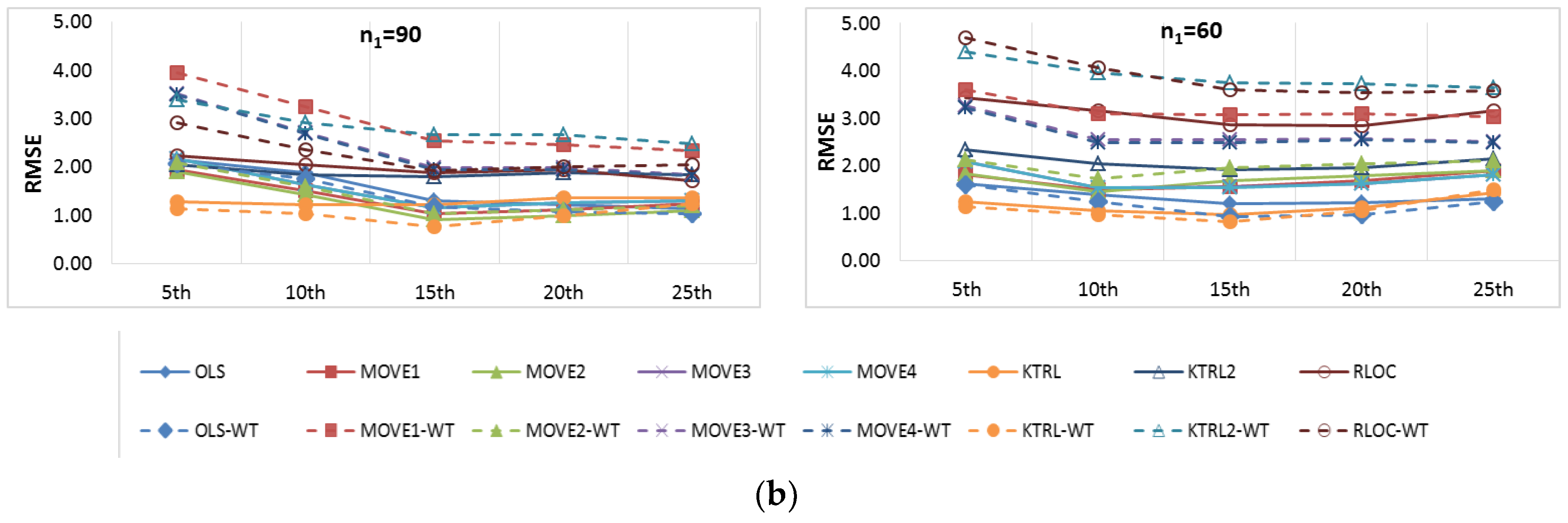
Figure 6 and Figure 7 show the BIAS and RMSE results for the Na extended records’ full length of percentiles from the 5th to the 95th percentile, respectively. Figure 8 and Figure 9 provide more focus on the BIAS and RMSE for the low and high percentiles, respectively. In general, Figure 6, Figure 7, Figure 8 and Figure 9 show that the accuracy and precision of the extended record percentiles increase as the period of concurrent records increases. This is attributed to the first assumption in regression techniques that the dependent and independent data are representative; as the period of concurrent records increases, the data become more representative, and their sample parameters become more accurate and precise.
For the four periods of concurrent records considered, the WT-KTRL provided extended records that are more accurate and precise in presenting the extended period low percentiles. The WT-KTRL showed either similar or slightly better performance than the KTRL. However, for high percentiles (e.g., 85th, 90th and 95th), both the KTRL and WT-KTRL techniques showed the least accuracy and precision (e.g., n1 = 60 and 70) or the second least accuracy and precision for n1 = 80 or 90.
These results are not in agreement with previous results provided by [4], which showed that the KTRL provided extended records that overestimated low percentiles and underestimated high percentiles. These different results are attributed to the existence of outliers in the independent variables (x) more/not in the dependent variable (y), as shown in Figure 2. The heavy existence of outliers in the independent variable relative to the dependent variable affects the variance and standard deviation, which becomes larger than it should be. A clear explanation of the OLS or MOVE1 slope estimates is that an overestimated (fault larger) standard deviation for the independent variable leads to an underestimation of the regression slope. Underestimation of the regression slope provides underestimation of the extended records, which leads to underestimating low as well as high values. For OLS, WT-OLS, KTRL, and WT-KTRL, underestimation of the regression slope leads to reduced overestimation of low values (low percentiles) but simultaneously increases underestimation of high values (high percentiles). Similarly, underestimating the MOVE slope results in underestimating high and low values, resulting in underestimating both high and low percentiles.
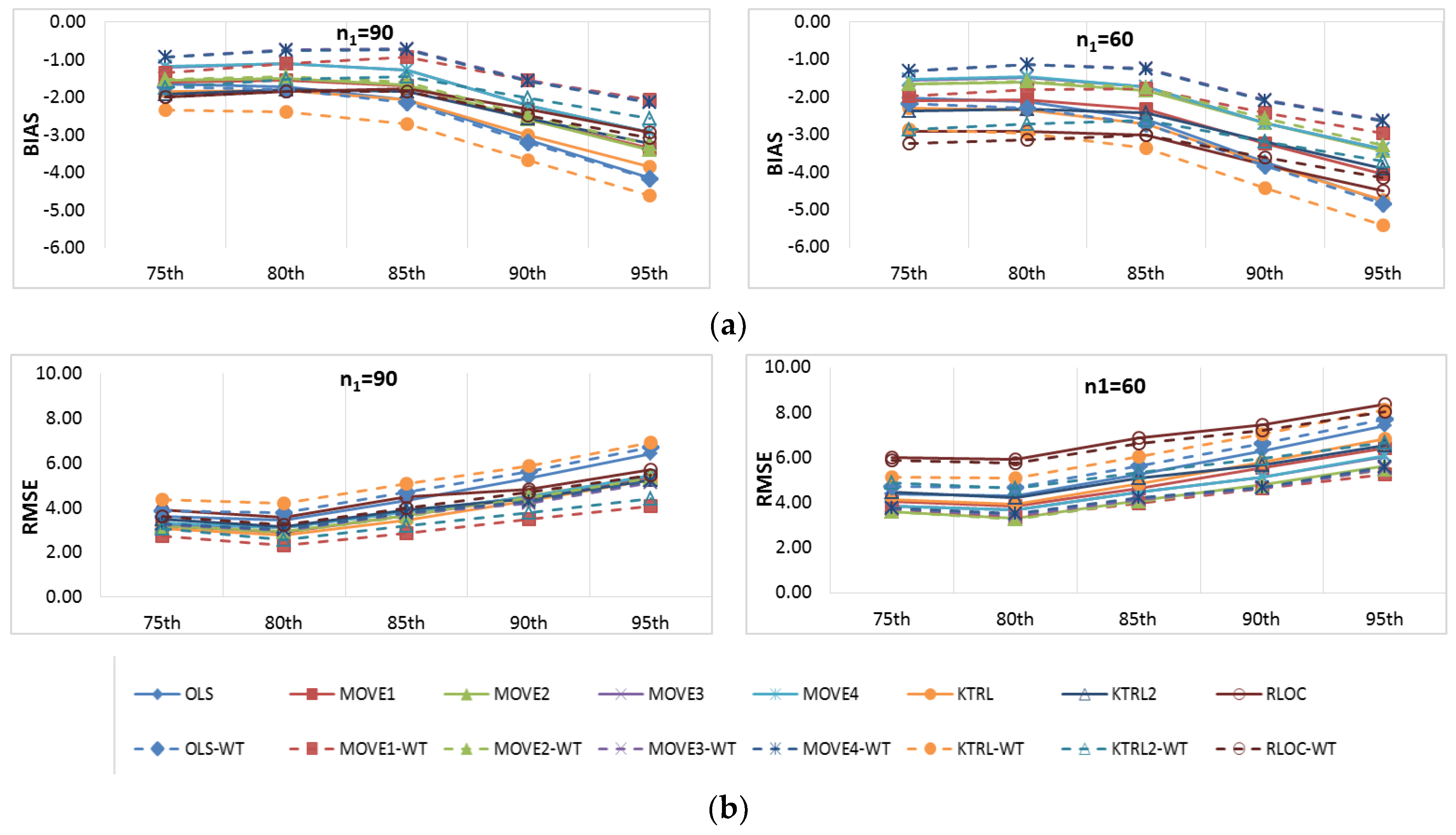
In evaluating the influence of the WT step, WT-KTRL and WT-OLS showed slightly more accurate and precise results than KTRL and OLS, respectively. For the MOVE techniques, for both the high and low percentiles, the WT-step did not show clear improvement but reduced the accuracy and precision. For KTRL2 and RLOC, accuracy and precision improvements were detected with the WT data preprocessing step.
For the four different periods of concurrent records, the highest accuracy in estimating high percentiles was obtained by WT-MOVE3 and WT-MOVE4, followed by the MOVE1-WT technique. The highest precision was obtained by the WT-MOVE1, WT-MOVE3, and WT-MOVE4 techniques, while WT-KTRL2 became the second highest precision technique when the period of concurrent records was 90.
Thus, when the period of concurrent records was large enough to be considered representative, KTRL2 and WT-KTRL2 showed accurate and precise estimates in representing their statistical parameters. However, for restoration of missing records, the KTRL showed more accurate and precise results for small-sample WQ data.
In brief, results showed that using the À Trous-Haar WT as a data preprocessing step did not improve the accuracy or precision of any of the eight regression approaches for the estimation of missing WQ records. However, for the extension of short-gauged WQ records, using the À Trous-Haar WT step improved the accuracy and precision of the extended records’ standard deviation and extreme percentiles. Thus, the use of the À Trous-Haar WT as a data preprocessing step is recommended if the objective is to extend WQ records at short-gauged sites. In addition, and in agreement with previous studies [4,28], results showed that the KTRL is preferable for the restoration of missing WQ values in case of the presence of outliers. For the extension of WQ records, the WT-MOVE3 or WT-MOVE4 is preferable, while in the presence of outliers, the WT-KTRL2 is desirable.
5. Conclusions and Recommendations
For the restoration of WQ missing data and the extension of WQ records at short-gauged locations, eight record-extension strategies were investigated in this study. The evaluation took into account a data preprocessing step that used the À Trous-Haar WT to denoise the predictor by just using the À Trous-Haar approximation component in the regression technique. Real WQ records from the Edko drainage system in Egypt’s Nile Delta were used in an empirical investigation. The results showed that adding the WT data preprocessing step did not improve the restoration of missing values significantly. However, for the extended records’ standard deviation and percentiles, it showed improvements in accuracy and precision.
It can be concluded that the selection of the appropriate record-extension technique is based on two main aspects: the existence of outliers; and the objective of the record substitution, either to estimate missing values or to extend short-gauged records. The existence of outliers should be checked carefully before selecting an applicable record-extension technique, especially if the objective is to provide extended records that preserve the statistical parameters. For the restoration of missing WQ values, either the OLS or the KTRL should be used, with said KTRL being preferred in the existence of outliers. For the extension of WQ records at short-gauged sites, any of the MOVE, KTRL2, or RLOC procedures can be used, with WT-KTRL2 and WT-RLOC preferable in the existence of outliers and WT-MOVE3 and WT-MOVE4 preferable in cases with small sample sizes.
The use of the À Trous-Haar WT as a data preprocessor for record-extension approaches requires more research, including case studies from various regions and an assessment of the impact of outliers, their position, intensity, and magnitudes. Furthermore, analyzing the impact of the period of concurrent records and the level of correlation between the dependent and independent variables on the use of the À Trous-Haar WT as a data preprocessing step would provide a clear assessment. In addition, as a natural extension of this work, other data decomposition techniques such as empirical mode decomposition (EMD) and ensemble EMD (EEMD) (e.g., [50,51,52,53]) would be used instead of WT and would allow comparing different data preprocessing methods.
Author Contributions
Conceptualization, S.A., B.K. and A.E.S.; methodology, S.A., B.K. and A.E.S.; software, S.A. and A.E.; investigation, S.A.; data curation, A.E.S.; writing—original draft preparation, S.A.; writing—review and editing, B.K., A.E.S., A.E. and M.S. All authors have read and agreed to the published version of the manuscript.
Funding
This research received no external funding.
Institutional Review Board Statement
Not applicable.
Informed Consent Statement
Not applicable.
Acknowledgments
The water quality data used in this study were provided by the National Water Research Center (NWRC) of Egypt. The authors are grateful to the Editor, the Associate Editor, and the three anonymous reviewers, whose comments and suggestions greatly improved the quality of the paper.
Conflicts of Interest
The authors declare no conflict of interest.
References
- Halbe, J.; Pahl-Wostl, C.; Sendzimir, J.; Adamowski, J. Towards adaptive and integrated management paradigms to meet the challenges of water governance. Water Sci. Technol. 2013, 67, 2651–2660. [Google Scholar] [CrossRef]
- Nalley, D.; Adamowski, J.; Khalil, B.; Biswas, A. A comparison of conventional and wavelet transform based methods for streamflow record extension. J. Hydrol. 2019, 582, 124503. [Google Scholar] [CrossRef]
- Horne, J. Water Information as a Tool to Enhance Sustainable Water Management—The Australian Experience. Water 2015, 7, 2161–2183. [Google Scholar] [CrossRef] [Green Version]
- Khalil, B.; Ouarda, T.B.M.J.; St-Hilaire, A. Comparison of Record-Extension Techniques for Water Quality Variables. Water Resour. Manag. 2012, 26, 4259–4280. [Google Scholar] [CrossRef]
- Khalil, B.; Adamowski, J. Record extension for short-gauged water quality parameters using a newly proposed robust version of the Line of Organic Correlation technique. Hydrol. Earth Syst. Sci. 2012, 16, 2253–2266. [Google Scholar] [CrossRef] [Green Version]
- Hadzima-Nyarko, M.; Rabi, A.; Šperac, M. Implementation of Artificial Neural Networks in Modeling the Water-Air Temperature Relationship of the River Drava. Water Resour. Manag. 2014, 28, 1379–1394. [Google Scholar] [CrossRef]
- Nevitt, J.; Tam, H.P. A Comparison of Robust and Nonparametric Estimators under the Simple Linear Regression Model. In Proceedings of the Paper presented at the Annual Meeting of the American Educational Research Association, Chicago, IL, USA, 24–28 March 1997. [Google Scholar]
- Granato, G.E. United States, Office of the Natural and Human Environment, Geological Survey (U.S.). In Kendall-Theil Robust Line (KTRLine-Version 1.0): A Visual Basic Program for Calculating and Graphing Robust Nonparametric Estimates of Linear-Regression Coefficients between Two Continuous Variables; Techniques and methods of the, U.S. Geological Survey; Bibliogov: Washington, DC, USA, 2006; Volume 4, p. 31. [Google Scholar]
- Hirsch, R.M. A comparison of four streamflow record extension techniques. Water Resour. Res. 1982, 18, 1081–1088. [Google Scholar] [CrossRef]
- Vogel, R.M.; Stedinger, J.R. Minimum variance streamflow record augmentation procedures. Water Resour. Res. 1985, 21, 715–723. [Google Scholar] [CrossRef] [Green Version]
- Robinson, R.; Wood, M.S.; Smoot, J.L.; Moore, S.E. Parametric modeling of water quality and sampling strategy in a high-altitude appalachian stream. J. Hydrol. 2004, 287, 62–73. [Google Scholar] [CrossRef]
- Koutsoyiannis, D.; Langousis, A. Treatise on Water Science Chapter 27: Precipitation. Treatise Water Sci. 2011, 2, 27–78. [Google Scholar] [CrossRef]
- Canadian Council of Ministers of the Environment. 2015. Available online: https://www.ccme.ca/en/resources/water/water_quality.html (accessed on 1 June 2015).
- Lettenmaier, D.P. Multivariate Nonparametric Tests for Trend in Water Quality. J. Am. Water Resour. Assoc. 1988, 24, 505–512. [Google Scholar] [CrossRef]
- Berryman, D.; Bobee, B.; Cluis, D.; Haemmerli, J. Nonparametric metric tests for trend detection in water quality time series. J. Am. Water Resour. Assoc. 1988, 24, 545–556. [Google Scholar] [CrossRef]
- Dietz, E.J. A comparison of robust estimators in simple linear regression. Commun. Stat. Simul. Comput. 1987, 16, 1209–1227. [Google Scholar] [CrossRef]
- Albek, E. Estimation of point and diffuse contaminant loads to streams by non-parametric regression analysis of monitoring data. Water Air Soil Pollut. 2003, 147, 229–243. [Google Scholar] [CrossRef]
- Olsson, O.; Gassmann, M.; Wegerich, K.; Bauer, M. Identification of the effective water availability from streamflows in the Zerafshan river basin, Central Asia. J. Hydrol. 2010, 390, 190–197. [Google Scholar] [CrossRef]
- Dery, S.J.; Mlynowski, T.J.; Hernandez-Henriquez, M.A.; Straneo, F. Interannual variability and interdecadal trends in Hudson Bay streamflow. J. Mar. Syst. 2011, 88, 341–351. [Google Scholar] [CrossRef]
- Vorogushyn, S.; Merz, B. Flood trends along the Rhine: The role of river training. Hydrol. Earth Syst. Sci. 2013, 17, 3871–3884. [Google Scholar] [CrossRef] [Green Version]
- Calarullo, S.J.; Sullivan, S.L.; McHugh, A.R. Implementation of MOVE.1, Censored MOVE.1, and Piecewise MOVE.1 Low-Flow Regressions with Applications at Partial-Record Streamgaging Stations in New Jersey: U.S. Geological Survey Open-File Report 2018-1089. 20p. Available online: https://pubs.usgs.gov/of/2018/1089/ofr20181089.pdf (accessed on 6 November 2018).
- Jia, Y.; Culver, T.B. Bootstrapped artificial neural networks for synthetic flow generation with a small data sample. J. Hydrol. 2006, 331, 580–590. [Google Scholar] [CrossRef]
- Ryu, J.H.; Svoboda, M.D.; Lenters, J.D.; Tadesse, T.; Knutson, C.L. Potential extents for ENSO-driven hydrologic drought forecasts in the United States. Clim. Chang. 2009, 101, 575–597. [Google Scholar] [CrossRef]
- Raziei, T.; Saghafian, B.; Paulo, A.A.; Pereira, L.S.; Bordi, I. Spatial Patterns and Temporal Variability of Drought in Western Iran. Water Resour. Manag. 2008, 23, 439–455. [Google Scholar] [CrossRef] [Green Version]
- Raziei, T.; Bordi, I.; Pereira, L.S. An application of GPCC and NCEP/NCAR datasets for draught variability analysis in Iran. Water Resour. Manag. 2011, 25, 1075–1086. [Google Scholar] [CrossRef]
- Khalil, B.; Awadallah, A.G.; Adamowski, J.; Elsayed, A. A Novel Record-Extension Technique for Water Quality Variables Based on L-Moments. Water Air Soil Pollut. 2016, 227, 179. [Google Scholar] [CrossRef]
- Khalil, B.; Adamowski, J. Comparison of OLS, ANN, KTRL, KTRL2, RLOC, and MOVE as record-extension techniques for water quality variables. Water Air Soil Pollut. 2014, 225, 1966. [Google Scholar] [CrossRef]
- Khalil, B.; Adamowski, J. Evaluation of the performance of eight record-extension techniques under different levels of association, presence of outliers and different sizes of concurrent records: A Monte Carlo study. Water Resour. Manag. 2014, 28, 5139–5155. [Google Scholar] [CrossRef]
- Helsel, D.; Hirsch, R.M. Statistical Methods in Water Resources (USGS Numbered Series No. 04-A3), Statistical Methods in Water Resources, Techniques of Water-Resources Investigations; U.S. Geological Survey: Reston, VA, USA, 2002. [Google Scholar] [CrossRef]
- Draper, N.R.; Smith, H. Applied Regression Analysis; John Wiley: New York, NY, USA, 1966; 736p. [Google Scholar]
- Serinaldi, F.; Grimaldi, S.; Abdolhosseini, M.; Corona, P.; Cimini, D. Testing copula regression against benchmark models for point and interval estimation of tree wood volume in beech stands. Forstwiss. Centralblatt 2012, 131, 1313–1326. [Google Scholar] [CrossRef] [Green Version]
- Moog, D.B.; Whiting, P.J.; Thomas, R.B. Streamflow record extension using power transformations and application to sediment transport. Water Resour. Res. 1999, 35, 243–254. [Google Scholar] [CrossRef]
- Matalas, N.; Jacobs, B. A Correlation Procedure for Augmenting Hydrologic Data; (USGS Numbered Series No. 434-E), a Correlation Procedure for Augmenting Hydrologic Data, Professional Paper; U.S. Government Printing Office: Washington, DC, USA, 1964. [Google Scholar] [CrossRef]
- Theil, H. A rank-invariant method of linear and polynomial regression analysis I and II. Indag. Math. 1950, 12, 173. [Google Scholar]
- Groeneveld, R.A.; Conover, W.J. Practical Nonparametric Statistics, 2nd ed.; John Wiley and Sons: New York, NY, USA, 1980; 493p. [Google Scholar]
- Partal, T.; Kişi, Ö. Wavelet and neuro-fuzzy conjunction model for precipitation forecasting. J. Hydrol. 2007, 342, 199–212. [Google Scholar] [CrossRef]
- Partal, T.; Cigizoglu, K. Estimation and forecasting of daily suspended sediment data using wavelet-neural networks. J. Hydrol. 2008, 358, 317–331. [Google Scholar] [CrossRef]
- Adamowski, J.; Chan, H.F. A wavelet neural network conjunction model for groundwater level forecasting. J. Hydrol. 2011, 407, 28–40. [Google Scholar] [CrossRef]
- Pandey, B.K.; Tiwari, H.; Khare, D. Trend analysis using discrete wavelet transform (DWT) for long-term precipitation (1851–2006) over India. Hydrol. Sci. J. 2017, 62, 2187–2208. [Google Scholar] [CrossRef]
- Graf, R.; Zhu, S.; Sivakumar, B. Forecasting river water temperature time series using a wavelet–neural network hybrid modelling approach. J. Hydrol. 2019, 578, 124115. [Google Scholar] [CrossRef]
- Liu, Q.-J.; Shi, Z.-H.; Fang, N.-F.; Zhu, H.-D.; Ai, L. Modeling the daily suspended sediment concentration in a hyperconcentrated river on the Loess Plateau, China, using the Wavelet–ANN approach. Geomorphology 2013, 186, 181–190. [Google Scholar] [CrossRef]
- Tiwari, M.K.; Chatterjee, C. A new wavelet–bootstrap–ANN hybrid model for daily discharge forecasting. J. Hydroinform. 2010, 13, 500–519. [Google Scholar] [CrossRef] [Green Version]
- Mallat, S. A Wavelet Tour of Signal Processing, 2nd ed.; Academic Press: San Diego, CA, USA, 1999. [Google Scholar]
- Du, K.; Zhao, Y.; Lei, J. The incorrect usage of singular spectral analysis and discrete wavelet transform in hybrid models to predict hydrological time series. J. Hydrol. 2017, 552, 44–51. [Google Scholar] [CrossRef]
- Renaud, O.; Starck, J.-L.; Murtagh, F. Wavelet-Based Combined Signal Filtering and Prediction. IEEE Trans. Syst. Man Cibern. Part B 2005, 35, 1241–1251. [Google Scholar] [CrossRef]
- Shensa, M. The discrete wavelet transform: Wedding the a trous and Mallat algorithms. IEEE Trans. Signal Process. 1992, 40, 2464–2482. [Google Scholar] [CrossRef] [Green Version]
- Zheng, G.; Starck, J.-L.; Campbell, J.; Murtagh, F. Multiscale transforms for filtering financial data streams. J. Comput. Intell. Financ. 1999, 7, 18–35. [Google Scholar]
- Murtagh, F.; Starck, J.L.; Renaud, O. On neuro-wavelet modeling. Decis. Support Syst. 2004, 37, 475–484. [Google Scholar] [CrossRef]
- El-Saadi, A. Economics and Uncertainty Considerations in Water Quality Monitoring Networks Design. Ph.D. Dissertation, Faculty of Engineering, Ain-Shams University, Cairo, Egypt, 2006. [Google Scholar]
- Huang, N.E.; Shen, Z.; Long, S.R.; Wu, M.C.; Shih, H.H.; Zheng, Q.; Yen, N.-C.; Tung, C.C.; Liu, H.H. The empirical mode decomposition and the Hilbert spectrum for nonlinear and non-stationary time series analysis. Proc. R. Soc. Lond. Ser. A Math. Phys. Eng. Sci. 1998, 454, 903–995. [Google Scholar] [CrossRef]
- Nelsen, B.; Williams, D.A.; Williams, G.P.; Berrett, C. An Empirical Mode-Spatial Model for Environmental Data Imputation. Hydrology 2018, 5, 63. [Google Scholar] [CrossRef] [Green Version]
- Eze, E.; Halse, S.; Ajmal, T. Developing a Novel Water Quality Prediction Model for a South African Aquaculture Farm. Water 2021, 13, 1782. [Google Scholar] [CrossRef]
- Chu, T.-Y.; Huang, W.-C. Application of Empirical Mode Decomposition Method to Synthesize Flow Data: A Case Study of Hushan Reservoir in Taiwan. Water 2020, 12, 927. [Google Scholar] [CrossRef] [Green Version]
Figure 1.
Edko drainage system WQ monitoring locations.

Figure 2.
Box plots for the Na and TDS records.

Figure 3.
The BIAS and RMSE results for the extended Na records for four different periods of concurrent records = 60; 70; 80; and 90.
Figure 3.
The BIAS and RMSE results for the extended Na records for four different periods of concurrent records = 60; 70; 80; and 90.

Figure 4.
The BIAS and RMSE results for the extended Na records mean value for four different periods of concurrent records = 60; 70; 80; and 90.
Figure 4.
The BIAS and RMSE results for the extended Na records mean value for four different periods of concurrent records = 60; 70; 80; and 90.

Figure 5.
The BIAS and RMSE results for the extended Na records standard deviation for four different concurrent sizes = 60; 70; 80; and 90.
Figure 5.
The BIAS and RMSE results for the extended Na records standard deviation for four different concurrent sizes = 60; 70; 80; and 90.

Figure 6.
The BIAS results for the extended Na records’ percentiles.


Figure 7.
The RMSE results for the extended Na records’ percentiles.


Figure 8.
The BIAS (a) and RMSE (b) results for the extended Na records’ low percentiles for n1 = 60 and 90.
Figure 8.
The BIAS (a) and RMSE (b) results for the extended Na records’ low percentiles for n1 = 60 and 90.


Figure 9.
The BIAS (a) and RMSE (b) results for the extended Na records’ high percentiles for n1 = 60 and 90.
Figure 9.
The BIAS (a) and RMSE (b) results for the extended Na records’ high percentiles for n1 = 60 and 90.


Table 1.
Na and TDS descriptive statistics.
| Monitoring Locations | Minimum | Maximum | Mean | St. Deviation | Skewness | |||||
|---|---|---|---|---|---|---|---|---|---|---|
| Na | TDS | Na | TDS | Na | TDS | Na | TDS | Na | TDS | |
| (mg/l) | ||||||||||
| WE01 | 1.13 | 203.00 | 16.79 | 1411.00 | 4.14 | 667.99 | 1.96 | 179.36 | 2.84 | 0.61 |
| WE02 | 1.20 | 216.00 | 58.71 | 4155.61 | 21.45 | 2138.95 | 10.40 | 772.74 | 0.52 | 0.16 |
| WE03 | 1.16 | 213.00 | 68.02 | 4734.70 | 9.17 | 1118.71 | 6.57 | 450.35 | 6.38 | 4.46 |
| WE05 | 0.31 | 232.00 | 33.05 | 2978.05 | 6.31 | 950.24 | 3.09 | 266.01 | 5.61 | 3.43 |
| WE06 | 1.09 | 197.00 | 16.96 | 1602.07 | 7.01 | 946.12 | 2.51 | 207.51 | 1.31 | 0.43 |
| WE07 | 1.13 | 210.00 | 37.71 | 3737.00 | 9.47 | 1141.43 | 6.14 | 514.64 | 2.66 | 2.97 |
| WE08 | 3.00 | 562.00 | 62.41 | 6390.00 | 23.73 | 2313.47 | 14.24 | 1153.32 | 0.66 | 0.64 |
| WE10 | 1.00 | 259.00 | 11.61 | 1426.00 | 5.70 | 835.95 | 1.88 | 168.32 | 0.86 | 0.41 |
| WE11 | 3.52 | 642.00 | 44.53 | 3556.00 | 6.78 | 913.38 | 4.14 | 306.54 | 6.86 | 6.20 |
| WE21 | 1.27 | 232.00 | 43.88 | 3624.00 | 17.36 | 1774.25 | 7.91 | 577.39 | 0.98 | 0.82 |
Table 2.
Kolmogorov–Smirnov goodness of fit test for Na and TDS.
| Monitoring Locations | p Value | |
|---|---|---|
| Na | TDS | |
| WE01 | 3.35 × 10−91 | 1.80 × 10−102 |
| WE02 | 6.03 × 10−99 | 1.80 × 10−102 |
| WE03 | 5.76 × 10−96 | 1.80 × 10−102 |
| WE05 | 4.71 × 10−94 | 1.80 × 10−102 |
| WE06 | 3.19 × 10−99 | 1.80 × 10−102 |
| WE07 | 6.58 × 10−99 | 1.80 × 10−102 |
| WE08 | 3.40 × 10−102 | 1.80 × 10−102 |
| WE10 | 8.20 × 10−97 | 1.80 × 10−102 |
| WE21 | 6.03 × 10−99 | 1.80 × 10−102 |
| WE11 | 2.00 × 10−102 | 1.80 × 10−102 |
| WE21 | 6.03 × 10−99 | 1.80 × 10−102 |
Publisher’s Note: MDPI stays neutral with regard to jurisdictional claims in published maps and institutional affiliations. |
© 2022 by the authors. Licensee MDPI, Basel, Switzerland. This article is an open access article distributed under the terms and conditions of the Creative Commons Attribution (CC BY) license (https://creativecommons.org/licenses/by/4.0/).
Share and Cite
MDPI and ACS Style
Anwar, S.; Khalil, B.; Seddik, M.; Eltahan, A.; Saadi, A.E. An Evaluation of À Trous-Based Record Extension Techniques for Water Quality Record Extension. Water 2022, 14, 2264. https://doi.org/10.3390/w14142264
AMA Style
Anwar S, Khalil B, Seddik M, Eltahan A, Saadi AE. An Evaluation of À Trous-Based Record Extension Techniques for Water Quality Record Extension. Water. 2022; 14(14):2264. https://doi.org/10.3390/w14142264
Chicago/Turabian StyleAnwar, Samah, Bahaa Khalil, Mohamed Seddik, Abdelhamid Eltahan, and Aiman El Saadi. 2022. "An Evaluation of À Trous-Based Record Extension Techniques for Water Quality Record Extension" Water 14, no. 14: 2264. https://doi.org/10.3390/w14142264
Note that from the first issue of 2016, this journal uses article numbers instead of page numbers. See further details here.