
Land Cover Change Effects on Stormflow Characteristics across Broad Hydroclimate Representative Urban Watersheds in the United States


1
ASRC Federal Data Solutions, Sioux Falls, SD 57198, USA
2
U.S. Geological Survey (USGS) Earth Resources Observation and Science (EROS) Center, Sioux Falls, SD 57198, USA
3
North Central Climate Adaptation Science Center, Fort Collins, CO 80523, USA
*
Author to whom correspondence should be addressed.
Water 2022, 14(14), 2256; https://doi.org/10.3390/w14142256
Submission received: 23 June 2022
/
Revised: 11 July 2022
/
Accepted: 15 July 2022
/
Published: 19 July 2022
(This article belongs to the Special Issue Ecohydrological Response to Environmental Change)
Abstract
:Urban development alters stormflow characteristics and is associated with increasing flood risks. The long-term evaluation of stormflow characteristics that exacerbate floods, such as peak stormflow and time-to-peak stormflow at varying levels of urbanization across different hydroclimates, is limited. This study investigated the long-term (1980s to 2010s) effects of increasing urbanization on key stormflow characteristics using observed 15 min streamflow data across six broad hydroclimate representative urban watersheds in the conterminous United States. The results indicate upward trends in peak stormflow and downward trends in time-to-peak stormflow at four out of six watersheds. The watershed in the Great Plains region had the largest annual increasing (decreasing) percent change in peak stormflow (time-to-peak stormflow). With the current change rates, peak stormflow in the Great Plains region watershed is expected to increase by 55.4% and have a 2.71 h faster time-to-peak stormflow in the next decade.
1. Introduction
The quantification of streamflow responses to rapidly changing land cover is critical, especially in developing urban areas where floods result in devastating consequences to lives and the economy around the world [1,2,3]. Urbanization lowers soil infiltration rates and channels more water from precipitation to surface runoff, creating more favorable conditions for flooding and subsequently altering streamflow responses [4,5]. Floods were ranked as the third deadliest hazard worldwide over the past 50 years (1970–2019) in a report by the World Meteorological Organization [1]. With increasing urban developments and an increasing proportion of population exposure to floods [6], close monitoring of the urban growth and hydrological flux that exacerbates floods is important.
Streamflow from a watershed includes baseflow and stormflow. Baseflow is underground water flow through saturated soil or groundwater with a relatively slow velocity, whereas stormflow is typically quick overland flow with higher volume, potentially leading to devastating floods following major precipitation events. Several studies have reported varying magnitudes of streamflow changes depending on different levels of urban development [5,7,8,9,10,11,12]. The hydrologic impacts of increasing urbanization are known for increasing stormwater runoff volume, increasing peak flows, and decreasing flow times [13,14,15]. A study at three different levels of urban development reported a larger annual stormflow volume in a high urbanized watershed compared to that in a low urbanized watershed [16]. Increases in peak stormflow and decreases in time-to-peak stormflow associated with increasing urbanization have been reported in event scale studies [13,14,17]. However, the rate of change in peak and time-to-peak is unique to each watershed, and the rates of change derived from event scale studies could vary over a long period of time. Long-term interannual evaluations at several watersheds with varying levels of urbanization across different hydroclimate are limited. A long-term observation-based study in the eastern United States (Washington, DC) reported higher annual stormflow discharge from an urban watershed than those from non-urban watersheds [18]. Extension of such studies at several watersheds with varying levels of urbanization provides detailed information, including variations in overall trends and interannual change rates of key stormflow characteristics (peak and time-to-peak) across different hydroclimate regions. The current study tries to explore these with observed streamflow data as a real case study.
Historical land cover data for the United States was scarce until the recent publication of annual land cover maps from the Land Change Monitoring, Assessment, and Projection (LCMAP) [19,20]. The continuous long-term (1985–2020) land cover data from LCMAP provides an opportunity to evaluate the long-term interannual effects of urban development on stormflow characteristics. Additionally, the near-instantaneous (15 min) streamflow data of numerous streamgages by the U.S. Geological Survey (USGS) are unparalleled for monitoring the changes in stormflow characteristics at a finer temporal scale. Taking advantage of these datasets, quantification of changes in stormflow characteristics, specifically those that are associated with urban floods, such as peak stormflow and time-to-peak stormflow, provides important information for understanding the linkage with changes in urban developments and for practical applications, including designing urban stormwater management infrastructures.
With increasing urban developments, the stormflow characteristics from urban watersheds are expected to have increasing peak stormflows and decreasing time-to-peak stormflows [13,14,17]. The expected long-term effects and the extent of these changes, however, may vary with the levels of urbanization of watersheds, implementation of urban stormwater management infrastructures, and hydroclimate. The main aim of the study was to investigate the long-term annual scale effects of urbanization on key stormflow characteristics (peak stormflow and time-to-peak stormflow) by generating a series of unit hydrographs (UHs) and quantifying the changes in UHs (described in Section 2.3) of six representative urban watersheds across six broad hydroclimate regions across the conterminous United States.
2. Data and Methods
2.1. Selection of Urban Watersheds
Six representative urban watersheds were selected across six broad hydroclimate regions [21] of the conterminous United States (Figure 1). At each hydroclimate region, a watershed was selected which met the following criteria: (i) largest increase in urban area percent between 1985 and 2019, (ii) long-term (>15 years) near-instantaneous (15 min) streamflow data between 1985 and 2019, (iii) relatively small (<200 km2) watersheds assuming a more uniform rainfall distribution for generating unit hydrographs (UHs), and (iv) less than 1% watershed area as open water to exclude potential large lakes and reservoirs that could alter natural stormflow characteristics. The watersheds meeting these criteria are generally located in the suburbs of the major cities (Figure 1). The boundaries of the watersheds were delineated by applying digital elevation model 30 m maps [22] in ArcMap version 10.7.1 (Esri Inc., West Redlands, CA, USA). The areas of the watersheds range from 54.5 km2 to 197.6 km2, with an average of 135.8 km2 (Table 1).
2.2. Streamflow and Land Cover Data
For generation of UHs, near-instantaneous (15 min) streamflow data were obtained from the USGS National Water Information System [23]. The selected watersheds have streamflow data starting as early as the late 1980s (Midwest region watershed), although most of them start during or after the 1990s (Table 1). Land cover data were obtained from the LCMAP Collection 1.1 [19,20]. The LCMAP has a suite of 10 science products including the primary land cover with 8 land cover types (Figure 1d) for the conterminous United States. The primary land cover maps were used to generate annual time series of urban (developed) area percent and increase in urban areas during the study period at six watersheds. Although LCMAP data were available since 1985, streamflow data were only available from the late 1990s or early 2000s for most of the watersheds (Table 1). Thus, the start study years and study period (18 to 30 years) varied across study watersheds based on the availability of streamflow data.
2.3. Generation of Unit Hydrographs
The unit hydrograph of a watershed is defined as the direct runoff (total streamflow minus baseflow) resulting from a unit (e.g., 1 mm) of excess rainfall generated uniformly over the watershed area during a specified time. The event scale UHs generated from observed data, such as the USGS streamgage data applied in this study, reflect the characteristics of both watershed and rainfall. To reduce the influence of rainfall characteristics, several event scale UHs for a given year were averaged to represent the specific year at each watershed [24]. Thus, the interannual changes in average UH characteristics (peak and time-to-peak) can be attributed to changes in land cover, considering that other watershed physical characteristics (e.g., topography, river/stream network, slope, and soil type) remain unchanged.
The first step for the generation of event scale UHs requires the separation of stormflow from streamflow for those events with reasonably clean rising and falling limbs, i.e., not contaminated by previous or following flow events [25]. Upon visual inspection of such clean storm events, the constant slope method [26] was applied to separate stormflow from streamflow by using the Hydrograph-py version 1.0.1 Python package [27]. The slope recommended by the constant slope method’s original authors [26] was too steep for the watersheds in this study. Thus, the slope was reduced to 1.83 L s−1 km−2 d−1, as suggested and implemented in previous studies [28,29]. To include the stormflows generated from more uniform precipitation over the entire area of watersheds, only stormflow events that lasted for more than four hours were considered. The stormflow (m3 s−1) was divided by excess runoff (total stormflow volume from each event divided by watershed area) to compute the ordinates of UHs in the units of m3 s−1 mm−1. For further refinement for reducing the influence of rainfall characteristics, the UHs with peak (m3 s−1 mm−1) and time-to-peak (hour) values above the 90th percentile and below the 10th percentile for each year (January–December) were excluded. The retained event scale UHs for each year were then averaged to obtain an average UH representing that specific year. This process was repeated for all study years at all watersheds to generate several average UHs to quantify the peak and time-to-peak of UHs representing the peak stormflow and time-to-peak stormflow, respectively. The minimum number of stormflow events for a given year was determined using a threshold of mean number of stormflow events for all years minus one standard deviation; years with fewer stormflow events were excluded from the analysis.
2.4. Analysis
Changes in streamflow characteristics and land cover were conducted by trend analysis using the ordinary least squares regression during the study years at each watershed. If the urban area (% of watershed area) changed significantly (p-value ≤ 0.05) during the study years, then any changes or trends in stormflow characteristics were considered to be affected by changes in land cover. For practical applications, the quantification of expected increase or decrease in peak stormflow and time-to-peak stormflow due to a unit increase in excess rainfall is useful for designing stormwater management infrastructures. Therefore, the annual percent changes in peak stormflow and time-to-peak stormflow were computed as a ratio of the slopes of regression lines divided by their respective average values during the study years. Based on the slopes of regression lines, the expected increase or decrease in peak stormflow and expected faster or slower time-to-peak stormflow in a decade (10 years) are computed. The supporting data for this study are publicly available as a USGS data release [30].
3. Results and Discussion
3.1. Changes in Urban Area
The long-term (1985–2019) changes in land cover at all watersheds are shown in Figure 2. Large increases in urban areas occurred in the 1990s and 2000s in most of the watersheds. The selected six watersheds have varying levels of urbanization, at between 10.7% (start study year at the West region watershed) and 73.1% (end study year at the Pacific Northwest region watershed) (Figure 1). Relatively lesser percentages of urban areas in the Great Plains (<33%) and West region (<12%) watersheds are due to the filters applied in this study (see Section 2.1). The increase in urban area percentages, during the study period, for the Northeast, Southeast, Midwest, Great Plains, West, and Pacific Northwest regions were 15.1% (29.8 km2), 10.2% (8.2 km2), 20.3% (11.1 km2), 0.7% (1.1 km2), and 5.3% (8.7 km2), respectively (Figure 2). Among the six watersheds, four watersheds in the Central and Eastern regions of the United States had relatively large (>10%) increases in urban areas. The watersheds in the Northeast and Southeast regions had large area conversion from cropland or tree cover to an urban environment, resulting in the dominant land cover as urban (>60% of the watershed area) in 2019 (Figure 1). The two watersheds in the Midwest and Great Plains regions had increases in urban areas primarily from croplands, and croplands remained the dominant land cover (>48% of the watershed area) in 2019. The two watersheds in the West and Northwest Pacific regions had relatively less (<6%) of an increase in urban areas, with the respective dominant land covers as tree cover (62.3% of the watershed area) and urban (72.5% of the watershed area) in 2019. Statistically, all watersheds have significant upward trends in urban areas during the study period.
3.2. Change in Peak Stormflow and Time-to-Peak Stormflow
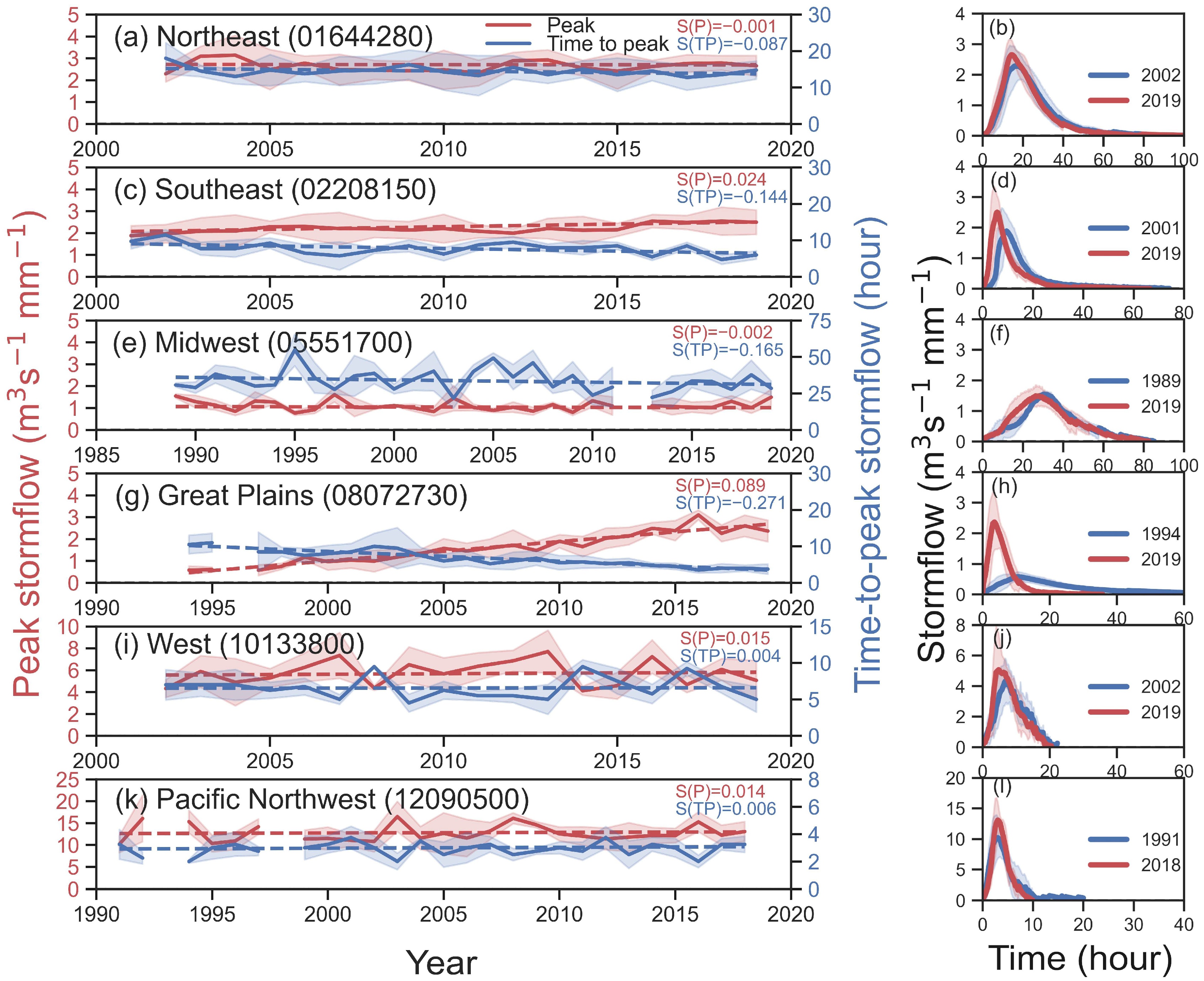
Interannual variation in peak stormflow and time-to-peak stormflow at six watersheds is presented in Figure 3. Upward trends in peak stormflow were observed at four out of six watersheds (Table 2 and Figure 3). On average, the peak stormflows during the study years were 2.64, 2.21, 1.11, 1.60, 5.74, and 12.73 m3 s−1 mm−1 at the Northeast, Southeast, Midwest, Great Plains, West, and Pacific Northwest region watersheds, respectively (results not shown). Based on these peak stormflows, the largest increasing percent change (slope of trend line divided by average peak) in peak stormflow is at the Great Plains watershed, which is 5.54% (Table 2). With this increasing percent change in peak stormflow, the Great Plains watershed expects to increase peak stormflow by 55.4% in the next decade. For this watershed, the urban area increase percentage was also the largest among all watersheds (Table 2). The increasing percent changes of peak stormflow at other watersheds were between 0.11% (1.1% in a decade) at the Pacific Northwest watershed, and 1.10% (11.0% in a decade) at the Southeast watershed. Among six watersheds, two watersheds (Southeast and Great Plains) show significant upward trends in peak stormflow attributed to the significant upward trends in urban areas (Table 2).
Contrary to what was expected, downward peak stormflow trends were observed at two watersheds (Northeast and Midwest regions) with substantial (>9%) increases in urban areas. However, these decreasing peak stormflow percent changes are relatively small, with −0.04% (−0.4% in a decade) at the Northeast watershed and −0.16% (−1.6% in a decade) at the Midwest watershed (Table 2). One of the potential reasons for the decreasing peak stormflows at these watersheds could be the effect of urban stormwater management infrastructures. Such infrastructures are usually smaller (e.g., rain gardens, swales, or retention ponds) for small watersheds and were difficult or even impossible (e.g., pervious pavements, cisterns) to detect in the LCMAP land cover maps with a 30 m spatial resolution. The Northeast region watershed has 1177 stormwater best management practices of 29 different types [31]. Similarly, the Midwest region watershed in Kendall County has a stormwater management plan [32]; however, public data are not available for further details. These stormwater management practices were likely implemented after 2004 when the U.S. Environmental Protection Agency required many cities and counties to integrate such practices, especially green stormwater infrastructure, to obtain compliance with their permit [33,34]. Reduction of peak flows due to stormwater management infrastructures has been reported in urban watersheds [35,36], similar to the observations in this study.
Additionally, the effectiveness of stormwater management may vary based on the types, number, and location/distribution of such infrastructures within a watershed. For example, distributed stormwater infrastructures are more efficient to mitigate runoff volumes and peak flows compared to centralized stormwater management [36]. All six watersheds selected in this study have implemented some forms of stormwater management practices [31,32,37,38,39,40], started as early as the 1990s in the Pacific Northwest region watershed [40]; however, the effectiveness of such practices might not have outweighed the larger effects of increasing urbanization to reflect downward trends in peak stormflows, as observed in the Northeast and Midwest region watersheds. Although this study is unique in using historical observed data (>15 years) as opposed to modeling studies, it did not explore the effects of stormwater management on key stormflow characteristics directly. Previous studies have investigated the effects of stormwater management on several flow characteristics [35,36]. Further studies would benefit from exploring how the flow characteristics vary among watersheds using detailed temporal and distributed information on the types and extent of stormwater management implementations.
Time-to-peak stormflow had a downward trend at four out of six watersheds (Table 2). On average, the time-to-peak stormflows were 14.44, 7.78, 33.76, 6.67, 6.61, and 2.91 h at the Northeast, Southeast, Midwest, Great Plains, West, and Pacific Northwest region watersheds, respectively. The decreasing percent changes of time-to-peak stormflow are relatively higher (−0.49% to −4.06%) at watersheds with a larger urban area increase (>9%) than watersheds with a relatively smaller urban area increase (<6%) with lower increasing percent changes (0.06% to 0.21%) (Table 2). As expected, the largest percent change in time-to-peak stormflow was at the Great Plains watershed at −4.1%, which had the largest increase (20.3%) in the urban area. With this decreasing percent change in time-to-peak stormflow, a 2.71 h faster time-to-peak stormflow is expected in the Great Plains watershed in the next decade (Table 2). The lowest percent change was for the West watershed (0.06%), which had the smallest increase (0.7%) in the urban area. Statistically, a significant downward trend of time-to-peak stormflow was attributed to a significant upward trend in urban areas, only at the Great Plains watershed (Table 2).
3.3. Potential Uncertainties
The results presented are based on annual scale and are not representative of seasonal, monthly, or specific precipitation event-derived changes in stormflow characteristics. The generation of UHs assumes uniform precipitation within a watershed; this assumption may not be valid for all precipitation events that generate stormflows. However, the average UH approach applied is expected to reduce such uncertainties. The observed streamflow data from the USGS are based on the stage–discharge relationship, and this method has an uncertainty of ±6% for ideal conditions [41], and may increase depending on the condition of flow control structure and channel stability [42]. The LCMAP land cover data have a pixel-level overall accuracy above 80% [43], and errors may exist at the pixel level. Potential changes in stormflow characteristics from urban stormwater management infrastructures [7,36] and non-urban areas, such as drainage systems in agricultural croplands [44] or silviculture in forest areas [45], are not quantified. Other static features of watersheds that can affect stormwater characteristics, such as drainage area, length of the longest watercourse, length to center of area, and mainstream slope [46], were considered to have similar effects on two stormflow characteristics during the study years.
3.4. Further Research Direction
Only six watersheds were selected due to the difficulty of finding relatively small (<200 km2) watersheds with long-term 15 min streamflow data and increasing urban area. However, similar studies could be further extended to several watersheds with shorter temporal coverage (<15 years considered in this study) with frequent and severe flooding events. This study captured the overall pattern and trends on two stormflow characteristics at an annual scale based on observed data at the watershed outlets. Further studies can explore sub-watershed scale analysis to identify the location and patterns of land cover changes [47] and compute the relative contribution of sub-watershed areas to stormflows. Additionally, finer-scale studies, such as seasonal, monthly, and event scales can provide better information when needed [18]. Furthermore, additional filters to differentiate the stormflows (e.g., high vs. low flows) could be applied to extend the analysis. Several studies have reported increasing flood risks under growing urbanization [48,49,50], which signifies the increasing importance of similar future studies across flood-prone areas. Upon quantification of altered stormflow characteristics using the UH approach, as applied in this study, the related stakeholders could make watershed-specific decisions in the design and implementation of stormwater management plans and infrastructures.
4. Conclusions
This study investigated the effects of changes in land cover on key stormflow characteristics (peak streamflow and time-to-peak streamflow) of six representative urban watersheds across six broad hydroclimate regions in the conterminous United States. Long-term time series of peak stormflow and time-to-peak stormflow data were generated for the study period varying from 18 to 30 years (1980s to 2010s) at each watershed. The long-term upward trends in peak stormflow and downward trends in time-to-peak stormflow were observed at four out of six watersheds. The watershed in the Great Plains region with the largest percent increase in urban area (20.3%) had the largest increasing percent change in peak stormflow (5.54%) and the largest decreasing percent change in time-to-peak stormflow (−4.06%) among all study watersheds. With this increasing percent change in peak stormflow and decreasing percent change in time-to-peak stormflow, a peak stormflow by 55.4% and 2.71 h faster time-to-peak stormflow is expected in the Great Plains region watershed in the next decade. However, these expected percent changes in the next decade could be affected by legal (urban planning), natural, or physical (e.g., space for expanding urban areas) limits. Two watersheds in the Northeast and Midwest regions had decreasing percent changes in peak stormflow despite increasing urban areas, likely attributed to the implementation of stormwater management practices. This study provided an approach to monitor and quantify the effects of developing urban areas on key stormflow characteristics using the observed streamflow data. Similar studies could be extended to identify watersheds with large changes in stormflow characteristics and for implementing stormwater management practices to minimize future flood risks and associated impacts.
Author Contributions
Conceptualization, G.B.S. and K.K.; methodology, G.B.S. and K.K.; formal analysis, G.B.S. and K.K.; data curation, K.K.; writing—original draft preparation, K.K.; writing—review and editing, G.B.S. and K.K.; visualization, K.K.; supervision, G.B.S.; project administration, G.B.S.; funding acquisition, G.B.S. All authors have read and agreed to the published version of the manuscript.
Funding
This research was funded by the USGS Land Change Science program (contract number: 140G0119C0001).
Institutional Review Board Statement
Not applicable.
Informed Consent Statement
Not applicable.
Data Availability Statement
The data to support the findings of this study are publicly available at https://doi.org/10.5066/P91X5I6L (accessed on 15 June 2022).
Acknowledgments
The authors would like to thank the anonymous reviewers for their constructive comments and suggestions. Any use of trade, firm, or product names is for descriptive purposes only and does not imply endorsement by the U.S. Government.
Conflicts of Interest
The authors declare no conflict of interest.
References
- WMO. Atlas of Mortality and Economic Losses from Weather, Climate and Water Extremes (1970–2019); WMO: Geneva, Switzerland, 2021. [Google Scholar]
- Ward, P.J.; Jongman, B.; Weiland, F.S.; Bouwman, A.; van Beek, R.; Bierkens, M.F.; Ligtvoet, W.; Winsemius, H.C. Assessing flood risk at the global scale: Model setup, results, and sensitivity. Environ. Res. Lett. 2013, 8, 044019. [Google Scholar] [CrossRef]
- IPCC. Managing the Risks of Extreme Events and Disasters to Advance Climate Change Adaptation: Special Report of the Intergovernmental Panel on Climate Change; Field, C.B., Barros, V., Stocker, T.F., Qin, D., Dokken, D.J., Ebi, K.L., Mastrandrea, M.D., Mach, K.J., Plattner, G.-K., Allen, S.K., et al., Eds.; Cambridge University Press: Cambridge, UK, 2012. [Google Scholar]
- Paul, M.J.; Meyer, J.L. Streams in the urban landscape. Annu. Rev. Ecol. Syst. 2001, 32, 333–365. [Google Scholar] [CrossRef]
- Bhaskar, A.S.; Hopkins, K.G.; Smith, B.K.; Stephens, T.A.; Miller, A.J. Hydrologic signals and surprises in US streamflow records during urbanization. Water Resour. Res. 2020, 56, e2019WR027039. [Google Scholar] [CrossRef]
- Tellman, B.; Sullivan, J.; Kuhn, C.; Kettner, A.; Doyle, C.; Brakenridge, G.; Erickson, T.; Slayback, D. Satellite imaging reveals increased proportion of population exposed to floods. Nature 2021, 596, 80–86. [Google Scholar] [CrossRef]
- Loperfido, J.V.; Noe, G.B.; Jarnagin, S.T.; Hogan, D.M. Effects of distributed and centralized stormwater best management practices and land cover on urban stream hydrology at the catchment scale. J. Hydrol. 2014, 519, 2584–2595. [Google Scholar] [CrossRef]
- Cuo, L.; Lettenmaier, D.P.; Alberti, M.; Richey, J.E. Effects of a century of land cover and climate change on the hydrology of the Puget Sound basin. Hydrol. Process. Int. J. 2009, 23, 907–933. [Google Scholar] [CrossRef]
- Hung, C.-L.J.; James, L.A.; Carbone, G.J.; Williams, J.M. Impacts of combined land-use and climate change on streamflow in two nested catchments in the southeastern United States. Ecol. Eng. 2020, 143, 105665. [Google Scholar] [CrossRef]
- Hao, L.; Sun, G.; Liu, Y.; Wan, J.; Qin, M.; Qian, H.; Liu, C.; Zheng, J.; John, R.; Fan, P. Urbanization dramatically altered the water balances of a paddy field-dominated basin in southern China. Hydrol. Earth Syst. Sci. 2015, 19, 3319–3331. [Google Scholar] [CrossRef] [Green Version]
- Shuster, W.D.; Bonta, J.; Thurston, H.; Warnemuende, E.; Smith, D. Impacts of impervious surface on watershed hydrology: A review. Urban Water J. 2005, 2, 263–275. [Google Scholar] [CrossRef]
- Du, J.; Qian, L.; Rui, H.; Zuo, T.; Zheng, D.; Xu, Y.; Xu, C.-Y. Assessing the effects of urbanization on annual runoff and flood events using an integrated hydrological modeling system for Qinhuai River basin, China. J. Hydrol. 2012, 464, 127–139. [Google Scholar] [CrossRef]
- Guan, M.; Sillanpää, N.; Koivusalo, H. Storm runoff response to rainfall pattern, magnitude and urbanization in a developing urban catchment. Hydrol. Process. 2016, 30, 543–557. [Google Scholar] [CrossRef]
- Cheng, S.j.; Wang, R.y. An approach for evaluating the hydrological effects of urbanization and its application. Hydrol. Process. 2002, 16, 1403–1418. [Google Scholar] [CrossRef]
- Sillanpää, N.; Koivusalo, H. Impacts of urban development on runoff event characteristics and unit hydrographs across warm and cold seasons in high latitudes. J. Hydrol. 2015, 521, 328–340. [Google Scholar] [CrossRef]
- Valtanen, M.; Sillanpää, N.; Setälä, H. Effects of land use intensity on stormwater runoff and its temporal occurrence in cold climates. Hydrol. Process. 2014, 28, 2639–2650. [Google Scholar] [CrossRef]
- Todeschini, S. Hydrologic and environmental impacts of imperviousness in an industrial catchment of northern Italy. J. Hydrol. Eng. 2016, 21, 05016013. [Google Scholar] [CrossRef]
- Dougherty, M.; Dymond, R.L.; Grizzard Jr, T.J.; Godrej, A.N.; Zipper, C.E.; Randolph, J. Quantifying long-term hydrologic response in an urbanizing basin. J. Hydrol. Eng. 2007, 12, 33–41. [Google Scholar] [CrossRef] [Green Version]
- Brown, J.F.; Tollerud, H.J.; Barber, C.P.; Zhou, Q.; Dwyer, J.L.; Vogelmann, J.E.; Loveland, T.R.; Woodcock, C.E.; Stehman, S.V.; Zhu, Z. Lessons learned implementing an operational continuous United States national land change monitoring capability: The Land Change Monitoring, Assessment, and Projection (LCMAP) approach. Remote Sens. Environ. 2020, 238, 111356. [Google Scholar] [CrossRef]
- Zhu, Z.; Woodcock, C.E. Continuous change detection and classification of land cover using all available Landsat data. Remote Sens. Environ. 2014, 144, 152–171. [Google Scholar] [CrossRef] [Green Version]
- Jung, I.W.; Chang, H.; Risley, J. Effects of runoff sensitivity and catchment characteristics on regional actual evapotranspiration trends in the conterminous US. Environ. Res. Lett. 2013, 8, 044002. [Google Scholar] [CrossRef] [Green Version]
- USGS. USGS 3D Elevation Program Digital Elevation Model. Available online: https://apps.nationalmap.gov/downloader/ (accessed on 14 October 2021).
- USGS. USGS Water Data of the Nation: U.S. Geological Survey National Water Information System Database. Available online: https://doi.org/10.5066/F7P55KJN (accessed on 23 July 2021).
- USDA. Hydrology Training Series Module 207 Hydrograph Development (NRCS-NEDC-000103). USDA Natural Resources Conservation Services (NRCS) Hydrology Training Series. Available online: https://www.nrcs.usda.gov/wps/portal/nrcs/detail/national/nedc/?cid=stelprdb1047203 (accessed on 7 December 2021).
- Croke, B. A technique for deriving an average event unit hydrograph from streamflow—only data for ephemeral quick-flow-dominant catchments. Adv. Water Resour. 2006, 29, 493–502. [Google Scholar] [CrossRef]
- Hewlett, J.D.; Hibbert, A.R. Factors Affecting the Response of Small Watersheds to Precipitation in Humid Areas; Sopper, W.E., Lull, H.W., Eds.; Elsevier: New York, NY, USA, 1967; pp. 275–290. [Google Scholar] [CrossRef]
- Terink, W. A Python Package for Separation of Flow Time-Series into Peak Flow and Basefloe, version 1.0.1; 2019. Available online: https://hydrograph-py.readthedocs.io/en/latest/index.html (accessed on 15 June 2022).
- Lana-Renault, N.; Latron, J.; Karssenberg, D.; Serrano-Muela, P.; Regüés, D.; Bierkens, M. Differences in stream flow in relation to changes in land cover: A comparative study in two sub-Mediterranean mountain catchments. J. Hydrol. 2011, 411, 366–378. [Google Scholar] [CrossRef] [Green Version]
- Latron, J.; Soler, M.; Llorens, P.; Gallart, F. Spatial and temporal variability of the hydrological response in a small Mediterranean research catchment (Vallcebre, Eastern Pyrenees). Hydrol. Process. Int. J. 2008, 22, 775–787. [Google Scholar] [CrossRef]
- Khand, K.B.; Senay, G.B. Unit Hydrographs of Evolving Urban Watersheds across the United States: U.S.; Geological Survey Data Release: Reston, VA, USA, 2022; Available online: https://doi.org/10.5066/P91X5I6L (accessed on 15 June 2022). [CrossRef]
- Loudoun-County. Loudoun County GeoHub Portal. Available online: https://geohub-loudoungis.opendata.arcgis.com/ (accessed on 23 March 2022).
- Kendall-County. Kendall Countywide Stormwater Management Ordinance. Available online: https://www.kendallcountyil.gov/departments/planning-building-zoning/planning-and-zoning-application-forms-ordinances (accessed on 23 March 2022).
- Spahr, K.M.; Bell, C.D.; McCray, J.E.; Hogue, T.S. Greening up stormwater infrastructure: Measuring vegetation to establish context and promote cobenefits in a diverse set of US cities. Urban For. Urban Green. 2020, 48, 126548. [Google Scholar] [CrossRef]
- USEPA. Green Infrastructure: Enforcement. Available online: https://www.epa.gov/green-infrastructure/enforcement (accessed on 12 April 2021).
- Conley, G.; McDonald, R.I.; Nodine, T.; Chapman, T.; Holland, C.; Hawkins, C.; Beck, N. Assessing the influence of urban greenness and green stormwater infrastructure on hydrology from satellite remote sensing. Sci. Total Environ. 2022, 817, 152723. [Google Scholar] [CrossRef]
- Hopkins, K.G.; Woznicki, S.A.; Williams, B.M.; Stillwell, C.C.; Naibert, E.; Metes, M.J.; Jones, D.K.; Hogan, D.M.; Hall, N.C.; Fanelli, R.M. Lessons learned from 20 y of monitoring suburban development with distributed stormwater management in Clarksburg, Maryland, USA. Freshw. Sci. 2022, 41. [Google Scholar] [CrossRef]
- Gwinnett-County. Gwinnett County BMPs and Detention Ponds. Available online: https://www.gwinnettcounty.com/web/gwinnett/departments/water/whatwedo/stormwater/bmpsanddetentionponds (accessed on 7 June 2022).
- Harris-County. Harris County Flood Control District. Available online: https://www.hcfcd.org/ (accessed on 9 June 2022).
- Summit-County. Summit County STORM WATER. Available online: https://summitcounty.org/755/Storm-WaterMS4 (accessed on 7 June 2022).
- Pierce-County. Pierce County (Managing Stormwater Runoff). Available online: https://www.piercecountywa.gov/1855/Managing-Stormwater-Runoff (accessed on 7 June 2022).
- Boning, C. Policy Statement on Stage Accuracy. Technical Memorandum No. 93-07; USGS: Washington, DC, USA, 1992.
- Harmel, R.; Cooper, R.; Slade, R.; Haney, R.; Arnold, J. Cumulative uncertainty in measured streamflow and water quality data for small watersheds. Trans. ASABE 2006, 49, 689–701. [Google Scholar] [CrossRef]
- Stehman, S.V.; Pengra, B.W.; Horton, J.A.; Wellington, D.F. Validation of the US Geological Survey’s Land Change Monitoring, Assessment and Projection (LCMAP) Collection 1.0 annual land cover products 1985–2017. Remote Sens. Environ. 2021, 265, 112646. [Google Scholar] [CrossRef]
- Schilling, K.E.; Helmers, M. Effects of subsurface drainage tiles on streamflow in Iowa agricultural watersheds: Exploratory hydrograph analysis. Hydrol. Process. 2008, 22, 4497–4506. [Google Scholar] [CrossRef]
- Swank, W.T.; Swift, J.L.; Douglass, J. Streamflow Changes Associated with Forest Cutting, Species Conversions, and Natural Disturbances. In Forest Hydrology and Ecology at Coweeta; Springer: New York, NY, USA, 1988; pp. 297–312. [Google Scholar] [CrossRef]
- Taylor, A.B.; Schwarz, H.E. Unit-hydrograph lag and peak flow related to basin characteristics. Eos Trans. Am. Geophys. Union 1952, 33, 235–246. [Google Scholar] [CrossRef]
- Debbage, N.; Shepherd, J. The influence of urban development patterns on streamflow characteristics in the Charlanta Megaregion. Water Resour. Res. 2018, 54, 3728–3747. [Google Scholar] [CrossRef]
- Avashia, V.; Garg, A. Implications of land use transitions and climate change on local flooding in urban areas: An assessment of 42 Indian cities. Land Use Policy 2020, 95, 104571. [Google Scholar] [CrossRef]
- O’Donnell, E.C.; Thorne, C.R. Drivers of future urban flood risk. Philos. Trans. R. Soc. A 2020, 378, 20190216. [Google Scholar] [CrossRef] [PubMed] [Green Version]
- Hemmati, M.; Ellingwood, B.R.; Mahmoud, H.N. The role of urban growth in resilience of communities under flood risk. Earth Future 2020, 8, e2019EF001382. [Google Scholar] [CrossRef] [Green Version]
Figure 1.
Locations of six representative study watersheds (a) with land cover maps and urban area for 2019 with urban area percent (D) for start/end study years across six broad hydroclimate regions of the conterminous United States (b–g). The green stars (b–g) represent the outlets of the watersheds. Land cover data sourced from the Land Change Monitoring, Assessment, and Projection (LCMAP) Collection 1.1 (https://www.usgs.gov/core-science-systems/eros/lcmap, accessed on 15 June 2022).

Figure 2.
Land cover data of six watersheds from 1985 to 2019. The black dashed line shows the study years and corresponding stormflow data, and ΔD indicates the increase in urban area percentage at each watershed. Data sourced from the Land Change Monitoring, Assessment, and Projection (LCMAP) Collection 1.1 (https://www.usgs.gov/core-science-systems/eros/lcmap, accessed on 15 June 2022).

Figure 3.
The first panel (a,c,e,g,i,k) shows the peak stormflow (red solid line) and time-to-peak stormflow (blue solid line) during the study years at six watersheds. The second panel (b,d,f,h,j,l) shows the average unit hydrographs for the start and end study years of the corresponding watersheds in the first panel (for example, the sub-figure (b) corresponds to the sub-figure (a) for the Northwest region watershed). The shaded area in both panel sub-figures is the standard deviation. The S(P) and S(TP) in the first panel are the slopes of trend lines of peak stormflow (red dashed line) and time-to-peak stormflow (blue dashed line), respectively. A few years of data are missing for three watersheds (e,g,k) due to limited streamflow data and/or due to limited stormflow events to generate unit hydrographs.


Table 1.
Summary of study watersheds including the U.S. Geological Survey (USGS) streamgage information, watershed area, and study years.
Table 1.
Summary of study watersheds including the U.S. Geological Survey (USGS) streamgage information, watershed area, and study years.
| Region | USGS Streamgage Site Number [23] | Site Name | State (County) | Watershed Area, km2 | Study Years |
|---|---|---|---|---|---|
| Northeast | 01644280 | Broad Run near Leesburg, VA | Virginia (Loudoun) | 197.6 | 2002–2019 |
| Southeast | 02208150 | Alcovy River at New Hope Road, near Grayson, GA | Georgia (Gwinnett) | 80.0 | 2001–2019 |
| Midwest | 05551700 | Blackberry Creek near Yorkville, IL | Illinois (Kendall) | 167.1 | 1989–2019 |
| Great Plains | 08072730 | Bear Creek near Barker, TX | Texas
(Harris) | 54.5 | 1994–2019 |
| West | 10133800 | East Canyon Creek near Jeremy Ranch, UT | Utah
(Summit) | 151.4 | 2002–2019 |
| Pacific Northwest | 12090500 | Clover Creek near Tillicum, WA | Washington (Pierce) | 164.1 | 1991–2018 |
Table 2.
Trends in peak stormflow, time-to-peak stormflow, and urban (developed) area. Upward or downward trends are based on the positive or negative slopes of trend lines, respectively. The annual percent change of increase (positive values) or decrease (negative values) in peak stormflow (second column) and time-to-peak stormflow (third column) at each watershed is computed as a ratio of slopes of trend lines divided by their respective average values during the study years. The annual percent change in peak stormflow was multiplied by 10 to obtain the expected decadal percent change in peak stormflow (second column). The slopes of trend lines of time-to-peak stormflow were multiplied by 10 to compute expected changes in decadal time-to-peak stormflow (third column).
| Region (Site Number) | Peak Stormflow (Annual Percent Change, Decadal Percent Change) | Time-to-Peak Stormflow (Annual Percent Change, Decadal Change in Hour) | Number of Selected Event Scale Unit Hydrographs | Urban (Developed) Area + |
|---|---|---|---|---|
| Northeast (01644280) | Downward (−0.04, −0.4) | Downward (−0.60, −0.87) | 235 | upward * |
| Southeast (02208150) | upward * (1.10, 11.0) | Downward (−1.85, −1.44) | 189 | upward * |
| Midwest (05551700) | downward
(−0.16, −1.6) | Downward (−0.49, −1.65) | 168 | upward * |
| Great Plains (08072730) | upward *
(5.54, 55.4) | downward * (−4.06, −2.71) | 297 | upward * |
| West (10133800) | upward
(0.26, 2.6) | Upward (0.06, 0.04) | 162 | upward * |
| Pacific Northwest (12090500) | upward
(0.11, 1.1) | Upward (0.21, 0.06) | 201 | upward * |
Note(s): * Statistically significant (p-value ≤ 0.05). + Land cover data were obtained from the Land Change Monitoring, Assessment, and Projection (LCMAP) Collection 1.1 (https://www.usgs.gov/core-science-systems/eros/lcmap, accessed on 15 June 2022).
Publisher’s Note: MDPI stays neutral with regard to jurisdictional claims in published maps and institutional affiliations. |
© 2022 by the authors. Licensee MDPI, Basel, Switzerland. This article is an open access article distributed under the terms and conditions of the Creative Commons Attribution (CC BY) license (https://creativecommons.org/licenses/by/4.0/).
Share and Cite
MDPI and ACS Style
Khand, K.; Senay, G.B. Land Cover Change Effects on Stormflow Characteristics across Broad Hydroclimate Representative Urban Watersheds in the United States. Water 2022, 14, 2256. https://doi.org/10.3390/w14142256
AMA Style
Khand K, Senay GB. Land Cover Change Effects on Stormflow Characteristics across Broad Hydroclimate Representative Urban Watersheds in the United States. Water. 2022; 14(14):2256. https://doi.org/10.3390/w14142256
Chicago/Turabian StyleKhand, Kul, and Gabriel B. Senay. 2022. "Land Cover Change Effects on Stormflow Characteristics across Broad Hydroclimate Representative Urban Watersheds in the United States" Water 14, no. 14: 2256. https://doi.org/10.3390/w14142256
Note that from the first issue of 2016, this journal uses article numbers instead of page numbers. See further details here.