Trends and Climate Elasticity of Streamflow in South-Eastern Brazil Basins

Abstract

Trends in streamflow, rainfall and potential evapotranspiration (PET) time series, from 1970 to 2017, were assessed for five important hydrological basins in Southeastern Brazil. The concept of elasticity was also used to assess the streamflow sensitivity to changes in climate variables, for annual data and 5-, 10- and 20-year moving averages. Significant negative trends in streamflow and rainfall and significant increasing trend in PET were detected. For annual analysis, elasticity revealed that 1% decrease in rainfall resulted in 1.21–2.19% decrease in streamflow, while 1% increase in PET induced different reductions percentages in streamflow, ranging from 2.45% to 9.67%. When both PET and rainfall were computed to calculate the elasticity, results were positive for some basins. Elasticity analysis considering 20-year moving averages revealed that impacts on the streamflow were cumulative: 1% decrease in rainfall resulted in 1.83–4.75% decrease in streamflow, while 1% increase in PET induced 3.47–28.3% decrease in streamflow. This different temporal response may be associated with the hydrological memory of the basins. Streamflow appears to be more sensitive in less rainy basins. This study provides useful information to support strategic government decisions, especially when the security of water resources and drought mitigation are considered in face of climate change.

1. Introduction

A number of studies have reported streamflow reduction in several important basins throughout the world [1,2,3,4,5], putting enormous social, environmental and economic pressure on the world’s population and leading to great insecurity when it comes to water, energy and food supply [6,7]. This phenomenon can be associated with the increase on frequency and intensity of extreme climatic events, such as heat waves and droughts [8], as well anthropogenic interferences in the climate via greenhouse gases emission and land use and cover modifications [9,10,11]. Both interferences together affect streamflow discharge and water resources management. In relation to climate variations, streamflow response is modified through changes in the precipitation regime and evaporation. To quantify these modifications is of considerable importance for a better understanding and planning of adaptation strategies when it comes to climate change, drought management and water security plans.

The same deficit in rainfall may not induce the same impacts on hydrological processes, as soil, vegetation, land use, and basin’s characteristics vary from region to region; therefore, streamflow respond differently to the same climate variations. A method of measuring and comparing these impacts on drainage basins of different regions is the climate elasticity of streamflow. This concept was firstly introduced to assess the sensitivity of the streamflow to the modifications in some climatic variables [12]. Elasticity is a lumped representation of the hydrological effects of a multitude of processes affecting the response of streamflow to variations in climate variables [13]. Elasticity estimators provide a measure of the streamflow resilience to changes in meteorological variables, such as rainfall and potential evapotranspiration [14,15], being particularly useful as initial estimates of climate change [16,17]. Elasticity can also be understood as the percent change of streamflow resulting from a 1% change in precipitation or other climate variables.

Regarding streamflow elasticity to precipitation, numerous studies have indeed identified these controls for basins ranging from 50 (or smaller) to 76,000 km² of drainage area in various regions worldwide, such as Australia [18], China [16], USA [14], Korea [17], Brazil [19], France [20] and Bulgaria [21]. In Australia, streamflow elasticity varying from 2.0 and 3.5 in 70% of the 219 watersheds of various drainage area were reported [22]. Indeed, in Southwestern Australia, the average contribution of climate and vegetation to streamflow elasticity is almost equal, whilst climate change also has an indirect effect in being able to change catchment characteristics (vegetation structure as well as soil water storage) [23]. In Brazil, elasticity values ranging from 0.54 to 9.79 in projected impacts of climate change on the streamflow of large Brazilian basins were reported in [24]. The lowest values were found in the Amazon and central–western areas of the country, whilst Northeastern Brazil exhibited the highest values.

Elasticity can be obtained using as basis hydroclimatic variables and non-parametric estimators (empirical estimators) or rainfall-runoff models (theoretical estimators). The empirical (data-based rather than model-based) estimation of the elasticity of streamflow is not constrained by the assumptions of modelling or requires model validation [14,20,25], and some studies have even found out great similarities between modelling and the nonparametric method [22,26]. Streamflow elasticity is usually calculated with annual data; however, [20] reported that to analyse sub-periods of 20 years provides a better performance compared to the other durations, especially considering elasticity to potential evapotranspiration. In relation to data length, although long time series are adequate to compute the climatic impact on streamflow, 20-year data length is the minimum suggested [20]. Shorter data length causes large variability because soil water storage can be neglected [14] whereas the long data length is not easily obtained [27].

In Southeastern Brazil (SEB), total rainfall has decreased in recent decades [6], being accompanied by increasing air temperatures [28] and consequently increasing frequency of hydrological droughts [29,30]. Major droughts occurred in SEB in 1953/54, 1962/63, 1970/71, 2001 and 2014/15. Despite a complex subject of study, drought events have always been characterized by rainfall deficits during the summer and the weak South Atlantic Convergence Zone (SACZ) activity, as SACZ is the most important convective system that brings precipitation to SEB during austral summer periods [31]. Studies show that temperature and rainfall extremes have been increasing in SEB during the recent decades [32,33]. These phenomena caused an unbalance of the water cycle, affecting streamflow, reducing inflow, and therefore leading to water insecurity.

Prolonged droughts in Southeast Brazil mostly originate in the Indian Ocean (eastern Africa, western Australia and southern Asia) [8,34]. The formation of intense precipitation over the Indian Ocean generates disturbances in the atmosphere that propagate eastward and reach South America, contributing to the formation of a large mass of dry and hot air, which prevents the formation of rain over Southeast Brazil. In addition, this dry air mass blocks the entry of water vapor mass originating in the Amazon. Besides, according to the authors, dry and hot summers in the Southeast have been occurring more frequently and intensely in the last 20 years, which may be related to the trend of increasing frequency, intensity, duration, and extent of marine heat waves [8].

The hydrological droughts in 2001 and 2014/15 in SEB were the most challenging for human activities and induced different impacts on the streamflow of the region. In 2001, SEB experienced an unprecedented energy crisis due to water shortage for hydropower generation in almost all reservoirs basins [35]. In 2014/15, the consequences were disastrous mainly for water supply and hydropower generation [6,7]. In the Cantareira System, one of the most important water supply system of the Metropolitan Region of São Paulo City (MRSP), the streamflow decreased dramatically [31], affecting more than 8.8 million people and leading to the exceptional consumption of pumped water in 2014 and 2015 [36]. In the Três Marias reservoir, located upstream of the São Francisco River in the State of Minas Gerais, streamflow was well below the Long-Term Mean (LTM), causing the drastic lowering of water level in the reservoir. In 2014, annual streamflow represented 28% of the LTM and the reservoir reached 2.6% in November of that year, its lowest level since the beginning of its operation [29].

Due to the frequent droughts observed in the last years/decades and the different impacts observed in the streamflow, this paper aims to characterize the historical evolution of the hydroclimatic parameters in SEB during the last five decades. Therefore, the objectives of this paper are: (1) to identify trends and abrupt changes in the historical series of streamflow, rainfall and potential evapotranspiration; (2) to assess the climate elasticity of streamflow, and (3) to identify the most sensitive SEB basin(s) to extremes of climate variability.

2. Materials and Methods

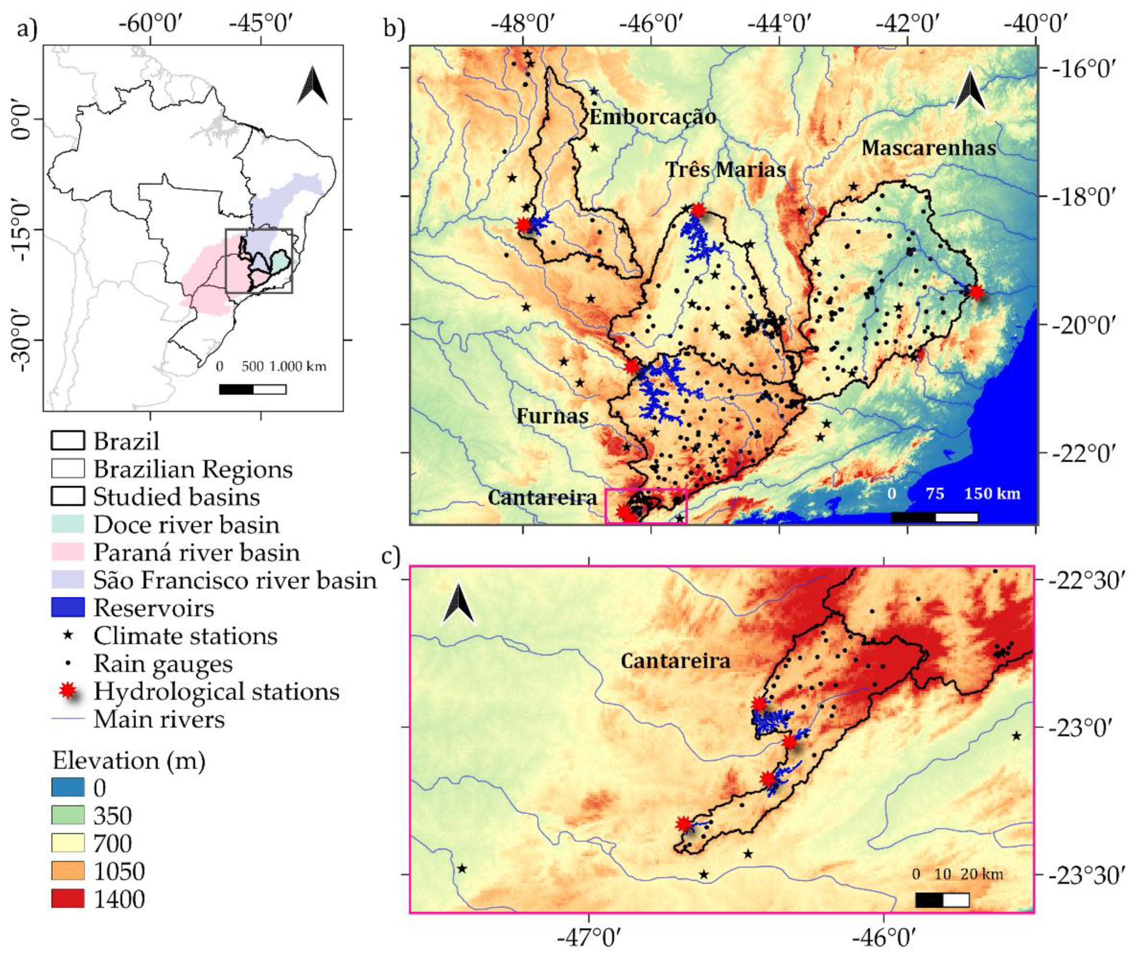
2.1. Study Area

In this paper, we assessed five major drainage basins located in SEB, important for multisectoral water use and management: The Cantareira system—for supplying water for the largest metropolitan region of South America, and the drainage basins of the reservoirs Furnas, Emborcação, Três Marias and Mascarenhas de Moraes—for hydropower generation to SEB (Figure 1). This region includes great cities such as São Paulo, Rio de Janeiro and Belo Horizonte, and holds 41.9% of the Brazilian population, equivalent to about 80 million inhabitants [37]. In addition, this region is home to the largest industrial axis of South America, contributing to 55.3% of the National Gross Domestic Product [38]. Moreover, SEB together with the Central-Western Brazil, is responsible for approximately 70% of the hydropower generation capacity of the country [39], representing the main source of energy in Brazil. This high population concentration in SEB and economic significance emphasise the importance of water resources, demanding large concentration of reservoirs.

The Emborcação drainage basin (~29,000 km²) is located in the Paranaíba River basin, and the Furnas drainage basin (~51,000 km²), in the Rio Grande River basin. Both rivers are tributaries of the Paraná River, one of the most exploited rivers for the hydropower generation in Brazil. The Três Marias drainage basin (~51,000 km²), besides hydropower generation, is also managed for water supply and irrigation, and is located upstream of the São Francisco River. The São Francisco River, whose headwater is located in SEB, is important for Northeastern Brazil because is the largest perennial river in the region. The Mascarenhas drainage basin (~72,000 km²) is located in the Doce River. This river was largely contaminated due to mining dam collapse in 2015 [40]. The Cantareira System (~2300 km²) is a set of reservoirs, affected by water shortage between 2014 and 2016 [31,34]. Detailed description of these basins, such as information about soil, land use coverage and PIB can be found in Appendix A 

Table A1. Summary description of studied basins.

		Emborcação	Três Marias	Mascarenhas	Furnas	Cantareira
Area [km2]		29,057	51,044	71,573	51,687	2280
Census 2010	Population	444,279	2,776,565	2,906,492	2,467,657	204,815
	PIB	9,284,611	57,824,702	33,261,946	29,283,999	3,920,477
Climate		Aw: 99%	Aw: 64%	Aw: 59%	Cwa:77%	Cwb: 54%
Solo [% of area]	Oxisols	43	36	60	55	71
	Inceptisols	39	44	3	34	0
	Ultisols	8	17	35	8	29
	Entisols	5	0	2	0	0
	Water	1	3	0	3	0
	Others	4	0	0	0	0
Land-use type [% of area]	Pasture	43	41	34	37	4
	Livestock and agriculture	19	25	28	32	15
	Forest	6	13	24	8	33
	Crop	16	3	4	8	0
	Urban	1	3	2	3	44
	Others	15	15	8	12	4

Note: PIB (1 R$~0.569 USD; 2010 values).

.

SEB is inserted in three climatic zones: tropical savannah (Aw), temperate with dry winter and warm summer (Cwb), and temperate with dry winter and hot summer (Cwa) [41]. All of them are characterized by six rainy months during the austral summer (October to March, with maximum precipitations in December–February), followed by six dry months during the austral winter (April to September). Annual rainfall (P), potential evapotranspiration (PET) and streamflow (Q) values for each watershed are listed in

Table 1. Hydrological characterization of the studied watershed (1970–2017): annual averages of rainfall (P), potential evapotranspiration (PET), streamflow (Q), runoff index (Q/P) and aridity index (PET/P).

Basin	Annual P (mm)	Annual PET (mm)	Annual Q (mm)	Runoff Index (Q/P)	Aridity Index (PET/P)
Furnas	1471	1533	544	0.37	1.04
Emborcação	1482	1618	497	0.34	1.09
Mascarenhas	1233	1535	384	0.31	1.25
Três Marias	1392	1610	405	0.29	1.16
Cantareira	1562	1424	579	0.37	0.91

. Annual P varies from 1233 to 1562 mm, PET varies from 1424 to 1618 mm, while Q varies from 384 to 579 mm. Runoff index (Q/P) varies between 0.29 in Três Marias, and 0.37 in Cantareira and in Furnas. Aridity index (PET/P) varies between 0.91 in Cantareira system and 1.25 in Mascarenhas.

2.2. Data Collection

2.2.1. Rainfall Data

Rainfall (P) data were obtained from automatic and conventional stations from: (i) the National Institute of Meteorology (INMET—http://www.inmet.gov.br/portal/ (accessed on 25 November 2020)), and (ii) the National Water Agency (ANA—http://www.snirh.gov.br/hidroweb/publico/ (accessed on 25 November 2020)) for the period 1970–2017. For the Cantareira system, precipitation data were also obtained from the Water and Electricity Department of the State of Sao Paulo (DAEE) for the period 1970–2017. The distribution of the rain gauge is shown in Figure 1. Daily precipitation data were estimated from the arithmetic mean of the available station data for each basin.

2.2.2. Streamflow Data

Streamflow (Q) dataset were obtained from the National Electric System Operator (ONS—http://www.ons.org.br/ (accessed on 25 November 2020)) and from the water and waste management company of the State of São Paulo—(SABESP—http://mananciais.sabesp.com.br/Home (accessed on 25 November 2020)), the latter regarding the Cantareira system. For this system, streamflow represents the sum of the four interconnected reservoirs (Figure 1c). Data from ONS refer to the naturalized flow estimated by water balance. Naturalized flow is defined as the hypothetical flow observed in the absence of human activities in the basin upstream of the gauge station [42]. In this case, ONS estimated the natural flow without the impacts of dams, weirs, extraction and river management. The Cantareira system has a small headwater, and so there is no significant regulation in upstream basin.

2.2.3. Potential Evapotranspiration Data

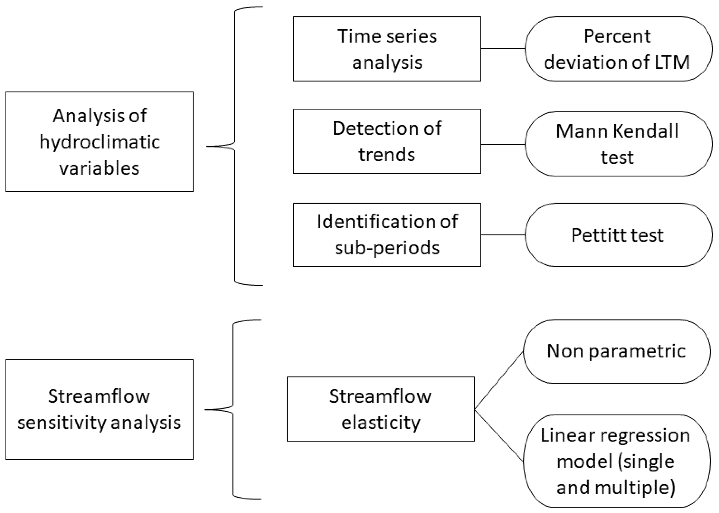
Daily potential evapotranspiration (PET) was estimated by the Hargreavess–Samani (HS) method, a semiempirical approximation that incorporates extraterrestrial radiation in combination with temperature, as indicators of global radiation, and the daily temperature range, as an indicator of humidity and cloudiness [43]. Daily maximum and minimum 2-m air temperature was obtained from the climatological stations of INMET for the 1970–2017 period (Figure 1). Although other methods such as weighting for elevation or Thiessen polygons can be better alternatives, the arithmetic mean was used for its simplicity. For 22 weather stations over Sao Paulo State, [44], eight empirical evapotranspiration estimation methods were compared, including the HS. The results showed that the HS method is an alternative for PET calculation (R² = 0.87), which only requires measuring Tmax, Tmin, and T. In addition, other studies considering data from weather stations inserted in other parts of the study area, including Minas Gerais State also showed that the HS method is efficient and satisfactory for estimating PET [45,46].

2.3. Data Analysis

Figure 2 is a flow chart the steps followed in the study, as well as the analysis carried out in each step and methods applied in the analysis.

2.3.1. Time-Series Analysis

In order to analyse the climatic variability in the selected basins, historical anomaly time series for P, PET and Q were calculated using percent deviation of long-term mean (SXI), as described in Equation (1):

$$SXI=\left(X_t-\overline{X}\right)/\overline{X},$$

(1)

where, $X_t$ refers to P, PET or Q computed for each time scale (temporal aggregation interval) and $\overline{X}$ refers to long-term mean of these variables. Annual means and 5-, 10- and 20-year moving averages of P, PET and Q were used to compute the time series. The long-term mean was obtained from the data available for each time scale. For the analysis of moving averages, the central year is used to represent the period. Time series analysis enables the determination of the dry and wet years/periods in the record.

2.3.2. Trend Analysis

The non-parametric Mann-Kendall test (MK) was applied to hydroclimatic time series to test any increasing or decreasing trend [47]. It has been widely used in previous streamflow trend analyses [2,3,5,48,49,50]. The MK test is a nonparametric approach that makes no assumption about data distribution (such as normal distribution), being robust in both considering outliers and nonlinear trends. This test consists of comparing each value of the time-series with the remaining ones, always in sequential order. If $X_1$; $X_2$; $X_3$; …; $X_n$ is the time series of length $n$, then the Mann–Kendall statistic S is given by [51,52,53,54]:

$$S={\displaystyle \sum }_{i=1}^{n-1} {\displaystyle \sum }_{j=i+1}^n \mathrm{sign}\left(X_j- X_i\right) ,$$

(2)

where,

$$\mathrm{sign} \left(X_j- X_i\right)=\left\{\begin{array}{c}1 f\mathrm{or} \left(X_j- X_i\right)>0\\ 0 f\mathrm{or} \left(X_j- X_i\right)=0\\ -1 \mathrm{or} \left(X_j- X_i\right)<0\end{array}\right. ,$$

(3)

The MK statistic Z is given by:

$$\mathrm{Z}=\left\{\begin{array}{c}\frac{S-1}{\sqrt{V \left(S\right)}} f\mathrm{or} S>0\\ 0 f\mathrm{or} S=0\\ \frac{S+1}{\sqrt{V \left(S\right)}} \mathrm{or} S<0\end{array}\right. ,$$

(4)

where,

$$\mathrm{V}\left(S\right)=\frac{n\left(n-1\right)\left(2n+S\right)}{18} ,$$

(5)

A positive (negative) Z value indicates an increasing (decreasing) trend [55]. The null hypothesis in the MK test is that the data are independent and randomly ordered. In this paper the null hypothesis was rejected at p-value < 0.05 (significance level was 5%).

2.3.3. Break Point (Homogeneity) Analysis

The non-parametric Pettitt test, a method for testing time series homogeneity used in a number of hydro-climatological studies [56], was applied in order to detect ruptures in the hydroclimatic time series, i.e., the existence of different sub-periods. Pettitt’s test is a rank-based nonparametric statistical test similar to the Mann–Whitney test [57]. The test identifies significant break points and was used to assess the null hypothesis—when the data are homogeneous, i.e., there is no change in the mean value of each period. Pettitt’s tests verify whether two samples X₁, … X_t and X_t+1, …, X_T are from the same population. Letting t be the time in a time series, the Pettitt test index (U_t,T) is defined as follows:

$$U_{t,T}={\displaystyle \sum }_{i=1}^t {\displaystyle \sum }_{j=t+1}^T \mathrm{sign}\left(X_j- X_i\right) , 1\le t\le T$$

(6)

where,

$$\mathrm{sign} \left(X_j- X_i\right)=\left\{\begin{array}{c}1 f\mathrm{or} \left(X_j- X_i\right)>0\\ 0 f\mathrm{or} \left(X_j- X_i\right)=0\\ -1 \mathrm{or} \left(X_j- X_i\right)<0\end{array}\right. ,$$

(7)

where $t$ is the change point, T is the time series length. The statistical K_t determines the time at which U_t,T has the greatest absolute value [58]. This test locates the point at which the abrupt change occurs (break) in a time series and calculates the level of statistical significance without prior knowledge of the point in time where it occurs. The probability of significance is approximated by the following equation:

$$P \cong 2 \exp \left(\frac{-6K_t{}^2}{\left(T^3+T^2\right)}\right)$$

(8)

If p-value < 0.05, the null hypothesis can be rejected and therefore a significant break point be identified, i.e., there is a date at which there is a change in the data trend.

Based on the results of the Pettitt test, the time series were divided into sub-periods, using the year of the break point as an inflection. Results of the Pettitt test are expressed as the year of the break point. For moving average analysis, the break point is expressed as the central year of the period. To assess the changes between the two sub-periods, pre- and post-break point, the ratio of change (∆), which quantifies the deviation of the mean value of each variable after the break point, was obtained using Equation (2):

$$\Delta =\frac{X_{post}-X_{pre}}{X_{pre}}\times 100,$$

(9)

where $X_{post}$ and $X_{pre}$ are the mean values of the post- and pre-break points.

2.3.4. Elasticity Methods

The elasticity of streamflow (ε) may be defined as the sensitivity of hydrological systems to the long-term climate fluctuations and can be understood as the proportional change in streamflow to the change in some climatological variable, such as P or PET. Thus, ε is defined as:

$$\epsilon \left(X,Q\right)=\left(\frac{dQ/Q}{dX/X}\right)=\left(\frac{dQ}{dX} \frac{X}{Q}\right),$$

(10)

where $Q$ refers to streamflow and $X$ refers to P or PET. In this paper ε was estimated using two empirical (based on the observed dataset) estimators: a nonparametric and a statistical approach. The nonparametric estimator of elasticity (NP) computes the impacts of anomalies of a single climatological parameter on the streamflow anomalies without assumptions of data distribution, as proposed by [14] and applied in several studies (e.g., [13]). It is calculated using Equation (4):

$$\epsilon =median\left(\frac{Q_t-\overline{Q}}{X_t-\overline{X}} \frac{\overline{X}}{\overline{Q}}\right),$$

(11)

where $Q_t$ refers to streamflow and $X_t$ refer to P or PET, respectively computed for each aggregation time, from one year to multiple years;$\overline{Q}$ refers to mean Q and $\overline{X}$ refers to mean P or PET.

Linear regression is a method of establishing the statistical relationship between a response, or dependent, variable on one or more explanatory, or independent, variables. One way of finding the parameters of the regression model is finding the intercept and coefficient pairs (the parameters of the model) that minimizes the residual sum of squares of the estimated values. This solution is known as ordinary least squares (OLS). It is a versatile method that can include metric and non-metric variables, and one (simple linear regression) or several (multiple linear regression) independent variables (or predictors). We applied two single linear regressions having either P or PET as independent variables (Equations (12) and (13), hereafter termed as OLS-1), and a multiple linear regression having both P and PET as independent variables (Equation (14), hereafter termed as OLS-2). In the second case, each coefficient provides a partial association between dependent and independent variables, after statistically controlling for other variables [59]. The equations of the linear regressions are:

$$\Delta Q=\mathsf{\alpha }+\epsilon p\ast \Delta P,$$

(12)

$$\Delta Q=\mathsf{\alpha }+\epsilon pet\ast \Delta PET,$$

(13)

$$\Delta Q=\mathsf{\alpha }+\epsilon p\ast \Delta P+\epsilon pet\ast \Delta PET,$$

(14)

where $\Delta X$ refers to the percent change of Q, P or PET respectively (e.g., $\Delta Q=\left(Q-\overline{Q}\right)/\overline{Q}$).

If ε is greater than 1, a 1% anomaly in a climate variable would result in a streamflow anomaly greater than 1%. An ε value of 3 indicates that a 1% increase in rainfall, for example, would lead to 3% increase in streamflow.

Streamflow elasticity is usually calculated with annual data. However, some studies revealed that elasticity depends on the aggregation time scale, i.e., the duration of the sub-periods can affect the performance of the elasticity estimator, mainly considering the regression model method [13]. It is suggested to use decadal elasticities instead of annual elasticities in climate impact analyses in order to account for their scaling behaviour [20]. In this paper, annual and 5-, 10- and 20-year moving averages of hydroclimate variables were used to calculate ε.

3. Results

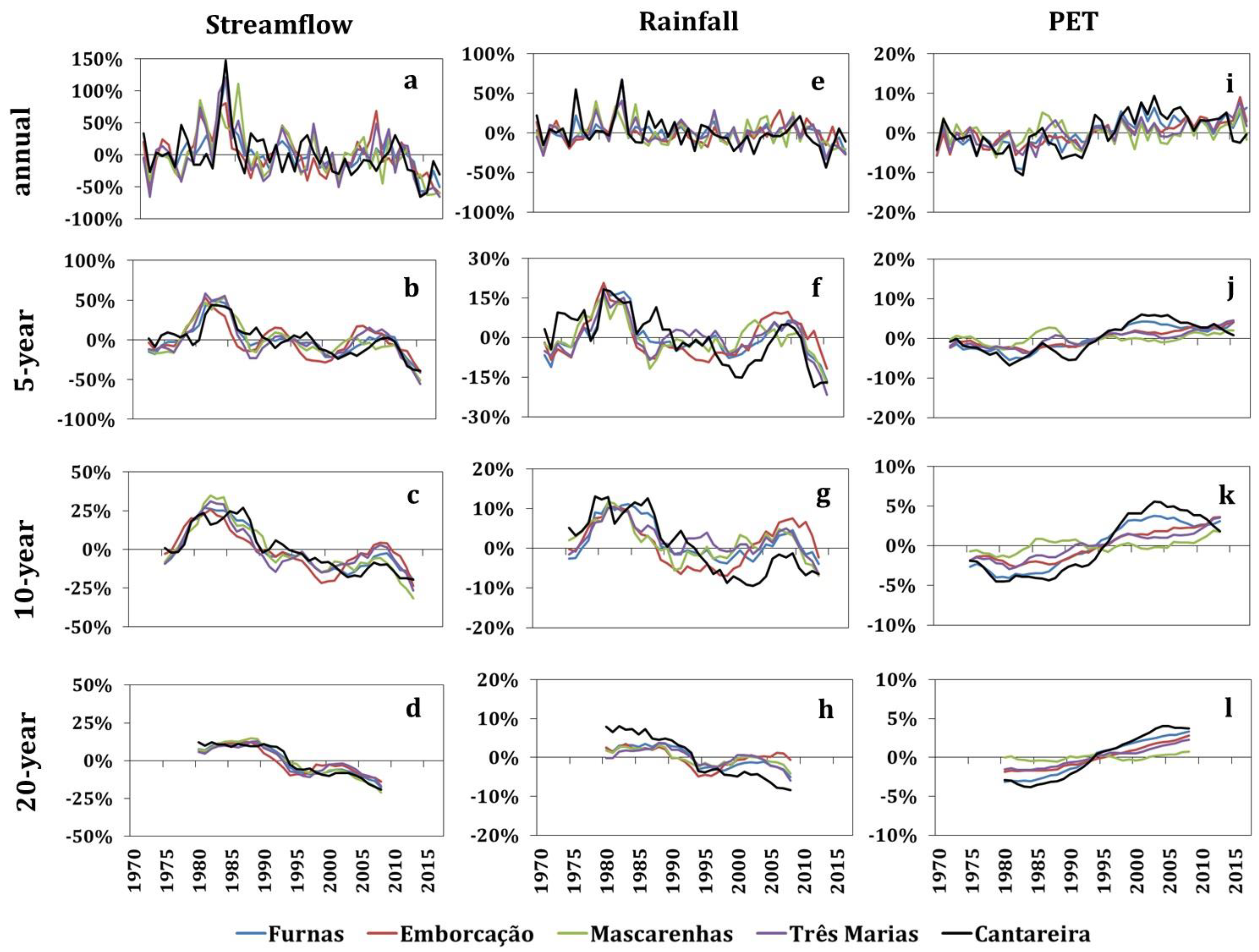
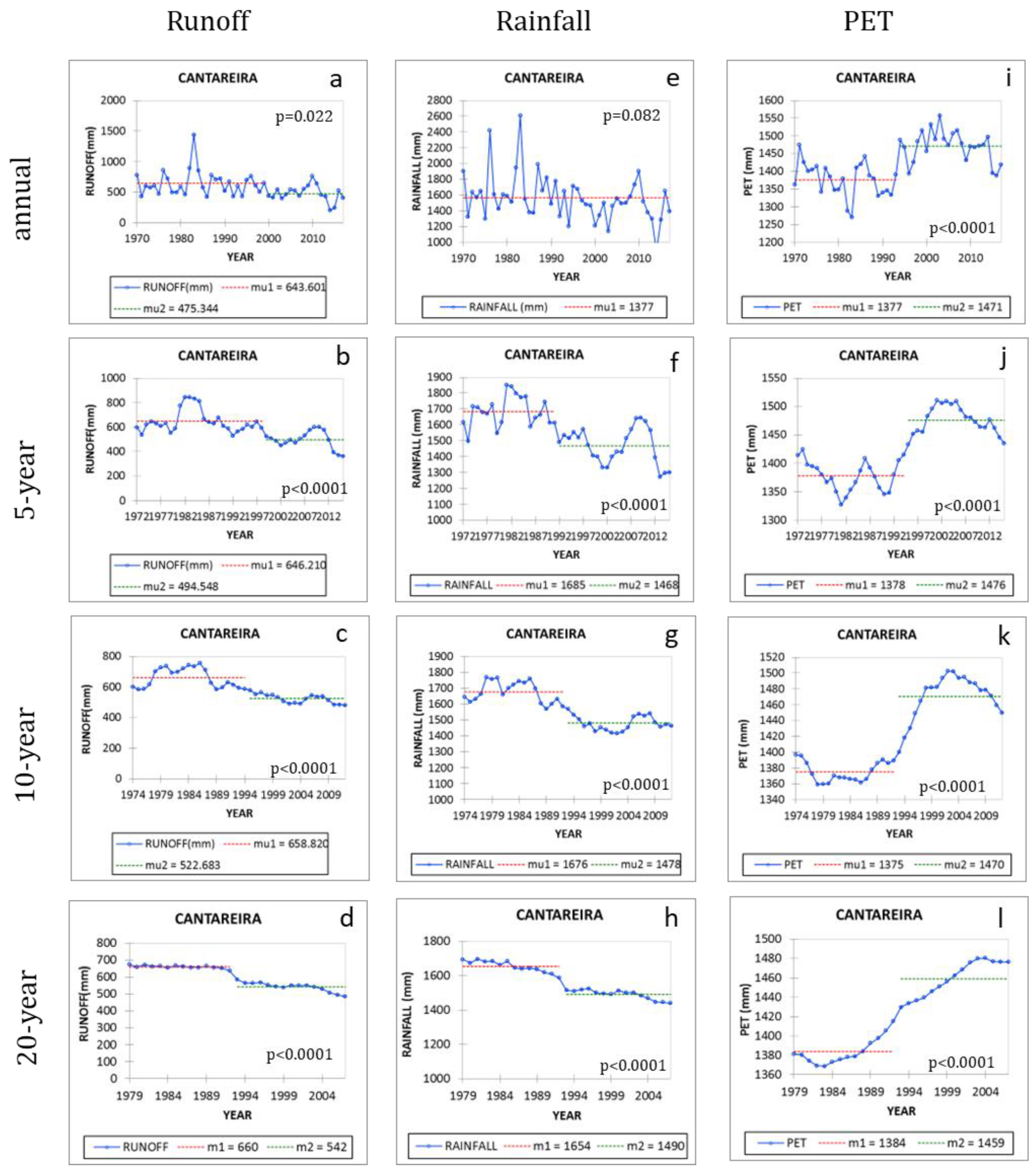
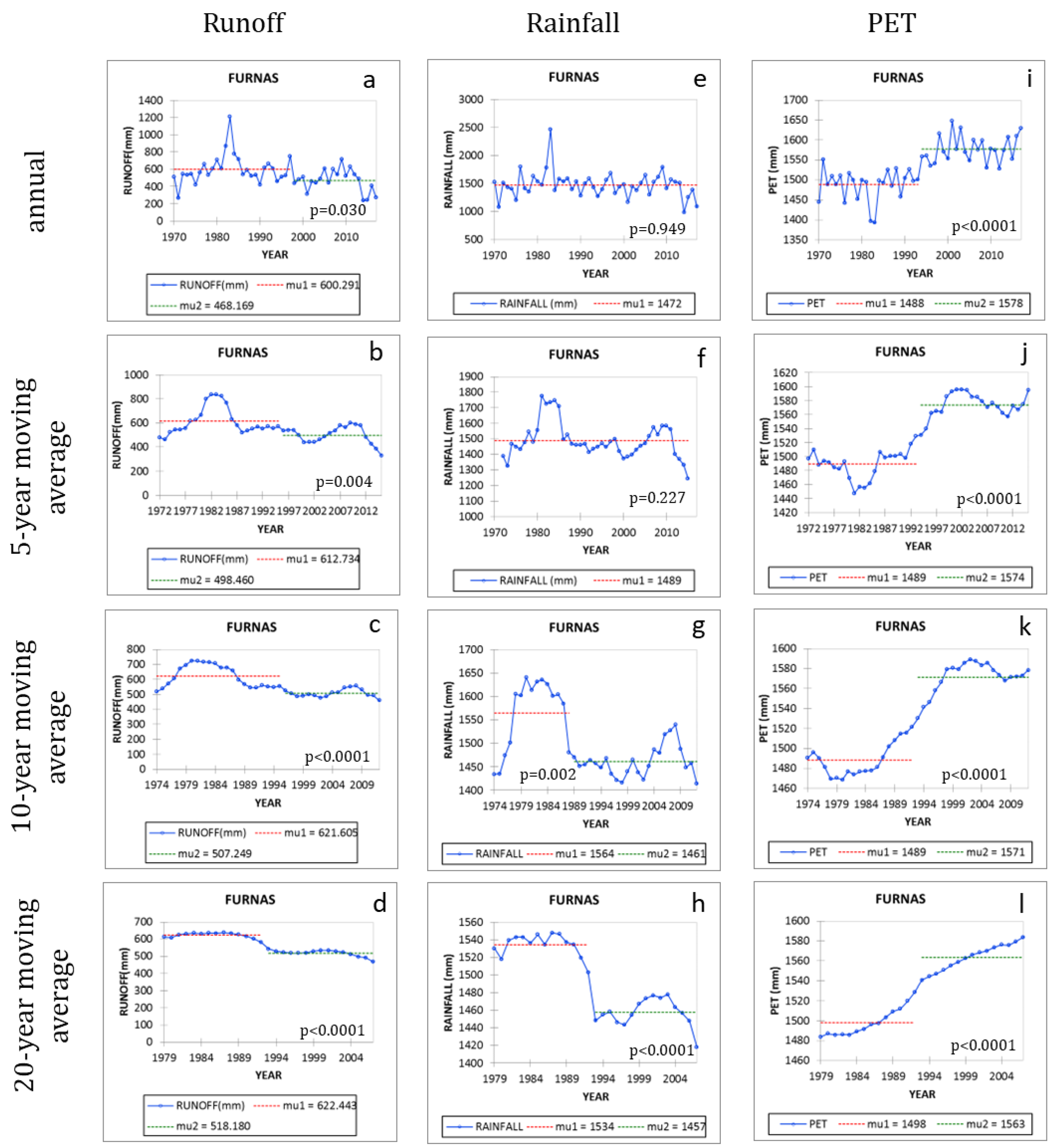
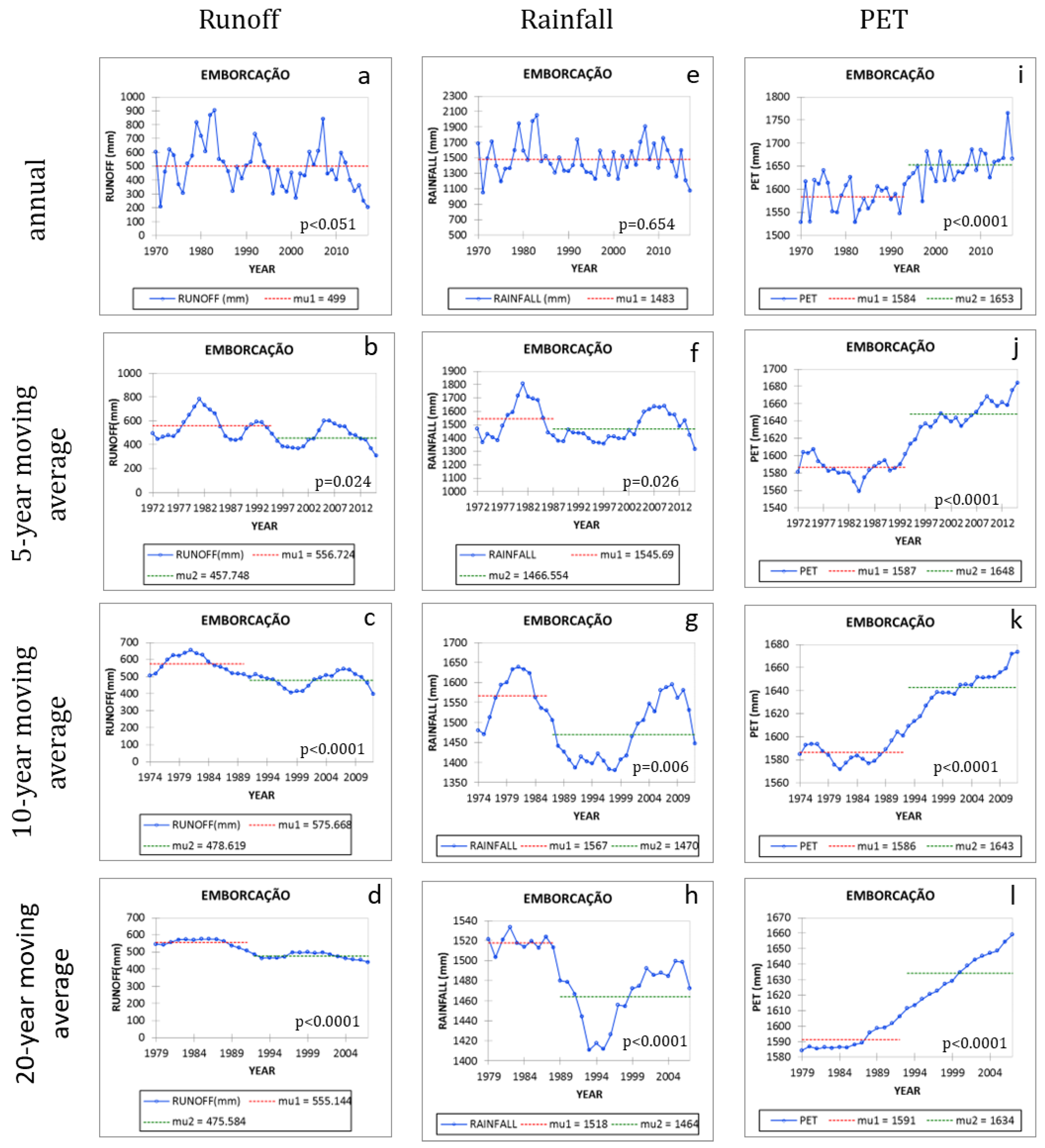
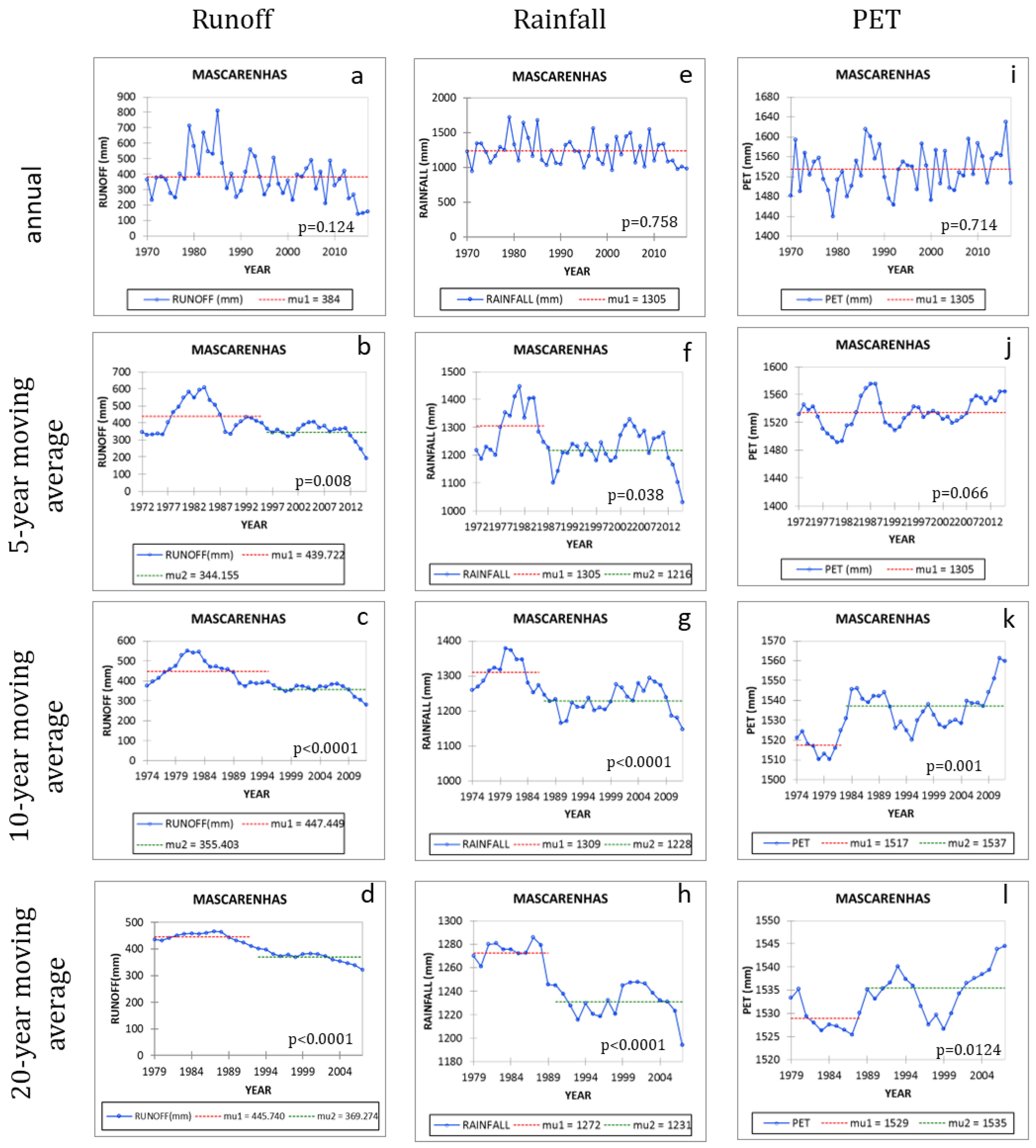
3.1. Time-Series and Trend Analysis of Hydroclimate Variables

Figure 3a–d depicts the historical anomalies for streamflow, rainfall (e–h) and potential evapotranspiration (i–l) in annual and 5-, 10- and 20-year moving averages. A negative trend was detected in streamflow (Z-value < 0) for all studied basins in all time steps (

Table 2. Results of the Mann–Kendall test, Z-value, and significance (p-value) and the Pettitt test for streamflow, rainfall and potential evapotranspiration (PET) for Brazilian Southeast watersheds in annual and 5-, 10- and 20-years moving average. Only significant break points (p < 0.05) are shown.

		Runoff			Rainfall			PET
		Z-Value	(p-Value)	BP	Z-Value	(p-Value)	BP	Z-Value	(p-Value)	BP
Annual	FUR	−0.223	(0.026) *	1997	−0.082	(0.419)	-	0.559	(<0.0001) *	1993
	EMB	−0.245	(0.015) *	-	−0.057	(0.576)	-	0.535	(<0.0001) *	1993
	MAS	−0.202	(0.044) *	-	−0.142	(0.158)	-	0.135	(0.180)	-
	TM	−0.161	(0.108)	-	−0.094	(0.351)	-	0.441	(<0.0001) *	1993
	CAN	−0.271	(0.007) *	1999	−0.223	(0.026) *	-	0.326	(<0.0001) *	1993
5-Year	FUR	−0.271	(0.010) *	1995	−0.129	(0.221)	-	0.581	(<0.0001) *	1993
	EMB	−0.239	(0.023) *	1995	−0.111	(0.9114)	1995	0.683	(<0.0001) *	1993
	MAS	−0.298	(0.004) *	1995	−0.182	(0.084)	1986	0.266	(0.011) *	-
	TM	−0.154	(0.142)	-	−0.078	(0.460)	-	0.648	(<0.0001) *	1994
	CAN	−0.469	(<0.0001) *	1998	−0.482	(<0.0001) *	1991	0.427	(<0.0001) *	1994
10-Year	FUR	−0.522	(<0.0001) *	1995	−0.266	(0.018) *	1988	0.676	(<0.0001) *	1992
	EMB	−0.455	(<0.0001) *	1990	−0.085	(0.453)	1986	0.776	(<0.0001) *	1992
	MAS	−0.601	(<0.0001) *	1995	−0.323	(0.004) *	1986	0.387	(0.001) *	1982
	TM	−0.379	(0.001) *	1989	−0.333	(0.003) *	1987	0.811	(<0.0001) *	1994
	CAN	−0.646	(<0.0001) *	1994	−0.576	(<0.0001) *	1992	0.582	(<0.0001) *	1992
20-Year	FUR	−0.66	(<0.0001) *	1992	−0.507	(0.000) *	1992	0.975	(<0.0001) *	1992
	EMB	−0.621	(<0.0001) *	1991	−0.305	(0.021) *	1988	0.961	(<0.0001) *	1992
	MAS	−0.714	(<0.0001) *	1992	−0.468	(0.000) *	1989	0.424	(0.001) *	1988
	TM	−0.567	(<0.0001) *	1992	−0.443	(0.001) *	1991	0.921	(<0.0001) *	1992
	CAN	−0.837	(<0.0001) *	1992	−0.882	(<0.0001) *	1992	0.862	(<0.0001) *	1992

Note: * Statistically significant trends at 95% confidence level for Mann-Kendall test. FUR: Furnas, EMB: Emborcação, MAS: Mascarenhas, TM: Três Marias, CAN: Cantareira and BP: break point.

). Decreases were statistically significant (p < 0.05) for all time steps, except for Três Marias basin in an annual time step and 5-year moving average. Table 2 shows that significant break points, from 1989 to 1999, were detected in the streamflow dataset in most of the cases. Only significant break points (p < 0.05) are shown in Table 2. For the annual analysis, only the Furnas and Cantareira systems showed a significant break point at 1997 (p = 0.03) and 1999 (p = 0.02), respectively. For 20-year moving averages (

Table 3. Mean values for streamflow (Q), rainfall (P) and potential evapotranspiration (PET) in mm for pre- and post-break point periods according to Pettitt test for Brazilian Southeast watersheds in 20-year moving averages.

		Pre BP		Pos BP		∆	p-Value
		Mean	Period	Mean	Period
CAN	Q	660	(1970–1992)	542	(1993–2017)	−18%	<0.0001
	P	1654	(1970–1992)	1490	(1993–2017)	−10%	<0.0001
	PET	1384	(1970–1992)	1459	(1993–2017)	5%	<0.0001
FUR	Q	622	(1970–1992)	518	(1993–2017)	−17%	<0.0001
	P	1534	(1970–1992)	1457	(1993–2017)	−5%	<0.0001
	PET	1498	(1970–1992)	1563	(1993–2017)	4%	<0.0001
EMB	Q	555	(1970–1991)	476	(1992–2017)	−14%	<0.0001
	P	1518	(1970–1988)	1464	(1989–2017)	−4%	<0.0001
	PET	1591	(1970–1992)	1634	(1993–2017)	3%	<0.0001
MAS	Q	446	(1970–1992)	369	(1993–2017)	−17%	<0.0001
	P	1272	(1970–1989)	1231	(1990–2017)	−3%	0.012
	PET	1529	(1970–1988)	1535	(1989–2017)	0.4%	<0.0001
TM	Q	460	(1970–1992)	395	(1993–2017)	−14%	<0.0001
	P	1448	(1970–1991)	1402	(1992–2017)	−3%	<0.0001
	PET	1588	(1970–1992)	1623	(1993–2017)	2%	<0.0001

Note: ∆ represent ratios of change. FUR: Furnas, EMB: Emborcação, MAS: Mascarenhas, TM: Três Marias and CAN: Cantareira.

), differences in the mean streamflow values between the sub-periods ranged from −14% to a −18%. For this aggregation time, the Cantareira system yielded the highest ratio of change. The break point period was 1992 (the central year of the period 1983–2002) and mean value for the pre-break point being 660 mm and 542 mm being the post-break mean. Mean values of sub-periods for other time steps could be found in Figure A1, Figure A2, Figure A3, Figure A4 and Figure A5 of Appendix B.

A negative trend was detected in rainfall dataset for all studied basins. Decreases were significant mainly for the 10- and 20-year moving averages (Table 2). Significant break points, from 1986 to 1992, were detected in rainfall dataset in most of the cases. Analysing 20-year moving averages (Table 3), differences in the mean rainfall values between the sub-periods ranged from −3% to a −10%. Cantareira system yielded the highest ratio of change. The break point period was 1992, being 1654 mm the mean value for the pre-break period and 1490 mm for the post-break period.

A positive trend was detected in the PET dataset for all studied basins in all aggregation times. Increases were statistically significant for all moving averages (Table 2), except for Mascarenhas basin in the annual analysis. Table 2 shows that significant break points, from 1988 to 1994, were detected in PET dataset in most of the cases. Analysing 20-year moving averages (Table 3), differences in mean PET values between the sub-periods ranged from 0.4% to a 5%. Again, the Cantareira system yielded the highest ratio of change. The break point period was once again 1992. The mean value for the pre-break and post-break periods were 1384 mm and 1459 mm, respectively.

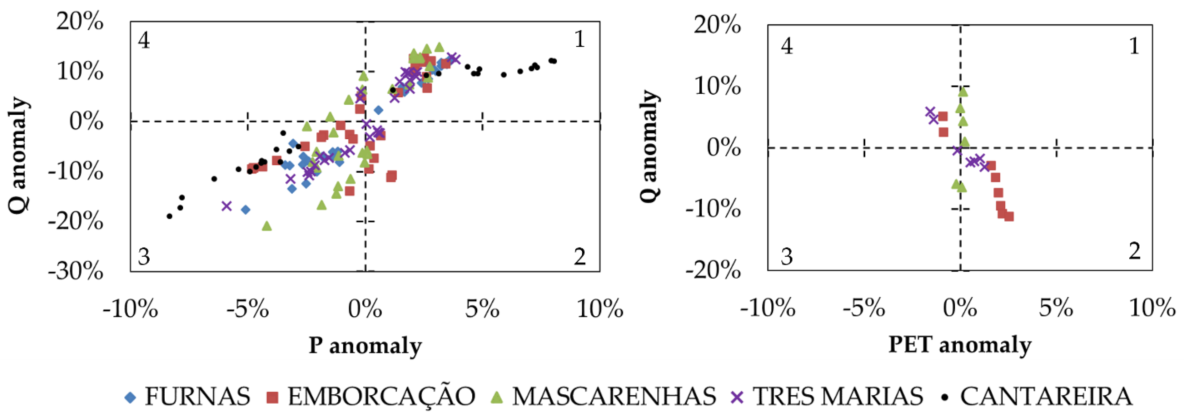
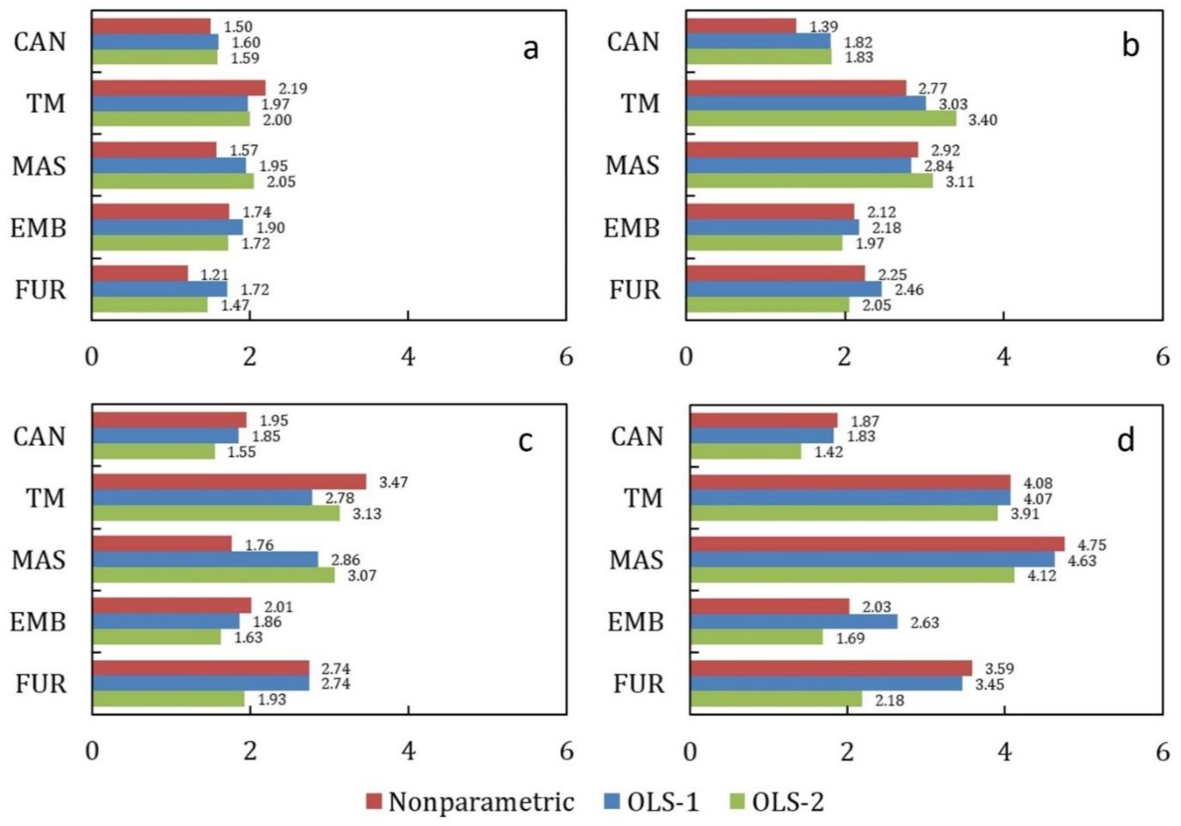
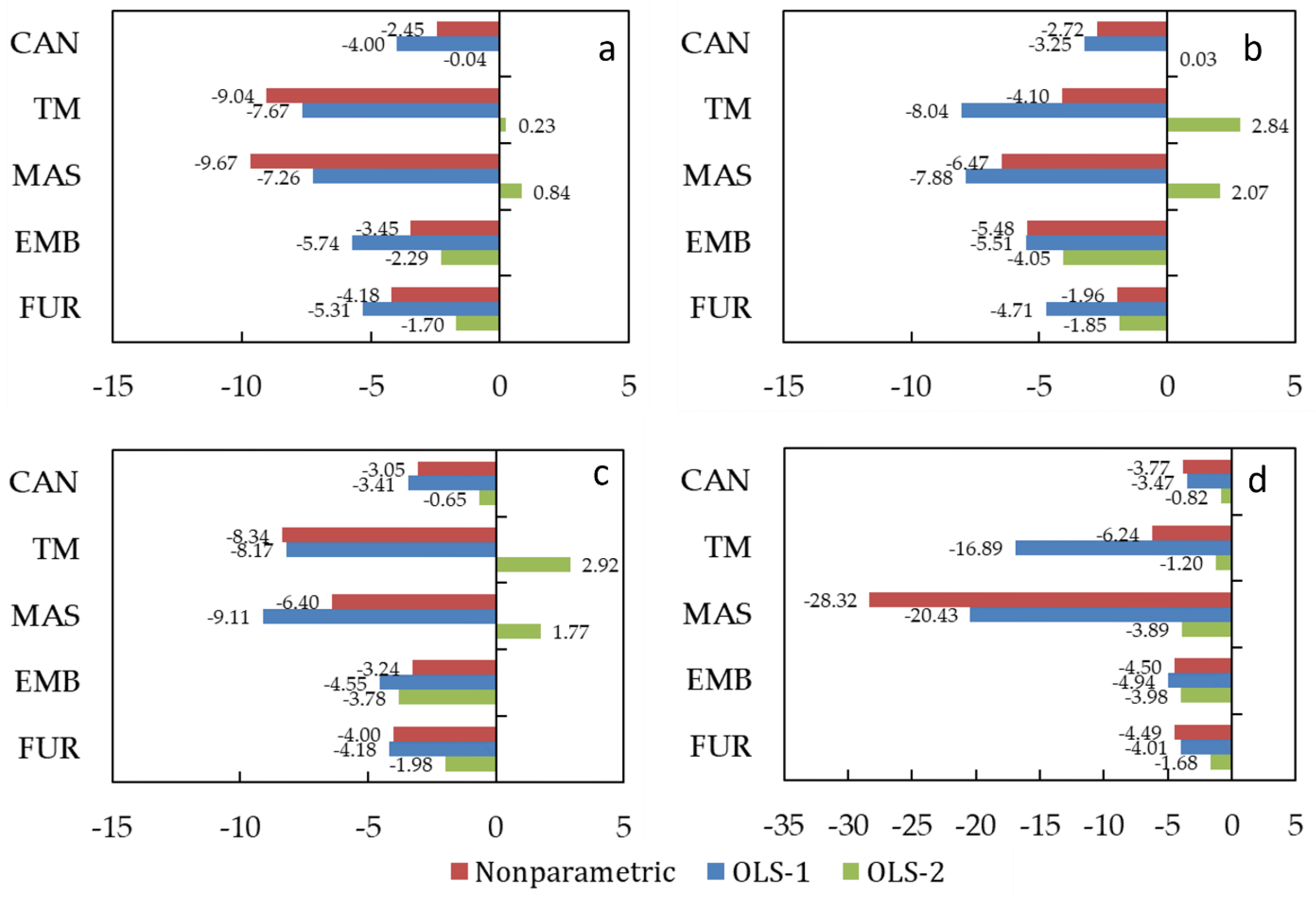
3.2. Elasticity Results

Figure 4 shows the relationship between P and Q historical anomalies for all the basins considering 20-year moving average. It encloses all the information, i.e., 29 data of the 20-year moving average for each basin. As expected, most of the P and Q anomalies occurred in the same direction, i.e., positive P and positive Q (Figure 4, quadrant 1) or negative P and negative Q (Figure 4, quadrant 3). Major positive P anomalies were detected up to 5% (except for Cantareira system) associated with up to 15% positive (Figure 4, quadrant 1) and negative Q anomalies (Figure 4, quadrant 2). Major negative P anomalies were detected up to 5% (except for Cantareira system) associated with up to 10% positive (Figure 4, quadrant 4) and 20% negative Q anomalies (Figure 4, quadrant 3). For the first quadrant, the closer the dispersion is to the angle 0° (to the vertical line), the more sensitive the streamflow, the closer to angle 90° (to the horizontal line), more resilient the streamflow.

Some anomaly relationships occurred in opposite directions, i.e., positive P and negative Q (Figure 4, quadrant 2) or negative P and positive Q (Figure 4, quadrant 4). These opposing signs observed for P and Q anomalies only occurred for low P anomalies. In those situations, PET anomalies play a greater influence on the Q response (Figure 4), which may result in opposing signs for P and Q anomalies. This dynamic can be influenced, besides climate variability, by the availability of water in the soil. In order to clarify relationships between those anomalies, Figure 4 includes only data within which P and Q anomalies occurred in opposite directions. Cantareira and Furnas did not show any such relationship. Emborcação yielded the highest PET anomalies, which may justify its greater Q anomalies. For Mascarenhas, PET anomalies could not explain the opposing relationship between Q and P anomalies, which raises the hypothesis of other climatological variables influencing the Q dynamics, as well as land use and land cover changes.

The εp results are presented in Figure 5. For annual analysis (Figure 5a), εp ranged from 1.21, in Furnas, to 2.19, in Três Marias, meaning that a 10% rainfall anomaly induced from 12.1% to 21.9% of the Q anomalies. Q anomalies respond directly to P anomalies; however, basins present a hydrological memory that stores the P anomalies, as well as other physical variables over a certain period [60]. Considering this hydrological memory, the analyses for 5-year (Figure 5b), 10-year (Figure 5c) and 20-year (Figure 5d) moving averages revealed higher εp values, although a slight increment is detected. For the 5-year aggregation time, εp ranged from 1.39, in Cantareira system, to 3.40, in Três Marias. For the 10-year aggregation time, εp ranged from 1.55, in Cantareira system, to 3.47, in Três Marias. For the 20-year aggregation time, εp ranged from 1.42, in Cantareira system, to 4.75, in Mascarenhas. In general, Mascarenhas and Três Marias basins yielded the highest εp values.

Results for εpet are shown in Figure 6. In climate areas similar to SEB, the higher the PET, the greater the water volume that evaporates and therefore the smaller the water volume that remains to be drained. Therefore, εpet is generally negative. For the NP and OLS-1 methods, in the annual time step (Figure 6a), εpet ranged from −2.45 for Cantareira and −9.67 for Mascarenhas. These values implies that 1% increase in PET leads to streamflow decreases ranging from 2.45% to 9.67%. For 5-year aggregation time, εpet ranged between −1.96 for Furnas to −8.04 for Três Marias. For the 10-year aggregation time, εpet ranged between −3.05 for the Cantareira system to −9.11 for Mascarenhas. For the 20-year aggregation time, εpet ranged from −3.47 for Cantareira system to −28.3 for Mascarenhas.

With the OLS-2 method, absolute values of εpet were generally lower than those obtained by the other methods and, in some cases, presented positive values. This is because this method computes the influence of PET and P anomalies, and P influence (directly proportional) could be greater than the PET influence (inversely proportional) to the Q response. Três Marias and Mascarenhas exhibited positive values for annual analysis (0.23 and 0.84), 5-year (2.84 and 2.07) and 10-year (2.92 and 1.77, respectively) aggregation times. For Cantareira system, Furnas and Emborcação values ranged from −0.04 to −2.29 for annual analysis. Considering 5-year moving averages, values ranged from −1.85 to −4.05; in 10-year analysis figures were between −0.65 to −3.78. For 20-year aggregation time, εpet values were negative for all watersheds ranged from −0.82, in Cantareira system, to −3.98, in Emborcação.

4. Discussion

4.1. Trends in Climate Variables

The negative trend in streamflow observed in the last 48 years in all five basins was unprecedented in the recent SEB history. This may have been caused by a variety of climatological factors that led to lower rainfall and higher PET (both trends also detected in this study), such as, changes in rainfall seasonality or lack of extremely high rainfall events. In a drought indicators analysis in Brazil [61], the authors found that the last decade (2011–2021) recorded the highest recurrence of severe droughts since 1981. The authors also suggest that droughts are more intense and frequent due to the compound effect of decreased precipitation and increased in temperature in a possible global warming scenario. The decreased precipitation and increased surface temperature result in the increased evapotranspiration and decreased soil moisture, leading to negative feedback processes that exacerbate drought events [61]. In a monthly precipitation assessment from 1961 to 2011 in Southeastern Brazil, non-significant trends were detected, but significant positive trends in mean temperature, as well as in PET for all months of that period were detected [48]. In contradict, our analysis showed significant negative trends in precipitation for SEB, corroborating those results detected in another study for the period 1979–2011 [6]. Although a significant negative trend in rainfall was detected only in Cantareira system in the annual analysis in this study, the significance of the trends was stronger when longer aggregation time were applied. This is because the interannual variability is smoothed and trends become clear.

It is remarkable that the smallest basin, the Cantareira system, yielded the greatest absolute Z-value in streamflow trend (Table 3). Despite a high interannual variability (Figure 3a), which is expected for smaller basins, a significant negative trend in streamflow was detected even in the annual analysis. Negative trend in two sub-basins (out of four) of the Cantareira System was reported in another study [62] when considering annual precipitation time series. The region is surrounded by deforested areas now dedicated to reforestation/silviculture. Indeed, this basin is located very close to the biggest metropolitan region of South America, which has experienced an expressive growth in the last decades, becoming a very distinct heat island [33]. The accumulation of these factors could explain the PET positive trend.

Although significant trends in streamflow were followed by significant trends in PET even in annual analyses, it may be also associated with land uses and land cover changes (LULCC), that lead to disturbances in the atmosphere-surface cover-groundwater relationship, such as replacement of forests by urbanized areas and pastures and vice versa [1]. In another study for Cantareira System, human activities played a more significant impact on streamflow reduction than climate variability [62]; however, the period analysed in that study is shorter and the most anomalous years of the 2010’s were not considered, which may downplayed the importance of climatic variables. Nevertheless, research with an extended data period including the last decade and addressing climatological and physical factors, which were beyond the scope of this study, are encouraged.

Future climate projections [63] indicate that for the eastern portion of Southeastern Brazil, characterized by the Atlantic Forest biome, rainfall is expected to increase by the end of the next decade—however, the reliability of this projection is low. For the western portion, characterized by the Cerrado biome, a reduction in rainfall is expected for the end of the next decade, corroborating the results found in this study for the past climate observations. In addition to reduced rainfall, an increase in the frequency/intensity of heavy precipitation episodes, separated by longer dry seasons [64] is also projected. This suggests intense storms with impacts to the population exposed to landslides and flash floods, and sequence of consecutive dry days that can produce heat waves and dry conditions leading to flash droughts [65] and water insecurity.

4.2. Elasticity of Streamflow

The analysis of elasticity showed the cumulative effect of climatological variations in streamflow—elasticity increases as the aggregation time increases as a hydrological response. For example, in a given year a certain amount of rainfall is stored as groundwater and influences the streamflow to a low degree in that same year and hence elasticity is small. The water stored as groundwater will affect streamflow in a later year not computed in the analysis, apparently raising elasticity. This mechanism is similar to the propagation of droughts in the hydrological cycle, which increases the water deficit in groundwater sometime after the rainfall anomaly. A global study of streamflow elasticity to precipitation assessment [13] also noticed an increase in εp values with aggregation time (named as positive scaling), from monthly to multiannual timescales. In that global study, in monthly to annual aggregation intervals, εp values increased considerably, while in annual to multiyear (up to 5-year) aggregation intervals, εp presented a slight increase approaching 1.5. In the present, study a slight increase in εp values was detected with increasing temporal aggregation intervals, but the increases were stronger for εpet. Indeed, in that study, more arid/less rainy basins showed, more frequently, a positive scaling of the streamflow elasticity to precipitation with aggregation time. The authors thought that the reason could be associated with higher εp values. This pattern was also observed in our study at less the rainy basins, Mascarenhas and Três Marias, showing higher positive scaling. For this reason, elasticity should be assessed and interpreted conditioned to the time scale of interest under changing climate conditions, where variables vary dynamically with different time scales.

Mascarenhas and Três Marias watershed yielded higher ε values. PET anomalies in Mascarenhas were the only ones to show a non-significant trend among the annual analyses. Despite that, Q anomalies followed a significantly negative trend similar to those of the other basins, reflecting in the high εpet values. Even for εp, Mascarenhas and Três Marias yielded the highest values, especially considering 20-years aggregate time.

In relation to the methods used to estimate streamflow elasticity, there is a numerical problem with the NP method (see Equation (3)) when the value of the climate variable ($X_t)$ approaches to the mean value ($\overline{X})$, causing the ε to approach infinity [14]. Therefore, it is necessary to carefully analyze the εpet value obtained for Mascarenhas. Although this value may be overestimated, εpet calculated through the OLS-1 method, which does not present such numerical problem, was also high.

Mascarenhas and Três Marias yielded the lowest runoff indexes (0.31 and 0.29, respectively, Table 1) and highest aridity indexes (1.25 and 1.16, respectively). These results corroborate those reported in Australia [22], with less rainy basins presenting higher ε, i.e., there is a negative correlation between ε and runoff index. This correlation occurs because the runoff is driven more directly by the P anomalies, with temperature (through PET) anomalies having a minor role. In a trend analysis of the hydroclimate variables in China [1] annual streamflow was more sensitive to annual temperature in arid basins in comparison to more humid basins, which is a result similar to those reported in this study. Moreover, due to the nonlinearity of the P and Q relationship, the same absolute change in streamflow for a given absolute change in precipitation would be reflected as a higher εp in a basin with a lower runoff coefficient [18].

The Cantareira System yielded the highest P and Q anomalies in the 1970–2017 period, although the correspondent elasticity value was low and did not stand out among those obtained for the other basins. Thus, it is important to highlight that ε does not refer to absolute anomaly values. In an annual analysis for the 1976–2009 period, slightly higher εp values were reported [62], ranging from 1.85 to 2.4, for two sub-basins of the Cantareira System, and lower εpet values, between −0.85 to −1.42, when compared to those reported here. The different time periods (1976–2009 versus 1970–2017) could explain the differences observed in ε values. Due to its large negative Q trend and water consumption (downstream of the gauge station) close to the water production, Cantareira experienced its worst hydrological drought in 2014 and 2016 with a serious water shortage [31], which led to its worldwide prominence in the water crisis context.

In a global εp estimative noted that values tend to be low (below 2) when annual streamflow or precipitation are high (near 1500 mm) [18], which is the case of the basins here studied. Our study areas are inserted in climate zones Aw and Cw, which were found in that global study [18] to present εp in the range of 0.9–3.3 (median 2.0) and 0.8–2.8 (median 1.8) respectively, calculated using annual data. For this aggregation time, we found εp ranging between 1.2 and 2.2, in good agreement with the global study.

5. Uncertainty and the Limitations

Rainfall gauge stations are not well distributed spatially. There are areas not covered by the monitoring network, especially in the Emborcação basin, which can affect the estimation of climate sensitivity. Although the minimum data length suggested for computing elasticity is 20 years, longer time series are preferred [1]. Unfortunately, data for the studied region began in 1970. Short time series might lead to high variability and high estimates of elasticity [27].

A major shortcoming of the NP method to estimate the elasticity is that the change in streamflow due to human activities cannot be expressed explicitly in terms of elasticity coefficients. Physical changes in land use are beyond the scope of this article. Empirical indicators of elasticity, as those adopted in this paper, are calculated using observed data and therefore may represent anomalies in concurrent climate situations, which makes it more difficult to attribute Q anomalies to specific climate variables. Moreover, they only represent changes already observed in the past, meaning that extrapolations towards the future should be interpreted with caution [20]. Results of this paper point out that the studied strategic basins in SEB, for hydropower generation and water supply, are very sensitive to climate variations. These findings can support strategic government decisions and can be beneficial to the strategic planning of climate change adaptation measures, drought managing, and water security.

6. Conclusions

The trends of hydro-climatological variables were assessed in this study for five important basins located in the Southeastern Brazil: Furnas, Emborcação, Mascarenhas, Três Marias and the Cantareira System, considering the 1970–2017 period. Trend analysis was performed using annual and aggregation times of 5-, 10- and 20-years. It was possible to observe a clear negative trend of streamflow during these 48 years. The analysis also detected a positive trend in PET and a negative trend in rainfall for all basins for most of the aggregation times. According to non-parametric Pettitt test, there is a year (or period) at which there is a change in Q, P and PET data for most of the aggregation times. Significant break points of the time series were detected between 1986 to 1999 in most of the cases.

The concept of elasticity was used to examine the streamflow sensitivity to variations in climate variables. For annual analysis of the streamflow elasticity to rainfall revealed that 1% decrease in rainfall resulted in 1% to 2% reduction in streamflow, while 1% increase in potential evapotranspiration induced different reductions in streamflow, ranging from 1% to 9%. Elasticity analysis considering longer aggregation times—in this case, the analysis of 20-year moving averages, revealed that impacts on the streamflow were cumulative: 1% decrease in rainfall resulted in 2% to 5% reduction in streamflow, while 1% increase in potential evapotranspiration induced 4% to 28% decrease in streamflow. This different temporal response may be associated with the hydrological memory of the basins: hydrological processes, when considering longer time scales, “remember” past atmospheric conditions and their impacts are reflected in subsequent events. In addition, streamflow dynamics was more sensitive to variations in PET than in precipitation.

The Três Marias and Mascarenhas basins yielded the highest elasticity values, as well as the lowest runoff and aridity indexes, which corroborates the concept of more sensitive streamflow in less rainy basins. The Cantareira System did not yield high elasticity values, although its rainfall and potential evapotranspiration anomalies were significant over the years (the largest in this study), which lead the streamflow production to reach critical levels, corroborating the severe water crisis in the years 2014 to 2016. Considering the economic importance of SEB to the Gross Domestic Product of the country and for the water supply of the Metropolitan Region of São Paulo City, the Cantareira System is here highlighted, due to its greatest streamflow changes.

Although droughts are not new in Brazil, the drought events in Southeastern Brazil have come as a surprise to the region affected, not only for the immediate effects, but also for the associated long-term impacts. This new climate conditions have forced decision makers to rethink public policies and management plans. Studies similar to ours can be the basis for the management of water resources aiming at water security, indicating the most elastic basins to climatic variations and pointing out where to allocate financial and human resources. Water resource planning and management must incorporate the impacts of climate variability in order to secure future water supplies.

References

1. Wu, J.; Wang, Z.; Dong, Z.; Tang, Q.; Lv, X.; Dong, G. Analysis of natural streamflow variation and its influential factors on the yellow river from 1957 to 2010. Water 2018, 10, 1155. [Google Scholar] [CrossRef] [Green Version]
2. Kibria, K.N.; Ahiablame, L.; Hay, C.; Djira, G. Streamflow trends and responses to climate variability and land cover change in South Dakota. Hydrology 2016, 3, 2. [Google Scholar] [CrossRef] [Green Version]
3. Burn, D.H.; Elnur, M.A.H. Detection of hydrologic trends and variability. J. Hydrol. 2002, 255, 107–122. [Google Scholar] [CrossRef]
4. Sun, T.; Ferreira, V.G.; He, X.; Andam-Akorful, S.A. Water Availability of São Francisco River Basin Based on a Space-Borne Geodetic Sensor. Water 2016, 8, 213. [Google Scholar] [CrossRef]
5. Li, E.; Mu, X.; Zhao, G.; Gao, P.; Shao, H. Variation of runoff and precipitation in the hekou-longmen region of the yellow river based on elasticity analysis. Sci. World J. 2014, 2014, 1–11. [Google Scholar] [CrossRef] [PubMed]
6. Rao, V.B.; Franchito, S.H.; Santo, C.M.E.; Gan, M.A. An update on the rainfall characteristics of Brazil: Seasonal variations and trends in 1979–2011. Int. J. Climatol. 2016, 36, 291–302. [Google Scholar] [CrossRef]
7. Dobrovolski, R.; Rattis, L. Water collapse in Brazil: The danger of relying on what you neglect. Nat. Conserv. 2015, 13, 80–83. [Google Scholar] [CrossRef] [Green Version]
8. Rodrigues, R.R.; Taschetto, A.S.; Sen Gupta, A.; Foltz, G.R. Common cause for severe droughts in South America and marine heatwaves in the South Atlantic. Nat. Geosci. 2019, 12, 620–626. [Google Scholar] [CrossRef]
9. Tan, M.L.; Ibrahim, A.L.; Yusop, Z.; Duan, Z.; Ling, L. Impacts of land-use and climate variability on hydrological components in the Johor River basin, Malaysia. Hydrol. Sci. J. 2015, 60, 873–889. [Google Scholar] [CrossRef]
10. Wei, X.; Liu, W.; Zhou, P. Quantifying the relative contributions of forest change and climatic variability to hydrology in large watersheds: A critical review of research methods. Water 2013, 5, 728–746. [Google Scholar] [CrossRef]
11. Wilson, D.; Hisdal, H.; Lawrence, D. Has streamflow changed in the Nordic countries?—Recent trends and comparisons to hydrological projections. J. Hydrol. 2010, 394, 334–346. [Google Scholar] [CrossRef]
12. Schaake, J.C. From climate to flow. Clim. Chang. US Water Resour. 1990, 5, 177–206. [Google Scholar]
13. Zhang, Y.; Viglione, A.; Blöschl, G. Temporal Scaling of Streamflow Elasticity to Precipitation: A Global Analysis. Water Resour. Res. 2022, 58, e2021WR030601. [Google Scholar] [CrossRef]
14. Sankarasubramanian, A.; Vogel, R.M.; Limbrunner, J.F. Climate elasticity of streamflow in the United States. Water Resour. Res. 2001, 37, 1771–1781. [Google Scholar] [CrossRef]
15. Chiew, F.H.S.; Potter, N.J.; Vaze, J.; Petheram, C.; Zhang, L.; Teng, J.; Post, D.A. Observed hydrologic non-stationarity in far south-eastern Australia: Implications for modelling and prediction. Stoch. Environ. Res. Risk Assess. 2014, 28, 3–15. [Google Scholar] [CrossRef]
16. Sun, S.; Chen, H.; Ju, W.; Song, J.; Zhang, H.; Sun, J.; Fang, Y. Effects of climate change on annual streamflow using climate elasticity in Poyang Lake Basin, China. Theor. Appl. Climatol. 2013, 112, 169–183. [Google Scholar] [CrossRef]
17. Kim, B.S.; Hong, S.J.; Lee, H.D. The potential effects of climate change on streamfow in rivers basin of korea using rainfall elasticity. Environ. Eng. Res. 2013, 18, 9–20. [Google Scholar] [CrossRef]
18. Chiew, F.H.S.; Peel, M.C.; McMahon, T.A.; Siriwardena, L.W. Precipitation elasticity of streamflow in catchments across the world. In Climate Variability and Change—Hydrological Impacts; Demuth, S., Gustard, A., Planos, E., Scatena, F., Servat, E., Eds.; IAHS Press: Wallingford, UK, 2006; pp. 256–262. [Google Scholar]
19. Mohor, G.S.; Rodriguez, D.A.; Tomasella, J.; Siqueira Júnior, J.L. Exploratory analyses for the assessment of climate change impacts on the energy production in an Amazon run-of-river hydropower plant. J. Hydrol. Reg. Stud. 2015, 4, 41–59. [Google Scholar] [CrossRef] [Green Version]
20. Andréassian, V.; Coron, L.; Lerat, J.; Le Moine, N. Climate elasticity of streamflow revisited—An elasticity index based on long-term hydrometeorological records. Hydrol. Earth Syst. Sci. 2016, 20, 4503–4524. [Google Scholar] [CrossRef] [Green Version]
21. Seymenov, K. Climate Elasticity of Annual Streamflow in Northwest Bulgaria. In Smart Geography; Springer: Berlin, Germany, 2020; pp. 105–115. [Google Scholar] [CrossRef]
22. Chiew, F.H.S. Estimation of rainfall elasticity of streamflow in Australia. Hydrol. Sci. J. 2006, 51, 613–625. [Google Scholar] [CrossRef]
23. Liu, N.; Harper, R.J.; Smettem, K.R.J.; Dell, B.; Liu, S. Responses of streamflow to vegetation and climate change in southwestern Australia. J. Hydrol. 2019, 572, 761–770. [Google Scholar] [CrossRef]
24. Ribeiro Neto, A.; da Paz, A.R.; Marengo, J.A.; Chou, S.C. Hydrological Processes and Climate Change in Hydrographic Regions of Brazil. J. Water Resour. Prot. 2016, 8, 1103–1127. [Google Scholar] [CrossRef] [Green Version]
25. Potter, N.J.; Petheram, C.; Zhang, L. Sensitivity of streamflow to rainfall and temperature in south-eastern Australia during the Millennium drought. In Proceedings of the 19th International Congress on Modelling and Simulation, Perth, Australia, 12–16 December 2011; pp. 3636–3642. [Google Scholar]
26. Hu, S.; Liu, C.; Zheng, H.; Wang, Z.; Yu, J. Assessing the impacts of climate variability and human activities on streamflow in the water source area of Baiyangdian Lake. J. Geogr. Sci. 2012, 22, 895–905. [Google Scholar] [CrossRef]
27. Gong, X.; Xu, A.; Du, S.; Zhou, Y. Spatiotemporal variations in the elasticity of runoff to climate change and catchment characteristics with multi-timescales across the contiguous United States. J. Water Clim. Chang. 2022, 13, 1408–1424. [Google Scholar] [CrossRef]
28. Geirinhas, J.L.; Trigo, R.M.; Libonati, R.; Coelho, C.A.S.; Palmeira, A.C. Climatic and synoptic characterization of heat waves in Brazil. Int. J. Climatol. 2018, 38, 1760–1776. [Google Scholar] [CrossRef]
29. Cunha, A.P.M.A.; Zeri, M.; Deusdará Leal, K.; Costa, L.; Cuartas, L.A.; Tomasella, J.; Vieira, R.M.; Barbosa, A.A.; Cunningham, C.; Garcia, C.; et al. Extreme Drought Events over Brazil from 2011 to 2019. Atmosphere 2019, 10, 642. [Google Scholar] [CrossRef] [Green Version]
30. Coelho, C.A.S.; Cardoso, D.H.F.; Firpo, M.A.F. Precipitation diagnostics of an exceptionally dry event in São Paulo, Brazil. Theor. Appl. Climatol. 2016, 125, 769–784. [Google Scholar] [CrossRef]
31. Nobre, C.A.; Marengo, J.A.; Seluchi, M.E.; Cuartas, A.; Alves, L.M. Some Characteristics and Impacts of the Drought and Water Crisis in Southeastern Brazil during 2014 and 2015 Some Characteristics and Impacts of the Drought and Water Crisis in Southeastern Brazil during 2014 and 2015. J. Water Resour. Prot. 2016, 8, 252–262. [Google Scholar] [CrossRef] [Green Version]
32. Magrin, G.O.; Marengo, J.A.; Boulanger, J.-P.; Buckeridge, M.S.; Castellanos, E.; Poveda, G.; Scarano, F.R.; Vicuña, S. Central and South America. In IPCC. Intergovernmental Panel on Climate Change 2014: Impacts, Adaptation and Vulnerability. Contribution of Working Group II to the Fifth Assessment Report of the Intergovernmental Panel on Climate Change; Cambridge University Press: Cambridge, UK; New York, NY, USA, 2014. [Google Scholar]
33. dos Ramires, J.Z.S.; de Mello-Théry, N.A. Uso e ocupação do solo em São Paulo, alterações climáticas e os riscos ambientais contemporâneos. Rev. Fr. Géographie Rev. Fr. Geogr. 2018, 34, 1–19. [Google Scholar] [CrossRef]
34. Otto, F.E.L.; Coelho, C.A.S.; King, A.; de Perez, E.C.; Wada, Y.; van Oldenborgh, G.J.; Haarsma, R.; Haustein, K.; Uhe, P.; van Aalst, M.; et al. Factors Other Than Climate Change, Main Drivers of 2014/15 Water Shortage in Southeast Brazil. In Explaining Extreme Events of 2014 from a Climate Perspective; Herring, S.C., Hoerling, M.P., Kossin, J.P., Peterson, T.C., Stott, P.A., Eds.; Bulletin of the American Meteorological Society; AMS Publications: Providence, RI, USA, 2015; Volume 96. [Google Scholar]
35. de Cavalcanti, I.F.A.; Kousky, V.E. Drought in Brazil during summer and fall 2001 and associated atmospheric features. Rev. Climanálise 2002, 1, 1–10. [Google Scholar]
36. Whately, M.; Cunha, P. Resultados do Diagnóstico Socioambiental Participativo do Sistema Cantareira. In Cantareira 2006: Um Olhar Sobre O Maior Manancial De Água Da Região Metropolitana De São Paulo; Instituto Socioambiental: São Paulo, Brazil, 2006; ISBN 1120981611. [Google Scholar]
37. Brazilian Institute of Geography and Statistics (IBGE). Estimativas da PopulaçãO dos Municípios Brasileiros com Data de Referência em 1° de Julho de 2014; IBGE: Rio de Janeiro, Brazil, 2014; 8p, ISBN 2409774500. Available online: https://biblioteca.ibge.gov.br/index.php/biblioteca-catalogo?view=detalhes&id=297745 (accessed on 14 April 2022).
38. Brazilian Institute of Geography and Statistics (IBGE). Contas Regionais do Brasil: 2010–2013; IBGE: Rio de Janeiro, Brazil, 2015; 93p, ISBN 9788524043680. Available online: https://ftp.ibge.gov.br/Contas_Regionais/2013/xls/indice_tabelas_xls.html (accessed on 14 April 2022).
39. Brazilian Electric System Operator (ONS). Energia Agora Reservatórios. Available online: https://biblioteca.ibge.gov.br/index.php/biblioteca-catalogo?view=detalhes&id=294952 (accessed on 14 April 2022).
40. de Freitas, C.M.; Barcellos, C.; Asmus, C.I.R.F.; da Silva, M.A.; Xavier, D.R. Da Samarco em Mariana à Vale em Brumadinho: Desastres em barragens de mineração e Saúde Coletiva. Cad. Saude Publica 2019, 35, e00052519. [Google Scholar] [CrossRef] [Green Version]
41. Peel, M.C.; Finlayson, B.L.; McMahon, T.A. Updated world map of the Köppen-Geiger climate classification. Hydrol. Earth Syst. Sci. 2007, 11, 1633–1644. [Google Scholar] [CrossRef] [Green Version]
42. Terrier, M.; Perrin, C.; de Lavenne, A.; Andréassian, V.; Lerat, J.; Vaze, J. Streamflow naturalization methods: A review. Hydrol. Sci. J. 2021, 66, 12–36. [Google Scholar] [CrossRef]
43. Hargreaves, G.H.; Allen, R.G. History and Evaluation of Hargreaves Evapotranspiration Equation. J. Irrig. Drain. Eng. 2003, 129, 53–63. [Google Scholar] [CrossRef]
44. Bartolomeu, F.T.; Joao, F.E. Reference evapotranspiration in So Paulo State: Empirical methods and machine learning techniques. Int. J. Water Resour. Environ. Eng. 2018, 10, 33–44. [Google Scholar] [CrossRef] [Green Version]
45. Oliveira, E.R.; Silva, T.C.; de Oliveira Ramos, R.F. Evapotranspiração de referência em Januária-MG pelos métodos tanque classe “A” e Hargreaves-Samani. Colloq. Agrar. 2020, 16, 48–54. [Google Scholar] [CrossRef]
46. Fernandes, A.L.T.; Mengual, R.E.C.G.; de Melo, G.L.; de Assis, L.C. Estimation of reference evapotranspiration for coffee irrigation management in a producuttve region of menas gerais cerrado. Coffee Sci. 2018, 13, 426–438. [Google Scholar] [CrossRef] [Green Version]
47. Hamed, K.H.; Ramachandra Rao, A. A modified Mann-Kendall trend test for autocorrelated data. J. Hydrol. 1998, 204, 182–196. [Google Scholar] [CrossRef]
48. Salviano, M.F.; Groppo, J.D.; Pellegrino, G.Q. Trends analysis of precipitation and temperature data in Brazil. Rev. Bras. Meteorol. 2016, 31, 64–73. [Google Scholar] [CrossRef] [Green Version]
49. Pieri, L.; Rondini, D.; Ventura, F. Changes in the rainfall–streamflow regimes related to climate change in a small catchment in Northern Italy. Theor. Appl. Climatol. 2016, 129, 1–13. [Google Scholar] [CrossRef]
50. Mu, X.; Wang, H.; Zhao, Y.; Liu, H.; He, G.; Li, J. Streamflow into Beijing and its response to climate change and human activities over the period 1956–2016. Water 2020, 12, 622. [Google Scholar] [CrossRef] [Green Version]
51. Kendall, M.G. Rank Correlation Methods; Griffin: London, UK, 1975. [Google Scholar]
52. Mann, H.B. Non-Parametric Test Against Trend. Econometrica 1945, 13, 245–259. [Google Scholar] [CrossRef]
53. Kumar, R.; Rani, A.; Singh, S.P.; Maharaj, K.; Srivastava, S.S. A long term study on chemical composition of rainwater at Dayalbagh, a suburban site of semiarid region. J. Atmos. Chem. 2002, 41, 265–279. [Google Scholar] [CrossRef]
54. Kumar, S.; Merwade, V.; Kam, J.; Thurner, K. Streamflow trends in Indiana: Effects of long term persistence, precipitation and subsurface drains. J. Hydrol. 2009, 374, 171–183. [Google Scholar] [CrossRef]
55. Kamal, N.; Pachauri, S. Mann-Kendall Test—A Novel Approach for Statistical Trend Analysis. Int. J. Comput. Trends Technol. 2018, 63, 18–21. [Google Scholar] [CrossRef]
56. Mallakpour, I.; Villarini, G. A simulation study to examine the sensitivity of the Pettitt test to detect abrupt changes in mean. Hydrol. Sci. J. 2016, 61, 245–254. [Google Scholar] [CrossRef] [Green Version]
57. Ahn, K.-H.; Palmer, R.N. Trend and Variability in Observed Hydrological Extremes in the United States. J. Hydrol. Eng. 2016, 21, 4015061. [Google Scholar] [CrossRef]
58. Pettitt, A.N. A Non-parametric to the Approach Problem. J. R. Stat. Soc. 1979, 28, 126–135. [Google Scholar] [CrossRef]
59. Hayes, A. Introduction to Mediation, Moderation, and Conditional Process Analysis: A Regression-Based Approach, 2nd ed.; Guilford Publications: New York, NY, USA, 2017. [Google Scholar]
60. Van Loon, A.F. Hydrological drought explained. Wiley Interdiscip. Rev. Water 2015, 2, 359–392. [Google Scholar] [CrossRef]
61. Cuartas, L.A.; Paula, A.; Cunha, A.; Anast, J.; Milena, L.; Parra, P.; Deusdar, K.; Cristina, L.; Costa, O.; Molina, R.D.; et al. Recent Hydrological Droughts in Brazil and Their Impact on Hydropower Generation. Water 2022, 14, 601. [Google Scholar] [CrossRef]
62. de Freitas, G.N. São Paulo drought: Trends in streamflow and their relationship to climate and human-induced change in Cantareira watershed, Southeast Brazil. Hydrol. Res. 2020, 51, 750–767. [Google Scholar] [CrossRef]
63. De Souza, E.B.; Manzi, A.O. Mudanças Ambientais de Curto e Longo prazo: Projeções, Reversibilidade e Atribuição. In Base Científica Das Mudanças Climáticas. Primeiro Relatório De Avaliação Nacional; Painel Brasileiro de Mudanças Climáticas—PBMC.COPPE; Universidade Federal do Rio de Janeiro: Rio de Janeiro, Brasil, 2014; Volume 1, p. 30. ISBN 9788528502077. [Google Scholar]
64. Marengo, J.A.; Valverde, M.C.; Obregon, G.O. Observed and projected changes in rainfall extremes in the Metropolitan Area of São Paulo. Clim. Res. 2013, 57, 61–72. [Google Scholar] [CrossRef] [Green Version]
65. Christian, J.I.; Basara, J.B.; Hunt, E.D.; Otkin, J.A.; Furtado, J.C.; Mishra, V.; Xiao, X.; Randall, R.M. Global distribution, trends, and drivers of flash drought occurrence. Nat. Commun. 2021, 12, 1–12. [Google Scholar] [CrossRef] [PubMed]
Figure 1. Southeast Brazilian watersheds analysed in this study: (a) basin and sub-basin locations, (b) elevation, rain gauges and climate stations and (c) Cantareira system, rain gauges and climate stations. Elevation information: Shuttle Radar Topographic Mission-SRTM (90 m).
Water 14 02245 g001
Figure 2. Flowchart: Steps followed in the study (large rectangles) and the analysis carried out in each step (small rectangles). Ellipses denote the methods performed in each analysis.
Water 14 02245 g002
Figure 3. Historical time series anomalies (1970–2017) of streamflow (ad), rainfall (eh) and potential evapotranspiration (PET) (il) for basins in the Brazilian Southeast region considering annual values and moving averages of five, ten and twenty years.
Water 14 02245 g003
Figure 4. Anomaly relationships of streamflow (Q) versus rainfall (P) (left) and streamflow versus potential evapotranspiration (PET) (right) considering twenty years moving averages.
Water 14 02245 g004
Figure 5. Rainfall elasticity of the streamflow calculated using the non-parametric method (red bars), simple linear regression (blue bars) and multiple linear regression (green bars), considering annual values (a) and moving averages of five (b), ten (c) and twenty (d) years. FUR: Furnas, EMB: Emborcação, MAS: Mascarenhas, TM: Três Marias and CAN: Cantareira.
Water 14 02245 g005
Figure 6. Potential evapotranspiration elasticity of the streamflow calculated using the non-parametric method (red bars), simple linear regression (blue bars) and multiple linear regression (green bars), considering annual values (a) and moving averages of five (b), ten (c) and twenty (d) years. FUR: Furnas, EMB: Emborcação, MAS: Mascarenhas, TM: Três Marias and CAN: Cantareira.
Water 14 02245 g006