
Assessment of Climate Change Impact on Discharge of the Lakhmass Catchment (Northwest Tunisia)
by
 , , , , ,
Siwar Ben Nsir
1,2,* ,
,
Seifeddine Jomaa
2 ,
,
Ümit Yıldırım
3 ,
,
Xiangqian Zhou
2,
Marco D’Oria
4 ,
,
Michael Rode
2,5 and
Slaheddine Khlifi
1 1
Unité de Recherche en Gestion des Ressources en Eau et en Sol, Ecole Supérieure d’Ingénieurs de Medjez El Bab, Université de Jendouba, Route du Kef Km 5, Medjez El Bab 9070, Tunisia
2
Department of Aquatic Ecosystem Analysis and Management, Helmholtz Centre for Environmental Research—UFZ, Brückstrasse 3a, 39114 Magdeburg, Germany
3
Department of Interior Architecture and Environmental Designing, Faculty of Arts and Designing, Bâberti Settlement, Bayburt University, 69000 Bayburt, Turkey
4
Department of Engineering and Architecture, University of Parma, Parco Area delle Scienze 181/A, 43124 Parma, Italy
5
Institute of Environmental Science and Geography, University of Potsdam, Karl-Liebknecht-Strasse 24-25, 14476 Potsdam-Golm, Germany
*
Author to whom correspondence should be addressed.
Water 2022, 14(14), 2242; https://doi.org/10.3390/w14142242
Submission received: 24 June 2022
/
Revised: 13 July 2022
/
Accepted: 14 July 2022
/
Published: 17 July 2022
(This article belongs to the Special Issue Research of the Relationship between Climate Change and Runoff in Watershed)
Abstract
:The Mediterranean region is increasingly recognized as a climate change hotspot but is highly underrepresented in hydrological climate change studies. This study aims to investigate the climate change effects on the hydrology of Lakhmass catchment in Tunisia. Lakhmass catchment is a part of the Medium Valley of Medjerda in northwestern Tunisia that drains an area of 126 km². First, the Hydrologiska Byråns Vattenbalansavdelning light (HBV-light) model was calibrated and validated successfully at a daily time step to simulate discharge during the 1981–1986 period. The Nash Sutcliffe Efficiency and Percent bias (NSE, PBIAS) were (0.80, +2.0%) and (0.53, −9.5%) for calibration (September 1982–August 1984) and validation (September 1984–August 1986) periods, respectively. Second, HBV-light model was considered as a predictive tool to simulate discharge in a baseline period (1981–2009) and future projections using data (precipitation and temperature) from thirteen combinations of General Circulation Models (GCMs) and Regional Climatic Models (RCMs). We used two trajectories of Representative Concentration Pathways, RCP4.5 and RCP8.5, suggested by the Intergovernmental Panel on Climate Change (IPCC). Each RCP is divided into three projection periods: near-term (2010–2039), mid-term (2040–2069) and long-term (2070–2099). For both scenarios, a decrease in precipitation and discharge will be expected with an increase in air temperature and a reduction in precipitation with almost 5% for every +1 °C of global warming. By long-term (2070–2099) projection period, results suggested an increase in temperature with about 2.7 °C and 4 °C, and a decrease in precipitation of approximately 7.5% and 15% under RCP4.5 and RCP8.5, respectively. This will likely result in a reduction of discharge of 12.5% and 36.6% under RCP4.5 and RCP8.5, respectively. This situation calls for early climate change adaptation measures under a participatory approach, including multiple stakeholders and water users.
1. Introduction
The increasing occurrences of severe climate events such as droughts, floods and heatwaves [1,2] are considered appropriate indicators of climate change and its associated effects on water resources [3], the environment [4,5] and sustainable development [6]. In 2015, almost every nation joined the Paris Agreement [7,8], aiming to hold the increase in the global average temperature to 1.5 °C rather than 2 °C or higher above the pre-industrial era.
Numerous papers affirmed that climate change would affect the Mediterranean countries [9,10,11,12], including Tunisia, more than other regions [13,14]. The Mediterranean region is considered a climate change hotspot [14] where its warming will occur 20% faster than the global average [13]. By 2100, studies found that the Mediterranean average air temperature will increase between 3 °C and 4 °C [15], resulting in a decrease of 4% of precipitation for each +1 °C of global warming [3,16]. Furthermore, a recent study on future climate change projections in the Mediterranean region reported that the winter precipitation seems to dramatically decline at a rate of 40% [14]. Consequently, the groundwater recharge will also decrease by about 38% [17]. These changes will result in significant alterations in living conditions, including food prices and quality, access to clean water and a sustainable environment.
All these climate change statements have a direct effect on hydrology. Moreover, as water resources are vital for human well-being and sustainable development, it is crucial to investigate the relationship between climate change and water availability, especially in an area known for its water scarcity, to establish appropriate adaptation policies. Even though Tunisia is a water-stressed country, few studies on hydrology and the impact of future climate change on water resources have been conducted. In addition, this kind of investigation at a typical catchment can enhance the scientific knowledge production needed for science-based management that can serve as a showcase for similar catchments experiencing comparable climate change patterns.
Hydrological modeling has been shown to be a beneficial scientific tool for analyzing the water cycle at the catchment scale and investigating its hydrological responses under different climate forcings [18,19]. However, this exercise can be limited by lacking detailed in-situ data and considerable gaps in hydrological time series [20]. These limitations can be amplified in regions known for their limited-data conditions and complex hydrology, such as Tunisia, where most of its surface water is ephemeral and intermittent.
For effective management policies, a climate prediction in projection periods is essential. In recent years, climate models (GCMs) have been widely used to assess the effect of climate change in projection periods [21] by adopting Representative Concentration Pathways (RCPs) [15,22]. Each RCP provides one scenario of many possible ones, leading to a specific limit of the radiative forcing of greenhouse gases (GHGs) and aerosols [15,16,22]. The hydrological model serves as a predictive tool to assess climate change effects on hydrology by combining climate models and adaptation strategies [21,23].
In this study, the HBV-light model was applied to Lakhmass catchment situated in the northern West of Tunisia, a country affected by recurrent aridity because of its location, bordered by the Mediterranean from the north and the Sahara from the southern part. Precipitations are characterized by their shortage and spatiotemporal variability, which is exacerbated by emerging climate change impacts [24]. Despite its strategic location, conducted studies on hydrology and climate change in Tunisia are still rare. The present study is the first in Lakhmass catchment to simulate hydrology in future conditions under climate change scenarios. Due to the limited data availability, a conceptual hydrological model is adopted in this study. The HBV-light model [21] is a semi-distributed conceptual model created and tested for the first time by Bergström in a Swedish catchment [25] to simulate catchment discharge [18]. The model has continuously been updated by the Swedish Meteorological and Hydrological Institute (SMHI). Several model versions were applied successfully in different catchments and climate zones such as Sweden, Norway, Switzerland and West Africa [26]. Generally, the model could reproduce reasonably well the measured discharge, especially with high data quality. Thus, hydrological modeling remains challenging in areas characterized by significant data gaps due to limited monitoring stations or poor quality.
In Tunisia, HBV-light was used in the catchment of Oued Tessa to characterize the impact of uncertainty related to rainfall on the flows simulated by the model [27]. It was also coupled with Kalman filter to simulate discharge at daily and sub-daily time step in the catchments of wadi Barbara and wadi Melilla to evaluate the quality of the data reconstitution [28]. The model has been used to estimate discharge in historical periods to extract catchment proprieties and its response to rain events. Recently, the robustness of the HBV model under long-term climate variability has been tested using future climate scenarios [29]. However, the impact of climate change on the hydrological response can differ substantially from one catchment to another, depending on the relationships between meteorological and hydrological processes. Believing that one size does not fit all, a detailed investigation of climate change effect on the hydrological response of Lakhmass catchment is needed. To this end, HBV-light model was utilized to simulate discharge under future conditions considering meteorological forcing from thirteen climate models under two climate scenarios, RCP4.5 and RCP8.5. This study is a step in that direction, where a hydrological model was utilized to understand and assess the impact of climate change on discharge of Lakhmass catchment in the near-, mid- and long-term horizons. This study can serve as a showcase and demonstration site to produce knowledge and generate evidence for efficient adaptation of climate change impacts by decision-makers.
The main objectives of this study are (i) the calibration and validation of the HBV-light model for Lakhmass catchment at a daily time step and evaluate its performance using graphical and statistical measures; (ii) the simulation of discharge for future climate projections using the RCP4.5 and RCP8.5 scenarios; and (iii) the assessment of the impact of future climate change on discharge in three projection periods: near-term (2010–2039), mid-term (2040–2069) and long-term (2070–2099), compared to the baseline condition (1982–2009).
2. Materials and Methods
2.1. Catchment Characteristics
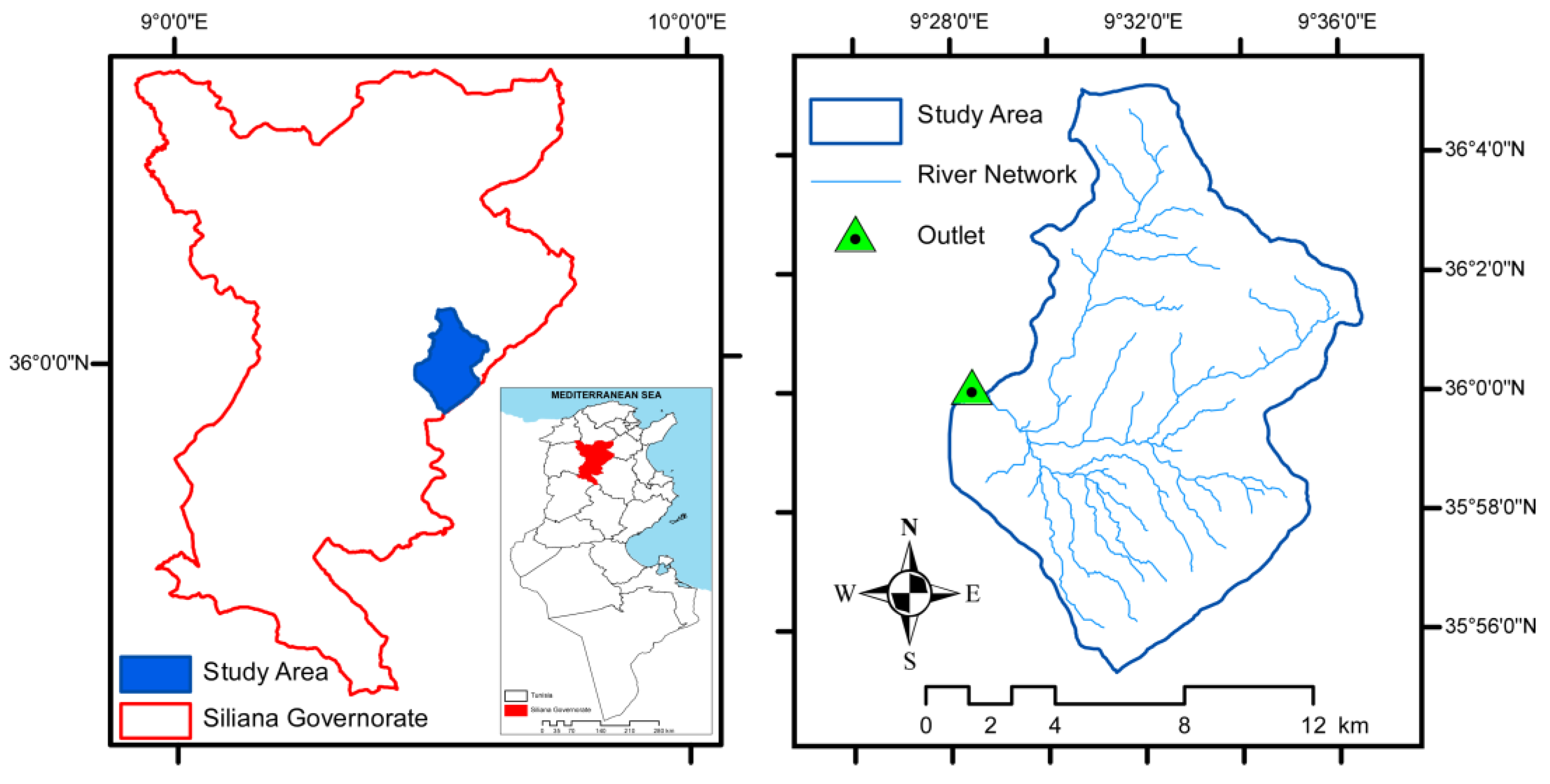
Lakhmass catchment is located in Siliana Governorate, northwestern Tunisia (Figure 1). Lakhmass catchment is a tributary of the Medium Valley of Medjerda, which flows into the Mediterranean Sea [30]. The Northwest, due to its situation and natural characteristics, constitutes the strategic “water table of Tunisia” [30]. Historically, it supplies a large part of the Tunisian population in terms of drinking water and food production, buffering the water deficit of many regions and ensuring sustainable development [31]. The study area is located in the Northern side of the Tunisian Dorsal and is close to the High Tell. Lakhmass catchment (35°59′58″ N, 9°28′31″ E) is a sub-catchment of the Medium Valley of Medjerda and drains an area of 126 km2. It feeds the Lakhmass dam, whose water reservoir, which represents 8% of the total catchment area, is intended for irrigation. The main characteristics of the catchment are summarised in Table 1. Other characteristics are represented in Figure 2.
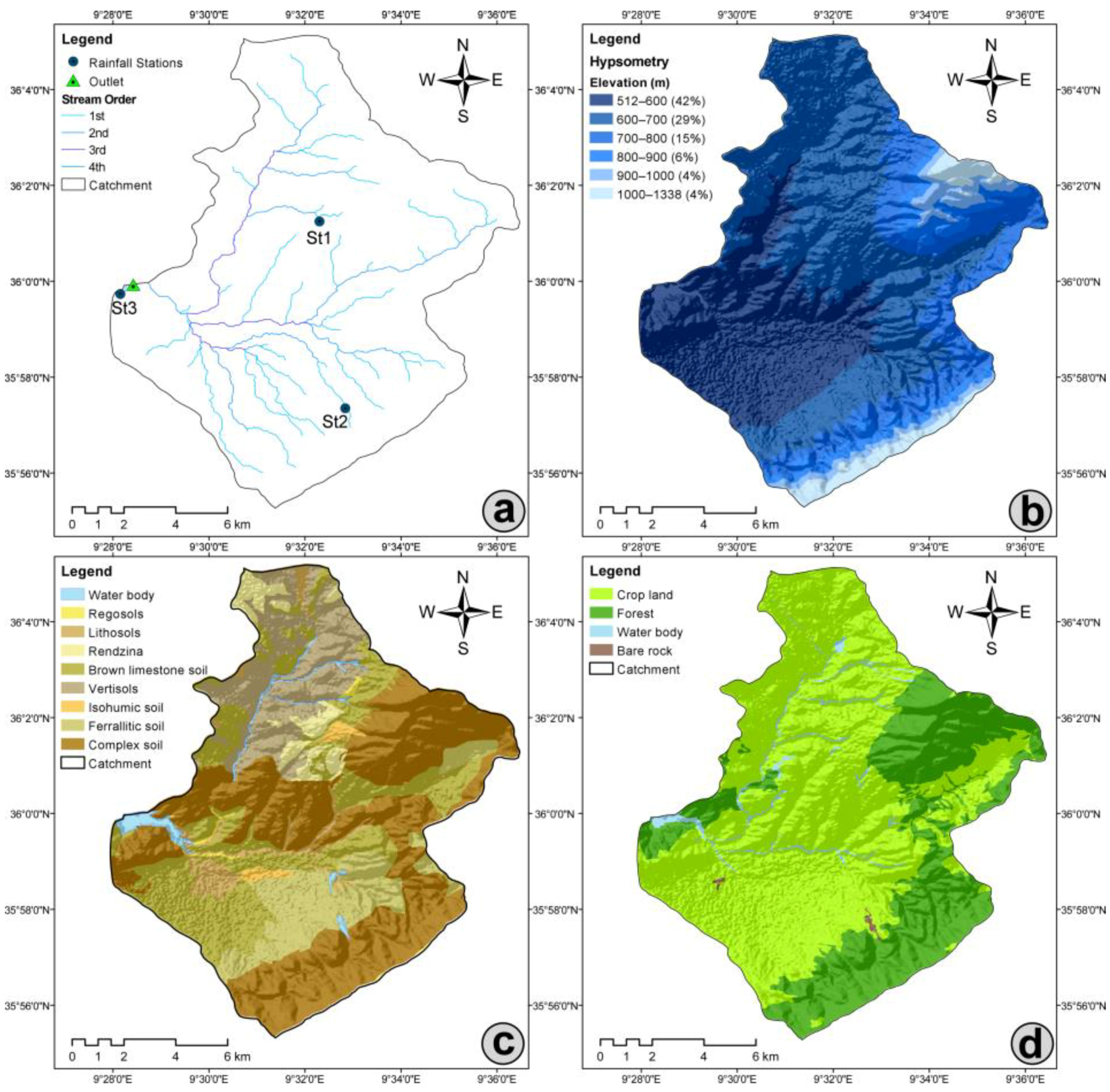
The main wadi supplies the Lakhmass dam with water flow from the heights of two mountains, Djebel Serj and Djebel Bargou. The main river length is 16 km, which originates from Djebel Bargou. According to Strahler classification [32], Lakhmass catchment is drained by a fourth-order stream network (Figure 2a).
Lakmass Catchment is characterised by a varied and rugged relief presenting mountains and valleys [30,31]. A digital elevation model (DEM) shows that the elevation gradually increases from West to East, ranging from 512 m a.s.l. at the Lakhmass dam to 1340 m a.s.l. at Djebel Serj. Djebel Bargou and Djebel Serj bordered the catchment’s eastern and southern parts. The heart of the basin is formed by the vast valley of Ras El Maa. About 42% of the catchment area has an elevation between 512 and 600 m a.s.l., located in the valley upstream of the dam; 29% of the area ranges between 600 and 700 m a.s.l.; and the rest of the area, about 29%, is higher than 700 m a.s.l., near the mountains (Figure 2b).
According to French soil classification, various types of soil exist in Lakhmass catchment (Figure 2c). The main soil class is the complex soil, about 41% of the total area, generally found in the mountain areas and the valley. Brown limestone soil constitutes 22% of the catchment area and deep clayey soil. The vertisols constitute about 15% of the study area, originating from clay material in seasonally humid climates or in areas that are subject to irregular droughts and floods. The rest of the catchment is formed of different types of soil, including ferrallitic soil (11,4%), rendzina (3.8%), regosols (3.7%), stream (1.8%), isohumic soil, and lethosols (1.4%).
In hydrology, land cover plays a crucial role in generating a runoff process on the slopes and the infiltration of rain towards the unsaturated zone. Indeed, the same type of soil may have different behaviours concerning these processes depending on the land use/land cover. Since the early 1970s, with the creation of Lakhmass public irrigated area, agriculture has experienced spectacular development, and the current irrigable area in Siliana covers 15,063 ha [31]. Thus, the main land cover in Lakhmass catchment (Figure 2d) is cropland, with almost 67% of the total area and formed essentially by cereals and fruit trees in the Ras El Maa valley. The forest area corresponds to 31%, mainly located in Djebel Bargou, Djebel Serj and near the Lakhmass dam. The remaining part of the study area is distributed between water bodies and bare ground.
2.2. Data Analysis
The precipitation time-series data were obtained from three different rain stations in Lakhmass catchment (Figure 2a) for 30 years, from 1981 to 2012. The mean total annual precipitation was 452 mm at Lakhmass (524 m a.s.l.), 502 mm at Sidi Hamada (670 m a.s.l.) and 359 mm at Ain Zakkar (667 m a.s.l.), with missing values. The measured annual Potential Evapotranspiration (PET) at Lakhmass meteorological station is 1595–1810 mm, in the period 1981–2014. The temperature data are taken from only one station located in Siliana city, 15 km away from the catchment, with a mean annual air temperature of 18 °C.
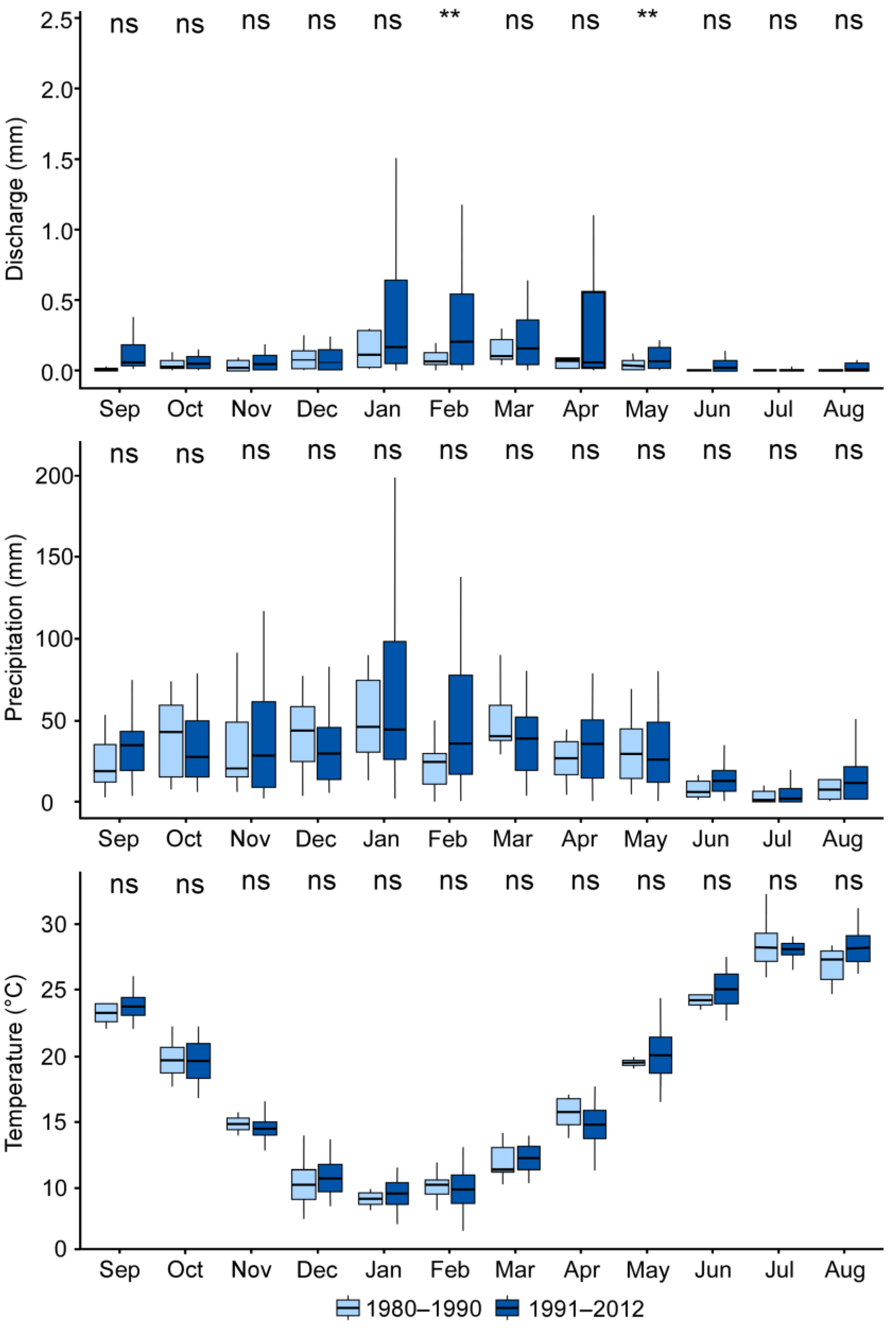
We used a mean comparison test for two periods (the reference period 1980–1990 and the recent period 1991–2012) to investigate data variability at the monthly time step (Figure 3). The box plots of mean monthly precipitation between the two periods show no significant trend, although there is a general increase in precipitation for all months. The median has almost the same value between the two periods, except in the Autumn. The results of a T-test using the rstatix R-package showed that the main changes in precipitation were observed in the extreme values (Q1 (1st quartile), Q3 (3rd quartile), max and min, Figure 3). These results indicate an increase in precipitation variability, impacting catchment hydrology. A general increase, but not significant, in mean temperature is observed (Figure 3). This could be due to the limited period duration.
Generally, discharge tended to increase (comparing the periods 1991–2012 and 1980–1990), but only June and September have a significant increasing trend (Figure 3). The differences are observed in terms of extreme values, especially in the upper quartile (3rd quartile) and maximum values. These results clearly show a perturbation in hydrology due to the introduction of hydro-agriculture management, such as soil and water conservation techniques, in the catchment during the two last decades (1991–2012). The hydrological modeling will not give reasonable results and could not mimic the natural state of the catchment, so this period was excluded in our current investigation. Thus, the model will be used in the reference period (1980–1990), when the catchment hydrology was more natural and was not disturbed by anthropogenic interventions.
2.3. HBV-Light Model and Input Data
The HBV-light model [18] is a hydrological model that does not require a large variety of input data. The HBV-light model has been described in detail elsewhere [33,34,35], hence, only a brief summary is given. The HBV-light model is a conceptual and semi-distributed hydrological model, which was developed by the Swedish Meteorological and Hydrological Institute for the simulation of discharge. In this study, the HBV-light model was employed to simulate and predict discharge at an outlet gauging station of Lakhmass catchment. The main input data were meteorological datasets (precipitation, temperature and evaporation) and hydrological datasets composed of discharge. All input data were given at the daily time step. As the catchment can be subdivided into one or two vegetation zones and lakes, extra data will be implemented (land use, soil type and DEM). Indeed, the model parameters (interception, snow melt and soil moisture capacity) can, however, change according to vegetation type [25]. The model uses the text file format to manage the input/output data. In this study, ArcGIS 10.7 software was used to delineate the catchment and the river network; elaborate hypsometry, soil classes and land-use classes; and extract rainfall station elevations.

Table 2.
Time-series data were used to set up and evaluate the HBV-light model in Lakhmass catchment.
Table 2.
Time-series data were used to set up and evaluate the HBV-light model in Lakhmass catchment.
| Data Type | Data Description | Resolution | Period/Date | Source |
|---|---|---|---|---|
| Meteorological | Air temperature (°C) (1 climate station) | Daily | 1980–2015 | National Institute of Meteorology (INM) |
| Precipitation (mm) (3 rainfall stations) | Daily | 1976–2012 | General Directory of Water Ressources (DGRE) | |
| Hydrological | Discharge (mm) (1 gauging station) | Daily | 1980–2015 (outlet) | General Directory of Dams, Studies and Hydraulic structures (DGBETH) |
| Geographical | Digital Elevation Model (DEM) | 30 m | USGS | |
| Soil type | 1:50,000 | 2002 | Agricultural Map of Siliana (2002) | |
| Land use | 100 m | 2014 | Partnership ESIM-UCLouvain (WBI) [36] |
In the model, the landscape is divided into classes according to soil type, land use and elevation. The model domain can be divided into sub-basins, which can either be independent or connected by rivers and a regional groundwater flow. Each sub-basin can be divided into classes that are the smallest computational spatial unit. Every spatial unit is defined as the hydrological response unit [37]. In the HBV-light model, the common appellations are vegetation and elevation zones [25].
The model calculates the discharge, evapotranspiration, storage and snow melt, soil moisture and fluctuations of groundwater using the adjustment of sixteen parameters distributed in four routines [18]. The snow routine calculates snow melting and accumulation with the adjustment of six parameters (Threshold Temperature (TT), Degree–Day factor (CFmax), seasonal variability in degree-Δt factor (SP), snowfall correction factor (SFCF), refreezing coefficient (CFR), water-holding capacity (CWH)), based on the degree–day factor method [18,33]. The following is the soil moisture routine that simulates actual evapotranspiration, soil moisture and groundwater recharge based on the water storage [35,38]. In this routine, four parameters have to be adjusted (maximum soil moisture (FC), soil moisture threshold for the reduction of evaporation (LP), shape coefficient (BETA) and a correction factor for potential evaporation (CET)) to determine the quantity of water contributing to runoff and the amount that will leave the soil box due to evaporation. As HBV-light is a conceptual model [39], the water process is represented by a set of interconnected reservoirs. The future of the recharge, the soil routine output, is conducted in three boxes where an outflow is released by the control of five parameters (percolation from the upper to lower response box (PERC), threshold parameter for extra outflow from the upper zone (UZL), the additional recession coefficient of the upper groundwater store (K0), the recession coefficient of the upper groundwater store (K1), and the recession coefficient of the lower groundwater store (K2). There is one linear outflow computed from the water level from each box. The routing routine (MAXBAS) follows a transformation function parameter that is characterized by a daily step, representing the base of an equilateral triangular weighting function [18]. The generated runoff of the one-time step is distributed on the following days using this parameter.
As mentioned above, the HBV-light model uses the daily time-series input data of precipitation, temperature and potential evapotranspiration to simulate the daily discharge for a simulation period [18]. The latter is divided into two independent periods for calibration and validation. An extra period is required, which is not taken into consideration for the model performance, called the warming-up period [35].
2.4. Hydrological Model Calibration and Validation
The calibration and the validation of the HBV-light model were conducted using the measured discharge at the gauging station located downstream of Lakhmass dam, the catchment outlet. The simulation period spans from 1981 to 1986, using as input the in-situ data at a daily time step. The periods 1982–1984 and 1984–1986 were used for model calibration and validation, respectively. A manual calibration approach was adopted to simulate the hydrological cycle. It consists of adjusting the model input parameters to the observed discharge with an acceptable fit. The model parameter values were assumed acceptable according to graphical visualization and statistical performance metrics for the calibration and validation periods.
2.5. Model Performance Evaluation
To assess the robustness of the model and to test its fitting accuracy in calibration and validation, we use two statistical metric indexes, Nash and Sutcliffe Efficiency (NSE) and percent bias (PBIAS), as given in Equations (1) and (2):
where Qobs, Qsim and obs are the observed and simulated discharge and the mean of the observed discharge over a time step i of n steps. NSE is a normalised statistic indicator that determines the relative magnitude of the residual variance “noise” of simulated data compared to the measured data variance [40]. The closer the value of NSE is to unity, the higher the correspondence between the simulated and observed hydrographs [40]. The percent bias (PBIAS) measures the average tendency of the simulated values to be larger or smaller than their observed ones [41], which reflects the water-balance error in percent. The optimal value of PBIAS is 0.0, and a negative value indicates an overestimation, and a positive value indicates an underestimation.
2.6. Future Climate Projections
In the context of the EURO-CORDEX initiative (http://www.euro-cordex.net, accessed on 13 September 2021), the European branch of the Coordinated Regional Climate Downscaling Experiment (CORDEX), climate projections are provided using different combinations of General Circulation Models (GCMs) and Regional Climate Models (RCMs) with different grid resolutions [42].
GCMs are used to simulate the response of the global climate system to increasing greenhouse gas concentrations representing physical processes in the atmosphere, ocean, cryosphere and land surface [15]. Different GCMs are available, and, for most of them, their scale is measured in hundreds of kilometers [43]. Usually, their spatial resolution is approximately 100–500 km [43]. RCMs, which are similar to GCMs, simulate the climate for a limited region by being forced with boundary conditions from a global simulation by “downscaling” [15,43]. The scale of an RCM is measured in tens of kilometers in 10–50 km [43].
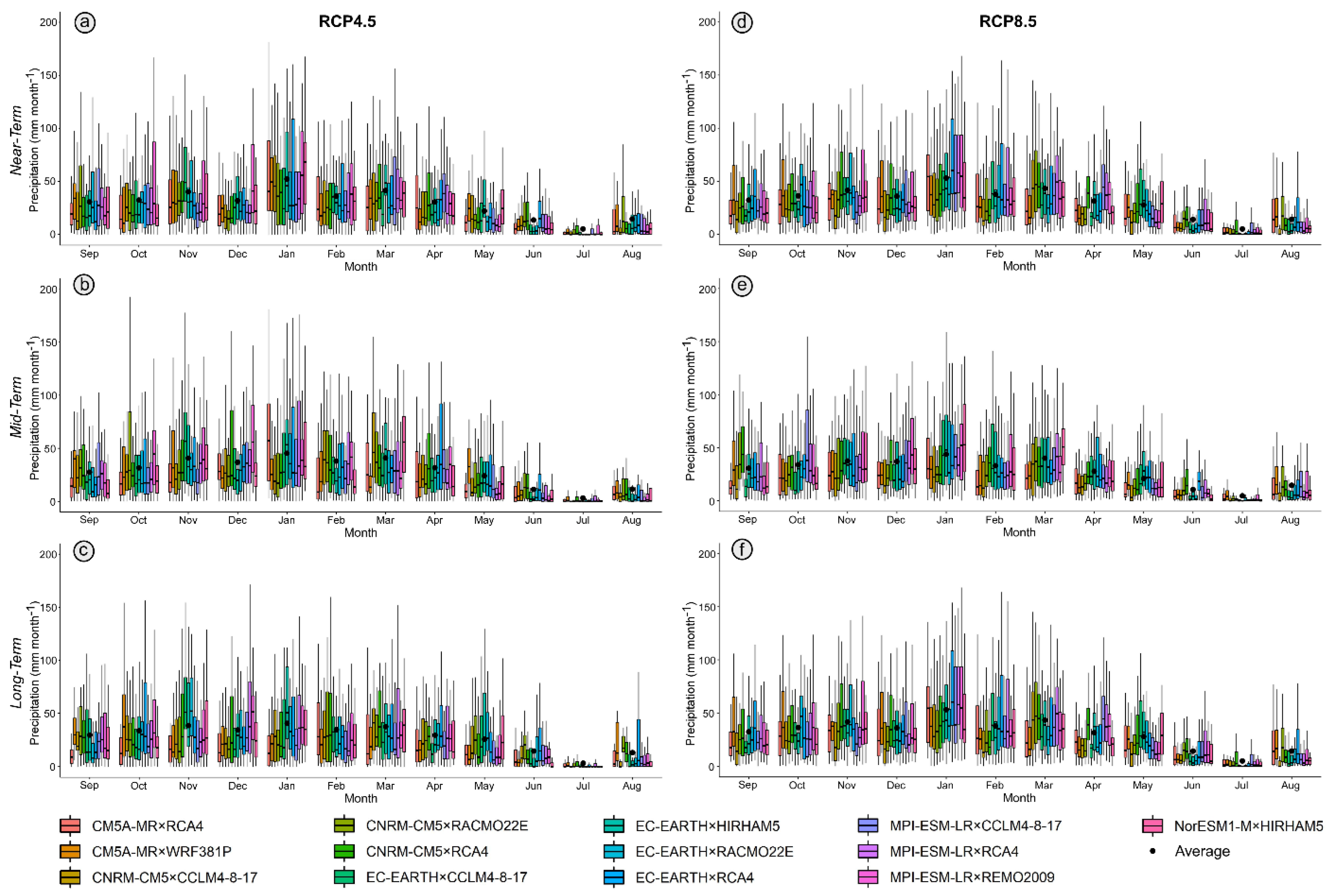
In this work, we made use of the climate models of the EURO-CORDEX initiative with a finer grid resolution of about 12.5 km (EUR-11 grid). To account for the climate model uncertainties, we consider thirteen combinations of climate models (Table 3) composed of five GCMs (CNRM-CM5, NorESM1-M, CM5A-MR, EC-EARTH, MPI-ESM-LR) and six RCMs (CCLM4-8-17, RCA4, HIRHAM5, WRF381P, RACMO22E, REMO2009) based on two RCP scenarios (RCP4.5 and 8.5).
In order to establish climate change scenarios useful for assessing hydrological impacts on a local scale, the raw data of the climate models must be corrected for systematic errors (bias). Of the different methods available in the literature [44], we made use of the distribution mapping method (also known as statistical downscaling). Bias correction was made on a station scale and for each month separately for precipitation and temperature data, based on a control period in which both historical observations and historical climate model projections were simultaneously available. To this aim, one must consider that the available climate model data consist of historical simulations until 2005 and that the scenario runs from 2006 to 2099. To obtain the climate model data at each station, the inverse distance method (power of 2) was adopted, considering the cell that covers the supposed station and its eight neighbouring cells. The downscaling/bias correction was applied to the precipitation and temperature for three rainfall stations (Lakhmass, Sidi Hamada, Ain Zakkar) and Siliana meteorological station.
The precipitation data recorded in 1976–2005 (a 30-year control period) was used to correct the systematic errors (bias correction) in the outputs of the adopted RCMs [23,43] The missing values (gaps) in the recorded precipitation time series for one station were filled through the records available in the best correlated (according to the Pearson correlation coefficient) neighbouring site using linear relationships. According to the RCM ensemble mean and the raw data, the average monthly bias (for the three stations) was in the range [−25, +24] mm, precipitation with values for the single models that reach the range [–118, +39] mm. After bias correction, the maximum monthly differences between observed and simulated values were about ±3 mm. For temperature, the period 1981–2005 (25 years) was chosen to apply the bias correction method. The gaps in the records were filled in two ways: when the missing period was shorter than seven days, a linear variation between the adjacent data was applied. For longer gaps, random values extracted from a normal distribution with a mean and standard deviation of the recorded sample were used. To preserve the seasonality, this method was applied at a monthly scale (i.e., each month of the available selection had its own mean and standard deviation). The average monthly bias before the correction was in the range [+2, +4] °C considering the RCM ensemble mean, with values in the range [−0.1, +7] °C looking at the single RCM models; the bias goes to zero after applying the distribution mapping method.
Daily precipitation and mean daily temperature were given for two RCPs: RCP4.5 and the RCP8.5, suggested by the IPCC AR5. RCP4.5 is a stabilisation pathway in which radiative forcing is limited at approximately 4.5 W·m−2 in the horizon of 2100 [15]. It requires human intervention to reduce GHG emissions under climate-policy socioeconomic reference scenarios [45]. However, the RCP8.5 is defined as a high pathway that leads to radiative forcing higher than 8.5 W·m−2 in 2100 [11] without a climate change policy [46].
The simulation period spans 1 January 1976 to 31 December 2099 for precipitation data and 1 January 1981 to 31 December 2099 for temperature data. To assess future climate change, a historical reference period should be specified to compare climate projections [16]. This reference period is called baseline and spans, in our case, 1981 to 2009. For the analysis of future climate, three periods are used: the near-term period (2010–2039), the mid-term (2040–2069) and the long-term (2070–2099).
3. Results and Discussion
3.1. Model Performance
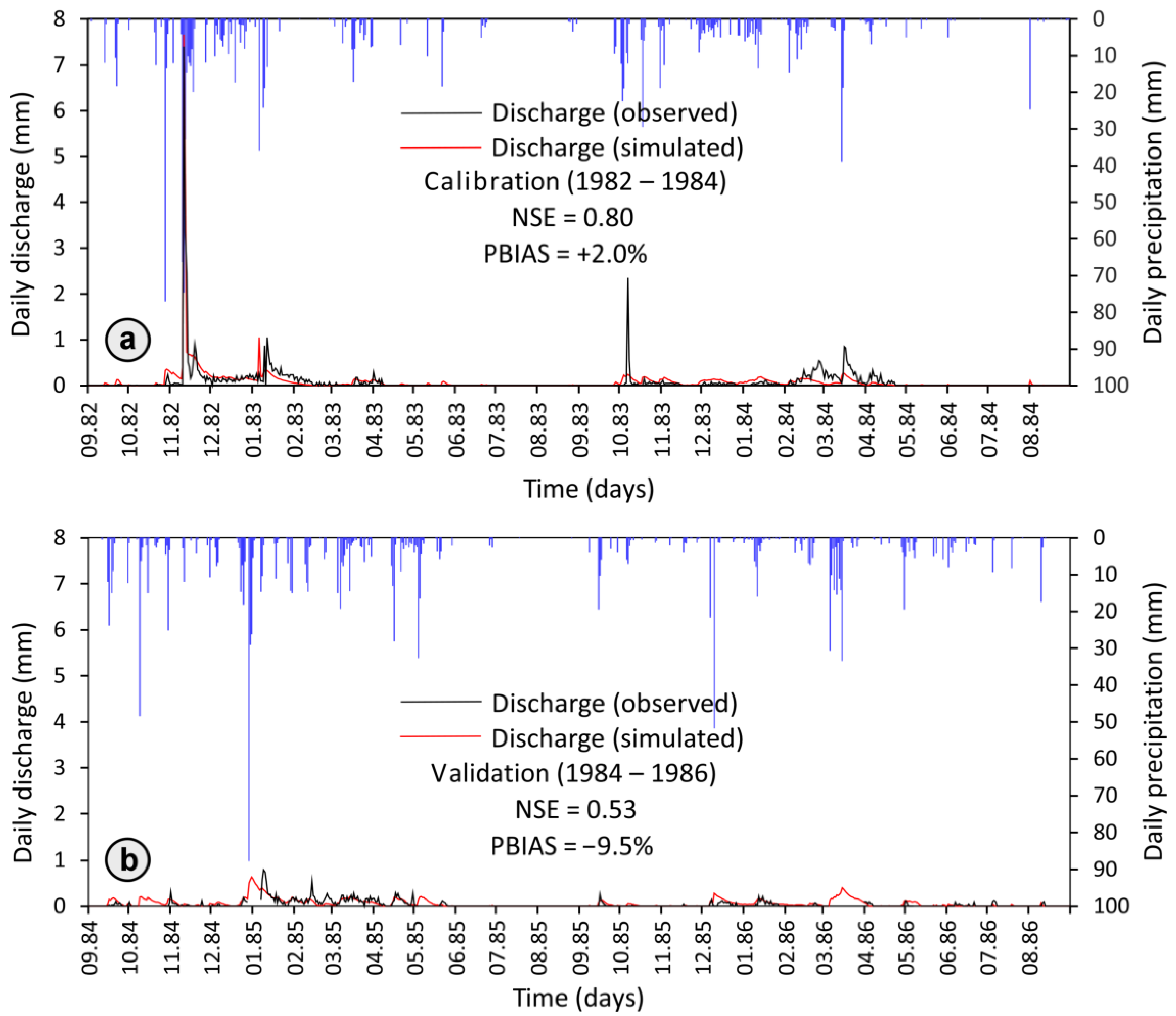
The HBV-light model was calibrated and validated for two-year periods, corresponding to (1982–1984) and (1984–1986), respectively. The model reproduces well the discharge as indicated by the NSE and PBIAS values (Figure 5). Results showed that the model performance is better for the calibration than the validation period, and the NSE value is 0.80 and 0.53, respectively. For the water balance, the PBIAS is better for the calibration period, with +2.0%, than the validation period, with −9.5%. For validation, the HBV-light model overestimates the measured discharge, which is reflected by negative PBIAS values.
3.2. Best-Optimized Model Parameters
The model parameters were calibrated, and their corresponding values are listed in Table 4. The calibration was performed manually by changing the parameters values to get the best fit and the best model performance.
3.3. Effects of Future Climate
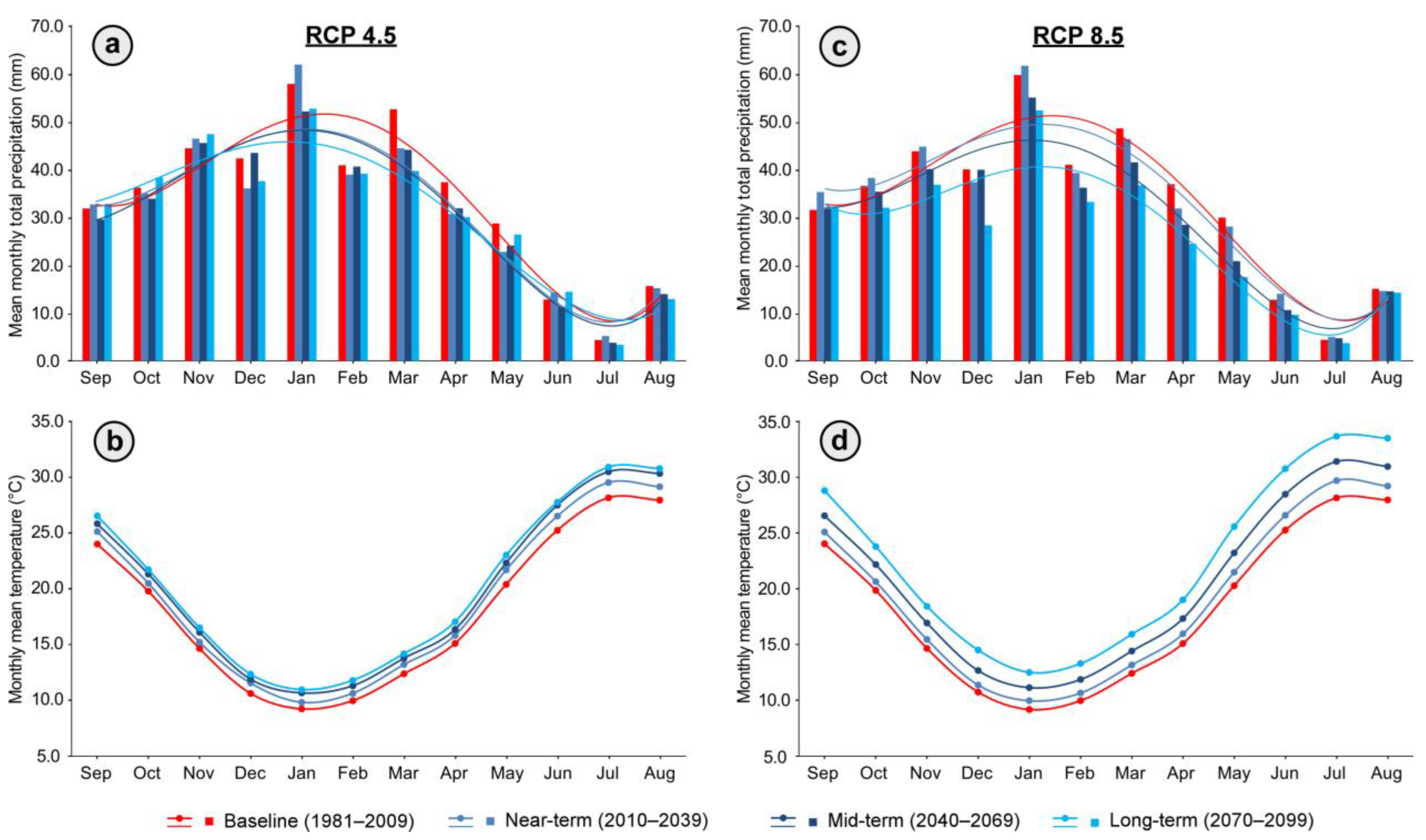
Under the RCP4.5 scenario, the predicted climate data show a general decrease in mean monthly precipitation. In the near-term, precipitation will increase in September, October and January and decrease for the remaining months (Figure 6a). At mid-term, it will generally decrease. For long term, it will only increase in the Autumn and at the beginning of summer (June). In general, mean precipitation will decrease by 5.3, 7.6 and 7.5% in the near-, mid- and long- term, respectively, compared to the baseline period (1981–2009). The temperature will increase by 0.93, 1.70 and 2.17 °C in the near-, mid- and long-term, respectively (Figure 6b). This scenario is based on the introduction of climate change policies, and the hope that greenhouse gas emissions will be reduced by 2050 [15]; a slight change is highlighted between the mid- and the long-term (Figure 6b).
Under RCP8.5, an overall 2.5% increase in precipitation is expected in the near-term period (2010–2039), suggesting that sporadic and intense rains may produce extreme flash floods in the near future. Precipitation will increase from September to January and will decrease from February to May. For the summer, precipitation will remain almost the same (Figure 6c). During the mid-term period (2039–2069), an overall 3% decrease in precipitation is expected for all months. Then, for the long-term period (2070–2099), a steep decline is highlighted in all the months, of about 15% compared to the baseline. Moreover, precipitation in July, August and September will remain almost the same for all terms (Figure 6c). The steadiness may be explained by the increase of extreme weather with high precipitation intensity. The projected temperature shows an increase in mean monthly temperature for all terms of 0.82, 2.25 and 4.00 °C for the near-, mid- and long- term, respectively (Figure 6d). The main changes are highlighted, especially in the summer. These results agree with former studies reporting that, in the Mediterranean, an increase between 3 and 4 °C by 2100 is expected [15].
For both scenarios, the winter is the most affected season by climate change, and we will register less precipitation to reach the lowest precipitation by the end of the century.
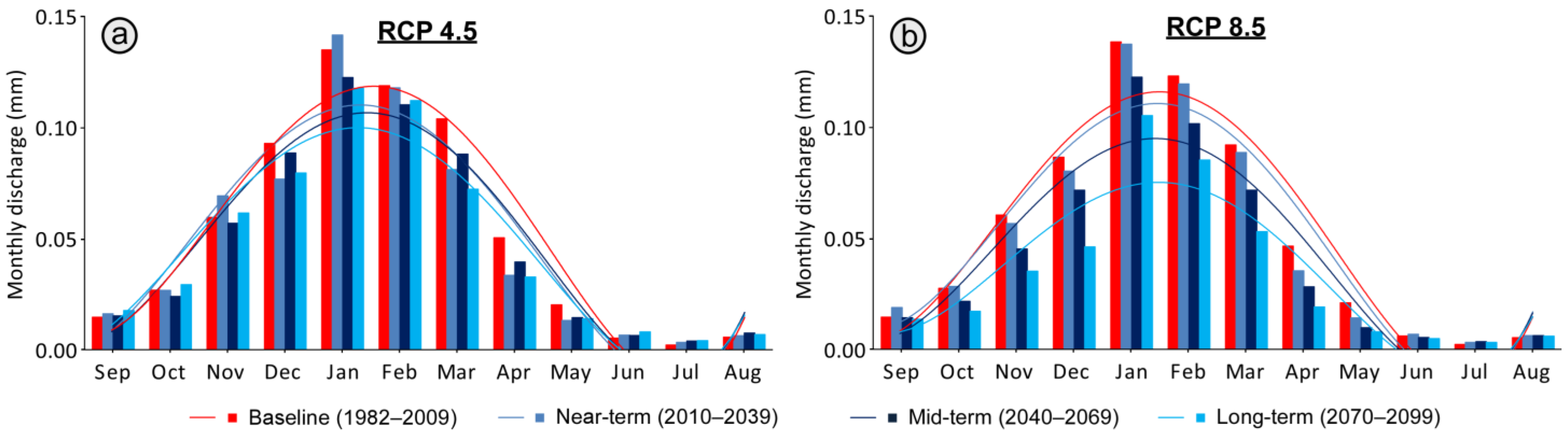
Future climate projections will have a significant effect on the water cycle, especially discharge. The projected discharge was simulated by the HBV-light model using the predicted data of precipitation and temperature under the two scenarios (RCP4.5 and RCP8.5). Generally, discharge tends to decrease (Figure 7). Indeed, it will be reduced by 6.7, 9.1 and 12.5% in the near-, mid-, and long-term, respectively, for RCP4.5 (Figure 7a). For the second scenario, RCP8.5 (Figure 7b), almost 4.6, 19.7 and 36.6% of discharge will be lost by 2040, 2070 and 2100, respectively. The significant decline starts in mid- and long-term periods under RCP8.5 (Figure 7b). Moreover, discharge will decline significantly in the wintertime, which is the season most affected season by climate change.
3.4. Discussion
The model performance during the calibration period is reasonable; however, it degrades during the validation period. The model’s lower performance can be explained by the missing data and the increasing anthropogenic changes, such as small hydraulic infrastructure and land-use changes, on Lakhmass catchment hydrology during the validation period and onwards. These changes could impact the hydrological responses either directly or indirectly through upstream reservoir regulations and the creation, the installation of small hill dams in the catchment and the adaptation of soil and water conservation practices. Missing data and measurement errors (materials, lecture and reporting), which were observed by the quality of the given data time series, could also explain the model’s lower performance during the validation period.
The model was calibrated with very good performance criterion (NSE = 0.80 and PBIAS = +2.0%), according to Kouchi et al.’s classification [46] (i.e., 0.75 < NSE ≤ 1 and PBIAS ≤ ±10%). The performance criteria decreased during validation (NSE = 0.53, PBIAS = −9.5%) but remain satisfactory [47]. For the water balance, the PBIAS is better for the calibration period, with +2.0%, than the validation period, with −9.5%. For validation, the HBV-light model overestimates the measured discharge, which is reflected by negative PBIAS values.
The challenging exercise was calibrating the HBV-light model and using it as a predictive tool to assess the climate change effect on the discharge of Lakhmass catchment. The difficulty originates, essentially, from the availability and quality of the in-situ data (precipitation, temperature and discharge). Since 1985, the catchment has received different hydraulic structures [31] that disturbed discharge and made the catchment less natural compared to the calibration period in late eighties and early nineties of the last century. The chosen calibration period is the more suitable period for a good simulation, as the data series of discharge are less biased. The main reasons behind the variations are reservoir management, soil and water conservation practices, the implementation of small hill dams in the catchment, measurement methods, data collection and uncertainty in data collection. Furthermore, the model performance is affected by the limitations of in-situ data. The precipitation data was taken from only three rainfall stations (Lakhmass, Ain Zakkar and Sidi Hamada) located in the catchment that do not represent the high elevations of Djebel Bargou or Djebel Serj. Moreover, the Ain Zakkar station was not maintained during the observation period, and there are missing data. The temperature data source originates from only one recording station, Siliana station, located 15 km away from the catchment, at a lower elevation. The gaps in the data time series of this station constitute 30% of the total, which will affect the model performance. Furthermore, for the discharge, there is only one gauging station at the outlet of the catchment, and it has numerous gaps. Measured downstream of the catchment through the reservoir level, discharge can be disturbed by reservoir regulations as well as climatic conditions during water level measurement, especially the wind. Gaps during the validation period constitute 10% of the total data. Working with limited data availability and poor quality, we risk the underrepresentation of the basin in its different climatic events and spatial and temporal heterogeneity [8,48].
Indeed, data availability and quality play a key role in modeling performance. The choice of model complexity has a high priority in any study. It should be appropriate to the availability of the data, the purpose of the study and its level of accuracy.
The climate forcing results suggest a severe future climate in Tunisia unless measures are taken or climate policies are established to avoid at least the second scenario, RCP8.5, in particular because climate change will affect Mediterranean countries more than other regions [12]. According to IPCC-AR5 [15], the temperature will increase in the Mediterranean region by 2 to 3 °C by 2050 and 3 to 5 °C by 2100. For Lakhmass catchment case study, the climate data (2010–2099) predict an increase of temperature by almost 2.17 °C and 4 °C by 2100 under RCP4.5 and RCP8.5, respectively. This increase seems to be accompanied by a decrease in annual precipitation of 7.5 and 15%, by 2100, under RCP4.5 and RCP8.5, respectively. However, precipitation is not projected to continuously decrease. An increase in projected precipitation will be expected from term to term due to the increased intensity and frequency of extreme hydrologic and weather events. Previous papers in the Mediterranean region predicted a decline in precipitation by 4% for every degree of global warming [2,16].
Furthermore, studies affirm that precipitation will decrease under climate change significantly for the wintertime [8,13], which is clearly confirmed by our results for both scenarios. Climate change will have an effect on the discharge of Lakhmass catchment, which is predicted to decrease by 12.5% and 36.6% in RCP4.5 and RCP8.5, respectively, by 2100. For both scenarios, no significant changes are highlighted between the near-term and the baseline. However, from the mid-term, we conclude that discharge will decrease dramatically.
4. Conclusions
Being part of the Mediterranean region with a semi-arid climate, Lakhmass catchment (126 km²) has significant variability in precipitation and temperature. Furthermore, the catchment received multiple anthropogenic interventions (soil and water conservation practices, the creation of small hill dams), which disturbed its hydrology and its natural responsiveness but generally remain statistically non-significant. To reconstruct its hydrology, the HBV-light model was calibrated and validated with acceptable performance criteria for the periods 1982–1984 and 1984–1986, respectively. To simulate future discharge, we analyzed the projected climate data given from thirteen climate models of the EURO-CORDEX initiative, under RCP4.5 and RCP8.5. The provided data series served as input to the HBV-light model to simulate the future discharge at three projections periods: near-term (2010–2039), mid-term (2040–2069) and long-term (2070–2099). The results showed that, by the long-term horizon, an increase in temperature of 2.7 °C and 4 °C under RCP4.5 and RCP8.5 is accompanied with a decrease of almost 5% of precipitation for every +1 °C of expected global warming. These changes will significantly affect the hydrological cycle and response of Lakhmass catchment. Thus, the discharge will be reduced by 12.5% and 36.6% under RCP4.5 and RCP8.5, respectively.
This study revealed that the setup of a hydrological model as a scientific and decision-making tool for investigating the impacts of climate change in a semi-arid region known for its data scarcity and complex hydrology requires a careful selection of the calibration period. Therefore, training the hydrological model in natural conditions with less perturbated situations is crucial to ensure reasonable model parameter estimation during a reference period assumed as baseline conditions. In addition, the future climate projections should be conducted carefully in the Mediterranean context compared to other regions, as it is considered a climate change hotspot and an outlier of global warming. Thus, combining thirteen climate models with bias correction was essential to considering regional climate projection uncertainty under two RCP scenarios. This investigation also showed that a good balance between in-situ data availability, model complexity and data requirements is important to match reasonable hydrological prediction and avoid model over-parameterization.
Author Contributions
Study design and organization, S.B.N., S.J. and S.K.; data collection and GIS analysis, S.B.N., S.K., S.J. and Ü.Y.; HBV-light model setup and running, S.B.N., S.J., M.R., X.Z. and S.K.; climate analysis and scenarios, M.D.; discussion of results, writing and review manuscript, All authors. All authors have read and agreed to the published version of the manuscript.
Funding
This research received no external funding.
Institutional Review Board Statement
Not applicable.
Informed Consent Statement
Not applicable.
Data Availability Statement
The hydrological input data used for the HBV-light model simulations presented in this study are available upon request from the author Slaheddine Khlifi. The original time series of discharge were given by the DGBETH whereas rain data collected by DGRE in Tunisia. For the climate forcing data bias correction, daily temperature observations were obtained from INM and precipitation data from DGRE. All data series are not publicly available due to the restrictions of DGRE and INM, and data should be provided upon specific request.
Acknowledgments
The data sets utilized in this study in part originated from the Master’s dissertation of the author Siwar Ben Nsir, which was supported by the Higher School of Engineers of Medjez El Bab, University of Jendouba in Tunisia, under the supervision of Slaheddine Khlifi and Seifeddine Jomaa. The authors would also like to acknowledge the scholarship provided by the Ministry of High Education and Scientific Research to the author Siwar Ben Nsir for her internship at UFZ. We used the R programing language for the analysis of climate data.
Conflicts of Interest
The authors declare no conflict of interest.
References
- Tsanis, I.K.; Koutroulis, A.G.; Daliakopoulos, I.N.; Jacob, D. Severe climate-induced water shortage and extremes in Crete. Clim. Chang. 2011, 106, 667–677. [Google Scholar] [CrossRef]
- Lionello, P.; Scarascia, L. The relation between climate change in the Mediterranean region and global warming. Reg. Environ. Chang. 2018, 18, 1481–1493. [Google Scholar] [CrossRef]
- Cramer, W.; Guiot, J.; Fader, M.; Garrabou, J.; Gattuso, J.P.; Iglesias, A.; Lange, M.A.; Lionello, P.; Llasat, M.C.; Paz, S.; et al. Climate change and interconnected risks to sustaina-ble development in the Mediterranean. Nat. Clim. Chang. 2018, 8, 972–980. [Google Scholar] [CrossRef] [Green Version]
- United Nations Environment Programme. Adaptation Gap Report 2020; UNEP: Nairobi, Kenya, 2021. [Google Scholar]
- Immerzeel, W.W.; Lutz, A.F.; Andrade, M.; Bahl, A.; Biemans, H.; Bolch, T.; Hyde, S.; Brumby, S.; Davies, B.J.; Elmore, A.C.; et al. Importance and vulnerability of the world’s water towers. Nature 2020, 577, 364–369. [Google Scholar] [CrossRef]
- United Nations Environment Programme. Making Peace with Nature: A Scientific Blueprint to Tackle the Climate, Biodiversity and Pollution Emergencies; UNEP: Nairobi, Kenya, 2021. [Google Scholar]
- Radoslav, S.D. The Paris Agreement on Climate Change: Behind Closed Doors. Glob. Environ. Polit. 2016, 16, 1–11. [Google Scholar]
- United Nations. Paris Agreement; United Nations: Paris, France, 2015. [Google Scholar]
- Yıldırım, Ü.; Güler, C.; Önol, B.; Rode, M.; Jomaa, S. Modelling of the Discharge Response to Climate Change un-der RCP8.5 Scenario in the Alata River Basin (Mersin, SE Turkey). Water 2021, 13, 483. [Google Scholar] [CrossRef]
- Lembaid, I.; Moussadek, R.; Mrabet, R.; Bouhaouss, A. Modeling Soil Organic Carbon Changes under Alternative Climatic Scenarios and Soil Properties Using DNDC Model at a Semi-Arid Mediterranean Environment. Climate 2022, 10, 23. [Google Scholar] [CrossRef]
- Rizzo, A.; Vandelli, V.; Gauci, C.; Buhagiar, G.; Micallef, A.S.; Soldati, M. Potential Sea Level Rise Inundation in the Mediterranean: From Susceptibility Assessment to Risk Scenarios for Policy Action. Water 2022, 14, 416. [Google Scholar] [CrossRef]
- Pulighe, G.; Lupia, F.; Chen, H.; Yin, H. Modeling Climate Change Impacts on Water Balance of a Mediterranean Watershed Using SWAT+. Hydrology 2021, 8, 157. [Google Scholar] [CrossRef]
- United Nations Environment Programme. State of the Environment and Development in the Mediterranean (SoED). Plan Bleu 2019. Available online: https://planbleu.org/soed/ (accessed on 20 September 2021).
- Tuel, A.; Eltahir, E.A.B. Why is the Mediterranean a Climate Change Hot Spot? J. Clim. 2020, 33, 5829–5843. [Google Scholar] [CrossRef]
- Allen, M.R.; Dube, O.P.; Solecki, W.; Aragón-Durand, F.; Cramer, W.; Humphreys, S.; Kainuma, M.; Kala, J.; Mahowald, N.; Mulugetta, Y.; et al. Framing and Context. In Global Warming of 1.5 °C. An IPCC Special Report on the Impacts of global warming of 1.5°C above Pre-Industrial Levels and Related Global Greenhouse Gas Emission Pathways, in the Context of Strengthening the Global Response to the Threat of Climate Change, Sustainable Development, and Efforts to Eradicate Poverty; Masson-Delmotte, V., Zhai, P., Pörtner, H.-O., Roberts, D., Skea, J., Shukla, P.R., Pirani, A., Moufouma-Okia, W., Péan, C., Pidcock, R., et al., Eds.; Cambridge University Press: Cambridge, UK; New York, NY, USA, 2018; p. 49. Available online: https://www.ipcc.ch/sr15/chapter/chapter-1/ (accessed on 17 August 2021).
- MedCC. Climate and Environmental Change in the Mediterranean Basin—Current Situation and Risks for the Future. First Mediterranean Assessment Report (MAR1); Cramer, W., Guiot, J., Marini, K., Eds.; Plan Bleu, UNEP/MAP: Marseille, France, 2020. [Google Scholar]
- Reinecke, R.; Müller Schmied, H.; Trautmann, T.; Andersen, L.S.; Burek, P.; Flörke, M.; Gosling, S.N.; Grillakis, M.; Hanasaki, N.; Koutroulis, A.; et al. Uncertainty of simulated groundwater recharge at different global warming levels: A global-scale multi-model ensemble study. Hydrol. Earth Syst. Sci 2021, 25, 787–810. [Google Scholar] [CrossRef]
- Seibert, J.; Vis, M.J.P. Teaching hydrological modeling with a user-friendly catchment-runoff-model software package. Hydrol. Earth Syst. Sci. 2012, 16, 3315–3325. [Google Scholar] [CrossRef] [Green Version]
- Engel, B.; Storm, D.; White, M.; Arnold, J.; Arabi, M. A Hydrologic/Water Quality Model Application Protocol. J. Am. Water Resour. Assoc. 2007, 43, 1223–1236. [Google Scholar] [CrossRef]
- Chaibou Begou, J.; Jomaa, S.; Benabdallah, S.; Bazie, P.; Afouda, A.; Rode, M. Multi-Site Validation of the SWAT-Model on the Bani Catchment: Model Performance and Predictive Uncertainty. Water 2016, 8, 178. [Google Scholar] [CrossRef]
- Chen, J.; Gao, C.; Zeng, X.; Xiong, M.; Wang, Y.; Jing, C.; Krysanova, V.; Huang, H.; Zhao, N.; Su, B. Assessing changes of river discharge under global warming of 1.5 °C and 2 °C in the upper reaches of the Yangtze River Basin: Approach by using multiple- GCMs and hydrological models. Quat. Int. 2017, 453, 63–73. [Google Scholar] [CrossRef]
- Moss, R.H.; Edmonds, J.A.; Hibbard, K.A.; Manning, M.R.; Rose, S.K.; Van Vuuren, D.P.; Wilbanks, T.J. The next generation of scenarios for climate change research and assessment. Nature 2010, 463, 747–756. [Google Scholar] [CrossRef]
- Dakhlaoui, H.; Djebbi, K. Evaluating the impact of rainfall–runoff model structural uncertainty on the hydrological rating of regional climate model simulations. J. Water Clim. Chang. 2021, 12, 3820–3838. [Google Scholar] [CrossRef]
- Boulmaiz, T.; Boutaghane, H.; Abida, H.; Saber, M.; Kantoush, S.A.; Tramblay, Y. Exploring the Spatio-Temporal Variability of Precipitation over the Medjerda Transboundary Basin in North Africa. Water 2022, 14, 423. [Google Scholar] [CrossRef]
- Bergström, S. Development and Application of a Conceptual Runoff Model for Scandinavian Catchments; Reports Hydrolgy 7; Swedish Meteorological and Hydrological Institute (SMHI): Norrköping, Sweden, 1976. [Google Scholar]
- Bergström, S. The HBV Model—Its Structure and Applications; Reports Hydrolgy 4; Swedish Meteorological and Hydrological Institute (SMHI): Norrköping, Sweden, 1992. [Google Scholar]
- M’chirgui, R.; Bargaoui, Z.; Bardossy, A. Incidence de l’incertitude pluviométrique sur la modélisation pluie-débit. In Soil-Vegetation-Atmosphere Transfer Schemes and Large-Scale Hydrological Models, Proceedings of the a Symposium Held during the Sixth IAHS Scientific Assembly, Maastricht, The Netherlands, 18–27 July 2001; IAHS: Oxfordshire, UK, 2001. [Google Scholar]
- Ouachani, R.; Bargaoui, Z.; Ouarda, T. Intégration d’un filtre de Kalman dans le modèle hydrologique HBV pour la prévision des débits. Hydrol. Sci. J. 2007, 52, 318–337. [Google Scholar] [CrossRef] [Green Version]
- Dakhlaoui, H.; Ruelland, D.; Tramblay, Y.; Bargaoui, Z. Evaluating the robustness of conceptual rainfall-runoff models under climate variability in northern Tunisia. J. Hydrol. 2017, 550, 201–217. [Google Scholar] [CrossRef]
- MEHAT. Schéma Directeur d’Amenagement de la Région Economique du Nord-Ouest; Ministère de l’Equipement de l’Habitat et de l’Amengament du Territoire: Tunis, Tunisia, 2010. [Google Scholar]
- MEHAT. Atlas du Gouvernorat de Siliana; Ministère de l’Equipement de l’Habitat et de l’Amengament du Territoire: Tunis, Tunisia, 2013. [Google Scholar]
- Strahler, A.N. Quantitative analysis of watershed geomorphology. Eos Trans. Am. Geophys. Union 1957, 38, 913–920. [Google Scholar] [CrossRef] [Green Version]
- Bergström, S. The HBV model. In Computer Models of Watershed Hydrology; Singh, V.P., Ed.; Water Resources Publications: Highlands Ranch, CO, USA, 1995; Chapter 13; pp. 443–476. [Google Scholar]
- Lindström, G.; Johansson, B.; Persson, M.; Gardelin, M.; Bergström, S. Development and test of the distributed HBV-96 hydrological model. J. Hydrol. 1997, 201, 272–288. [Google Scholar] [CrossRef]
- Seibert, J. Regionalisation of parameters for a conceptual rainfall-runoff model. Agric. For. Meteorol. 1999, 98–99, 279–293. [Google Scholar] [CrossRef]
- Sellami, H.; Vanclooster, M.; Khlifi, S.; Gara, A.; Mahjoub, M.R. Gestion des ressources en eau dans la Medjerda: Modélisation hydrologique. In Proceedings of the Renforcement de la Formation Supérieure et de la Recherche en Gestion Intégrée des Ressources en eau de la Medjerda, Medjez El Bab, Tunisia, 20 November 2014. [Google Scholar]
- Flügel, W.A. Delineating hydrological response units by geographical information system analyses for regional hydro-logical modelling using PRMS/MMS in the drainage basin of the River Bröl, Germany. Hydrol. Process. 1995, 9, 423–436. [Google Scholar] [CrossRef]
- Seibert, J. Estimation of parameter uncertainty in the HBV model. Hydrol. Res. 1997, 28, 247–262. [Google Scholar] [CrossRef]
- Bergestrôm, S.; Forsman, A. Development of a conceptual deterministic rainfall-runoff model. Hydrol. Res. 1973, 4, 147–170. [Google Scholar] [CrossRef]
- Nash, J.E.; Sutcliffe, J.V. River flow forecasting through conceptual models part I—A discussion of principles. J. Hydrol. 1970, 10, 282–290. [Google Scholar] [CrossRef]
- Yen, H.; Hoque, Y.; Harmel, R.D.; Jeong, J. The impact of considering uncertainty in measured calibration/validation data during auto-calibration of hydrologic and water quality models. Stoch. Environ. Res. Risk Assess. 2015, 29, 1891–1901. [Google Scholar] [CrossRef]
- Jacob, D.; Petersen, J.; Eggert, B.; Alias, A.; Christensen, O.B.; Bouwer, L.M.; Yiou, P. EURO-CORDEX: New high-resolution climate change projections for European impact research. Reg. Environ. Chang. 2013, 14, 563–578. [Google Scholar] [CrossRef]
- D’Oria, M.; Ferraresi, M.; Tanda, M.G. Historical trends and high-resolution future climate projections in northern Tuscany (Italy). J. Hydrol. 2017, 555, 708–723. [Google Scholar] [CrossRef]
- Teutschbein, C.; Seibert, J. Bias correction of regional climate model simulations for hydrological climate-change impact studies: Review and evaluation of different methods. J. Hydrol. 2012, 456–457, 12–29. [Google Scholar] [CrossRef]
- Thomson, A.M.; Calvin, K.V.; Smith, S.J.; Kyle, G.P.; Volke, A.; Patel, P.; Delgado-Arias, S.; Bond-Lamberty, B.; Wise, M.A.; Clarke, L.E.; et al. RCP4.5: A pathway for stabilization of radiative forcing by 2100. Clim. Chang. 2011, 109, 77–94. [Google Scholar] [CrossRef] [Green Version]
- Riahi, K.; Rao, S.; Krey, V.; Cho, C.; Chirkov, V.; Fischer, G.; Kindermann, G.; Nakicenovic, N.; Rafaj, P. RCP 8.5—A scenario of comparatively high greenhouse gas emissions. Clim. Chang. 2011, 109, 33–57. [Google Scholar] [CrossRef] [Green Version]
- Kouchi, D.H.; Esmaili, K.; Faridhosseini, A.; Sanaeinejad, S.H.; Khalili, D.; Abbaspour, K.C. Sensitivity of Calibrated Parameters and Water Resource Estimates on Different Objective Functions and Optimization Algorithms. Water 2017, 9, 384. [Google Scholar] [CrossRef] [Green Version]
- Jiang, S.; Jomaa, S.; Büttner, O.; Meon, G.; Rode, M. Multi-site identification of a distributed hydrological nitrogen model using Bayesian uncertainty analysis. J. Hydrol. 2015, 529, 940–950. [Google Scholar] [CrossRef]
Figure 1.
Lakhmass catchment location, river network and outlet gauging station.

Figure 2.
Maps showing the (a) Strahler’s order and rain stations (St1: Ain Zakkar, St2: Sidi Hamada and St3: Lakhmass, with annual mean total precipitation values of 359 mm, 502 mm and 452 mm, and elevations of 667 m a.s.l., 670 m a.s.l. and 534 m a.s.l., respectively), (b) hypsometry, (c) soil classes and (d) land-use classes of Lakhmass catchment. Precipitation data were collected from the Tunisian General Directory of Water Resources (DGRE).

Figure 3.
Box plots of mean monthly discharge, precipitation and temperature of the reference and the recent periods at Lakhmass catchment. ns means no significant changes (p value > 0.05) between the two investigation periods, while ** indicates that there is a statistically significant change (p value ≤ 0.01).

Figure 4.
Box plots of mean monthly precipitation projections derived from thirteen climate models (a) in the near-term, (b) the mid-term and (c) the long-term under RCP4.5 and (d) in the near-term, (e) the mid-term and (f) the long-term under RCP8.5.
Figure 4.
Box plots of mean monthly precipitation projections derived from thirteen climate models (a) in the near-term, (b) the mid-term and (c) the long-term under RCP4.5 and (d) in the near-term, (e) the mid-term and (f) the long-term under RCP8.5.

Figure 5.
Observed and predicted discharge at daily time steps during (a) calibration (1982–1984) and (b) validation (1984–1986) at the outlet of Lakhmass catchment.
Figure 5.
Observed and predicted discharge at daily time steps during (a) calibration (1982–1984) and (b) validation (1984–1986) at the outlet of Lakhmass catchment.

Figure 6.
Variation of monthly precipitation (a), monthly temperature (b) under RCP4.5, monthly precipitation (c) and monthly temperature (d) under RCP8.5 for the baseline, near-, mid- and long-term at Lakhmass catchment. Trend lines using a polynomial fitting curve with 4th order were added for each period of monthly precipitation.

Figure 7.
Monthly discharge under RCP4.5 (a) and monthly discharge under RCP8.5 (b) for the baseline, near-term, mid-term and long-term at Lakhmass catchment. Trend lines using a polynomial fitting curve with 4th order were added for each period.
Figure 7.
Monthly discharge under RCP4.5 (a) and monthly discharge under RCP8.5 (b) for the baseline, near-term, mid-term and long-term at Lakhmass catchment. Trend lines using a polynomial fitting curve with 4th order were added for each period.

Table 1.
Basic characteristics of Lakhmass catchment, in Siliana, Northwest Tunisia. Note that the data sources used to derive the basic characteristics of Lakhmass catchment are presented in Table 2. a The Thiessen polygon method was used to calculate precipitation spatially.
Table 1.
Basic characteristics of Lakhmass catchment, in Siliana, Northwest Tunisia. Note that the data sources used to derive the basic characteristics of Lakhmass catchment are presented in Table 2. a The Thiessen polygon method was used to calculate precipitation spatially.
| Characteristic | Unit | Value | Characteristic | Unit | Value |
|---|---|---|---|---|---|
| Catchment area | km2 | 126 | Soil type | ||
| Strahler’s stream order | – | 4 | Complex soil | % | 41 |
| Hydrology (1981–2012) | Brown limestone soil | % | 22 | ||
| Discharge at the outlet (daily mean) | m3/s | 2.99 | Vertisols | % | 15 |
| Precipitation (mean) a | mm/y | 452 | Ferralitic soil | % | 11.4 |
| Temperature (mean) | °C | 18 | Rendzina | % | 3.8 |
| Elevation range (m) | Lithosols | % | 3.7 | ||
| 512–600 | % | 42 | Waterbody | % | 1.8 |
| 600–700 | % | 29 | Isohumic soil and Regosols | % | 1.4 |
| 700–800 | % | 15 | Land use (in 2014) | ||
| 800–900 | % | 6 | Cropland | % | 67 |
| 900–1000 | % | 4 | Forest | % | 31 |
| 1000–1338 | % | 4 |
Table 3.
Climate models combinations: five GCMs and six RCMs for precipitation and temperature projections.
Table 3.
Climate models combinations: five GCMs and six RCMs for precipitation and temperature projections.
| GCMs | CNRM-CM5 | NorESM1-M | CM5A-MR | EC-EARTH | MPI-ESM-LR | |
| RCMs | ||||||
| CCLM4-8-17 | X | X | X | |||
| RCA4 | X | X | X | X | ||
| HIRHAM5 | X | X | ||||
| WRF381P | X | |||||
| RACMO22E | X | X | ||||
| REMO2009 | X | |||||
Table 4.
HBV-light model’s optimised parameters obtained from calibration for Lakhmass catchment.
| Parameter | Physical Meaning | Vegetation Zone 1 | Vegetation Zone 2 |
|---|---|---|---|
| Snow Routine | |||
| TT (°C) | Temperature threshold of evaporation and snow accumulation | 2 | 2 |
| CFmax (mm/°C/day) | Degree–day factor | 1.5 | 1.5 |
| SP | Seasonal variability | 0 | 0 |
| SFCF (–) | Snowfall correction factor | 0.01 | 0.01 |
| CFR (–) | Refreezing coefficient | 0.05 | 0.05 |
| CWH (–) | Water-holding capacity | 0.1 | 0.1 |
| Soil Moisture Routine | |||
| FC (mm) | Field capacity (maximum soil moisture storage) | 190 | 450 |
| LP (mm) | Limiting factor of soil moisture above which AET reaches PET | 0.01 | 0.01 |
| BETA (–) | Shape parameter: contribution to runoff from rain or snowmelt | 5.3 | 4.8 |
| Response Routine | |||
| PERC (mm) | Threshold parameter | 0.07 | |
| UZL (mm) | Limit of soil box that generate discharge | 20 | |
| K0 (day−1) | Recession coefficient (peak part) | 0.6 | |
| K1 (day−1) | Recession coefficient (intermediate part) | 10-6 | |
| K2 (day−1) | Recession coefficient (baseflow part) | 0.1 | |
| Routing Routine | |||
| MAXBAS (day) | Time constant of the unit hydrograph | 1 | |
| CET (°C−1) | Potential evaporation correction factor | 0.09 | |
Publisher’s Note: MDPI stays neutral with regard to jurisdictional claims in published maps and institutional affiliations. |
© 2022 by the authors. Licensee MDPI, Basel, Switzerland. This article is an open access article distributed under the terms and conditions of the Creative Commons Attribution (CC BY) license (https://creativecommons.org/licenses/by/4.0/).
Share and Cite
MDPI and ACS Style
Ben Nsir, S.; Jomaa, S.; Yıldırım, Ü.; Zhou, X.; D’Oria, M.; Rode, M.; Khlifi, S. Assessment of Climate Change Impact on Discharge of the Lakhmass Catchment (Northwest Tunisia). Water 2022, 14, 2242. https://doi.org/10.3390/w14142242
AMA Style
Ben Nsir S, Jomaa S, Yıldırım Ü, Zhou X, D’Oria M, Rode M, Khlifi S. Assessment of Climate Change Impact on Discharge of the Lakhmass Catchment (Northwest Tunisia). Water. 2022; 14(14):2242. https://doi.org/10.3390/w14142242
Chicago/Turabian StyleBen Nsir, Siwar, Seifeddine Jomaa, Ümit Yıldırım, Xiangqian Zhou, Marco D’Oria, Michael Rode, and Slaheddine Khlifi. 2022. "Assessment of Climate Change Impact on Discharge of the Lakhmass Catchment (Northwest Tunisia)" Water 14, no. 14: 2242. https://doi.org/10.3390/w14142242
Note that from the first issue of 2016, this journal uses article numbers instead of page numbers. See further details here.