
Relationships between Fish Communities and Habitat before and after a Typhoon Season in Tropical Mountain Streams


1
Department of Ecology and Environmental Resources, National University of Tainan, 33, Section 2, Shu-Lin St., Tainan 70005, Taiwan
2
International Joint Commission, Great Lakes Office, P.O. Box 32869, Detroit, MI 48232, USA
3
No. 67, Aly. 3, Ln. 362, Sec. 1, Chunghwa North Rd., Tainan 70459, Taiwan
*
Author to whom correspondence should be addressed.
Water 2022, 14(14), 2220; https://doi.org/10.3390/w14142220
Submission received: 1 June 2022
/
Revised: 11 July 2022
/
Accepted: 13 July 2022
/
Published: 14 July 2022
(This article belongs to the Section Biodiversity and Functionality of Aquatic Ecosystems)
Abstract
:The responses of habitat and fish communities to extreme hydrological and habitat disturbance in typhoon-prone mountain streams are not studied much. Such landscape–climate settings may provide a unique opportunity for fish to evolve without special habitat adaptation and involve different assembly rules compared to temperate regions. This study aimed to compare fish communities and habitat factors before and after the typhoon season and to test the influences of various aspects of habitat on fish assemblages between seasons. Fish and habitats were surveyed at 30 wadable stream sites in March and December 2010 in tropical southern Taiwan. Habitat variables differed between the pre-typhoon and post-typhoon seasons. Higher species richness and the total number of fish caught in the pre-typhoon season indicated fast recovery. Benthic fish were more vulnerable to typhoon disturbances than sub-benthic fish. Contrary to the original hypothesis, fish communities were more strongly related to physical habitats than water quality and riparian conditions. In addition, consistently high fish variance explained by habitat measures in the dry seasons indicated that environmental filtering predominated. Dominant fish species were related to main habitat gradients, characterized by low species richness but high beta-diversity. Our findings provide implications for fish conservation in typhoon-prone mountain streams.
1. Introduction
Stream fish communities are primarily structured by physicochemical and biological habitats that are determined by climate and landscape settings at local and catchment scales [1,2,3,4,5]. Fish occupy positions throughout the aquatic food web, thus providing integrative information on the effects of both habitats and landscape–climate settings or changes. Stream fish communities have been commonly used to study the effects of stream conditions and landscape–climate settings on biological communities [4,6]. Fish–habitat relationships can also be directly related to freshwater protection policies and management [7]. Hence, understanding how different aspects of stream habitats vary among different landscape–climate settings and how dominant physicochemical factors determine stream biological communities have been the broad interests of landscape and fluvial system studies and aquatic ecosystem health management [1,8,9,10].
The chain effects of landscape–climate conditions and their associated habitats on fish communities are well documented in temperate streams [2,4,6,11] but are scarcely studied in tropical mountain streams in a typhoon climate [12,13]. Tropical streams in the typhoon climate are characterized by predictable annual hydrological regimes, especially with a regular flooding season [14]. Relative to rivers worldwide, typhoon events in Taiwan have created the highest discharge per unit drainage area and the highest flood occurrence frequency [15]. The alternate hydrologic regime between the dry season and typhoon flooding [16,17], in addition to steep slopes and extremely high sediment loads [18], creates a harsh environment for fish communities in the tropical mountain streams of Taiwan. Thus, the influences of habitats and their associated landscape–climate conditions on fish communities in this particular environment are expected to differ from those in temperate streams.
Relatively less attention has been given to how the linkages between fish communities and habitat variables vary temporally. Most studies examined the seasonal variations of fish assemblages [19,20,21,22]; the intra-annual variation in fish–habitat linkages is also an essential aspect of fish and stream ecology. The knowledge of relationships between fish communities and habitat factors before and after a typhoon season is largely lacking. Tropical streams with dry–wet seasons have predictable annual hydrology and associated changes in available habitats. Hence, they are excellent systems for studying intra-annual changes [23]. Fish communities in tropical streams are expected to be structured by stochastic factors or a combination of assembly mechanisms in the dry season [24]. We hypothesized that if stochastic factors predominantly determined community assembly, fish–habitat relationships would be weak. If environmental filtering dominantly contributed to community assembly, fish–habitat relationships would be substantial. Results from testing these hypotheses can improve our understanding of the fish communities in typhoon-influenced fluvial systems.
Although limited studies showed that fish populations recovered faster than previously thought after typhoons [25,26], knowledge related to dominant factors affecting stream fish communities in typhoon-prone landscape–climate settings is still lacking. Under frequent habitat disturbance, fish are expected to adapt to disturbance and hydrologic regimes, thus becoming generalists to physical habitats [27]. Consequently, water quality or riparian conditions may be more important to fish communities. These aforementioned issues, however, have not been studied. In addition, whether different habitat types (physical habitat, water quality, and riparian condition) have differential effects on fish communities in different seasons remains unknown. Answers to these questions can provide information for bioassessment and science-based management policies and practices for typhoon-prone systems [28].
The landscape–climate settings of our study streams, further illustrated in the Study Area section, provide an opportunity to examine the aforementioned relationships. Our objectives were to: (1) evaluate whether fish community and habitat variables were different before and after the typhoon flood seasons; (2) identify if key habitat factors influencing fish communities were different before and after the typhoon flood season; and (3) examine whether the influences of habitat types (physical habitat, water quality, and riparian condition) on fish communities were different between the two seasons. We hypothesized that fish communities and habitat factors would differ between seasons because disturbances created during the flood season would change both. We also hypothesized that habitat variables would correlate with fish communities, and their relationships would differ between seasons. Among habitat types, we predicted that fish communities might be predominantly affected by water quality since fish may be physical habitat-generalists in these streams that are highly disturbed by natural hydrology and sediment inputs.
2. Materials and Methods
2.1. Study Area
Taiwan is located along the Ring of Fire on the western margin of the Pacific Ocean. It is one of the world’s foremost natural laboratories for studies of orogenesis and associated geological phenomena [29]. Its humid tropical and subtropical climate, annual typhoon season, mountainous topography, and frequent earthquakes render streams with high erosion rates, runoff, and sediment loads [30]. Although Taiwan is only 0.024% of Earth’s surface, it contributes 0.9–1.9% of global fluvial sediment [18,30].
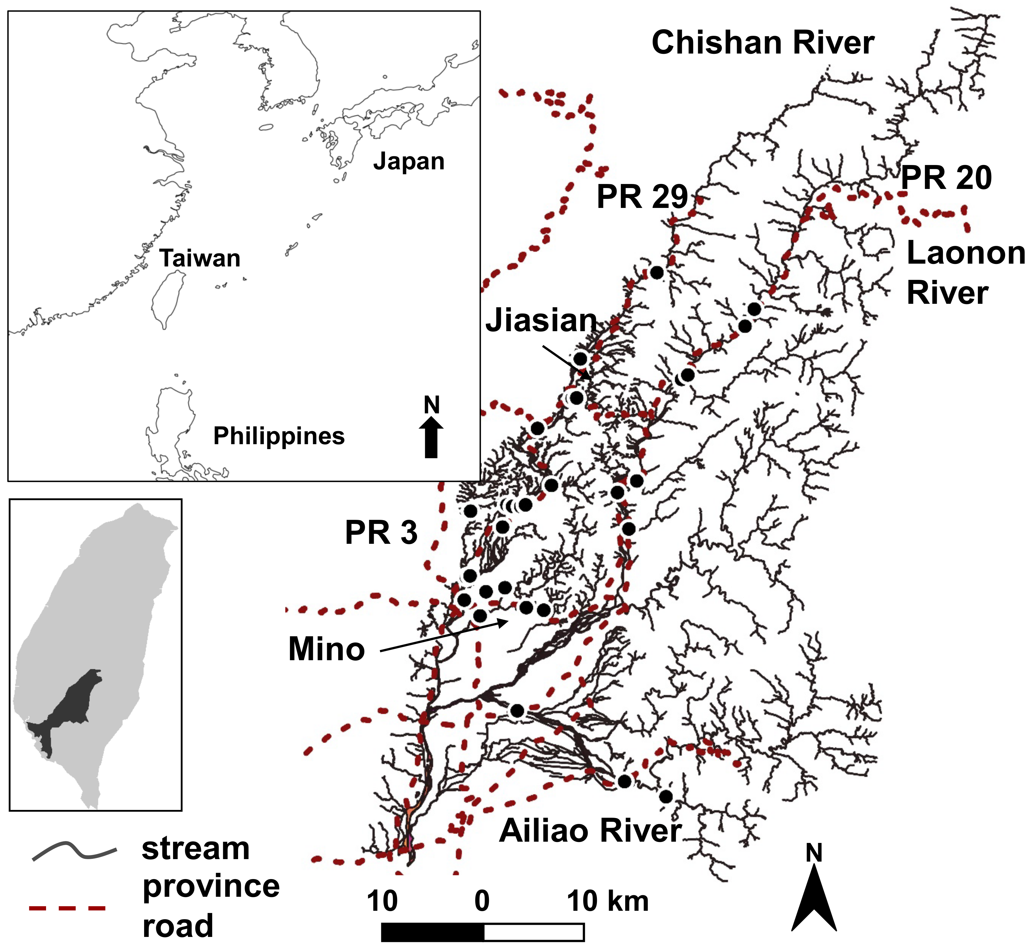
The studied Kaoping River, one of the major rivers in Taiwan, is located between 22.4765° and 23.4894° north in tropical Southern Taiwan. The annual average air temperature is 24.9 °C, with the lowest temperature in January and the highest in July [31]. The mean annual precipitation is 3046 mm, with 90% occurring between April and October during the typhoon and rainy season (The Seventh River Management Office, 2009). The Kaoping River consists of two main tributaries: the Chishan River and Laonon River (Figure 1). The land use of the Chishan River watershed has about 53.9% forest, 41% agriculture, and 5.1% built land [32]. The Laonon River consists of the Upper Laonon River and Ailiao River. The Upper Laonon River watershed comprises 85% forest, 9.7% agriculture, and 5% built land; the Ailiao River watershed consists of 71% forest, 23.8% agriculture, and 4.9% built land [32]. The average slope of the mainstem river is 0.7%.
The Jiasian weather station (in the Chishan River watershed) of the Taiwan Central Weather Bureau recorded the monthly mean temperature and accumulated rainfall in 2009 and 2010 (Appendix A). A record-breaking typhoon, Morakot, hit Taiwan from 6 to 10 August 2009 [33]. Morakot produced a record high accumulated rainfall in a single day (800 mm) and over two days (about 2000 mm) [34], and created massive landslides in the Kaoping River watershed [35]. Scarce rainfall was present before the pre-typhoon sampling in the dry season. Before the post-typhoon sampling in 2010, five typhoons hit Taiwan between August 30 and October 23 (Taiwan Central Weather Bureau). Three were mild, and two were at moderate levels. Only one, Fanapi, passed through the study catchment from September 19 to 20. Fanapi had the highest center windspeed of 45 m/s, an accumulated rainfall of 499.5 mm within 32 h, and a total rainfall of 1079.5 mm in three days at the Kaohsiung weather station (Taiwan Central Weather Bureau). The damage caused by Fanapi included 2 deaths, 111 injuries, 16,000 people evacuated, and TWD 3.4 billion in agriculture [36].
2.2. Physical Habitat and Water Quality Survey
We first selected sampling sites based on Google Maps and then finalized them by field reconnaissance (Figure 1). Site selection criteria in the field included river accessibility, wadeability, no engineering construction immediately upstream or downstream, and presence of both slow and fast channel units. We selected 30 sampling sites that met such criteria, 20 sites from Chishan River and 10 sites from Laonon River.
Physical habitats were surveyed primarily based on the methods described by Kaufmann and Robison [37] and Kaufmann et al. [38] during March and December 2010, before and after the typhoon seasons. At each site, we delineated a 100 m reach consisting of 11 transects 10 m apart. Physical habitats were measured at five evenly spaced points on each transect, including substrate size, water depth, current velocity, canopy cover, and fish cover. Substrata sizes and water depths were measured at each point of transect with a meter stick [39]. Current velocities were measured using a flow meter (FP101 flow probe, Global Water™, Yellow Springs, OH, USA). Fish cover and habitat complexity were assessed semi-quantitatively as five categories (0%, <10%, 10–40%, 40–75%, and >75%) [37], which included % of filamentous algae cover, woody debris, aquatic macrophytes, and boulder and rock ledges.
Stream width was measured using a measuring tape when the stream width was less than 10 m, and measured using a laser rangefinder for widths greater than 10 m (800S, Nikon™, Taipei, Taiwan). We measured the bankfull height using a meterstick and the bankfull width and floodplain width at two times bankfull height (flood-prone width) using a laser rangefinder. We then calculated the entrenchment ratio as flood-prone width/bankfull width [40].
At each site, water discharge was calculated based on water depth measurements and current velocities at 60% of the water depth and at every 0.5 m distance point on a wadeable transect with relatively smooth substrata. Stream slope was measured as the height difference between the upstream and downstream ends of a site and was measured using a leveler and meter rods. Channel units were classified as cascade, rapid, riffle, glide, and pool, and then they were converted into the area percentage of each type according to the definition of Kaufmann and Robinson [37]. We also measured elevation using a handheld GPS (GPSmap, 60CSx, Garmin™, Taipei, Taiwan) and evaluated stream order and sinuosity of a site using 1/50,000 maps. We calculated sinuosity by dividing a 5 km stream length (encompassing the site) by its straight distance.
At each site, we also measured water temperature, pH, conductivity, and salinity using a water quality meter (model 63, YSI™, Yellow Springs, OH, USA), dissolved oxygen using a DO probe (Oxi 340i, YSI™, Yellow Springs, OH, USA), and turbidity using a turbidity meter (TURB 355T, WTW™, Weilheim, Germany). A 500 mL water sample was taken at each site, stored on ice in a dark cooler, and shipped to the lab for analysis.
In the lab, NH4+-N and NO3−-N were analyzed using a water quality instrument (NOVA 60, Merck™, Kenilworth, NJ, USA), whereas NO2−-N and PO4−3-P were analyzed using a spectrophotometer (Cintra 20l, GBC™, Braeside, Australia). NO2−-N was analyzed at a 543 nm wavelength and PO4−3-P at a 700 nm wavelength. Turbidity was measured with a turbidity meter. Suspended solids were measured using the NIEA drying method (NIEA W210.58A, Taoyuan, Taiwan).
The riparian conditions included canopy cover, riparian vegetation structure, and human influence in the riparian area. Canopy cover was measured using a densiometer (Forestry Suppliers™, Jackson, MS, USA). Midstream canopy densities were measured in four directions (upstream, downstream, left, and right), whereas bank canopy densities were measured facing banks at wet margins (left and right).
Riparian vegetation was conceptually divided into three layers: a canopy layer (>5 m high), an understory (0.5 to 5 m high), and a ground cover layer (<0.5 m high), whereas large and small diameter trees were separated in the canopy layer as herbaceous and woody vegetation in the understory layer [37]. The maximum cover in each layer was 100%; thus, the sum of the areal covers for the combined three layers can add up to 300%. The five choices for areal cover of each vegetation layer were “0” (absent: zero cover), “1” (sparse: <10%), “2” (moderate: 10 to 40%), “3” (heavy: 40 to 75%), and “4” (very heavy: >75%) [38].
The human disturbance was visually estimated at the 10 m riparian zones on both sides of the river [38]. Types of human disturbance included channel revetment, buildings, pavement, roads, pipes, row-crop agriculture, and total agriculture.
2.3. Fish Survey
Fish were sampled in March and December 2010 during the two dry seasons before and after the typhoon season. We sampled only dry seasons because the high water level in the wet season prevented site access. A backpack electrofishing unit was used to survey the 100 m stream reach. Fish sampling went downstream to upstream in a zigzag manner and lasted 1–1.5 h at each site, depending on the size of the streams. Captured fish were identified and their length and weight were recorded, then they were released into the streams. Unidentifiable fish were preserved with 10% formalin to be identified according to Shen and Wu [41] in the lab. Fish sampling was conducted with permits from the local government, the Forestry Bureau, and the Fisheries Agency.
2.4. Data Analyses
To evaluate whether the overall fish communities and habitat measures differed before and after the typhoon flood season, we first examined if the sampling sites were similar in ordination spaces using symmetric Procrustes analysis to rotate and superimpose the ordination of one season to another season [43]. The Procrustes test was calculated with the solution of the two first principal components and assessed by a test with 999 permutations. We then conducted paired t-tests on physical habitat, water quality, and riparian condition variables for sites between the two sampling seasons. We also compared fish species occurrence, individual species abundance, and 14 additional fish community metrics between the two sampling seasons using paired t-tests. We calculated the beta diversity as Whittaker’s beta [44], γ/α, where α is the average number of species per site, and γ is the total number of species collected. We lastly evaluated if the associations between fish communities and habitat variables differed between the two seasons by correlating habitat variables with the four fish metrics that were different between the two seasons (identified in the early step) using Spearman rank correlations.
To evaluate how habitat factors affected fish communities before and after the typhoon season, we conducted canonical correspondence analysis (CCA) on three datasets (pre- and post-typhoon season, and the two seasons combined) using three fish measures (presence–absence, abundance, and fish metrics) as dependent variables and habitat variables as independent variables. Abundance data were square-root transformed. We used CCA since the preliminary detrended correspondence analysis (DCA) showed that the gradient lengths of the first axis for all datasets were higher than the four standard deviations [45]. We used the forward selection to select habitat variables with the inclusion criteria of p < 0.05 [46]. The biplot of the 1st and 2nd axes were examined. These analyses used the vegan package [47] of the R software (Version 3.3.1, R Foundation for Statistical Computing, Vienna, Austria).
To assess the relative contributions of the three habitat types (physical, water quality, and riparian conditions) to the variation of the three fish measures before and after the typhoon season, we first used forward selections to identify the first five variables of each habitat type for each of the fish measures to be included in CCA in each season [46]. For fair comparisons, we tried to select similar numbers of variables. Rare species at a <3 occurrence or accumulated individuals <6 were removed from these analyses because canonical analyses are sensitive to rare species [48]. We then used variation partition to quantify the variation contributed by each habitat type and interactions among habitat types in explaining the variation of fish measures [49].
3. Results
3.1. Differences in Physical Habitat, Water Quality, Riparian Conditions, and Fish Measures between the Pre-Typhoon and Post-Typhoon Seasons
The sampling sites had considerable variations in elevation (38–553 m), stream order (1–5), width (1.3–47.6 m), dissolved oxygen (1.3–8.3 mg/L), and riparian agricultural land use (0–44%) (Table 2). Among the 44 physical habitats, water quality, and riparian variables, ten significantly differed between the pre- and post-typhoon seasons (Table 2). Among them, the width-to-depth ratio, percent of rapids, phosphate, water temperature, turbidity, suspended solids, and bank canopy density were significantly higher in the pre-typhoon than in the post-typhoon season. In contrast, the percent of run, total inorganic nitrogen, and pH were significantly higher in the post-typhoon than in the pre-typhoon season.
Our study collected 5 orders, 11 families, and 32 species of fish. Twenty-four were native, eight were invasive, and four were migratory species (Table 3). In the pre-typhoon season, the dominant species were the Southern Taiwan goby (Rhinogobius nantaiensis) (21.6%), Formosan river loach (Hemimyzon formosanus) (21.5%), and freshwater minnow (Opsariichthys pachycephalus) (13.9%). A total of 28 species were caught, with an average of 4.9 species per site and Whittaker’s beta diversity of 5.68. In the post-typhoon season, the dominant species were the same but had lesser dominancy, with 14.3% being Formosan river loach, 14.3% freshwater minnow, and 11.0% Southern Taiwan goby. A total of 26 species were caught, with an average of 3.8 species per site and Whittaker’s beta diversity of 6.84.
Among the 32 fish species collected, 6 species (2 invasive, 2 catadromous, and 2 native species) were collected only during the pre-typhoon season. Three native and one invasive species were collected only during the post-typhoon season (Table 3). The species collected from only one season were generally in small abundance (average < 0.1 fish/site), except for the Taiwan shovel-jaw carp (Onychostoma barbatulum) and red-spotted goby (Rhinogobius rubromaculatus), which had averages of 0.17 and 0.43 per site, respectively.
Among the 16 fish community metrics, 4 were significantly different between the two seasons (Table 1). Species richness in the pre-typhoon season was higher than that in the post-typhoon season (p = 0.03), and the total number of fish caught per site was 35.5 individuals higher in the pre-typhoon than in the post-typhoon season (p = 0.001). Percentages of benthic fish were 13.3% higher in the pre-typhoon than in the post-typhoon season (p = 0.016), whereas portions of sub-benthic fish were 9.7% less in the pre-typhoon season than in the post-typhoon season (p = 0.021).
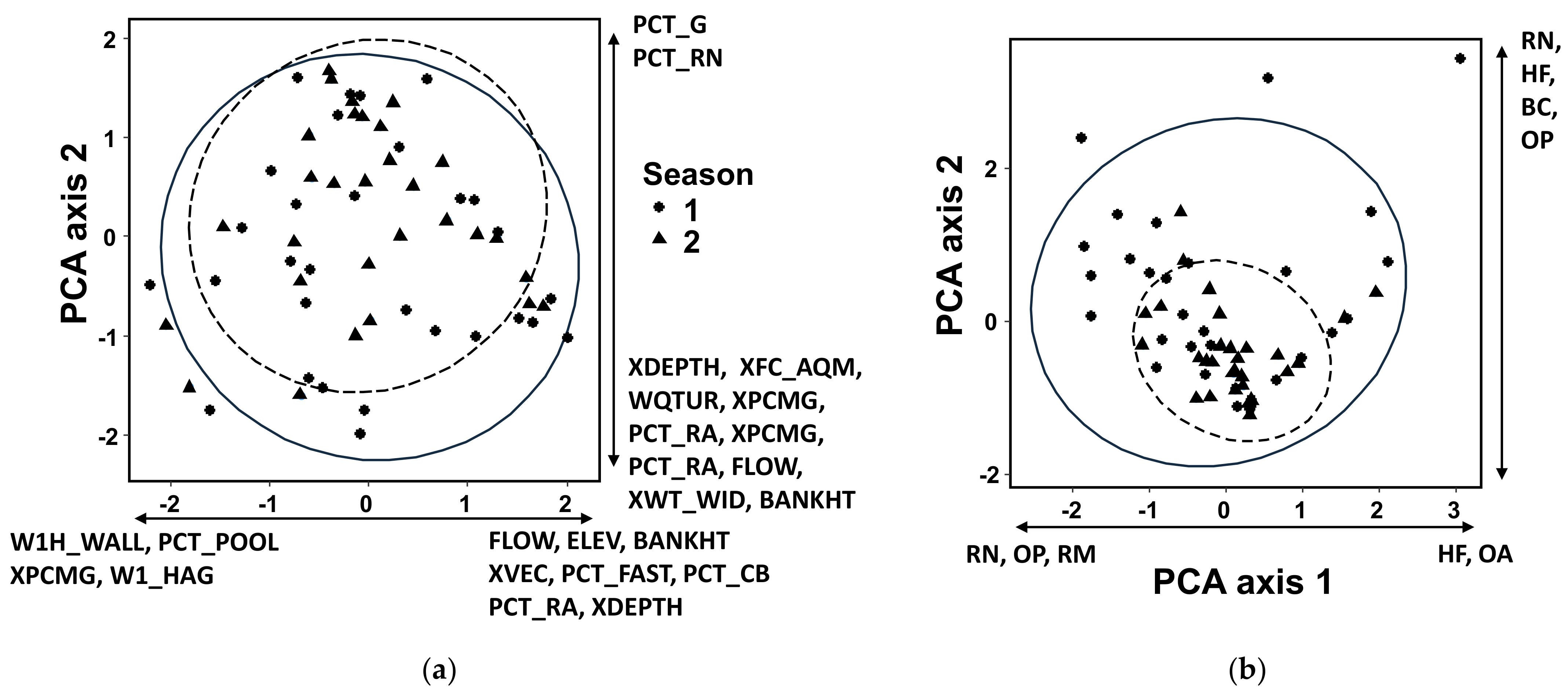
Procrustes tests showed that habitat variables and fish community compositions between the two seasons were significantly different in the ordination space (habitat: sum of square = 0.39, p = 0.001; fish: sum of square = 0.72, p = 0.002) (Figure 2). In the biplot, the difference between the fish compositions of the two seasons was larger than that of habitat measures.
3.2. Associations among Environmental Factors and Fish Community Measures
Thirty-six of the forty-four physical habitat, water quality, and riparian variables were significantly correlated with at least one of the fish community measures between the two seasons (Table 4). When all correlations of the pre-typhoon and post-typhoon seasons and the two seasons combined were considered together, elevation and riparian vegetation were consistently correlated with species richness; water depth and velocity, dissolved oxygen, and water temperature were strongly correlated with benthic or sub-benthic fishes; and physical habitat variables that correlated with fish abundance varied between the two seasons and the two seasons combined (Table 4).
3.3. Key Environmental Variables Associated with Fish Communities
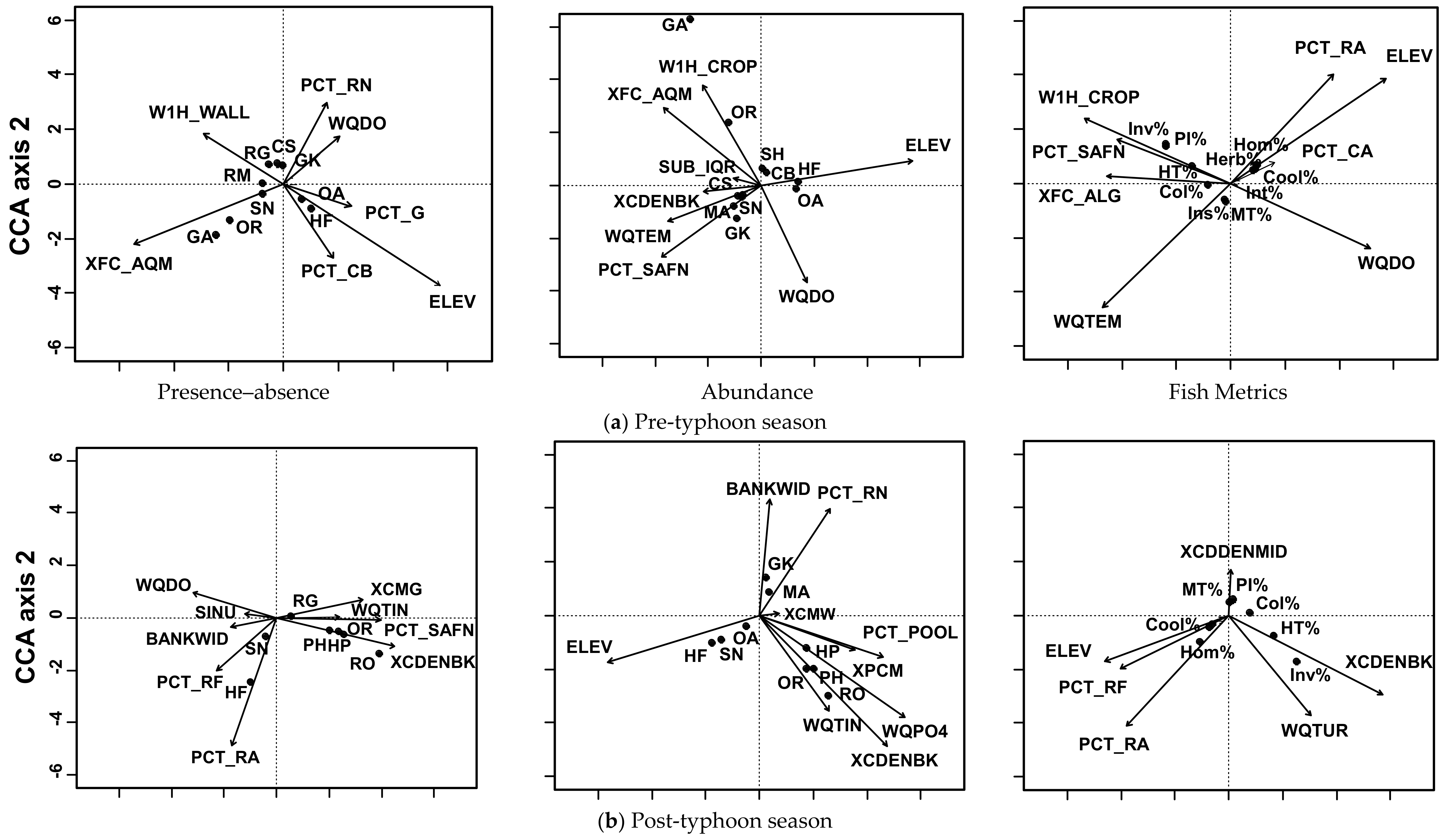
For the pre-typhoon season, the seven selected habitat variables explained 53.5% of the fish presence; eight variables explained 71.2% of the abundance and 72.8% of the community metric variations (Figure 3a). The presence of Formosan river loach and deep-body shovelnose minnow (Onychostoma alticorpus) were positively related to elevation and gravel and cobble substrates. Presences of mosquitofish (Gambusia affinis) and tilapia (Oreochromis sp.) were associated with aquatic vegetation cover, whereas the presence of Hainan eight-barbel gudgeon (Gobiobotia intermedia) was related to dissolved oxygen and run habitat. Abundances of Formosan river loach and deep-body shovelnose minnow were also positively related to elevation, whereas Hainan eight-barbel gudgeon was positively associated with water temperature and sand-fine substrate. Abundances of mosquitofish and tilapia were positively related to agricultural land and aquatic vegetation and negatively associated with dissolved oxygen. Percentages of cool-water, homalopterid, intolerant, and herbivore individuals were positively associated with elevation and the percent of rapids and negatively related to water temperature. Percentages of piscivore/insectivore, invasive, highly tolerant, and water column fish were positively related to agricultural land, sand-fine substrate, and benthic algae, but negatively related to dissolved oxygen.
For the post-typhoon season, the ten selected habitat variables explained 61.8% of the fish presence, nine variables explained 60.9% of the abundance, and six variables explained 59.8% of the fish community metrics (Figure 3b). The presence of Formosan river loach was positively related to rapids and riffle habitats. Rosy bitterling (Rhodeus ocellatus) and tilapia were positively related to bank canopy density and sand-fine substrate, and negatively associated with dissolved oxygen. Abundances of Formosan river loach and Southern Taiwan sucker loach were positively related to elevation. Abundances of rosy bitterling, tilapia, and Taiwan bitterling were positively related to bank canopy density, phosphate, and total inorganic nitrogen, whereas Hainan eight-barbel gudgeon was positively related to the bankfull width. Percentages of homalopterid individuals were positively related to rapids, riffle habitat, and elevation. Percentages of invasive and highly tolerant individuals were positively related to bank canopy and turbidity. The percentage of insectivore individuals was positively associated with midchannel canopy density.
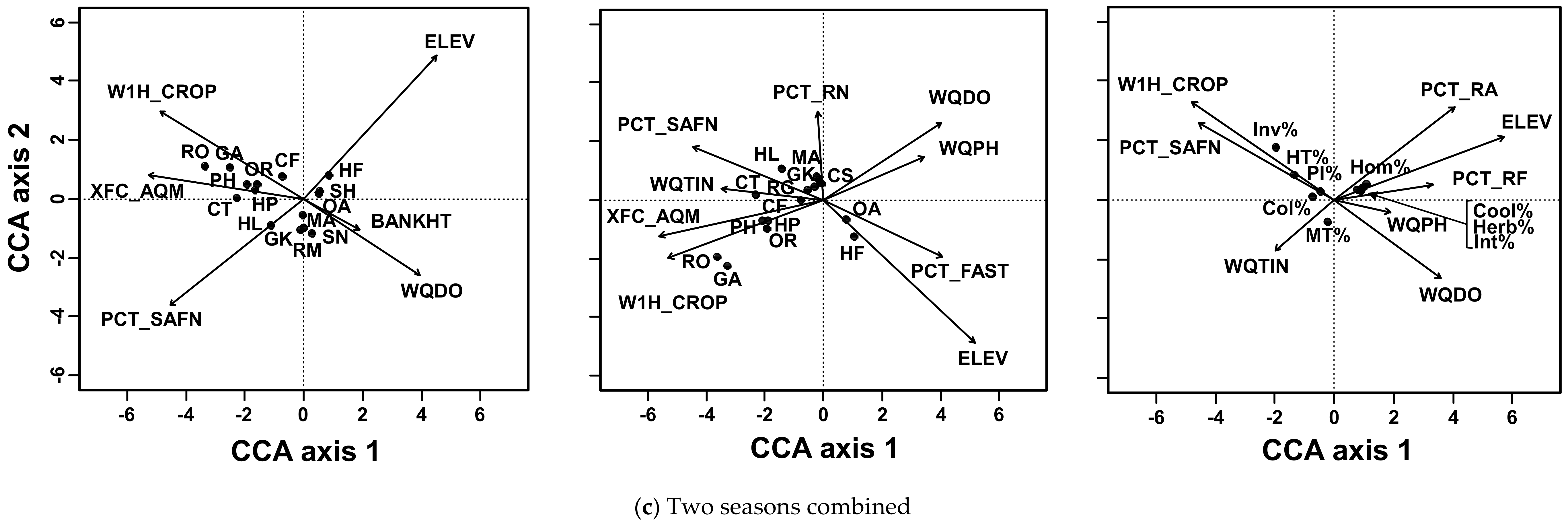
For the two seasons combined, 10 selected habitat variables explained 29.7% of the fish presence, 11 variables explained 44.1% of the fish abundance, and 9 variables explained 55.0% of the fish metrics (Figure 3c). The presence of Formosan river loach was positively related to elevation, and sharpbelly (Hemiculter leucisculus) was positively related to sand-fine substrate. Rosy bitterling and mosquitofish were positively associated with aquatic vegetation and riparian agricultural land. Formosan river loach and deep-body shovelnose minnow abundances were positively related to elevation and a percent of fast-water habitat, whereas sharpbelly and snakehead murrel (Channa striata) were positively related to sand and fine substrata and total inorganic nitrogen. Abundances of rosy bitterling and mosquitofish were positively related to riparian agricultural land and aquatic vegetation, but negatively associated with dissolved oxygen and pH. The percentages of invasive and highly tolerant individuals were positively related to agricultural land and sand-fine substrate, and negatively associated with dissolved oxygen. The percentages of homalopterid, cool-water, herbivore, and intolerant individuals were positively related to elevation, rapids, and riffle, and negatively related to total inorganic nitrogen.
3.4. Partitioning Variation of Fish Communities among Three Habitat Types
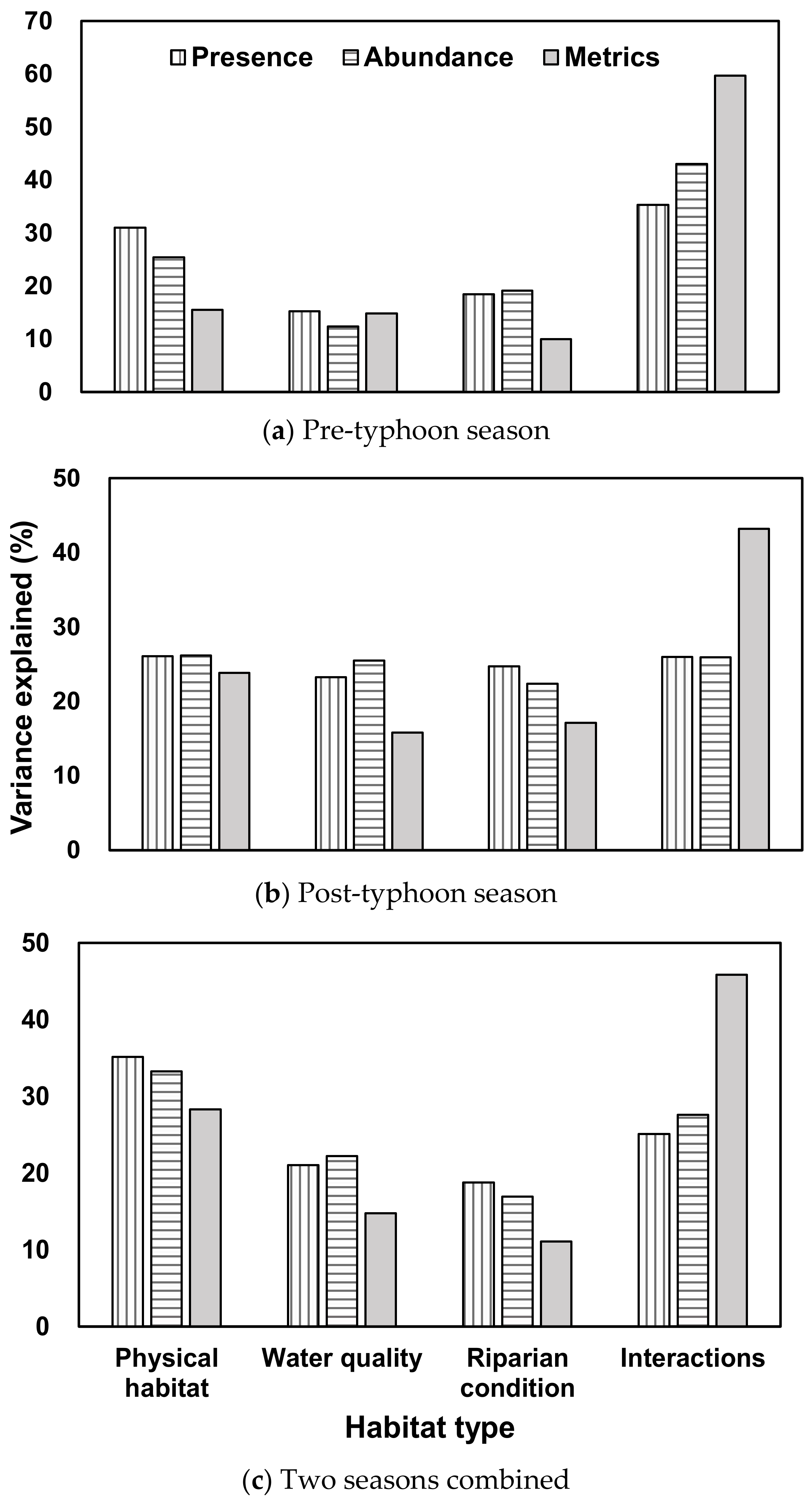
For the pre-typhoon season, 15 selected variables explained a 71.3% variation in fish presence. Among the explained variance, physical habitats explained the most (31%) (the sole contribution without interactions with other habitat types), riparian condition (18%) and water quality (15%) variables explained a similar amount, and the interactions among the three environmental categories explained 36% (Figure 4a). Fifteen selected habitat variables explained an 80.8% variation in fish abundance. Physical habitats (25%), riparian variables (19%), water quality variables (12%), and the interactions among the three habitat types (43%) explained a similar amount of variation. Fifteen selected variables explained a total of 78.5% variation of the fish metrics. Physical habitats (16%), riparian variables (16%), and water quality (15%) explained less variance than the interactions among the three habitat types (25%).
For the post-typhoon season, 15 selected habitat variables explained a 69.4% variation in fish presence. Among the explained variance, physical habitat (26%), riparian conditions (25%), and water quality (23%) explained much less variance than interactions among the three habitat types (26%) (Figure 4b). Fifteen selected variables explained a total of 68.7% variation in fish abundance. Physical habitats (26%), riparian conditions (22%), water quality (25%), and the interactions among the three habitat types (26%) explained a similar amount of variation. Fifteen selected habitat variables explained a 76.1% variation of the fish metrics. Physical habitats explained the most (24%), and riparian conditions (17%) and water quality (16%) explained a similar amount, but they explained much less variance than the interaction among the three habitat types (43%).
For the two seasons combined, 27 selected habitat variables explained a total of 58.4% variation in fish presence. Among the explained variance, physical habitat (35%), water quality (21%), and riparian conditions (19%) explained much less than interactions among the three habitat types (25%) (Figure 4c). Twenty-eight selected variables explained a total of 62.9% variation in fish abundance. Physical habitats (33%), water quality (22%), and riparian conditions (17%) explained less than the interactions among the three habitat types (28%). Twenty-eight selected variables explained a 72.8% variation in fish community measures. Physical habitats explained the most (28%), water quality (15%), and riparian conditions (11%) explained a lower amount, and the interactions among the three habitat types (46%) explained the highest amount of variation of fish metrics.
4. Discussion
4.1. Typhoon Influences on Fish and Habitat
The overall differences measured in fish composition and habitat between the sites sampled in the pre- and post-typhoon seasons support the hypothesis that the relative strengths of biotic and abiotic mechanisms of community assembly can be regulated by the course of the intra-annual hydrologic variation. Although it has been well documented that catastrophic floods can seriously damage instream and riparian habitats and residential fish assemblages in mountain streams [50,51,52], the larger difference in fish compositions than habitat variables between the pre- and post-typhoon seasons implies that such an intra-annual hydrologic variation had a stronger direct impact on fish compared to the indirect influence through impacts on habitat. Although lotic fish communities have evolved with dynamic geomorphological conditions and are relatively resilient to extreme hydrologic events [53,54], severe floods may reduce fish presence, abundance, and influence community compositions [55]. These findings are consistent with our results, implying that fish community compositions have a high fluctuation of abundances due to direct responses to flood disturbance and flood-resulted habitat alteration such as sediment movement, water movement, rearrangement of stream morphology, and riparian vegetation.
The habitat difference between the pre- and post-typhoon seasons is mainly related to channel morphology (e.g., width/depth ratio, % riffle or % run), water quality (e.g., concentrations of nutrients, turbidity, and suspended solids), and bank vegetation density. Such differences might be partly the product of the flood influences of the previous year. Higher turbidity, suspended solids, and phosphate in the pre-typhoon season might be related to the flood disturbance of the Morakot typhoon of the previous year, which produced high rainfall and landslides and increased sediments in the water over an extended period [56]. The typhoon-induced disturbance in the study year changed the physical habitat from wide-rapids to run-dominated habitats. A higher pH in the post-typhoon season might be related to higher benthic algae, which could have resulted from an open canopy and higher inorganic nitrogen conditions.
There is a clear difference in fish communities between pre-typhoon and post-typhoon seasons, despite several studies showing the high resilience of tropical fish communities [25,26,57]. Typhoon Fanapi hit Taiwan late in the typhoon season, three months before fish sampling. The number of fish species per site, total number of fish caught per site, and percent of benthic fish significantly declined after the flood season due to an accumulated rainfall of 2892 mm in the typhoon season (Appendix A). The reduction in the percent of benthic fish in the post-typhoon season may indicate that they were vulnerable during the flood season. These fish often stayed on or hid under substrata which would be moved during high floods and likely caused high mortality. Despite an overall decrease in the number of fish caught in the post-typhoon season, the percent of sub-benthic fish increased, which may indicate their higher escaping capability and a reduction in competition from benthic fish during the recovery process. Our results improved our knowledge about sub-benthic fish being vulnerable during the flood season and capable of recovering afterward.
4.2. Fish–Habitat Relationships between Pre-Typhoon and Post-Typhoon Seasons
Measured habitat variables explained high proportions of fish community variation, with a higher variation explained for pre- than post-typhoon seasons. The amount of total variance explained in this study was over 50% with less or equal to 10 habitat variables. From vegetation studies, the total variance explained was generally between 20 and 50%, and a larger variance would be explained when beta diversity was small [58]. In this study, Whittaker’s beta was 5.7 and 6.8 for the two seasons, despite only 4.4 fish species per site. Compared with the Northern Lake and Forests ecoregion study in the USA [1], the fish variance explained was from 40 to 51%, with 12 species per site, and Whittaker’s beta was 5.1. The current study had a higher amount of variance explained under lower species richness. Beta diversity cannot explain the amount of variance explained in this case. Other factors, such as strong environmental gradients and non-nested species distribution, may have contributed to the high variance explained. The reasons for the amount of fish variance explained deserve further study. In addition, a longer recovery time for fish may increase the variance explained by habitat variables. The fish variance explained by habitat variables was higher in the pre-typhoon than the post-typhoon season, probably because fish in the pre-typhoon season had a longer recovery time from the previous flood disturbance.
Key environmental variables associated with fish communities differed between the two sampling seasons. In the pre-typhoon season, elevation and agriculture were the two major factors affecting fish communities, whereas gradients related to habitat, bank vegetation cover, and water quality were the key factors influencing the post-typhoon season. In addition, the pre-typhoon season generally had more community variance explained than the post-typhoon season, which probably showed a recovery from the disturbance of the typhoon season. Furthermore, when data from the two seasons were combined, habitat variables had the lowest fish variance explained. These results showed that core environmental gradients, such as elevation–substrata and crop–DO gradients, structured fish communities regardless of the season.
Our results show that fish assemblages were highly related to the physical habitat in dry seasons, which contradicts our original hypotheses that fish may not respond to physical habitat. The possible explanation is that fish may adapt as habitat-generalists to survive during the physical flood disturbance, but are physical habitat-specialists in the dry season. From observations and experiments, fish can escape to tributaries during a flood event [59], which may require behavioral plasticity to adapt to habitats of tributaries temporarily. The length of the dry season, commonly from October to March, is as long as the wet season. Fish may need to adapt to resource limitations and competition in the dry season, consequently conforming to certain physical habitat factors as a way of partitioning resources [11,60]. In addition, these fish still need to partition their physical habitat along longitudinal gradients to reduce competition and recover their populations [61,62].
The fish variation explained by physical habitats overwrites that of water quality and riparian conditions. In the study region, the impairment of water quality was influenced by a mild level of agriculture and residential land uses. The degradation of water quality was not serious enough to strongly affect fish communities. Riparian zones also had a minor role in affecting fish communities and physical habitats. These streams have a high magnitude and frequency of hydrological disturbance [15], with the primary force shaping stream geomorphology and riparian habitats [63]. This hydrological disturbance regime can erode riparian areas, consequently reducing the connectivity between riparian and stream channels [64]. These streams had low canopy cover, which may indicate erosion. Thus, the shared variance between riparian and physical habitat variables in explaining fish communities were small.
The environmental filtering model may explain the assembly of fish communities in these tropical streams. As revealed by CCA results, several dominant fish species had consistent relationships with habitat factors. For example, the Formosan river loach was positively related to elevation and associated factors, whereas tilapia was positively related to higher sand-fine substrata and canopy cover in agriculture areas. Fish communities were structured by habitat factors in the dry seasons, which is partially contrary to the statement that communities may be structured by stochastic factors in the dry season [24]. Zbinden and Mathews [65] also suggested that fish assemblages are structured by environmental filtering in southeastern Oklahoma.
Our results have substantial implications for stream bioassessment and management. Based on the high variances of fish communities explained by habitat factors, bioassessments are feasible in these typhoon-affected tropical streams. Despite fish community metrics being related to habitat factors in CCA results, two natural elements need to be considered in the bioassessment program. First, natural variations, such as elevation-related factors, need to be separated from human disturbance by establishing stream typology [66]. Second, the rainy season may not be appropriate for assessment because the sampling is often under high flow and is unsafe for crews. Physical habitats may be the priority for stream management because they may maintain fish diversity. Tributary habitats may serve as refuge during floods, and hence, need to be protected from disconnections to mainstreams and habitat modifications. In addition, water quality and the riparian conditions that explained certain levels of fish variance might also be necessary when they are moderately or severely degraded. Furthermore, invasive species are present in human-modified streams. These invasive species are widespread in Taiwan and dominant in specific streams [12,67]. Restoring physical habitats and minimizing flood disturbance may be an option for abating invasive species and maintaining native fish communities [57]. Whether restoration measures effectively control or decimate invasive species in this region requires further study.
5. Conclusions
Habitat factors and fish community measures in the typhoon-affected mountain streams differed between pre-typhoon and post-typhoon seasons. Overall, community compositions had larger deviations than habitat variables between the two seasons. The benthic fish guild was more vulnerable to flood impacts than other guilds. Habitat factors, especially physical habitats, were strongly related to fish community measures, indicating the dominance of environmental filtering. Habitat factors explained more variance for fish metrics than for other fish measures. The fish–habitat relationships slightly differed between pre-typhoon and post-typhoon seasons. Our findings of seasonal fish–habitat relationships and the influences of landscape–climate conditions on such relationships provide the basis for developing conservation and bioassessment programs for typhoon-prone tropical mountain streams.
Author Contributions
Y.-K.W. and R.-L.K. contributed to the methodology, implementation, and data curation. Y.-K.W. also contributed to the conceptualization, resources, and supervision. Y.-K.W. and L.W. contributed to the formal analysis and writing. All authors have read and agreed to the published version of the manuscript.
Funding
This research received no external funding.
Data Availability Statement
Not applicable.
Acknowledgments
We would like to thank I-Jie Tsai, Ron-Kai Su, Yu-Yu Chen, Ya-Fen Chang, Hua-Yu Wang, Jun-Fan Chien, Shin-Fu Chen, Shi-Tin Yan, Yin-Che Chiu, and Wen-Yan Fan for their help with field and lab work and Fan-Rou Liu for the discussion on data analysis. We would like to thank Min-Tai Chou for discussions on fish taxonomy and ecology. This study was partly supported by the National University of Tainan.
Conflicts of Interest
The authors declare no conflict of interest.
Appendix A
Figure A1.
The monthly mean temperature and accumulated rainfall of the Jiasian weather station (in the middle reach of the Kaoping River) in (a) 2009 and (b) 2010. Data source: Taiwan Central Weather Bureau.
Figure A1.
The monthly mean temperature and accumulated rainfall of the Jiasian weather station (in the middle reach of the Kaoping River) in (a) 2009 and (b) 2010. Data source: Taiwan Central Weather Bureau.

References
- Wang, L.; Lyons, J.; Rasmussen, P.; Kanehl, P.; Seelbach, P.; Simon, T.; Wiley, M.; Baker, E.; Niemela, S.; Stewart, M. Influences of landscape-and reach-scale habitat on stream fish communities in the Northern Lakes and Forest ecoregion. Can. J. Fish. Aquat. Sci. 2003, 60, 491–505. [Google Scholar] [CrossRef]
- Sawyer, J.A.; Stewart, P.M.; Mullen, M.M.; Simon, T.P.; Bennett, H.H. Influence of habitat, water quality, land use on macroinvertebrate and fish assemblages of a southeastern coastal plain watershed, USA. Aquat. Ecosyst. Health 2004, 7, 85–99. [Google Scholar] [CrossRef]
- Vondracek, B.; Blann, K.L.; Cox, C.B.; Nerbonne, J.F.; Mumford, K.G.; Nerbonne, B.A.; Sovell, L.A.; Zimmerman, J.K. Land use, spatial scale, and stream systems: Lessons from an agricultural region. Environ. Manag. 2005, 36, 775–791. [Google Scholar] [CrossRef] [PubMed]
- Wang, L.; Infante, D.; Esselman, P.; Cooper, A.; Wu, D.; Taylor, W.; Beard, D.; Whelan, G.; Ostroff, A. A hierarchical spatial framework and database for the national river fish habitat condition assessment. Fisheries 2011, 36, 436–449. [Google Scholar] [CrossRef] [Green Version]
- López-Delgado, E.O.; Winemiller, K.O.; Villa-Navarro, F.A. Local environmental factors influence beta-diversity patterns of tropical fish assemblages more than spatial factors. Ecology 2019, 101, e02940. [Google Scholar] [CrossRef]
- Tsang, Y.; Infante, D.M.; Wang, L.; Krueger, D.; Wieferich, D. Conserving stream fishes with changing climate: Assessing fish responses to changes in habitat over a large region. Sci. Total Environ. 2021, 755, 142503. [Google Scholar] [CrossRef]
- Karr, J.R. Biological monitoring and environmental assessment: A conceptual framework. Environ. Manag. 1987, 11, 249–256. [Google Scholar] [CrossRef]
- Wang, L.; Brenden, T.; Seelbach, P.; Cooper, A.; Allan, D.; Clark, R., Jr.; Wiley, M. Landscape based identification of human disturbance gradients and references for streams in Michigan. Environ. Monit. Assess. 2008, 141, 1–17. [Google Scholar] [CrossRef]
- Wang, L.; Wehrly, K.; Breck, J.; Kraft, L.S. Landscape based assessment of human disturbance for Michigan lakes. Environ. Manag. 2010, 46, 471–483. [Google Scholar] [CrossRef] [Green Version]
- Dextrase, A.J.; Mandrak, N.E.; Schaefer, J.A. Modelling occupancy of an imperilled stream fish at multiple scales while accounting for imperfect detection: Implications for conservation. Freshw. Biol. 2014, 59, 1799–1815. [Google Scholar] [CrossRef]
- Grossman, G.D.; Freeman, M.C. Microhabitat use in a stream fish assemblage. J. Zool. 1987, 212, 151–176. [Google Scholar] [CrossRef]
- Lin, S.-J.; Tsai, S.-T.; Lin, J.-H.; Jong, K.-J.; Wang, Y.-K. The changes in structure and function of fish assemblages along environmental gradients in an intensive agricultural region of subtropical Taiwan. Pac. Sci. 2014, 68, 213–230. [Google Scholar] [CrossRef]
- Encalada, A.C.; Flecker, A.S.; Poff, N.L.; Suárez, E.; Herrera, G.A.; Ríos-Touma, B.; Jumani, S.; Larson, E.I.; Anderson, E.P. A global perspective on tropical montane rivers. Science 2019, 365, 1124–1129. [Google Scholar] [CrossRef]
- Lewis, W.M., Jr. Physical and chemical features of tropical flowing waters. In Tropical Stream Ecology; Dudgeon, D., Ed.; Academic Press: San Diego, CA, USA, 2008; pp. 1–22. [Google Scholar]
- Teng, W.-H.; Hsu, M.-I.; Wu, C.-H.; Chen, A.-S. Impact of flood disasters on Taiwan in the last quarter century. Nat. Hazards 2006, 37, 191–207. [Google Scholar] [CrossRef] [Green Version]
- Yu, P.S.; Yang, T.C.; Kuo, C.C. Evaluating long-term trends in annual and seasonal precipitation in Taiwan. Water Resour. Manag. 2006, 20, 1007–1023. [Google Scholar] [CrossRef]
- Yang, T.C.; Chen, C.; Kuo, C.M.; Tseng, H.W.; Yu, P.S. Drought risk assessments of water resources systems under climate change: A case study in Southern Taiwan. Hydrol. Earth Syst. Sci. Discuss. 2012, 9, 12395–12433. [Google Scholar] [CrossRef] [Green Version]
- Kao, S.J.; Milliman, J.D. Water and sediment discharge from small mountainous rivers, Taiwan: The roles of lithology, episodic events, and human activities. J. Geol. 2008, 116, 431–448. [Google Scholar] [CrossRef] [Green Version]
- Ostrand, K.G.; Wilde, G.R. Seasonal and spatial variation in a prairie stream-fish assemblage. Ecol. Freshw. Fish 2002, 11, 137–149. [Google Scholar] [CrossRef]
- Stewart-Koster, B.; Kennard, M.J.; Harch, B.D.; Sheldon, F.; Arthington, A.H.; Pusey, B.J. Partitioning the variation in stream fish assemblages within a spatio-temporal hierarchy. Mar. Freshw. Res. 2007, 58, 675–686. [Google Scholar] [CrossRef] [Green Version]
- Espírito-Santo, H.M.V.; Magnusson, W.E.; Zuanon, J.; Mendonça, F.P.; Landeiro, V.L. Seasonal variation in the composition of fish assemblages in small Amazonian forest streams: Evidence for predictable changes. Freshw. Biol. 2009, 54, 536–548. [Google Scholar] [CrossRef]
- Yan, Y.Z.; He, S.; Chu, L.; Xiang, X.Y.; Jia, Y.J.; Tao, J.; Chen, Y.F. Spatial and temporal variation of fish assemblages in a subtropical small stream of the Huangshan Mountain. Curr. Zool. 2010, 56, 670–677. [Google Scholar] [CrossRef]
- Warfe, D.M.; Pettit, N.E.; Davies, P.M.; Pusey, B.J.; Hamilton, S.K.; Kennard, M.J.; Townsend, S.A.; Bayliss, P.; Ward, D.P.; Douglas, M.M.; et al. The ‘wet–dry’ in the wet–dry tropics drives river ecosystem structure and processes in northern Australia. Freshw. Biol. 2011, 56, 2169–2195. [Google Scholar] [CrossRef]
- Fitzgerald, D.B.; Winemiller, K.O.; Sabaj Pérez, M.H.; Sousa, L.M. Seasonal changes in the assembly mechanisms structuring tropical fish communities. Ecology 2017, 98, 21–31. [Google Scholar] [CrossRef] [Green Version]
- Tew, K.S.; Han, C.C.; Chou, W.R.; Fang, L.S. Habitat and fish fauna structure in a subtropical mountain stream in Taiwan before and after a catastrophic typhoon. Environ. Biol. Fish. 2002, 65, 457–462. [Google Scholar] [CrossRef]
- Chuang, L.C.; Shieh, B.S.; Liu, C.C.; Lin, Y.S.; Liang, S.H. Effects of typhoon disturbance on the abundances of two mid-water fish species in a mountain stream of Northern Taiwan. Zool. Stud. 2008, 47, 564–573. Available online: https://zoolstud.sinica.edu.tw/Journals/47.5/564.pdf (accessed on 1 May 2022).
- Adams, S.B.; Warren, M.L.; Haag, W.R. Spatial and temporal patterns in fish assemblages of upper coastal plain streams, Mississippi, USA. Hydrobiologia 2004, 528, 45–61. [Google Scholar] [CrossRef]
- Wang, L.; Seelbach, P.W.; Hughes, R.M. Introduction to landscape influences on stream habitats and biological assemblages. Am. Fish. Soc. Symp. 2006, 48, 1–23. [Google Scholar]
- Resentini, A.; Goren, L.; Castelltort, S.; Garzanti, E. Partitioning sediment flux by provenance and tracing erosion patterns in Taiwan. J. Geophys. Res. Earth Surf. 2017, 122, 1430–1454. [Google Scholar] [CrossRef] [Green Version]
- Liu, J.T.; Kao, S.-J.; Huh, C.-A.; Hung, C.C. Gravity flows associated with flood events and carbon burial: Taiwan as instructional source area. Annu. Rev. Mar. Sci. 2013, 5, 47–68. [Google Scholar] [CrossRef]
- The Seventh River Management Office. The Review of the Master Plan of Improvement of Kaoping River Basin (2009–2014); The Seventh River Management Office of Water Resources Agency of the Ministry of Economic Affairs: Pingtung, Taiwan, 2009. (In Chinese)
- Huang, Y.-J. Richness Conservation of Plant Species by Landscape Ecology in Kao Ping River Basin. Master’s Thesis, National Pingtung University of Science and Technology, Pingtung, Taiwan, 2005. Unpublished (In Chinese). [Google Scholar]
- Wu, L.; Liang, J.; Wu, C.-C. Monsoonal influence on typhoon Morakot (2009). Part I: Observational analysis. J. Atmos. Sci. 2011, 68, 2208–2221. [Google Scholar] [CrossRef]
- Chien, F.C.; Kuo, H.C. On the extreme rainfall of Typhoon Morakot (2009). J. Geophys. Res-Atmos. 2011, 116, D05104. [Google Scholar] [CrossRef] [Green Version]
- Tsou, C.-Y.; Feng, Z.-Y.; Chigira, M. Catastrophic landslide induced by typhoon Morakot, Shiaolin, Taiwan. Geomorphology 2011, 127, 166–178. [Google Scholar] [CrossRef] [Green Version]
- Wikipedia. Typhoon Fanapi. 2010. Available online: https://en.wikipedia.org/wiki/Typhoon_Fanapi (accessed on 9 January 2021).
- Kaufmann, P.; Robinson, E. Physical habitat characterization. In Environmental Monitoring and Assessment Program-Surface Waters: Field Operations and Methods for Measuring the Ecological Condition of Wadeable Streams; Lazorchak, J.M., Klemm, D.J., Peck, D.V., Eds.; U.S. Environmental Protection Agency: Washington, DC, USA, 1998; pp. 77–118. [Google Scholar]
- Kaufmann, P.; Levine, P.; Robinson, E.; Seeliger, C.; Peck, D. Quantifying Physical Habitat in Wadeable Streams; U.S. Environmental Protection Agency: Washington, DC, USA, 1999.
- Wolman, M. A method of sampling coarse river-bed material. Tran. Am. Geophys. Union 1954, 35, 951–956. [Google Scholar] [CrossRef]
- VTDEC. Vermont Stream Geomorphic Assessment Phase 2 Handbook-Rapid Stream Assessment; Vermont Agency of Natural Resources, Water Quality Division: Waterbury, VT, USA, 2009.
- Shen, S.-J.; Wu, G.-Y. Fishes of Taiwa; National Museum of Marine Biology: Chechen, Taiwan, 2009.
- Shannon, C.E.; Weaver, W. The Mathematical Theory of Communication; University of Illinois Press: Urbana, IL, USA, 1949. [Google Scholar]
- Peres-Neto, P.R.; Jackson, D.A. How well do multivariate data sets match? The advantages of a Procrustean superimposition approach over the Mantel test. Oecologia 2001, 129, 169–178. [Google Scholar] [CrossRef]
- Whittaker, R.H. Vegetation of the Siskiyou Mountains, Oregon and California. Ecol. Monogr. 1960, 30, 279–338. [Google Scholar] [CrossRef]
- Ter Braak, C.J.F.; Smilauer, P. Topics in constrained and unconstrained ordination. Plant Ecol. 2015, 216, 683–696. [Google Scholar] [CrossRef] [Green Version]
- Blanchet, F.G.; Legendre, P.; Borcard, D. Forward selection of explanatory variables. Ecology 2008, 89, 2623–2632. [Google Scholar] [CrossRef]
- Oksanen, J.; Guillaume Blanchet, F.; Friendly, M.; Kindt, R.; Legendre, P.; McGlinn, D.; Minchin, P.R.; O’Hara, R.B.; Simpson, G.L.; Solymos, P.; et al. Vegan: Community Ecology Package, R Package Version 2.5–6; 2020. Available online: http://CRAN.R-project.org/package=vegan (accessed on 1 May 2022).
- Poos, M.S.; Jackson, D.A. Addressing the removal of rare species in multivariate bioassessments: The impact of methodological choices. Ecol. Indic. 2012, 18, 82–90. [Google Scholar] [CrossRef]
- Peres-Neto, P.R.; Legendre, P.; Dray, S.; Borcard, D. Variation partitioning of species data matrices: Estimation and comparison of fractions. Ecology 2006, 87, 2614–2625. [Google Scholar] [CrossRef]
- Han, C.C.; Tew, K.S.; Fang, L.S. Spatial and temporal variations of two cyprinids in a subtropical mountain reserve—A result of habitat disturbance. Ecol. Freshw. Fish 2007, 16, 395–403. [Google Scholar] [CrossRef]
- George, S.D.; Baldigo, B.P.; Smith, A.J.; Robinson, G.R. Effects of extreme floods on trout populations and fish communities in a Catskill Mountain river. Freshw. Biol. 2015, 60, 2511–2522. [Google Scholar] [CrossRef]
- Chea, R.; Pool, T.K.; Chevalier, M.; Ngor, P.; So, N.; Winemiller, K.O.; Lek, S.; Grenouillet, G. Impact of seasonal hydrological variation on tropical fish assemblages: Abrupt shift following an extreme flood event. Ecosphere 2020, 11, e03303. [Google Scholar] [CrossRef]
- Nislow, K.H.; Magilligan, F.J.; Folt, C.L.; Kennedy, B.P. Within-basin variation in the short-term effects of a major flood on stream fishes and invertebrates. J. Freshw. Ecol. 2002, 17, 305–318. [Google Scholar] [CrossRef] [Green Version]
- Lytle, D.A.; Poff, N.L.R. Adaptation to natural flow regimes. Trends Ecol. Evol. 2004, 19, 94–100. [Google Scholar] [CrossRef]
- Roghair, C.N.; Dolloff, C.A.; Underwood, M.K. Response of a brook trout population and instream habitat to a catastrophic flood and debris flow. Trans. Am. Fish. Soc. 2002, 131, 718–730. [Google Scholar] [CrossRef]
- Huang, Y.-F.; Montgomery, D.R. Altered regional sediment transport regime after a large typhoon, southern Taiwan. Geology 2013, 41, 1223–1226. [Google Scholar] [CrossRef]
- Smith, W.E.; Kwak, T.J. Tropical insular fish assemblages are resilient to flood disturbance. Ecosphere 2015, 6, 1–16. [Google Scholar] [CrossRef] [Green Version]
- Økland, R.H. On the variation explained by ordination and constrained ordination axes. J. Veg. Sci. 1999, 10, 131–136. [Google Scholar] [CrossRef]
- Koizumi, I.; Kanazawa, Y.; Tanaka, Y. The fishermen were right: Experimental evidence for tributary refuge hypothesis during floods. Zool. Sci. 2013, 30, 375–379. [Google Scholar] [CrossRef] [Green Version]
- Arrington, D.A.; Winemiller, K.O. Habitat affinity, the seasonal flood pulse, and community assembly in the littoral zone of a Neotropical floodplain river. J. N. Am. Benthol. Soc. 2006, 25, 126–141. [Google Scholar] [CrossRef]
- Paine, M.D.; Dodson, J.J.; Power, G. Habitat and food resource partitioning among four species of darters (Percidae: Etheostoma) in a southern Ontario stream. Can. J. Zool. 1982, 60, 1635–1641. [Google Scholar] [CrossRef]
- Herder, F.; Freyhof, J. Resource partitioning in a tropical stream fish assemblage. J. Fish Biol. 2006, 69, 571–589. [Google Scholar] [CrossRef]
- Stoffel, M.; Wyżga, B.; Marston, R.A. Floods in mountain environments: A synthesis. Geomorphology 2016, 272, 1–9. [Google Scholar] [CrossRef]
- Reckendorfer, W.; Funk, A.; Gschöpf, C.; Hein, T.; Schiemer, F. Aquatic ecosystem functions of an isolated floodplain and their implications for flood retention and management. J. Appl. Ecol. 2013, 50, 119–128. [Google Scholar] [CrossRef]
- Zbinden, Z.D.; Matthews, W.J. Beta diversity of stream fish assemblages: Partitioning variation between spatial and environmental factors. Freshw. Biol. 2017, 62, 1460–1471. [Google Scholar] [CrossRef]
- Aroviita, J.; Mykrä, H.; Muotka, T.; Hämäläinen, H. Influence of geographical extent on typology- and model-based assessments of taxonomic completeness of river macroinvertebrates. Freshw. Biol. 2009, 54, 1774–1787. [Google Scholar] [CrossRef]
- Chen, R.-T.; Ho, P.-H.; Lee, H.-H. Distribution of exotic freshwater fishes and shrimps in Taiwan. Endem. Species Res. 2003, 5, 33–46. (In Chinese) [Google Scholar]
Figure 1.
Locations of sampling sites in the Kaoping Creek catchment, Taiwan. PR is the abbreviation for province road; for example, PR 3 is province road 3. Mino and Jiasian are townships in the watershed.
Figure 1.
Locations of sampling sites in the Kaoping Creek catchment, Taiwan. PR is the abbreviation for province road; for example, PR 3 is province road 3. Mino and Jiasian are townships in the watershed.

Figure 2.
Biplots of principal component analyses of (a) habitat variables and (b) fish compositions of two seasons. Solid ellipses are for the pre-typhoon season, and dashed ellipses are for the post-typhoon season. Species and habitat variables presented have higher influences (absolute loading values) in their respective directions. According to the results of Procrustes tests, habitat variables and fish communities between the two seasons were significantly different in the ordination space (habitat: sum of square = 0.39, p = 0.001; fish: sum of square = 0.72, p = 0.002). Descriptions of abbreviations of habitat variables are in Table 2, whereas explanations of abbreviations of fish metrics are in Table 1.

Figure 3.
CCA biplots of three fish measures of three seasonal data. (a) The pre-typhoon season, (b) the post-typhoon season, and (c) the two seasons combined represented as CCA biplots with corresponding presence–absence, abundance, and community characteristics data. Descriptions of abbreviations of habitat variables are in Table 2, and explanations of abbreviations of fish are in Table 1 and Table 3.


Figure 4.
The percent of fish community variance was explained by physical habitats, water quality, riparian conditions, and interactions for three fish measures in (a) the pre-typhoon season, (b) the post-typhoon season, and (c) the two seasons combined.
Figure 4.
The percent of fish community variance was explained by physical habitats, water quality, riparian conditions, and interactions for three fish measures in (a) the pre-typhoon season, (b) the post-typhoon season, and (c) the two seasons combined.


Table 1.
The range, mean, and standard deviations of fish community metrics. ** = significant at p < 0.01 and * = significant at p < 0.05 by paired t-tests between two seasons (also indicated in bold).
Table 1.
The range, mean, and standard deviations of fish community metrics. ** = significant at p < 0.01 and * = significant at p < 0.05 by paired t-tests between two seasons (also indicated in bold).
| Fish Metrics | Abbreviations | Pre-Typhoon Season | Post-Typhoon Season | ||
|---|---|---|---|---|---|
| Range | Mean ± SD | Range | Mean ± SD | ||
| Number of fish species * | NFS | 1–11 | 4.9 ± 2.6 | 1–8 | 3.8 ± 2.0 |
| Fish abundance (individuals/100 m) ** | ABN | 1–212 | 57.7 ± 56.1 | 1–67 | 22.2 ± 20.4 |
| Shannon–Wiener diversity | SW | 0–1.9 | 1.0 ± 0.5 | 0–1.8 | 0.9 ± 0.5 |
| Invasive individuals% | Inv% | 0–100 | 8.1 ± 24.6 | 0–100 | 5.3 ± 19.8 |
| Benthic individuals% * | Ben% | 0–100 | 66.1 ± 30.9 | 0–100 | 52.8 ± 35.0 |
| Water column individuals% | Wcol% | 0–100 | 26.3 ± 29.7 | 0–100 | 30.0 ± 31.8 |
| Sub-benthic individuals% * | Sben% | 0–40 | 7.6 ± 9.9 | 0–80 | 17.3 ± 21.0 |
| Highly tolerant individuals% | HT% | 0–100 | 17.0 ± 29.5 | 0–100 | 15.4 ± 32.2 |
| Intolerant individuals% | Int% | 0–100 | 31.1 ± 40.4 | 0–100 | 27.6 ± 36.2 |
| Medium tolerant individuals% | MT% | 0–100 | 51.9 ± 38.6 | 0–100 | 57.1 ± 39.9 |
| Herbivore individuals% | Herb% | 0–32.9 | 3.6 ± 7.6 | 0–26.9 | 2.7 ± 6.6 |
| Insectivore individuals% | Ins% | 0–100 | 48.8 ± 37.1 | 0–100 | 41.9 ± 32.8 |
| Omnivore individuals% | Omn% | 0–100 | 42.5 ± 34.2 | 0–100 | 45.9 ± 36.8 |
| Piscvore/insectivore individuals% | PI% | 0–100 | 5.1 ± 18.3 | 0–80 | 9.5 ± 17.8 |
| Homalopterid individuals% | Hom% | 0–100 | 22.8 ± 35.8 | 0–100 | 19.7 ± 36.6 |
| Cool-water individuals% | Cool% | 0–100 | 25.9 ± 40.3 | 0–100 | 25.6 ± 36.9 |
Table 2.
The range, mean, and standard deviations of instream physicochemical and riparian land-use measures. ** indicates a significant difference at p < 0.01, and * indicates a significance at p < 0.05 by the paired t-test between pre- and post-typhoon seasons (also shown in bold).
Table 2.
The range, mean, and standard deviations of instream physicochemical and riparian land-use measures. ** indicates a significant difference at p < 0.01, and * indicates a significance at p < 0.05 by the paired t-test between pre- and post-typhoon seasons (also shown in bold).
| Categories and Variables | Codes | Pre-Typhoon Season | Post-Typhoon Season | ||
|---|---|---|---|---|---|
| Range | Mean ± 1SD | Range | Mean ± 1SD | ||
| Physical habitat | |||||
| Elevation (m) | ELEV | 38–553 | 190.9 ± 154.4 | 38–553 | 190.9 ± 154.4 |
| Stream order | STRLEV | 1–5 | 3.5 ± 1.2 | 1–5 | 3.5 ± 1.2 |
| Sinuosity | SINU | 1.05–2.07 | 1.39 ± 0.26 | 1.05–2.07 | 1.39 ± 0.26 |
| Bankfull height (cm) | BANKHT | 15–300 | 106.7 ± 69.7 | 37–213 | 101.4 ± 54.9 |
| Bankfull width (m) | BANKWID | 8–70 | 24.6 ± 17.6 | 6–64 | 22.6 ± 16.6 |
| Flood-prone width (m) | FLODWID | 8–400 | 93.6 ± 107.8 | 8–384 | 85.3 ± 91.2 |
| Entrenchment ratio | ENCHRA | 1–11.1 | 3.4 ± 2.9 | 1–21.17 | 4.0 ± 4.5 |
| Stream slope (%) | SLOPE | 0–0.05 | 0.013 ± 0.011 | 0–0.04 | 0.009 ± 0.009 |
| Mean velocity (m/s) | XVEC | 0.12–1.54 | 0.64 ± 0.38 | 0.17–1.11 | 0.48 ± 0.24 |
| Flow (m3/s) | FLOW | 0.01–11.30 | 2.73 ± 3.11 | 0.04–11.90 | 2.64 ± 3.31 |
| Mean depth (cm) | XDEPTH | 8.2–47.1 | 25.9 ± 12.2 | 7.84–54.85 | 26.0 ± 10.6 |
| Width/depth ratio (%) * | W/D | 11.8–217.2 | 61.6 ± 48.3 | 11.0–105.9 | 39.1 ± 21.4 |
| Mean wetted width (m) | XWT_WID | 2.9–47.6 | 14.6 ± 12.0 | 1.3–34.7 | 10.9 ± 8.1 |
| Cascade (%) | PCT_CA | 0–54.0 | 2.4 ± 10.0 | 0–0 | 0 ± 0 |
| Rapid (%) ** | PCT_RA | 0–96.0 | 31.6 ± 35.7 | 0–84.0 | 7.5 ± 20.9 |
| Riffle (%) | PCT_RF | 0–44.0 | 10.8 ± 11.6 | 0–100 | 21.8 ± 30.4 |
| Run (%) * | PCT_RN | 0–100 | 28.7 ± 34.1 | 0–100 | 49.2 ± 37.1 |
| Pool (%) | PCT_P | 0–100 | 25.0 ± 34.9 | 0–100 | 20.3 ± 32.9 |
| Fast-water habitat (%) | PCT_FAST | 0–100 | 73.5 ± 33.0 | 0–100 | 78.5 ± 32.4 |
| All pool types (%) | PCT_POOL | 0–100 | 27.3 ± 34.4 | 0–100 | 21.5 ± 32.4 |
| Median substrata (cm) | SUB_MED | 0.01–100 | 18.8 ± 17.8 | 0.01–13 | 4.6 ± 4.1 |
| Interquartile of substrate size (mm) | SUB_IQR | 0–399 | 20.1 ± 71.8 | 0–397 | 26.6 ± 83.7 |
| Substrate cobble (%) | PCT_CB | 0–78.0 | 32.3 ± 24.6 | 0–84.0 | 34.1 ± 29.1 |
| Substrate gravel (%) | PCT_G | 0–87.0 | 31.5 ± 23.2 | 0–98.0 | 34.5 ± 26.4 |
| Substrate sand and fine (%) | PCT_SAFN | 0–100 | 28.4 ± 30.8 | 0–100 | 28.3 ± 35.4 |
| Benthic filamentous algae (%) | XFC_ALG | 0–44.0 | 5.0 ± 10.4 | 0–33 | 4.2 ± 9.7 |
| Aquatic macrophyte cover (%) | XFC_AQM | 0–32.0 | 4.5 ± 7.7 | 0–23 | 3.7 ± 6.4 |
| Water quality | |||||
| Conductivity (μS/cm) | WQCON | 85.6–633.2 | 346.5 ± 96.1 | 233.6–498.5 | 314.5 ± 61.7 |
| Phosphate (mg/L) ** | WQPO4 | 0.01–0.18 | 0.056 ± 0.038 | 0–0.09 | 0.031 ± 0.021 |
| Total inorganic N (mg/L) * | WQTIN | 0.24–1.43 | 0.61 ± 0.25 | 0.40–1.35 | 0.76 ± 0.26 |
| Dissolved oxygen (mg/L) | WQDO | 1.3–6.47 | 4.65 ± 1.18 | 2.13–8.34 | 4.94 ± 1.31 |
| Water temperature (°C) ** | WQTEM | 16.9–29.4 | 25.4 ± 3.1 | 18.3–26.1 | 22.0 ± 2.2 |
| pH ** | WQPH | 7.48–8.75 | 8.31 ± 0.34 | 6.70–8.18 | 7.66 ± 0.41 |
| Salinity (PSU) | WQSAL | 0.10–0.30 | 0.23 ± 0.06 | 0.10–0.30 | 0.21 ± 0.04 |
| Turbidity (NTU) * | WQTUR | 3.8–1100.0 | 219.4 ± 256.7 | 1.9–634.7 | 107.7 ± 129.3 |
| Suspended solid (mg/L) ** | WQSS | 0–0.26 | 0.06 ± 0.07 | 0–0.09 | 0.01 ± 0.02 |
| Riparian conditions | |||||
| Mean bank canopy density (%) ** | XCDENBK | 0–45.0 | 11.3 ± 15.0 | 0–24.0 | 2.7 ± 6.1 |
| Midstream mean canopy density (%) | XCDDENMID | 0–25.0 | 1.8 ± 4.8 | 0–3 | 0.1 ± 0.6 |
| Riparian canopy and midlayer woody cover (%) | XCMW | 0–10 | 1.6 ± 2.9 | 0–23 | 1.1 ± 4.3 |
| Three-layer riparian cover (%) | XCMG | 0–171 | 36.0 ± 47.9 | 0–149 | 38.9 ± 50.3 |
| Riparian and midlayer canopy (%) | XPCM | 0–3.36 | 0.6 ± 1.0 | 0–3.6 | 0.7 ± 1.2 |
| Three-layer riparian vegetation presence | XPCMG | 0–7.8 | 1.6 ± 2.2 | 0–6.8 | 1.8 ± 2.3 |
| Channel revetment (%) | W1H_WALL | 0–100 | 29.6 ± 40.1 | 0–100 | 28.2 ± 40.7 |
| Buildings (%) | W1H_BLDG | 0–14 | 1.0 ± 2.9 | 0–11 | 0.7 ± 2.3 |
| Pavement (%) | W1H_PVMT | 0–63 | 9.4 ± 14.7 | 0–33 | 3.8 ± 9.7 |
| Agriculture (%) | W1H_AG | 0–44 | 5.3 ± 12.1 | 0–33 | 5.0 ± 11.2 |
Table 3.
Fish species, species codes, spatial preference in the water, status, and statistics of density (individuals/100 m) of fish captured in two seasons. For fish spatial usage, B is benthic, C is water column, and S is sub-benthic space. For fish status, Amph represents amphidromous, Catad. represents catadromous, Inv. represents invasive, and Nat. represents native species.
| Common Names | Species | Code | Spatial Usage | Status | Pre-Typhoon Season | Post-Typhoon Season | ||
|---|---|---|---|---|---|---|---|---|
| Range | Mean ± SD | Range | Mean ± SD | |||||
| Midas cichlid | Amphilophus citrinellus | AC | S | Inv. | 0–1 | 0.03 ± 0.18 | ||
| Japanese eel | Anguilla japonica | AJ | B | Catad. | 0–1 | 0.03 ± 0.18 | ||
| Marbled eel | Anguilla marmorata | AM | B | Catad. | 0–1 | 0.07 ± 0.25 | ||
| Taiwan striped barb | Acrossocheilus paradoxus | AP | S | Nat. | 0–5 | 0.80 ± 1.52 | 0–8 | 0.60 ± 1.59 |
| Silver barb | Barbonymus gonionotus | BG | S | Inv. | 0–1 | 0.03 ± 0.18 | ||
| Golden carp | Carassius auratus auratus | CA | S | Nat. | 0–2 | 0.07 ± 0.37 | 0–1 | 0.03 ± 0.18 |
| Dace | Candidia barbata | CB | C | Nat. | 0–80 | 4.57 ± 14.97 | 0–14 | 1.43 ± 3.56 |
| Common carp | Cyprinus carpio carpio | CC | S | Nat. | 0–2 | 0.07 ± 0.37 | ||
| Chinese catfish | Clarias fuscus | CF | B | Nat. | 0–2 | 0.10 ± 0.40 | 0–2 | 0.10 ± 0.40 |
| Siberian spiny loach | Cobitis sinensis | CS | B | Nat. | 0–25 | 3.23 ± 5.89 | 0–24 | 1.37 ± 4.60 |
| Snakehead murrel | Channa striata | CT | C | Inv. | 0–1 | 0.07 ± 0.25 | 0–1 | 0.03 ± 0.18 |
| Mosquitofish | Gambusia affinis | GA | C | Inv. | 0–12 | 0.43 ± 2.19 | 0–13 | 0.43 ± 2.37 |
| Hainan eight-barbel gudgeon | Gobiobotia intermedia | GI | B | Nat. | 0–32 | 1.60 ± 6.07 | 0–20 | 1.13 ± 4.28 |
| Formosan river loach | Hemimyzon formosanus | HF | B | Nat. | 0–127 | 10.37 ± 25.43 | 0–49 | 2.80 ± 9.48 |
| Sharpbelly | Hemiculter leucisculus | HL | C | Nat. | 0–2 | 0.07 ± 0.37 | 0–3 | 0.13 ± 0.57 |
| Suckermouth catfish | Hypostomus plecostomus | HP | B | Inv. | 0–3 | 0.10 ± 0.55 | 0–4 | 0.23 ± 0.90 |
| Deep-body gudgeon | Microphysogobio alticorpus | MA | B | Nat. | 0–76 | 3.63 ± 13.88 | 0–4 | 0.33 ± 0.88 |
| Deep-body shovelnose minnow | Onychostoma alticorpus | OA | S | Nat. | 0–51 | 3.07 ± 10.12 | 0–7 | 0.63 ± 1.67 |
| Taiwan shoveljaw carp | Onychostoma barbatulum | OB | S | Nat. | 0–5 | 0.17 ± 0.91 | ||
| Freshwater minnow | Opsariichthys pachycephalus | OP | C | Nat. | 0–62 | 8.23 ± 13.61 | 0–25 | 3.03 ± 5.51 |
| Tilapia | Oreochromis sp. | OR | C | Inv. | 0–11 | 0.63 ± 2.25 | 0–7 | 0.63 ± 1.94 |
| Taiwan bitterling | Paracheilognathus himantegus | PH | S | Nat. | 0–3 | 0.13 ± 0.57 | 0–5 | 0.23 ± 0.97 |
| Guppy | Poecilia reticulata | PR | C | Inv. | 0–1 | 0.03 ± 0.18 | ||
| Oriental river goby | Rhinogobius giurinus | RG | B | Amph. | 0–11 | 0.63 ± 2.16 | 0–1 | 0.10 ± 0.31 |
| Banded goby | Rhinogobius maculafasciatus | RM | B | Amph. | 0–80 | 4.67 ± 15.51 | 0–57 | 4.47 ± 12.80 |
| Southern Taiwan goby | Rhinogobius nantaiensis | RN | B | Nat. | 0–108 | 13.47 ± 26.51 | 0–18 | 2.37 ± 4.69 |
| Rosy bitterling | Rhodeus ocellatus | RO | S | Nat. | 0–1 | 0.03 ± 0.18 | ||
| Red-spotted goby | Rhinogobius rubromaculatus | RR | B | Nat. | 0–13 | 0.43 ± 2.37 | ||
| Amur catfish | Silurus asotus | SA | B | Nat. | 0–1 | 0.07 ± 0.25 | ||
| Holland’s carp | Spinibarbus hollandi | SH | S | Nat. | 0–25 | 1.13 ± 4.55 | 0–9 | 1.00 ± 2.24 |
| Monk goby | Sicyopterus japonicus | SJ | B | Amph. | 0–1 | 0.03 ± 0.18 | 0–1 | 0.03 ± 0.18 |
| Southern Taiwan sucker loach | Sinogastromyzon nantaiensis | SN | B | Nat. | 0–5 | 0.33 ± 1.03 | 0–6 | 0.40 ± 1.33 |
Table 4.
Spearman rank correlations between habitat variables and fish metrics significantly differed between the pre-typhoon and post-typhoon seasons. Environmental variables correlated with at least one fish metric were presented. Descriptions of abbreviations of habitat variables are in Table 2, and explanations of abbreviations of fish metrics are in Table 1. * indicates 0.01 < p < 0.05; ** indicates 0.001 < p < 0.01.
| Variables | Pre-Typhoon Season | Post-Typhoon Season | Two Seasons Combined | |||||||||
|---|---|---|---|---|---|---|---|---|---|---|---|---|
| NFS | ABN | Ben% | Sben% | NFS | ABN | Ben% | Sben% | NFS | ABN | Ben% | Sben% | |
| ELEV | −0.39 * | −0.43 * | −0.40 ** | |||||||||
| BANKHT | 0.51 ** | 0.40 ** | ||||||||||
| BANKWID | 0.45 * | 0.32 * | ||||||||||
| FLODWID | −0.47 ** | −0.46 * | −0.26 * | |||||||||
| ENCHRA | −0.53 ** | −0.45 * | −0.35 ** | |||||||||
| XVEC | 0.42 * | 0.51 ** | 0.31 * | |||||||||
| FLOW | 0.60 ** | 0.45 ** | ||||||||||
| XDEPTH | 0.41 * | 0.42 * | 0.26 * | |||||||||
| XWT_WID | 0.52 ** | 0.35 ** | ||||||||||
| W/D | 0.53 ** | 0.26 * | ||||||||||
| PCT_CA | 0.46 * | 0.47 ** | 0.36 ** | |||||||||
| PCT_RA | 0.42 * | 0.35 ** | ||||||||||
| PCT_RF | 0.37 * | 0.46 * | 0.33 ** | |||||||||
| PCT_RN | 0.38 * | |||||||||||
| PCT_P | −0.41 * | −0.41 * | −0.33 * | |||||||||
| PCT_FAST | 0.43 * | 0.37 ** | ||||||||||
| PCT_POOL | −0.43 * | −0.37 ** | ||||||||||
| SUB_MED | 0.46 ** | 0.29 * | ||||||||||
| PCT_CB | 0.49 ** | 0.32 * | 0.27 * | |||||||||
| PCT_SAFN | −0.27 * | |||||||||||
| XFC_ALG | 0.50 ** | 0.36 * | ||||||||||
| XFC_AQM | 0.39 * | 0.37 ** | ||||||||||
| WQTIN | −0.26 * | |||||||||||
| WQDO | 0.39 * | 0.37 * | 0.38 ** | |||||||||
| WQTEM | −0.43 * | −0.60 ** | 0.26 * | −0.28 * | ||||||||
| WQPH | 0.45 * | 0.33 * | ||||||||||
| WQSS | 0.54 ** | 0.28 * | ||||||||||
| WQTUR | −0.41 * | |||||||||||
| XCDENBK | −0.42 * | 0.29 * | ||||||||||
| XCMW | 0.48 ** | 0.39 ** | 0.26 * | |||||||||
| XCMG | 0.47 * | 0.52 ** | 0.38 * | 0.48 ** | ||||||||
| XPCM | 0.41 * | 0.36 ** | ||||||||||
| XPCMG | 0.47 * | 0.52 ** | 0.38 * | 0.48 ** | ||||||||
| W1H_WALL | −0.39 * | 0.31 * | −0.36 ** | |||||||||
| W1H_AG | −0.34 ** | |||||||||||
Publisher’s Note: MDPI stays neutral with regard to jurisdictional claims in published maps and institutional affiliations. |
© 2022 by the authors. Licensee MDPI, Basel, Switzerland. This article is an open access article distributed under the terms and conditions of the Creative Commons Attribution (CC BY) license (https://creativecommons.org/licenses/by/4.0/).
Share and Cite
MDPI and ACS Style
Wang, Y.-K.; Wang, L.; Kuo, R.-L. Relationships between Fish Communities and Habitat before and after a Typhoon Season in Tropical Mountain Streams. Water 2022, 14, 2220. https://doi.org/10.3390/w14142220
AMA Style
Wang Y-K, Wang L, Kuo R-L. Relationships between Fish Communities and Habitat before and after a Typhoon Season in Tropical Mountain Streams. Water. 2022; 14(14):2220. https://doi.org/10.3390/w14142220
Chicago/Turabian StyleWang, Yi-Kuang, Lizhu Wang, and Rey-Lin Kuo. 2022. "Relationships between Fish Communities and Habitat before and after a Typhoon Season in Tropical Mountain Streams" Water 14, no. 14: 2220. https://doi.org/10.3390/w14142220
Note that from the first issue of 2016, this journal uses article numbers instead of page numbers. See further details here.