
Orographic Precipitation Extremes: An Application of LUME (Linear Upslope Model Extension) over the Alps and Apennines in Italy


Politecnico di Milano, Piazza Leonardo da Vinci 32, 20133 Milano, Italy
*
Authors to whom correspondence should be addressed.
Water 2022, 14(14), 2218; https://doi.org/10.3390/w14142218
Submission received: 30 May 2022
/
Revised: 4 July 2022
/
Accepted: 11 July 2022
/
Published: 14 July 2022
(This article belongs to the Special Issue Characterizing, Monitoring and Prediction of Hydrometeorological Extremes under Climate Change)
Abstract
:Critical hydrometeorological events are generally triggered by heavy precipitation. In complex terrain, precipitation may be perturbed by the upslope raising of the incoming humid airflow, causing in some cases extreme rainfall. In this work, the application of LUME—Linear Upslope Model Extension—to a group of extreme events that occurred across mountainous areas of the Central Alps and Apennines in Italy is presented. Based on the previous version, the model has been “extended” in some aspects, proposing a methodology for physically estimating the time-delay coefficients as a function of precipitation efficiency. The outcomes of LUME are encouraging for the cases studied, revealing the intensification of precipitation due to the orographic effect. A comparison between the reference rain gauge data and the results of the simulations showed good agreement. Since extreme precipitation is expected to increase due to climate change, especially across the Mediterranean region, LUME represents an effective tool to investigate more closely how these extreme phenomena originate and evolve in mountainous areas that are subject to potential hydrometeorological risks.
1. Introduction
Flash floods, shallow landslides, and debris flows represent critical hydrogeological hazards that can occur across mountainous areas [1,2,3,4,5,6,7]. They constitute a serious threat to infrastructures, cities, and populations since they can evolve rapidly and can affect entire catchments, causing extensive injuries and loss of lives [1,6,8,9]. From an emergency management viewpoint, it is extremely important to try to predict or anticipate the possible triggering of those threats to reduce the associated risk to the population [10,11,12]. One of the main strategies to forecast these hydrogeological hazards involves the study of triggering rainfall [1,3,4,13,14,15]. In fact, these severe hydrometeorological events are generally associated with episodes of intense or extreme precipitation [1].
Extreme precipitation is defined as rainfall where large amounts of rain pour onto the surface in a short amount of time [16,17,18]. At midlatitudes, extreme precipitations can be triggered by atmospheric convection (thunderstorms), explosive cyclones, and atmospheric rivers [1,17,19,20,21,22,23,24,25]. Here, the orographic effect may cause rainfall intensification [20,21,26], acting as a precursor of convective storm formation, as reported by [21,27]. The rainfall triggered by the orographic uplifting of a humid flow represents one of the most studied mechanisms for precipitation generation [20,21,22,24,25,26]. The difficulties are essentially related to the huge variability of the upslope mechanism that depends on the current local state of the atmosphere and is also strongly connected to the local orography [20,28,29].
Analysis of severe orographic precipitation represents a research frontier that is now further complicated by climate change [21,30,31,32,33,34,35,36,37,38]. The recent evidence from the IPCC (Intergovernmental Panel on Climate Change) reports [39,40,41] suggests that extreme rainfall is likely to increase, especially across those climate hot spots that represent areas across the world that will experience the most severe effects of climate change [40,41,42]. The Italian Peninsula appears to be rather exposed to future climate effects [42,43,44,45,46], since the change is expected across the Mediterranean region [41,42,43]. A warmer sea is likely to increase its evaporation rate, refilling the warmer atmosphere with a large amount of water vapor that can potentially increase the rainfall amounts [32,46,47]. This evidence comes from a climatic model ensemble [48,49] that was simulated under different radiative scenarios [47,50]. Since the Italian Peninsula is characterized by two important mountain ranges (the Alps and the Apennines) surrounded by the Mediterranean Sea, extreme orographic precipitation will likely occur more frequently in the near future, posing some challenges regarding hydrogeological hazard prevention [32,35,51].
The orographic precipitation mechanism has been studied in the last decades, with a range of different approaches proposed [16,20,29,52,53,54,55,56,57]. Some authors [53,54,55,58] have considered an empirical–statistical interpretation and proposed methodologies to correlate the recorded precipitation at rain gauges with the local elevation. In those cases, rainfall amounts and elevation were treated as independent variables where a statistically significant correlation was researched. Among them, linear models for orographic control of precipitation have been used by several authors to indirectly retrieve rainfall amounts in ungauged mountainous areas [59,60,61]. These approaches have been implemented in different ways, sometimes proposing simple rainfall–elevation regressions while, in other cases, providing further detail with respect to the windward–leeward sides of the mountain [61]. According to [53], for the investigated area of the Lombardy region (Italy), a rather linear dependence of rainfall increasing with elevation was found when looking at mean annual cumulates. Unfortunately, this relation cannot be generalized to all seasonal periods and it is generally not valid during the summer when thunderstorm convection generally occurs [53]. A confirmation was made by the authors of [54], who carried out a study for the whole Italian Peninsula based on the Improved Italian—Rainfall Extreme Dataset (I2-RED) [62]. These authors have reported that it is rather difficult to find a generalized orographic precipitation gradient, although their analysis has not given any statistical evidence of a correlation between rainfall and elevation for the Italian Peninsula considering extreme rainfall events.
Since the mechanism of orographic precipitation cannot always be explained using a simple linear regression with elevation, more sophisticated semi-empirical models such as the Parameter Elevation Regressions on Independent Slopes Model (PRISM) [52,58] and the STOchastic Rainfall Model (STORM) [55,63] were recently proposed. The PRISM is based on a weighted climate–elevation regression function that acknowledges the dominant influence of elevation on precipitation. Weights are assigned at each meteorological station taking into account not only elevation but also other physiographical factors, such as topographic exposure or coastal proximity, which affect the climate at a variety of scales. The PRISM was widely tested all over the world for other meteorological parameters such as temperature, obtaining positive responses from the scientific community for climatic data interpretation [64], but its performance was not considered sufficiently accurate for interpreting localized extreme rainfall events [65]. The STORM represents a rainfall generator model that was implemented to simulate event-based convective rainfall patterns across a watershed [63]. This instrument is rather powerful for creating synthetic but realistic rainfall: based on probability density functions (PDFs) of the key variables that characterize the precipitation regime of an area, the Monte Carlo simulation allows one to re-create extreme precipitation that may occur within a certain return period (RP). The main drawback of this method lies in the consistent number of rain gauge data series that are necessary to retrieve the PDFs for the investigated area. Another weak point has been identified in the poor empirical description of the orographic influence on rainfall distribution that, according to the authors [63], should be improved. Due to their statistical–empirical nature, PRISM and STORM may over-simplify the orographic mechanism, neglecting the microphysical description of the rainfall generation processes that depend not only on orographic interaction but also on the current atmospheric conditions [53,58,66]. According to [16,20,21,52,67], the linear regression of precipitation with orography is only sufficiently accurate for a climatic purpose but could be rather misleading for interpreting a single extreme rainfall event.
On the other hand, numerical Local Area Models (LAMs) such as Weather Research and Forecasting (WRF) [68] or the Consortium for Small-scale Modeling (COSMO) [69] undoubtedly have the advantage of simulating consistently the dynamics of the atmosphere, addressing the orographic precipitation generation mechanisms more correctly [17,19]. LAMs are generally considered a valuable tool for meteorological nowcasting and are a powerful instrument for alerting [12,16,17,70]. In the recent past, extensive benchmarks have been carried out by several authors to assess the performance of LAMs and WRF to simulate orographic precipitation [71,72,73,74,75]. The main outcomes of these studies have highlighted several issues that still affect these models: strong sensitivity to microphysical parameterization [72,75,76], dependence on domain sub-grid resolution and orography discretization [71,72], dependence on convection triggering function [77,78], and model initialization [17,29,73,79]. In this regard, the usability of the LAMs model is not trivial due to their complexity that affects both their implementation (code, update and run) but also the interpretation of the output data [17,75,80].
LAM outputs may be affected by large uncertainties since they are a product of a model simulation that could be varied sensibly in the function of the initial conditions of the atmospheric state variable [17,19,68,73,74,75,79,81,82,83]. Their affordability sometimes is less reliable than the ground-based rain gauge records, especially if intense events are expected [16,75]. In this regard, LAM simulations may be corrected “on the flight” if other data are assimilated from other sources during the model runs [79,81,84,85,86]. One of the most effective is the inclusion of meteorological radar images that can scan with a good temporal (~5 min) and spatial (~1 km) resolution a large portion of the sky and detect the formation of extreme precipitation, especially the convective ones [84,87,88]. Furthermore, geostationary satellites are especially helpful for detecting large precipitation systems such as incoming atmospheric rivers and explosive cyclone formations that may perturb rainfall distribution at a regional scale [17,85,86,89,90,91]. Nevertheless, these correction techniques may fail sometimes. Meteorological radar cannot work properly over orographic complex environments if the signal is shaded by mountain peaks, while the rainfall rate retrieved analytically from the cloud’s reflectivity may result in some errors under certain circumstances [17,87,88] leading to under- or overestimation of the rainfall rates. The satellite data have the problem of spatial resolution potentially being generally too coarse for detecting extreme precipitation structures that develop at local scales, and they can give only a 2D description of the observed phenomena [17,88,89].
Based on these premises, from an engineering and operative viewpoint, the definition of a model or a tool that can reveal the essential mechanisms of orographic precipitation enhancement is still a challenge. A new approach should avoid the approximations of the empirical–statistical models and also the complexities of LAM implementation. From the hydrogeological point of view, it is of paramount importance to try to detect the location where during a certain event, extreme precipitation rainfall amounts have been recorded explaining the role of the orographic upslope mechanism in their intensification. For these reasons, in this work, we present a revision of the Linear Upslope Model (LUM) proposed by [57,66,92] and adapted by [16]. Our model takes into account further features for reducing model uncertainties and improving its performance. The new version of the model is called Linear Upslope Model Extension (LUME), which aims to reconstruct the extreme precipitation generated by the orographic uplift mechanism in a simpler (two equations) and faster (immediate implementation) way but keeping a description of the microphysical processes involved. Similarly to the previous version presented in [16], LUME needs little information to work, a representation of the vertical state of the atmosphere coming from the closest radiosonde located upwind with respect to the target area and a detailed representation of the local orography. The model is here described and tested through application to a group of recent case studies where the role of orographic effects has triggered the extreme precipitation recorded at rain gauge stations [4,16,93]. These episodes were critical from a hydrometeorological viewpoint since extreme rainfall has caused shallow landslides, debris flow, and flash floods across the local watershed [1,4,16,93].
The paper is organized as follows. In the Materials and Methods section, LUME equations are described, and in the Results section, two cases studied in the northern Italy are reported. The fourth section contains a discussion of the results and some comparisons between the extreme weather episodes are presented. Finally, the principal outlines of the present work are reassumed in the Conclusions section.
2. Materials and Methods
This section describes LUME. Based on the theoretical insight offered by [16,57,66,67,92,94], we have reviewed and improved the model with some “Extensions” with respect to the previous model, the LUM, which makes it more suitable for practical application for extreme precipitation analysis.
2.1. LUME Model Equations
Extreme orographic precipitations usually originate when a rather humid incoming airflow starts to rise above a relief slope and water vapor condensation occurs. Therefore, cloud microphysics can generate rainfall that is temporally delayed and spatially dispersed in the direction of the airflow wind. This mechanism can be easily represented by the following balance Equations (1) and (2) that simply correlate the incoming flux velocity U(x,y) with the microphysical variable qc(x,y) and qs(x,y) and the source term S(x,y). qc(x,y) represents the vertically integrated cloud water density and qs(x,y) is the hydrometeor density, expressed in kg m−2. All quantities are vertically integrated, so the “z” dependence is missed.
Two elements act to increase or decrease the rainfall intensity: the incoming water-vapor flow (WVF0) and the relief h(x,y). The WVF0, expressed in kg m−1 s−1, represents the initial condition that is responsible for carrying the amount of water vapor that causes the precipitation. According to [57,66], it is directly related to the precipitable water PW that is estimated from the radiosonde. This quantity expresses the integral across the column height of the precipitation and is used as a proxy for evaluating the probability of extreme precipitation. Since the atmosphere column is not a static element but generally follows the airmasses that are blown from one location to another by the wind, WVF0 is obtained as a product of PW and wind velocity vector U(x,y).
WVF0 is related only to the state of the atmosphere, but it cannot transform into real precipitation if a triggering condition for water vapor condensation is matched. A mountain range represents a real obstacle to the incoming flow that is naturally forced to rise, condensate, and consequently produce rain. In Equations (3)–(6), the source term that defines the condensation triggered by the slope gradient is described. In Equation (3), the vertical component of the wind is calculated from the gradient of the terrain slope . In Equation (4), the condensation ratio is defined as a product of that is the reference density of the atmosphere near the ground, the moist lapse rate (0.0065 °C/m), and the environmental lapse rate. In Equation (5), the water scale height (moist layer depth) is defined as a function of = 461 J kg−1 K−1, = reference temperature on the ground, J kg−1 and . Equation (6) expresses the source term in integral form as a function of elevation z. The lower limit corresponds to z1 = LCL (Lifted Condensation Level), while the upper limit corresponds to z2 = EL (Equilibrium Level).
The previous version of the model (LUM) [16,67] had an important assumption: the water vapor condensation is transformed directly into precipitation and, conversely, the water vapor evaporates completely when the top of the mountain is overcome, and the flow starts to descend. According to [57], this hypothesis is not realistic because precipitation takes time to form due to microphysical processes of nucleation, aggregation, and coalescence [95] and to fall from cloud to the terrain surface with a non-infinite velocity [95]. In this regard, the authors in [57] have modified the balance equation producing the system of Equations (1) and (2), where two time-delay coefficients and , expressed in seconds, were introduced with the other two microphysical variables qc(x,y) and qs(x,y). These coefficients take into consideration the time of conversion from water vapor to a single water drop due to microphysical processing and the time taken for a raindrop to fall from the cloud to the soil surface.
According to [57], the model works in the following way. The source term S(x,y) (Equation (6)) is activated when the incoming flow starts to rise above a slope and water vapor condensation starts. The condensed water is stored temporarily in the cloud through the qc(x,y) variable. Due to microphysical processes of nucleation, collision, and coalescence [95], the droplets start to form, increase their diameters, and convert a part of qc(x,y) into qs(x,y). This process takes time, as described by the parameter. Then, qs(x,y) density starts to increase even as the precipitation is starting to form and a part of the “cloud water” is removed from the “cloud system”. The precipitation process takes time, as described by the parameter, which defines the time taken by a droplet to fall from the cloud to the ground. The precipitation term P(x,y) is no longer identified with the source S(x,y) but is now described through Equation 7.
2.2. Estimating Microphysical and Fallout Time-Delay Coefficients from Precipitation Efficiency
Time-delay coefficients try to resume very complex microphysical mechanisms that occur in clouds and simulate the precipitation advection through an area. In some cases, these coefficients can also be perturbed by other conditions such as the presence of cloud convection, especially during summer or, conversely, the presence of low temperatures that can transform the waterdrops into snow [33,94]. All these processes, which have been addressed in a study that investigated more complex schemes [95], have not been explored here, to prevent complexity in the simulation of the orographic precipitation mechanism.
However, further investigations have been carried out around time-delay coefficients. In previous works, these quantities have always been tuned like calibration parameters with typical values comprising between 200 and 2000 s, while in reality they have a clear physical interpretation. Since these ranges span one order of magnitude, it is not trivial to try to estimate the most representative ones for a particular event. The new methodology proposed in this paragraph aims for their deterministic estimation based on the concept of precipitation efficiency (PE) [92]. This quantity expresses in a general way the ratio between the condensed water and the effective rainfall recorded on the ground [96,97]. Depending on the type of model adopted, PE can be expressed using different formulations. According to [57,92], in LUME, the PE depends on time-delay coefficients, as reported in Equations (8)–(11). In Equation (8), the PE is a product of three terms: PEdynamic, PEcloud, and PEfallout. The first term is related to the dynamic components of the incoming flux that are stored in the term that can be interpreted as the ratio of the moist layer depth to the penetration depth of the forced ascent , where U is the wind module and Nm is the moist Brunt–Väisälä frequency [16,57]. PEdynamic is valid for an ideal sinusoidal terrain type (exponent −0.5). PEcloud and PEfallout depend on and coefficients, respectively, from wind-velocity module U and the parameter that is representative of the width of the simulated mountain range (50–100 km for our case studies).
In general, when the mechanism of the rainfall is instantaneous, as for the previous model version (LUM) with and approximately equal to 0 s, the PE = , while in other cases it tends to decrease since PEcloud and PEfallout assume values ≤ 1. The reference value for precipitation efficiency is around 0.3, comprising between 0.2 and 0.4, which can change sensibly in the function of the state of the atmosphere [96,97].
Since we were interested in the estimation of the time-delay coefficient using PE, we searched the literature for alternative ways of evaluating this quantity. Several authors have proposed different methodologies to try to estimate the precipitation efficiency indirectly based on radiosonde data recorded during the rainfall event [96,97,98]. Among others, the one that appeared more robust is the one shown in Equation (12) proposed by [99], where a power–law relationship with respect to wind shear (WS) is depicted (Figure 1).
This empirical model for PE calculation has been considered as an input for Equation (8). To estimate deterministically the two time-delay coefficients, we reworked Equations (8) to (12) as follows:
- From radiosonde data, PE was estimated through the empirical relation of Equation (12);
- Considering the quantities retrieved from radiosonde and local orography, the was calculated from Equation (9);
- Then, two different assumptions were tested for calculating the coefficient, inverting Equation (8):
- The two coefficients are equal, so This condition, which is plausible according to the range of compatible values proposed by the authors of the model in [57], permits one to invert and resolve Equation (8) coupled with (10) and (11) straightforwardly;
- The fallout term is estimated first, based on the time taken by the water drop to fall vertically from the central part of the cloud to the surface, with an average velocity (Vrain) of 5 m s−1 [17,19,94,97]. In this case, knowing from the radiosonde the average heights of EL (Equilibrium Level) and LCL (Lifted Condensation Level) of the cloud, it is possible to estimate the average cloud height and the fallout coefficient using Equation (13). Then, using Equations (8)–(12), we retrieve the value of the conversion coefficient .
2.3. LUME Error Analysis
The LUME performance was evaluated through the RMSE (Root Mean Square Error) [100], comparing the simulated rainfall against reference values collected at local rain gauges. Moreover, another indicator was examined, the BIAS [100], which is indicative of how the model has correctly reproduced the event in terms of the total rainfall amount. In particular, the BIAS is less than 0 if the model performs “drier” than the reality and is “wetter” in the opposite case. Precipitation can be interpreted as a stochastic variable, and several models can simulate the propagation of the errors in the results [101,102,103]. Concerning the classical Gaussian distribution, which is typical of the temperature variable and can be treated with an “additive” error model, the precipitation generally does not follow this distribution type, so a “multiplicative” error model should be more appropriate [102]. To this end, two indicators similar to BIAS and RMSE have also been included, based on the multiplicative model. To investigate the LUME performance in all case studies, both “additive” and “multiplicative” error indicators, listed in Table 1, were calculated. An additional index called AIS (All Indicator Scores) has been built and it represents the sum of the absolute values of the 4 indicators. AIS was considered only for evaluating the overall scores of each LUME application and for highlighting the best-reproduced event of the dataset, the one that minimizes the AIS, i.e., the errors.
2.4. Case Studied in the Central Alps and Northern Apennines
Up to this point, we have described all the elements that characterize LUME. To validate and test the model, a range of different case studies were analysed in two distinct parts of northern Italy: the first group is located in the Lombardy region across the Central Alps, while the second is situated across the Emilia Romagna region in the northern Apennines. These areas were affected by several episodes of extreme precipitation events that were characterized by high intensity and relatively short duration. The return time of this rainfall has been estimated by [4,16] to be in the range of 10–100 years or more, so they are likely to occur again and more frequently in the next decades.
These meteorological events caused several collateral effects at the catchment scale from a hydrogeological viewpoint [1,4,7,15,104,105,106]. In the Alps, a lot of shallow landslides, debris flows, and flash floods were triggered by these events, while in the Apennines, widespread soil slips, and debris flows occurred. Moreover, local rivers such as Adda (1983), Pioverna (1997), Malasca (2008), and Varrone (2019) for northern Lombardy and Parma (2014) and the Trebbia and Nure (2015) rivers in the northern Apennines experienced high peak discharges that on some occasions broke existing records [1,4].
In all these cases, some common features were noticed and have been further explored within LUME application:
- ▪
- A rather irregular rainfall field distribution was recorded by local rain gauges, with the stations closer to the mountain peaks reporting extreme values;
- ▪
- Longitudinal distribution of the rainfall along the direction of the incoming airflow was shown by the rain gauges network and also by radar observations (where available);
- ▪
- The complete dissipation of the rainfall field was recorded far away from the mountain range along the downward flank, and no rainfall was recorded at the bottom of the range.
These features have allowed us to simplify the study, reducing the orography domain computed by the model from a 2D field to a 1D trace, as depicted in Figure 2 and Figure 3. As a result, Equations (1) and (2) were simplified by discarding the dependency of the “y” coordinate. Based on [16,107,108], a constant boundary layer elevation (BL) was included to better simulate the incoming flux upsloping, excluding the part of the atmosphere layers that stay at rest or do not participate in rainfall generation [107]. For defining the initial state of the atmosphere, the two closest radiosonde stations were selected: the Milano Linate Airport station for the events that happened across the Alps and the Ajaccio Corse Airport station for the Emilia cases. Since the location of Ajaccio Corse Airport is rather distant (300 km), we also included in the analysis the Cuneo Levaldigi Airport radiosonde (150 km).
3. Results
In Table 2, all key data necessary for the analysis of our case studies are reported. Several precipitation factors were taken into account for the LUME application: the maximum amount recorded at local rain gauge networks, the duration, and the estimated return period (RP) of each event. According to [1,4], the RP is evaluated according to the local Intensity–Frequency–Duration parameters [109,110], and it can be appreciated that at least 4 to 6 events have shown RPs equal to or above 100 years. However, some hydrometeorological extremes such as flash floods and debris flows have also been recorded for the 1997 and 2008 events, even though the RPs were not the highest [1].
According to the required input parameters, the nearest radiosonde data were examined to retrieve initial conditions. Figure 4 presents a diagram of the WVF0 module, with PE, BL, and WD from the radiosonde of Linate Airport (Milan, IT) for the events located in northern Lombardy and the Ajaccio (Corse, FR) for the event located in the northern Apennines. As can be observed from the WVF0 graph (Figure 4A), this quantity shows a sinusoidal behavior that reaches a central peak within 12 h from the start of the event. During this phase, the magnitudes of WVF0 are situated above the threshold of 400 kg m−1 s−1 that, according to [51,111], was established as a significant indicator of extreme rainfall triggering across Europe. The selected case studies confirm that the highest rainfall intensities were recorded in correspondence with the highest WVF0. The PE graph (Figure 4B) was obtained using Equation (12) and describes the fluctuation of precipitation efficiency as a function of wind shear (WS). In all cases, the PE is bounded between 0.6 and 0.2 with distribution around the mean values of 0.3–0.4, which are typical for this type of precipitation event [96,99]. Regarding the BL (Figure 4C), there is a higher heterogeneity with a fluctuation of between 500 m and 1500 m for the northern Lombardy events and values approximately equal to 100–200 m for the northern Apennines. For the Apennine areas, the influence of BL can be neglected, while for the Alps, it is necessary to exclude the part of the atmosphere that does not participate in the orographic rainfall intensification. The last picture (Figure 4D) represents the fluctuation of wind direction. The winds mainly blow from the south quadrant, precisely from the southwest, and this is a common pattern that has been shown by all the events. That situation justifies the application of LUME along the 1D digital elevation model (DEM) traces defined approximately by the incoming southerly flow direction. We considered the Hydroshed DEM [112] (resolution of 90 m at the equator) that was smoothed due to a 1 km “smoothing window” to reduce the sensitivity of the upslope model to the steep gradients [67]. This is shown in Figure 2, with blue arrows indicating the DEM traces. The latter were obtained by averaging 5 parallel DEM traces across the investigated areas. Their orientations were opportunely corrected according to the rainfall paths depicted by rain gauge amounts (Figure 3), considering the airflow incoming direction, and, where possible, using meteorological radar information.
After the reconstruction of the initial conditions (WVF0, PE, BL, and WD) and the orographic boundaries (1D DEM traces), the other parameters necessary for LUME application were calculated. Table 3 lists, among others, the τc and τf time-delay coefficients that have been obtained primarily from the PE estimations, applying Equations (8)–(12). The methodologies presented in Section 2.1 and depicted in Figure 5 were implemented automatically for obtaining a range of possible realistic values of those coefficients. Then, to address the specific event variability of PE (Figure 4B), a brief Monte Carlo iterative procedure was applied for retrieving the best time-delay coefficients that minimize the multiplicative root mean square errors (RMSE) of the simulated rainfall with respect to the referenced rain gauge observations.
As can be seen in Table 3, τc values are generally higher than τf for the Alps cases than for the Apennine cases. Furthermore, to take into account the non-orographic effects [57] that could originate across the Valpadana, for events in 1983, 1997, 2008, and 2019, background precipitation was included in the model. These data were equal to the mean of the rainfall amounts recorded by the surrounding rain gauge stations for the trace’s starting point. Regarding the duration of the events simulated, we considered the values reported in Table 4. Since 1983 and 1997 lasted more than one day (60 h and 96 h), the WVF0 vector has been averaged considering the data in Figure 4A, respectively 300 kg m−1 s−1 and 600 kg m−1 s−1. For other events, the duration (~12 h) was almost comparable to the central phase where the higher WVF0 was recorded by radiosonde, so that the highest values were considered for the computation.
In Table 4, the rankings of LUME are listed. Looking at BIAS indicators, additive and multiplicative models exhibit similar performances. For the most recent events (2008, 2019, 2014, and 2015), the values are rather near to 0 and confirm a negligible tendency of the model to under or overestimate the rainfall field across the entire event. For 1983, errors are comparable to the previous group, while for 1997, they are higher but always confined below 20 mm. Looking at RMSE values that are indicative of the error committed by the model at the single station, we can see that additive and multiplicative formulations are comparable. Errors oscillate between 20 mm and 50 mm. Among others, LUME has performed rather well for 2019, which is the event that admitted the lowest errors. Looking at the index AIS, we can confirm the best simulations for 2019, followed by 2008. Simulations for 1983, 2014, and 2015 performed similarly well, while 1997 was the worst event simulated.
The next graphs (Figure 6) report the visual interpretation of LUME computation for the case studies analysed. The dotted black line represents the terrain profile along the rainfall traces. The blue dots represent the rain gauges’ total rainfall amounts for the whole event duration, while the green line represents the rainfall profile reproduced by LUME. The red line shows the same computation using the previous version of the model without time-delay interpretation. With respect to the previous version of the model [16], LUME results are rather insensitive to the type of smoothing function applied to the produced rainfall field. In this study, the 20 km smoothing window was considered to replicate the same operations of the previous study [16] and to produce comparable LUME and LUM results.
Looking at the distribution of rain gauge amounts along the traces in Figure 6, it seems that only the orographic mechanism can justify this type of rainfall distribution. As can be seen, the maximum rainfall amounts simulated by LUME are indeed situated near the mountain peak where the orographic effects are expected to be much more intense or at least shifted slightly downward. Comparing green (LUME) and red (LUM) lines, it can be seen that the unphysical high-frequency oscillation of the LUM model disappeared. In fact, the LUM model has a higher sensitivity to the upslope–downslope terrain variation that admits even large errors in precipitation amounts (Figure 6), while the rainfall field reconstructed with LUME gives a more realistic representation with respect to reference rain gauges. According to [57,92], the time-delay coefficients act to modulate the rainfall after the slope rises, simulating better the rainfall advection due to incoming flow.
4. Discussion
The main purpose of this study was to test the capability of the new model, LUME, in the evaluation of interpreting extreme precipitations that occur in mountainous areas. The analysis conducted in a previous work [16] has been refined and extended to propose new insight into the modelled process of orographic precipitation in six case studies.
4.1. Comments on Cases Studied in the Central Alps and Northern Apennines
As highlighted by the results, each event has its own peculiarities. According to [16,113,114], the events of 1983 and 1997, depicted in Figure 6A,B, were noticeably longer since they developed over several days, 60 h and 96 h, respectively. The authors of [57] suggest the implementation of the linear upslope model just in those situations when the stationarity of rainfall can emerge as a peculiar feature of the event. Generally, this hypothesis is not suitable for precipitation lasting more than 24 h since different phases may alternate driven by air-mass circulation [17,96,115]. Fortunately, the historical analysis showed that these events were rather persistent over limited mountainous areas [93,116]; therefore, the implementation of LUME was evaluated appropriately. In both cases, the extremes were recorded at a particular location that LUME highlighted correctly. It is evident how the delay coefficients ( and ) can modulate rainfall distribution across the mountain peak, giving a realistic interpretation of the orographic effect with respect to the previous version of the model. Especially for the Tresenda case in 1983, this fact is probably the main reason why shallow landslides evolved into debris flows that were triggered at this particular location [1,7]. For the Bellano case in 1997, the orography is not so pronounced since the direction of the incoming flow was not oriented perpendicular to the mountain range. As a result, the orographic effect is more difficult to observe accurately since morphology is rather scattered. Nevertheless, the computed rainfall field correctly interpolates the reference data.
The other four cases studied were chosen since they are representative of a more impulsive phenomenon, characterized by shorter duration and higher intensities. For the northern Lombardy area, the 2019 event has already been fully analysed in a previous work [16], but here its reconstruction based on the updated model is presented. As can be appreciated from Figure 6D, the green line now interpolates the rain gauges rather well, giving a more realistic interpretation of the orographic effect with respect to the previous study (red line), where time-delay coefficients were not implemented. Even if the extreme value of 210 mm recorded at Premana station is not properly matched, LUME can provide useful insights into the area that experienced the highest rainfall ratios, avoiding the limitations of the previous version, as can be seen especially in the downslope flank.
The 2008 event, shown in Figure 6C, was the most difficult to analyze with LUME. The main reason was that the 2008 event was rather intermittent, characterized by alternating phases of heavy rain and no rain that lasted some hours [1]. Thus, the estimation of the event’s duration has represented a challenge that, depending on how the main rainfall event is interpreted, can be between 12 h and 72 h. These uncertainties have also affected the evaluation of RP which can vary from 2 to 10 years. In Figure 6C, we have decided to choose the 72 h cumulative rainfall from reference rain gauges, while for LUME to run efficiently, we have considered an effective duration of 24 h, discarding the no-rain periods and considering the radiosonde parameters of the central phase. With these corrections, LUME improved sharply in performance, reaching similar scores to the other cases. It is worth noting that the hypothesis of stationarity may fail especially during the summer, when convections and subsequent thunderstorm formation may be triggered [17,21,111,117]. By definition, thunderstorms may lead to rainfall intermittency and enhanced spatial scattering also due to secondary feedback with local orographic factors [77,118]. In our opinion, this represents one of the main drawbacks of LUME. The former model is noteworthy for its simplicity and linearity [57], but we are confident that further studies are needed in this direction, taking into account also the time dependence.
The events of 2014 and 2015 across the Apennine mountain range represent a typical example of the orographic effects that frequently affect the Liguria and Emilia regions [20,104]. In both cases, the incoming humid flow from the south has encountered the Apennines barrier and has been constricted in rising and condensing, leading to the triggering of extreme precipitation. Looking at the graphs, LUME has successfully reproduced the recorded rainfall amounts, especially for the event of 2015, Figure 6F. Similar results have been obtained for 2014 apart from two outliers that have been recorded in the downward flank, highlighted in the black circle in Figure 6E and corresponding to Berceto and Musiara Superiore stations. These outliers have shown rather lower rainfall amounts that cannot be justified by the model considering only the downslope evaporation mechanism. According to [57,119], downslope evaporation is a critical process to reproduce, since local factors such as downwind turbulence can enhance the drying mechanism of precipitation. In our opinion, the marginal localization of these stations, as depicted in Figure 3, with respect to the principal trace, in addition to the high spatial variability of rainfall, may have an influence: these stations located downstream have probably experienced a weakened rainfall phenomenon. This is confirmed by the comparison of Calestano (140 mm) and Campora di Sasso (25 mm) rain gauges that are located at the same transversal section of the trace but are 15 km apart. Taking the average of these two stations (82.5 mm, orange square in Figure 6E), this value is close to the LUME estimation since it crosses the green line. Apart from these issues in the downward flank, the areas subjected to the highest rates were correctly matched by LUME.
4.2. Orographic Precipitation Linear Regression with Elevation
With LUME, it was possible to explore the mechanism of the orographic effect more deeply. As can be seen from the results, a certain relationship between elevation and rainfall was found. In some cases, an increase in the amount of rainfall with elevation was observed. In Figure 7, the elevation–precipitation regression lines for each of the events studied are depicted, while in Table 5, the coefficients and the R2 index are reported. According to the previous results, not surprisingly, the performances of the simple linear regressions are rather low since the R2 values are always below 0.5. In particular, for Bellano 1997, it seems that there is no correlation with topographic elevation, while for Tresenda 1983, Talamona 2008, and Piacenza 2015, the scores are noticeably higher, around 0.4. The other two cases are settled intermediately, with R2 comprising between 0.2 and 0.3.
Figure 7 plots the rainfall–elevation regression line calculated for another significant event that occurred in the Lombardy region in July 1987 [1,93,116]. The line obtained by [120] is representative of the typical rainfall–elevation relationship that could occur across the southern Alps during a rather intense event (RP~100 yr) [116]. Looking at the parameters of the examined events, we can appreciate that the coefficients a and b are comparable to the 1987 event. Tresenda 1983, Parma 2014, and Piacenza 2015 show a similar rainfall–elevation gradient very close to the reference value of 0.125. For other events, the angular coefficient is about one-half of the reference, showing a weaker rainfall–elevation gradient. The b coefficient exhibits a higher variability depending on the duration of the event and the total amount recorded at lower elevation stations. Apart from Bellano 1997, which was the longest event, the others show a b variability of between 30 mm and 115 mm.
As already mentioned in the introduction, trying to find the best rainfall–elevation relation for a particular area at the event-based scale is not straightforward, confirming the difficulties encountered by [53,54]. In fact, the spatial and temporal variability of the precipitation, especially if the orographic effect can trigger convective thunderstorms, generally does not follow a linear rainfall–elevation function [21,27]. As can be observed from Figure 7 and Table 5, a tendency may be noticed but the score of linear regression is rather low, R2 < 0.5, especially for event-based analysis. However, using LUME, it was possible to add further information to the mechanism of orographic precipitation. Figure 6 shows that rainfall redistribution is different considering upslope and downslope mountain flanks. The rainfall advection operated by time-delay coefficients is crucial for interpreting correctly why a certain amount of rainfall has occurred at a particular location. In addition, with respect to the previous version, LUM, a smoothing function for resulting precipitation is not strictly necessary since the produced rainfall field is much more uniform, and unphysical oscillations are not detected in the ultimate solution. Moreover, with LUME, it was possible to confirm those events that have experienced a much stronger orographic uplift (Tresenda 1983, Parma 2014, and Piacenza 2015) than others (especially Bellano 1997).
4.3. Comments on LUME
The mechanism of orographic upsloping has been responsible for the rainfall intensification, so LUME application has proven to be suitable for interpreting these cases. However, some assumptions have been made in our study to simplify the analysis.
All the simulations have been carried out in 1D and not in the 2D domain since some similarities in rainfall field patterns were noticed. According to [20,21,119], during the summer, orographic precipitation is generally associated with convection that, in the absence of wind, should assume a circular structure. Especially for those cases where radar meteorological data were available, the shape of the convective cells was observed to be elongated northward due to the presence of sustained southern flow [1,4]. Thus, since the longitudinal dimensions were more significant than the transversal sections, considering the symmetries, we have preferred to draw a trace of precipitation across the longitudinal direction. The trace was adopted to identify the local orography from the DEM.
In the specific cases of 2014, 2015, and 2019 events, the radar data available have allowed us to correctly address the position of the trace, while for the other three it was retrieved approximately by looking at the rain gauge rainfall distribution. Radar information appears to be crucial additional data for carrying out back-analysis studies in a more performant way with LUME. Even meteorological radars are not always precise in detecting the exact rainfall intensity over land [88], they can depict precisely the evolution of the rainfall field across time, showing those areas that experience more intense orographic effects. Since radar data are now starting to become more available, their integration within LUME not only improves the trace detection but also is helpful in the choice of the representative rain gauge stations that experienced extreme rainfalls.
With respect to the previous work, the time-delay coefficients can now realistically reproduce the event rainfall pattern, taking into consideration other physical processes such as the microphysics of raindrops and their falling, which allows for better simulation of rainfall advection. However, adding further details to the model may complicate its implementation, especially in defining the most suitable values for time-delay coefficients. According to [57], these coefficients were intended primarily for model calibration, and some ranges have been proposed as a reference. In the proposed new version, further improvements were acquired based on the precipitation efficiency, evaluated from radiosonde parameters and then used to estimate the time-delay coefficients through Equations (8)–(12). Unfortunately, the evaluation of PE from radiosonde data is rather difficult to assess because a unique rigorous formulation does not exist [97]. Among others [96,97,98,121], in this work, we have chosen the one that correlates with wind shear (WS), according to [99]. Moreover, the values of time-delay coefficients can vary under the different hypotheses presented in Section 2.2. Nevertheless, considering a narrow set of possible combinations allows a reduction in the coefficient’s variability, leading to a better representation of the precipitation mechanism [92]. Looking at the case studies analysed, there is no strict rule that binds time-delay coefficients. In fact, from our experience, we have observed that, generally, τc ≥ τf. The τf coefficient which is a measure of the falling velocity of the droplet has exhibited a lower variability concerning the τc.
All the extreme precipitation events have one element in common: the presence of a sustained and humid airflow incoming from the south quadrants. This type of airflow is responsible for forming the large part of water vapor that is necessary to condense when it rises above the Apennines’ or the Alps’ southern flank. However, this process may be perturbed by the presence of two factors: a convergence of fluxes and the boundary layer. The effect of the boundary layer has been already described in [16] and it represents a necessary condition that LUME should also take into account, especially for the events that have affected the Alps. The presence of BL can noticeably decrease the slope effect, and there is a reasonable explanation for this if we consider the conformation of the Valpadana basin. Without the BL, the results for 1983, 1997, and 2008 appear overestimated, and this follows the observations in [16] about the 2019 event. As a counter-example, in 2014 and 2015, the BL was absent or negligible, looking at the radiosondes profile data. This fact is in accordance with the location of the Apennines, which are dislocated near the Ligurian sea where the sea has driven wind currents that can deplete BL in a much more efficient way [17,108]. The effects of the flow convergence are more evident in the 2014, 2015, and 2019 events, where radar meteorological data were available [4,104]. Undoubtedly, the convergence can act positively on extreme precipitation generation, leading to the formation of regenerating (stationary) convective systems such as those spotted for the three events cited [17,31,51,111]. Moreover, flow convergence can provide the necessary fuel to strong convection formation that may be in principle enhanced if low-level jets are triggered, increasing air mixing within the BL [20,77,122]. This positive feedback is rather difficult to observe even using a LAM model [17,123] and has not been analyzed in LUME, but can in principle intensify the orographic upslope mechanism [20].
One of the main drawbacks of the proposed methodology is the dependency on the availability of near radiosonde data, necessary for describing the vertical profile of the atmosphere that assesses the state variables, especially the initial conditions for incoming southerly flow (WVF0 and U) [16,67]. Since for northern Lombardy, the radiosonde station of Linate was quite near to the trace’s starting points, shown in Figure 2 and Figure 3, whereas for the Emilia case studies, the parameters were considered from Ajaccio station, which is rather far (300 km) from the investigated area. A first run was carried out using Ajaccio WVF0 but the resultant rainfall field appeared rather underestimated (BIAS around −20% for 2014 and around −40% for 2015 events) with respect to the one recorded in the area. A possible explanation is the presence of the warmer Ligurian Sea, which has probably contributed to an increase in the WVF0 of the incoming southern flow [36,43]. This fact is plausible since the sea path of the wind is about 300 km long before reaching the Apennines. Another hypothesis could be related to the airflow convergence mechanism, typical of the Ligurian region, that has intensified wind velocities locally, increasing the U term and consequently WVF0 [90,124,125,126]. To cope with these issues, the Cuneo Levaldigi and Linate radiosonde were also analyzed because, with respect to Ajaccio, they could realistically depict the atmospheric state on the downslope flank of the Apennine mountain range. Looking at Table 3, we can see that:
- ▪
- For the 2014 event, Cuneo and Linate WVF0 were in accordance (around 600 kg m−1 s−1), while Ajaccio was higher (832 kg m−1 s−1) but uncertain. LUME was run iteratively, modifying the input WVF0 from Ajaccio at the starting point of the trace until the Cuneo and Linate WVF0 values were matched at the ending point of the trace. As a result, the initial condition for LUME was estimated indirectly from surrounding radiosonde stations. The best performances were obtained by slightly increasing the Ajaccio value up to 900 kg m−1 s−1. Changing the initial condition required a model recalibration that was obtained for τc = 1000 s and τf = 750 s. For simplicity, other initial parameters were kept the same for Ajaccio stations.
- ▪
- For the 2015 event, the same procedure was adopted considering Linate and Cuneo WVF0, respectively equal to 815 and 640 kg m−1 s−1. The best performance was obtained considering the Linate radiosonde as a boundary condition, while when using Cuneo data, rainfall fields were underestimated. Moreover, with respect to the 2015 event, Linate is about 100 km northward, so it is more representative than Cuneo, which is located 150 km westward (Figure 2). The input WVF0 was increased by about 55% up to 1160 kg m−1 s−1and LUME was recalibrated, giving τc = 1300 s and τf = 1000 s.
The solutions presented here for Emilia’s case studies aim to cope with data scarcity and its uncertainties. It represents a practical method that contains several approximations (only WVF0 value is modified and not other radiosonde parameters) but, for the two cases analyzed, the model performance has improved a lot, reducing rainfall field underestimation. Another alternative strategy consists of taking into account newly available reanalysis data [82,127,128] that could provide in some cases a reasonable reconstruction 3D state of the atmosphere at any location and for several atmospheric layers. Considering these data, not investigated in this work, the applicability of LUME could be significantly extended, not only for well-monitored places but also for those remote locations too distant from the radiosonde data stations. Moreover, high-resolution satellite data [79] are now starting to become available worldwide and to be included inside LAMs. These data are generally adopted for tracking water vapor fluxes, especially in atmospheric rivers and extratropical cyclonic structures [17,89,91,129,130]. Further explorations in this field could be helpful for LUME to reduce such uncertainties in WVF0 estimation. In fact, by integrating satellite measurements with radiosonde data, a more complete description of the local 3D structure of the atmosphere could be in principle acquired.
5. Conclusions
LUME has been successfully tested to interpret extreme precipitation that has triggered severe episodes of hydrometeorological and hydrogeological hazards across mountainous areas. A further extension of the model proposed with respect to a previous study has been assessed considering, through time-delay coefficients, a more realistic reproduction of the rainfall field simulating better the precipitation advection due to incoming flow. The novelty of the new model lies in the methodology proposed for a deterministic estimation of time-delay coefficients through the precipitation efficiency assessment from available radiosonde data. In this way, τc and τf coefficients are no longer calibration parameters of LUME but could be correlated with the real state of the atmosphere recorded during the rainfall event.
To address the potentiality of LUME, six extreme rainfall events were selected and reproduced by the model. In all the case studies, the orographic effect on incoming humid southerly flow was the main triggering cause of precipitation and LUME confirmed this fact. The analysis has shown some differences, highlighting Tresenda 1983, Talamona 2008, and Piacenza 2015, with a more intense orographic effect than the others, especially Bellano 1997. This result was also confirmed by the simple linear rainfall–elevation regression calculated for all case studies. Even if the rainfall gradient is somewhat comparable to the reference event of 1987, it is rather difficult to find a simple rainfall–elevation relation for a particular event (R2 < 0.5), confirming the inapplicability of regression models for observing the orographic effect at a single-event scale.
Despite the proposed assumptions (event stationarity using the maximum or average WVF0 for the whole duration), LUME scores at the event-based level achieved an effective level of performance that is comparable to the LAM’s results. Depending on the specific event, RMSE multiplicative errors are generally below 50 mm, giving the best scores for the Premana 2019 event (20 mm). The hypothesis of stationarity has been revealed as not always suitable for interpreting dynamic events such as extreme rainfall where convective behaviours may dominate, enhancing rainfall scattering. Furthermore, the 1D hypothesis, even if it is considered sufficient for these cases, is no more practicable if broader widespread events must be studied. These model limitations are exacerbated by lack of data and the uncertainties adopted for model initialization that in some cases is not realistic since other processes are involved in their definition (WVF0 for Parma 2014 and Piacenza 2015). In this regard, the problem has been resolved estimating indirectly the unknown initial conditions (WVF0) for LUME, considering the data coming from surrounding radiosonde stations. However, since radar data, satellite data, and reanalysis data are starting to become available, we are confident that future improvements of LUME will reach a better integration among these data sources, reducing model initialization uncertainties.
Climate change poses new challenges to a deep understanding of extreme rainfall events. Their physical peculiarities cannot yet be detected by climate models; however, a closer inspection of the rainfall generation mechanism is necessary since extreme rainfall events are projected to increase [41]. LUME represents a simple tool that has proven helpful to understand how the orographic mechanism can intensify the precipitation for a group of extreme events. In this regard, acquiring insight into possible hydrometeorological critical situations is mandatory for increasing local community resilience against climate change effects.
Author Contributions
Conceptualization, A.A. and L.L.; Data curation, A.A. and L.L.; Formal analysis, A.A.; Investigation, A.A.; Methodology, A.A. and L.L.; Supervision, L.L.; Validation, L.L. and M.P.; Visualization, M.P.; Writing—original draft, A.A.; Writing—review and editing, L.L. and M.P. All authors have read and agreed to the published version of the manuscript.
Funding
This research received no external funding.
Institutional Review Board Statement
Not applicable.
Informed Consent Statement
Not applicable.
Data Availability Statement
Publicly available datasets were analysed in this study. Data references can be found in the References section where website URLs are specified.
Conflicts of Interest
The authors declare no conflict of interest.
References
- Abbate, A.; Papini, M.; Longoni, L. Analysis of Meteorological Parameters Triggering Rainfall-Induced Landslide: A Review of 70 Years in Valtellina. Nat. Hazards Earth Syst. Sci. 2021, 21, 2041–2058. [Google Scholar] [CrossRef]
- Longoni, L.; Ivanov, V.I.; Brambilla, D.; Radice, A.; Papini, M. Analysis of the Temporal and Spatial Scales of Soil Erosion and Transport in a Mountain Basin. Ital. J. Eng. Geol. Environ. 2016, 16, 17–30. [Google Scholar] [CrossRef]
- Longoni, L.; Papini, M.; Arosio, D.; Zanzi, L. On the Definition of Rainfall Thresholds for Diffuse Landslides. Trans. State Art Sci. Eng. 2011, 53, 27–41. [Google Scholar] [CrossRef] [Green Version]
- Ciccarese, G.; Mulas, M.; Alberoni, P.P.; Truffelli, G.; Corsini, A. Debris Flows Rainfall Thresholds in the Apennines of Emilia-Romagna (Italy) Derived by the Analysis of Recent Severe Rainstorms Events and Regional Meteorological Data. Geomorphology 2020, 358, 107097. [Google Scholar] [CrossRef]
- Longoni, L.; Papini, M.; Brambilla, D.; Barazzetti, L.; Roncoroni, F.; Scaioni, M.; Ivanov, V.I. Monitoring Riverbank Erosion in Mountain Catchments Using Terrestrial Laser Scanning. Remote Sens. 2016, 8, 241. [Google Scholar] [CrossRef] [Green Version]
- Guzzetti, F.; Reichenbach, P.; Cardinali, M.; Galli, M.; Ardizzone, F. Probabilistic Landslide Hazard Assessment at the Basin Scale. Geomorphology 2005, 72, 272–299. [Google Scholar] [CrossRef]
- Crosta, G.; Frattini, P. Rainfall Thresholds for Triggering Soil Slips and Debris Flow. In Proceedings of the 2nd EGS Plinius Conference on Mediterranean Storms, Siena, Italy, 16–18 October 2001; pp. 463–487. [Google Scholar]
- Coe, J.; Michael, J.; Crovelli, R.; Savage, W.; Laprade, W.; Nashem, W. Probabilistic Assessment of Precipitation-Triggered Landslides Using Historical Records of Landslide Occurrence, Seattle, Washington. Environ. Eng. Geosci. 2004, 10, 103–122. [Google Scholar] [CrossRef]
- Corominas, J.; van Westen, C.; Frattini, P.; Cascini, L.; Malet, J.-P.; Fotopoulou, S.; Catani, F.; Van Den Eeckhaut, M.; Mavrouli, O.; Agliardi, F.; et al. Recommendations for the Quantitative Analysis of Landslide Risk. Bull. Eng. Geol. Environ. 2014, 73, 209–263. [Google Scholar] [CrossRef]
- Albano, R.; Mancusi, L.; Abbate, A. Improving Flood Risk Analysis for Effectively Supporting the Implementation of Flood Risk Management Plans: The Case Study of “Serio” Valley. Environ. Sci. Policy 2017, 75, 158–172. [Google Scholar] [CrossRef]
- Brambilla, D.; Papini, M.; Ivanov, V.I.; Bonaventura, L.; Abbate, A.; Longoni, L. Sediment Yield in Mountain Basins, Analysis, and Management: The SMART-SED Project. In Applied Geology: Approaches to Future Resource Management; De Maio, M., Tiwari, A.K., Eds.; Springer International Publishing: Cham, Switzerland, 2020; pp. 43–59. ISBN 978-3-030-43953-8. [Google Scholar]
- Molinari, D.; Ballio, F.; Menoni, S. Modelling the Benefits of Flood Emergency Management Measures in Reducing Damages: A Case Study on Sondrio, Italy. Nat. Hazards Earth Syst. Sci. 2013, 13, 1913–1927. [Google Scholar] [CrossRef]
- Baartman, J.; Jetten, V.G.; Ritsema, C.; de Vente, J. Exploring Effects of Rainfall Intensity and Duration on Soil Erosion at the Catchment Scale Using OpenLISEM: Prado Catchment, SE Spain. Hydrol. Processes 2012, 26, 1034–1049. [Google Scholar] [CrossRef]
- Guzzetti, F.; Peruccacci, S.; Rossi, M.; Stark, C.P. The Rainfall Intensity–Duration Control of Shallow Landslides and Debris Flows: An Update. Landslides 2008, 5, 3–17. [Google Scholar] [CrossRef]
- Ceriani, M.; Lauzi, S.; Padovan, M. Rainfall Thresholds Triggering Debris-Flow in the Alpine Area of Lombardia Region, Central Alps—Italy. In Proceedings of the Man and Mountain’94, Ponte di Legno (BS), Italy, 20 June 1994. [Google Scholar]
- Abbate, A.; Longoni, L.; Papini, M. Extreme Rainfall over Complex Terrain: An Application of the Linear Model of Orographic Precipitation to a Case Study in the Italian Pre-Alps. Geosciences 2021, 2021, 18. [Google Scholar] [CrossRef]
- Stull, R.B. Practical Meteorology: An Algebra-Based Survey of Atmospheric Science; University of British Columbia: Vancouver, BC, Canada, 2017. [Google Scholar]
- De Michele, C.; Rosso, R.; Rulli, M.C. Il Regime Delle Precipitazioni Intense Sul Territorio Della Lombardia: Modello Di Previsione Statistica Delle Precipitazioni Di Forte Intensità e Breve Durata; ARPA Lombardia: Milan, Italy, 2005. [Google Scholar]
- Wallace, J.M.; Hobbs, P.V. Atmospheric Science: An Introductory Survey; Elsevier: Oxford, UK, 2006. [Google Scholar]
- Rotunno, R.; Houze, R. Lessons on Orographic Precipitation for the Mesoscale Alpine Programme. Q. J. R. Meteorol. Soc. 2007, 133, 811–830. [Google Scholar] [CrossRef]
- Kirshbaum, D.; Adler, B.; Kalthoff, N.; Barthlott, C.; Serafin, S. Moist Orographic Convection: Physical Mechanisms and Links to Surface-Exchange Processes. Atmosphere 2018, 9, 80. [Google Scholar] [CrossRef] [Green Version]
- Marra, F.; Armon, M.; Borga, M.; Morin, E. Orographic Effect on Extreme Precipitation Statistics Peaks at Hourly Time Scales. Geophys. Res. Lett. 2021, 48, e2020GL091498. [Google Scholar] [CrossRef]
- Gocho, Y. Numerical Experiment of Orographic Heavy Rainfall Due to a Stratif Orm Cloud. J. Meteorol. Soc. Jpn. Ser. II 1978, 56, 405–423. [Google Scholar] [CrossRef] [Green Version]
- Formetta, G.; Marra, F.; Dallan, E.; Zaramella, M.; Borga, M. Differential Orographic Impact on Sub-Hourly, Hourly, and Daily Extreme Precipitation. Adv. Water Resour. 2021, 159, 104085. [Google Scholar] [CrossRef]
- Bongioannini Cerlini, P.; Emanuel, K.A.; Todini, E. Orographic Effects on Convective Precipitation and Space-Time Rainfall Variability: Preliminary Results. Hydrol. Earth Syst. Sci. 2005, 9, 285–299. [Google Scholar] [CrossRef]
- Pujol, O.; Georgis, J.-F.; Chong, M.; Roux, F. Dynamics and Microphysics of Orographic Precipitation during MAP IOP3. Q. J. R. Meteorol. Soc. 2005, 131, 2795–2819. [Google Scholar] [CrossRef]
- Davolio, S.; Buzzi, A.; Malguzzi, P. Orographic Triggering of Long Lived Convection in Three Dimensions. Meteorol. Atmos. Phys. 2009, 103, 35–44. [Google Scholar] [CrossRef] [Green Version]
- Smith, R.B. The Influence of Mountains on the Atmosphere. In Advances in Geophysics; Saltzman, B., Ed.; Elsevier: Cham, Switzerland, 1979; Volume 21, pp. 87–230. ISBN 0065-2687. [Google Scholar]
- Rontu, L. Studies on Orographic Effects in a Numerical Weather Prediction Model. Master’s Thesis, University of Helsinki, Helsinki, Finland, 2013. [Google Scholar]
- Rädler, A.T.; Groenemeijer, P.H.; Faust, E.; Sausen, R.; Púčik, T. Frequency of Severe Thunderstorms across Europe Expected to Increase in the 21st Century Due to Rising Instability. NPJ Clim. Atmos. Sci. 2019, 2, 30. [Google Scholar] [CrossRef]
- Kahraman, A.; Kendon, E.J.; Chan, S.C.; Fowler, H.J. Quasi-Stationary Intense Rainstorms Spread across Europe under Climate Change. Geophys. Res. Lett. 2021, 48, e2020GL092361. [Google Scholar] [CrossRef]
- Jean-Luc, M.; Brissette François, P.; Lucas-Picher, P.; Magali, T. Arsenault Richard Climate Change and Rainfall Intensity–Duration–Frequency Curves: Overview of Science and Guidelines for Adaptation. J. Hydrol. Eng. 2021, 26, 03121001. [Google Scholar] [CrossRef]
- Caroletti, G.; Barstad, I. An Assessment of Future Extreme Precipitation in Western Norway Using a Linear Model. Hydrol. Earth Syst. Sci. 2010, 14, 2329–2341. [Google Scholar] [CrossRef] [Green Version]
- Kirchmeier-Young, M.C.; Zhang, X. Human Influence Has Intensified Extreme Precipitation in North America. Proc. Natl. Acad. Sci. USA 2020, 117, 13308. [Google Scholar] [CrossRef]
- Tabari, H. Climate Change Impact on Flood and Extreme Precipitation Increases with Water Availability. Sci. Rep. 2020, 10, 13768. [Google Scholar] [CrossRef]
- Volosciuk, C.; Maraun, D.; Semenov, V.A.; Tilinina, N.; Gulev, S.K.; Latif, M. Rising Mediterranean Sea Surface Temperatures Amplify Extreme Summer Precipitation in Central Europe. Sci. Rep. 2016, 6, 32450. [Google Scholar] [CrossRef] [Green Version]
- Muller, C.; Takayabu, Y. Response of Precipitation Extremes to Warming: What Have We Learned from Theory and Idealized Cloud-Resolving Simulations, and What Remains to Be Learned? Environ. Res. Lett. 2020, 15, 035001. [Google Scholar] [CrossRef]
- Myhre, G.; Alterskjær, K.; Stjern, C.W.; Hodnebrog, Ø.; Marelle, L.; Samset, B.H.; Sillmann, J.; Schaller, N.; Fischer, E.; Schulz, M.; et al. Frequency of Extreme Precipitation Increases Extensively with Event Rareness under Global Warming. Sci. Rep. 2019, 9, 16063. [Google Scholar] [CrossRef] [Green Version]
- IPCC; Allen, M.; Babiker, M.; Chen, Y.; de Coninck, H.; Connors, S.; van Diemen, R.; Dube, O.; Ebi, K.; Engelbrecht, F.; et al. Summary for Policymakers. In Global Warming of 1.5 °C; An IPCC Special Report; IPCC: Geneva, Switzerland, 2018. [Google Scholar]
- Abram, N.; Adler, C.; Bindoff, N.; Cheng, L.; Cheong, S.-M.; Cheung, W.; Derksen, C.; Ekaykin, A.; Frölicher, T.; Garschagen, M.; et al. Summary for Policymakers. In IPCC Special Report on the Ocean and Cryosphere in a Changing Climate; IPCC: Geneva, Switzerland, 2019. [Google Scholar]
- Arias, P.; Bellouin, N.; Coppola, E.; Jones, R.; Krinner, G.; Marotzke, J.; Naik, V.; Palmer, M.; Plattner, G.-K.; Rogelj, J.; et al. IPCC AR6 WGI Technical Summary; IPCC: Geneva, Switzerland, 2021. [Google Scholar]
- Tuel, A.; Eltahir, E.A.B. Why Is the Mediterranean a Climate Change Hot Spot? J. Clim. 2020, 33, 5829–5843. [Google Scholar] [CrossRef]
- Spano, D.; Mereu, V.; Bacciu, V.; Serena, M.; Trabucco, A.; Adinolfi, M.; Giuliana, B.; Bosello, F.; Breil, M.; Coppini, G.; et al. Analisi del Rischio. I Cambiamenti Climatici in Italia; Centro Euro-Mediterraneo sui Cambiamenti Climatici: Lecce, Italy, 2020. [Google Scholar]
- Barredo, J.; Mauri, A.; Caudullo, G.; Dosio, A. Assessing Shifts of Mediterranean and Arid Climates under RCP4.5 and RCP8.5 Climate Projections in Europe. Pure Appl. Geophys. 2018, 175, 3955–3971. [Google Scholar] [CrossRef]
- Ozturk, T.; Ceber, Z.P.; Türkeş, M.; Kurnaz, M.L. Projections of Climate Change in the Mediterranean Basin by Using Downscaled Global Climate Model Outputs. Int. J. Climatol. 2015, 35, 4276–4292. [Google Scholar] [CrossRef]
- Scoccimarro, E.; Gualdi, S.; Bellucci, A.; Zampieri, M.; Navarra, A. Heavy Precipitation Events over the Euro-Mediterranean Region in a Warmer Climate: Results from CMIP5 Models. Reg. Environ. Chang. 2014, 16, 595–602. [Google Scholar] [CrossRef]
- Faggian, P. Future Precipitation Scenarios over Italy. Water 2021, 13, 1335. [Google Scholar] [CrossRef]
- Peres, D.J.; Senatore, A.; Nanni, P.; Cancelliere, A.; Mendicino, G.; Bonaccorso, B. Evaluation of EURO-CORDEX (Coordinated Regional Climate Downscaling Experiment for the Euro-Mediterranean Area) Historical Simulations by High-Quality Observational Datasets in Southern Italy: Insights on Drought Assessment. Nat. Hazards Earth Syst. Sci. 2020, 20, 3057–3082. [Google Scholar] [CrossRef]
- Jacob, D.; Petersen, J.; Eggert, B.; Alias, A.; Christensen, O.B.; Bouwer, L.M.; Braun, A.; Colette, A.; Déqué, M.; Georgievski, G.; et al. EURO-CORDEX: New High-Resolution Climate Change Projections for European Impact Research. Reg. Environ. Change 2014, 14, 563–578. [Google Scholar] [CrossRef]
- Faggian, P. Climate Change Projection for Mediterranean Region with Focus over Alpine Region and Italy. J. Environ. Sci. Eng. 2015, 4, 482–500. [Google Scholar] [CrossRef]
- Taszarek, M.; Allen, J.; Púčik, T.; Groenemeijer, P.; Czernecki, B.; Kolendowicz, L.; Lagouvardos, K.; Kotroni, V.; Schulz, W. A Climatology of Thunderstorms across Europe from a Synthesis of Multiple Data Sources. J. Clim. 2019, 32, 1813–1837. [Google Scholar] [CrossRef]
- Daly, C.; Taylor, G.; Gibson, W. The PRISM Approach to Mapping Precipitation and Temperature. In Proceedings of the 10th AMS Conference on Applied Climatology, Reno, NV, USA, 20–24 October 1997. [Google Scholar]
- Napoli, A.; Crespi, A.; Ragone, F.; Maugeri, M.; Pasquero, C. Variability of Orographic Enhancement of Precipitation in the Alpine Region. Sci. Rep. 2019, 9, 13352. [Google Scholar] [CrossRef] [Green Version]
- Mazzoglio, P.; Butera, I.; Alvioli, M.; Claps, P. The Role of Morphology in the Spatial Distribution of Short-Duration Rainfall Extremes in Italy. Hydrol. Earth Syst. Sci. 2022, 26, 1659–1672. [Google Scholar] [CrossRef]
- Singer, M.B.; Michaelides, K.; Hobley, D.E.J. STORM 1.0: A Simple, Flexible, and Parsimonious Stochastic Rainfall Generator for Simulating Climate and Climate Change. Geosci. Model Dev. 2018, 11, 3713–3726. [Google Scholar] [CrossRef] [Green Version]
- Terzago, S.; Palazzi, E.; von Hardenberg, J. Stochastic Downscaling of Precipitation in Complex Orography: A Simple Method to Reproduce a Realistic Fine-Scale Climatology. Nat. Hazards Earth Syst. Sci. 2018, 18, 2825–2840. [Google Scholar] [CrossRef] [Green Version]
- Smith, R.B.; Barstad, I. A Linear Theory of Orographic Precipitation. J. Atmos. Sci. 2004, 61, 1377–1391. [Google Scholar] [CrossRef]
- Daly, C.; Slater, M.E.; Roberti, J.A.; Laseter, S.H.; Swift, L.W., Jr. High-Resolution Precipitation Mapping in a Mountainous Watershed: Ground Truth for Evaluating Uncertainty in a National Precipitation Dataset. Int. J. Climatol. 2017, 37, 124–137. [Google Scholar] [CrossRef] [Green Version]
- Osborn Herbert, B. Estimating Precipitation in Mountainous Regions. J. Hydraul. Eng. 1984, 110, 1859–1863. [Google Scholar] [CrossRef]
- Dinka, M.O.; Hromadka, T.V., II. Prasada Rao Development and Application of Conceptual Rainfall-Altitude Regression Model: The Case of Matahara Area (Ethiopia). In Topics in Hydrometerology; IntechOpen: Rijeka, Croatia, 2019; Chapter 3; ISBN 978-1-83880-561-6. [Google Scholar]
- Srivastava, A.; Yetemen, O.; Saco, P.M.; Rodriguez, J.F.; Kumari, N.; Chun, K.P. Influence of Orographic Precipitation on Coevolving Landforms and Vegetation in Semi-Arid Ecosystems. Earth Surf. Processes Landf. 2022, 28, 1125–1142. [Google Scholar] [CrossRef]
- Mazzoglio, P.; Butera, I.; Claps, P. I2-RED: A Massive Update and Quality Control of the Italian Annual Extreme Rainfall Dataset. Water 2020, 12, 3308. [Google Scholar] [CrossRef]
- Singer, M.B.; Michaelides, K. Deciphering the Expression of Climate Change within the Lower Colorado River Basin by Stochastic Simulation of Convective Rainfall. Environ. Res. Lett. 2017, 12, 104011. [Google Scholar] [CrossRef] [Green Version]
- Jeong, H.-G.; Ahn, J.-B.; Lee, J.; Shim, K.-M.; Jung, M.-P. Improvement of Daily Precipitation Estimations Using PRISM with Inverse-Distance Weighting. Theor. Appl. Climatol. 2020, 139, 923–934. [Google Scholar] [CrossRef] [Green Version]
- Barry, R.G. Mountain Weater and Climate, 3rd ed.; Cambridge University Press: Cambridge, UK, 2008. [Google Scholar]
- Smith, R. A Linear Time-Delay Model of Orographic Precipitation. J. Hydrol. 2003, 282, 2–9. [Google Scholar] [CrossRef]
- Smith, R.B. 100 Years of Progress on Mountain Meteorology Research. Meteorol. Monogr. 2018, 59, 1–73. [Google Scholar] [CrossRef]
- Skamarock, C.; Klemp, B.; Dudhia, J.; Gill, O.; Barker, D.M.; Duda, G.; Huang, X.; Wang, W.; Powers, G. A Description of the Advanced Research WRF Version 3; NCAR: Boulder, CO, USA, 2008. [Google Scholar]
- Steppeler, J.; Doms, G.; Schättler, U.; Bitzer, H.W.; Gassmann, A.; Damrath, U.; Gregoric, G. Meso-Gamma Scale Forecasts Using the Nonhydrostatic Model LM. Meteorol. Atmos. Phys. 2003, 82, 75–96. [Google Scholar] [CrossRef]
- Kreibich, H.; Di Baldassarre, G.; Vorogushyn, S.; Aerts, J.C.J.H.; Apel, H.; Aronica, G.T.; Arnbjerg-Nielsen, K.; Bouwer, L.M.; Bubeck, P.; Caloiero, T.; et al. Adaptation to Flood Risk: Results of International Paired Flood Event Studies. Earth’s Future 2017, 5, 953–965. [Google Scholar] [CrossRef] [Green Version]
- Lee, J.; Shin, H.H.; Hong, S.-Y.; Jiménez, P.A.; Dudhia, J.; Hong, J. Impacts of Subgrid-Scale Orography Parameterization on Simulated Surface Layer Wind and Monsoonal Precipitation in the High-Resolution WRF Model. J. Geophys. Res. Atmos. 2015, 120, 644–653. [Google Scholar] [CrossRef]
- Li, H.; Liu, J.; Zhang, H.; Ju, C.; Shi, J.; Zhang, J.; Mamtimin, A.; Fan, S. Performance Evaluation of Sub-Grid Orographic Parameterization in the WRF Model over Complex Terrain in Central Asia. Atmosphere 2020, 11, 1164. [Google Scholar] [CrossRef]
- Merino, A.; García-Ortega, E.; Navarro, A.; Sánchez, J.L.; Tapiador, F.J. WRF Hourly Evaluation for Extreme Precipitation Events. Atmos. Res. 2022, 274, 106215. [Google Scholar] [CrossRef]
- Klasa, C.; Arpagaus, M.; Walser, A.; Wernli, H. An Evaluation of the Convection-Permitting Ensemble COSMO-E for Three Contrasting Precipitation Events in Switzerland. Q. J. R. Meteorol. Soc. 2018, 144, 744–764. [Google Scholar] [CrossRef]
- Gebhardt, C.; Theis, S.E.; Paulat, M.E.; Ben Bouallègue, Z. Uncertainties in COSMO-DE Precipitation Forecasts Introduced by Model Perturbation and Variations of Later Boundaries. Atmos. Res. 2011, 100, 168–177. [Google Scholar] [CrossRef]
- Elvidge, A.D.; Sandu, I.; Wedi, N.; Vosper, S.B.; Zadra, A.; Boussetta, S.; Bouyssel, F.; van Niekerk, A.; Tolstykh, M.A.; Ujiie, M. Uncertainty in the Representation of Orography in Weather and Climate Models and Implications for Parameterized Drag. J. Adv. Model. Earth Syst. 2019, 11, 2567–2585. [Google Scholar] [CrossRef] [Green Version]
- Heim, C.; Panosetti, D.; Schlemmer, L.; Leuenberger, D.; Schär, C. The Influence of the Resolution of Orography on the Simulation of Orographic Moist Convection. Mon. Weather Rev. 2020, 148, 2391–2410. [Google Scholar] [CrossRef] [Green Version]
- Suhas, E.; Zhang, G. Evaluation of Trigger Functions for Convective Parameterization Schemes Using Observations. J. Clim. 2014, 27, 7647–7666. [Google Scholar] [CrossRef] [Green Version]
- Tiesi, A.; Pucillo, A.; Bonaldo, D.; Ricchi, A.; Carniel, S.; Miglietta, M.M. Initialization of WRF Model Simulations with Sentinel-1 Wind Speed for Severe Weather Events. Front. Mar. Sci. 2021, 8, 573489. [Google Scholar] [CrossRef]
- Meyer, D.; Riechert, M. Open Source QGIS Toolkit for the Advanced Research WRF Modelling System. Environ. Model. Softw. 2019, 112, 166–178. [Google Scholar] [CrossRef] [Green Version]
- Yan, D.; Liu, T.; Dong, W.; Liao, X.; Luo, S.; Wu, K.; Zhu, X.; Zheng, Z.; Wen, X. Integrating Remote Sensing Data with WRF Model for Improved 2-m Temperature and Humidity Simulations in China. Dyn. Atmos. Oceans 2020, 89, 101127. [Google Scholar] [CrossRef]
- Bonanno, R.; Lacavalla, M.; Sperati, S. A New High-Resolution Meteorological Reanalysis Italian Dataset: MERIDA. Q. J. R. Meteorol. Soc. 2019, 145, 1756–1779. [Google Scholar] [CrossRef]
- Du, Y.; Xu, T.; Che, Y.; Yang, B.; Chen, S.; Su, Z.; Su, L.; Chen, Y.; Zheng, J. Uncertainty Quantification of WRF Model for Rainfall Prediction over the Sichuan Basin, China. Atmosphere 2022, 13, 838. [Google Scholar] [CrossRef]
- Cánovas-García, F.; García-Galiano, S.; Alonso-Sarría, F. Assessment of Satellite and Radar Quantitative Precipitation Estimates for Real Time Monitoring of Meteorological Extremes over the Southeast of the Iberian Peninsula. Remote Sens. 2018, 10, 1023. [Google Scholar] [CrossRef] [Green Version]
- Lebedev, V.; Ivashkin, V.; Rudenko, I.; Ganshin, A.; Molchanov, A.; Ovcharenko, S.; Grokhovetskiy, R.; Bushmarinov, I.; Solomentsev, D. Precipitation Nowcasting with Satellite Imagery. In Proceedings of the 25th ACM SIGKDD International Conference on Knowledge Discovery & Data Mining; Association for Computing Machinery: New York, NY, USA, 2019; pp. 2680–2688. [Google Scholar]
- Rientjes, T.H.M.; Haile, A.T.; Gieske, A.S.M.; Maathuis, B.H.P.; Habib, E. Satellite Based Cloud Detection and Rainfall Estimation in the Upper Blue Nile Basin. In Nile River Basin: Hydrology, Climate and Water Use; Melesse, A.M., Ed.; Springer: Dordrecht, The Netherlands, 2011; pp. 93–107. ISBN 978-94-007-0689-7. [Google Scholar]
- Foresti, L.; Pozdnoukhov, A. Exploration of Alpine Orographic Precipitation Patterns with Radar Image Processing and Clustering Techniques. Meteorol. Appl. 2012, 19, 407–419. [Google Scholar] [CrossRef]
- Sene, K. Hydrometeorology: Forecasting and Applications; Springer: Berlin/Heidelberg, Germany, 2010; p. 355. ISBN 978-90-481-3402-1. [Google Scholar]
- Ralph, F.M.; Neiman, P.J.; Wick, G.A. Satellite and CALJET Aircraft Observations of Atmospheric Rivers over the Eastern North Pacific Ocean during the Winter of 1997/98. Mon. Weather Rev. 2004, 132, 1721–1745. [Google Scholar] [CrossRef] [Green Version]
- Davolio, S.; Della Fera, S.; Laviola, S.; Miglietta, M.M.; Levizzani, V. Heavy Precipitation over Italy from the Mediterranean Storm “Vaia” in October 2018: Assessing the Role of an Atmospheric River. Mon. Weather Rev. 2020, 148, 3571–3588. [Google Scholar] [CrossRef]
- Gimeno, L.; Nieto, R.; Vázquez, M.; Lavers, D. Atmospheric Rivers: A Mini-Review. Front. Earth Sci. 2014, 2, 2. [Google Scholar] [CrossRef]
- Jiang, Q.; Smith, R.B. Cloud Timescales and Orographic Precipitation. J. Atmos. Sci. 2003, 60, 1543–1559. [Google Scholar] [CrossRef]
- Luino, F. Sequence of Instability Processes Triggered by Heavy Rainfall in the Northern Italy. Geomorphology 2005, 66, 13–39. [Google Scholar] [CrossRef]
- Barstad, I.; Schüller, F. An Extension of Smith’s Linear Theory of Orographic Precipitation: Introduction of Vertical Layers. J. Atmos. Sci. 2011, 68, 2695–2709. [Google Scholar] [CrossRef]
- Pruppacher, H.R.; Klett, J. Microphysics of Clouds and Precipitation; Taylor & Francis: Abingdon-on-Thames, UK, 2010; Volume 18, ISBN 978-0-7923-4211-3. [Google Scholar]
- Robinson, P.J.; Lutz, J.T. Precipitation Efficiency of Cyclonic Storms. Ann. Assoc. Am. Geogr. 1978, 68, 81–88. [Google Scholar] [CrossRef]
- Sui, C.-H.; Li, X.; Yang, M.-J. On the Definition of Precipitation Efficiency. J. Atmos. Sci. 2007, 64, 4506–4513. [Google Scholar] [CrossRef]
- Noel, J.; Dobur, J.C. A Pilot Study Examining Model-Derived Precipitation Efficiency for Use in Precipitation Forecasting in the Eastern United States. Natl. Weather Dig. 2002, 26, 1–6. [Google Scholar]
- Marwitz, J.D. Precipitation Efficiency of Thunderstorms on the High Plains. J. Rech. Atmos. 1972, 6, 367–370. [Google Scholar]
- Shen, S.; Somerville, R. Climate Mathematics: Theory and Applications; Cambridge University Press: Cambridge, UK, 2019; ISBN 978-1-108-47687-4. [Google Scholar]
- Brownlees, C.; Cipollini, F.; Gallo, G. Multiplicative Error Models. In Handbook of Volatility Models and Their Applications; Wiley: Firenze, Italy, 2011. [Google Scholar] [CrossRef] [Green Version]
- Tian, Y.; Huffman, G.J.; Adler, R.F.; Tang, L.; Sapiano, M.; Maggioni, V.; Wu, H. Modeling Errors in Daily Precipitation Measurements: Additive or Multiplicative? Geophys. Res. Lett. 2013, 40, 2060–2065. [Google Scholar] [CrossRef] [Green Version]
- McMillan, H.; Jackson, B.; Clark, M.; Kavetski, D.; Woods, R. Rainfall Uncertainty in Hydrological Modelling: An Evaluation of Multiplicative Error Models. J. Hydrol. 2011, 400, 83–94. [Google Scholar] [CrossRef]
- Ciccarese, G.; Mulas, M.; Corsini, A. Combining Spatial Modelling and Regionalization of Rainfall Thresholds for Debris Flows Hazard Mapping in the Emilia-Romagna Apennines (Italy). Landslides 2021, 18, 3513–3529. [Google Scholar] [CrossRef]
- ISPRA. Dissesto Idrogeologico in Italia: Pericolosità e Indicatori Di Rischio; ISPRA: Ispra, Italy, 2018. [Google Scholar]
- Rappelli, F. Definizione delle Soglie Pluviometriche d’Innesco Frane Superficiali e Colate Torrentizie: Accorpamento per Aree Omogenee; IRER, Istituto Regionale di Ricerca della Lombardia: Milan, Italy, 2008. [Google Scholar]
- Serafin, S.; Zardi, D. Structure of the Atmospheric Boundary Layer in the Vicinity of a Developing Upslope Flow System: A Numerical Model Study. J. Atmos. Sci. 2010, 67, 1171–1185. [Google Scholar] [CrossRef]
- Serafin, S.; Adler, B.; Cuxart, J.; De Wekker, S.; Gohm, A.; Grisogono, B.; Kalthoff, N.; Kirshbaum, D.; Rotach, M.; Schmidli, J.; et al. Exchange Processes in the Atmospheric Boundary Layer over Mountainous Terrain. Atmosphere 2018, 9, 102. [Google Scholar] [CrossRef] [Green Version]
- ARPA Emilia Rete Monitoraggio ARPA Emilia. Available online: https://www.arpae.it/it/temi-ambientali/meteo (accessed on 20 May 2022).
- ARPA Lombardia Rete Monitoraggio ARPA Lombardia. Available online: www.arpalombardia.it/stiti/arpalombardia/meteo (accessed on 20 May 2022).
- Rädler, A.; Groenemeijer, P.; Pistotnik, G.; Sausen, R.; Faust, E. Identification of Favorable Environments for Thunderstorms in Reanalysis Data. Meteorol. Z. 2015, 26, 59–70. [Google Scholar] [CrossRef]
- Lehner, B.; Verdin, K.; Jarvis, A. New Global Hydrography Derived From Spaceborne Elevation Data. EOS Trans. Am. Geophys. Union 2008, 89, 93–94. [Google Scholar] [CrossRef]
- Quan Luna, B.; Blahůt, J.; Camera, C.; Westen, C.J.; Apuani, T.; Jetten, V.G.; Sterlacchini, S. Physically Based Dynamic Run-Out Modelling for Quantitative Debris Flow Risk Assessment: A Case Study in Tresenda, Northern Italy. Environ. Earth Sci. 2013, 72, 645–661. [Google Scholar] [CrossRef]
- ARPA Piemonte. L’Evento Alluvionale del 28–29 Giugno 1997 in Piemonte; Settore per la Prevenzione del Rischio Geologico, Meteorologico e Sismico: Torino, Italy, 1997; p. 24. [Google Scholar]
- Ćurić, M. Numerical Modeling of Thunderstorm. Theor. Appl. Climatol. 1989, 40, 227–235. [Google Scholar] [CrossRef]
- Luino, F.; De Graff, J.; Roccati, A.; Biddoccu, M.; Cirio, C.G.; Faccini, F.; Turconi, L. Eighty Years of Data Collected for the Determination of Rainfall Threshold Triggering Shallow Landslides and Mud-Debris Flows in the Alps. Water 2020, 12, 133. [Google Scholar] [CrossRef] [Green Version]
- Cotton, W.R.; Bryan, G.H.; Van Den Heever, S.C. Cumulonimbus Clouds and Severe Convective Storms. In Storm and Cloud Dynamics; Elsevier: London, UK, 2011. [Google Scholar]
- Emanuel, K.A. Atmospheric Convection; Oxford University Press: New York, NY, USA, 1994. [Google Scholar]
- Kunz, M.; Kottmeier, C. Orographic Enhancement of Precipitation over Low Mountain Ranges. Part I: Model Formulation and Idealized Simulations. J. Appl. Meteor. Climatol. 2006, 45, 1025–1040. [Google Scholar] [CrossRef]
- Chardon, M. Les Catastrophes Naturelles de l’été 1987 En Lombardie: Crues, Inondations, Écroulement de Val Pola. Rev. Géogr. Alp. 1990, 78, 59–87. [Google Scholar] [CrossRef]
- Anip, M.; Market, P. Dominant Factors Influencing Precipitation Efficiency in a Continental Mid-Latitude Location. Tellus A 2007, 59, 122–126. [Google Scholar] [CrossRef]
- Hodges, D.; Pu, Z. Characteristics and Variations of Low-Level Jets and Environmental Factors Associated with Summer Precipitation Extremes over the Great Plains. J. Clim. 2019, 32, 5123–5144. [Google Scholar] [CrossRef]
- Herman, G.R.; Schumacher, R.S. Extreme Precipitation in Models: An Evaluation. Weather Forecast. 2016, 31, 1853–1879. [Google Scholar] [CrossRef]
- Davolio, S.; Silvestro, F.; Gastaldo, T. Impact of Rainfall Assimilation on High-Resolution Hydrometeorological Forecasts over Liguria, Italy. J. Hydrometeorol. 2017, 18, 2659–2680. [Google Scholar] [CrossRef]
- Gallus, W.; Parodi, A.; Maugeri, M. Possible Impacts of a Changing Climate on Intense Ligurian Sea Rainfall Events. Int. J. Climatol. 2017, 38, 323–329. [Google Scholar] [CrossRef]
- Weller, E.; Shelton, K.; Reeder, M.J.; Jakob, C. Precipitation Associated with Convergence Lines. J. Clim. 2017, 30, 3169–3183. [Google Scholar] [CrossRef]
- Hersbach, H.; Bell, B.; Berrisford, P.; Hirahara, S.; Horányi, A.; Muñoz-Sabater, J.; Nicolas, J.; Peubey, C.; Radu, R.; Schepers, D.; et al. The ERA5 Global Reanalysis. Q. J. R. Meteorol. Soc. 2020, 146, 1999–2049. [Google Scholar] [CrossRef]
- Kalnay, E.; Kanamitsu, M.; Kistler, R.; Collins, W.; Deaven, D.; Gandin, L.; Iredell, M.; Saha, S.; White, G.; Woollen, J.; et al. The NCEP/NCAR 40-Year Reanalysis Project. Bull. Am. Meteorol. Soc. 1996, 77, 437–472. [Google Scholar] [CrossRef] [Green Version]
- Ralph, F.; Waliser, D.; Dettinger, M.; Rutz, J.; Anderson, M.; Gorodetskaya, I.; Guan, B.; Neff, W. The Future of Atmospheric River Research and Applications. In Atmospheric Rivers; Springer: Cham, Switzerland, 2020; pp. 219–247. ISBN 978-3-030-28905-8. [Google Scholar]
- Lavers, D.; Villarini, G.; Allan, R.; Wood, E.; Wade, A. The Detection of Atmospheric Rivers in Atmospheric Reanalyses and Their Links to British Winter Floods and the Large-Scale Climatic Circulation. J. Geophys. Res. Atmos. 2012, 117, 20106. [Google Scholar] [CrossRef]
Figure 1.
Relationship between precipitation efficiency and wind shear, modified by [99].
Figure 1.
Relationship between precipitation efficiency and wind shear, modified by [99].

Figure 2.
Case studies area over northern Lombardy (Central Alps) and Emilia (northern Apennines). Radiosondes of Milan Linate Airport, Ajaccio Corse Airport, and Cuneo Levaldigi Airport are considered for the initial conditions of LUME. The blue arrows show the traces considered for LUME computations, while the orange dots show the starting/ending points of each trace considered for sampling the digital elevation model (DEM).

Figure 3.
Rain gauge map for the area investigated of Tresenda 1983 (green), Bellano 1997 (yellow), Talamona 2008 (gray), Premana 2019 (red), Parma 2014 (orange), and Piacenza 2015 (purple). The table inset lists the number of rain gauge stations considered in this study.For the specific case of Parma 2014, two stations were discarded due to uncertainties (Berceto and Musiara Superiore) about data recorded with respect to surrounding stations while for Campora di Sasso and Calestano stations, rainfall amount were averaged comparing them with LUME results..

Figure 4.
Initial conditions retrieved from radiosonde data regarding (A) the WVF0, (B) the PE, (C) the BL, and (D) the WD. As can be seen, there is a certain variability of WVF0 that, during the most intense phase, has values higher than 400 kg m−1 s−1. PE is less dispersed and fluctuates around 0.3–0.4 values, typical for this type of precipitation. BL is much more dispersed and appears significant for Alps cases rather than Apennine cases, where its influence is negligible. WD comes from a southwest direction in all cases studied. The variable evolution was studied according to the radiosonde data 24 h in advance with respect to the critical phase of the event (as can be appreciated by WVF0 fluctuation). For 1983 and 1997 events, we have depicted only the most intense phase, even though the rainfall lasted for 60 h and 96 h, respectively.


Figure 5.
Monte Carlo iterative procedure adopted for estimating deterministically time-delay coefficients through minimization of multiplicative RMSE due to constrained PE.
Figure 5.
Monte Carlo iterative procedure adopted for estimating deterministically time-delay coefficients through minimization of multiplicative RMSE due to constrained PE.

Figure 6.
Graphical depiction of selected case studies area over northern Lombardy (Central Alps) from (A) to (D), and Emilia (northern Apennines) from (E) to (F). Graph (A) depicts the Tresenda 1983 event, (B) the Bellano 1997 event, (C) the Talamona 2008 event, (D) the Premana 2019 event, (E) the Parma 2014 event and (F) the Piacenza 2015 event. In each graph, the x-axis represents the progression of the orographic trace depicted by a black dotted line. The blue dots represent the rain gauge amount along the traces, while the green line represents the precipitation simulated by LUME. The dotted red line shows the model simulation caried out with the previous version of the upslope model LUM described in [16]. In the six pictures can be appreciated the difference between LUM and LUME simulations. In almost all cases, the former has improved the reconstruction of the rainfall distribution if compared to the ground-based rain gauges records. With respect to the LUM version, unphysical oscillation of precipitation distribution is reduced and smoothed by time-delay coefficients, especially for (B, D) events. In graph (E), within the black circle, the suspected rain gauge outliers are highlighted, and they are also included in Figure 3. In the orange square, the “fictitious rainfall station” obtained is computed as an average between Calestano station (140 mm) and Campora di Sasso station (25 mm), which are located about 15 km from each other but on the same transversal section along the trace. Here can be appreciate the uncertainties still embedded in the LUME model in the reconstruction of the rainfall dynamics along the lee side of the mountain range where larger errors are committed also for other events studied, especially (A, C).

Figure 7.
For each event examined, the linear regression between elevation and precipitation was calculated. Table 5 shows the parameters and the low scores of this regression through the R2 index. However, the angular coefficients of the line follow approximately the reference line produced for the 1987 event recorded across the Southern Alps area in the Lombardy region.


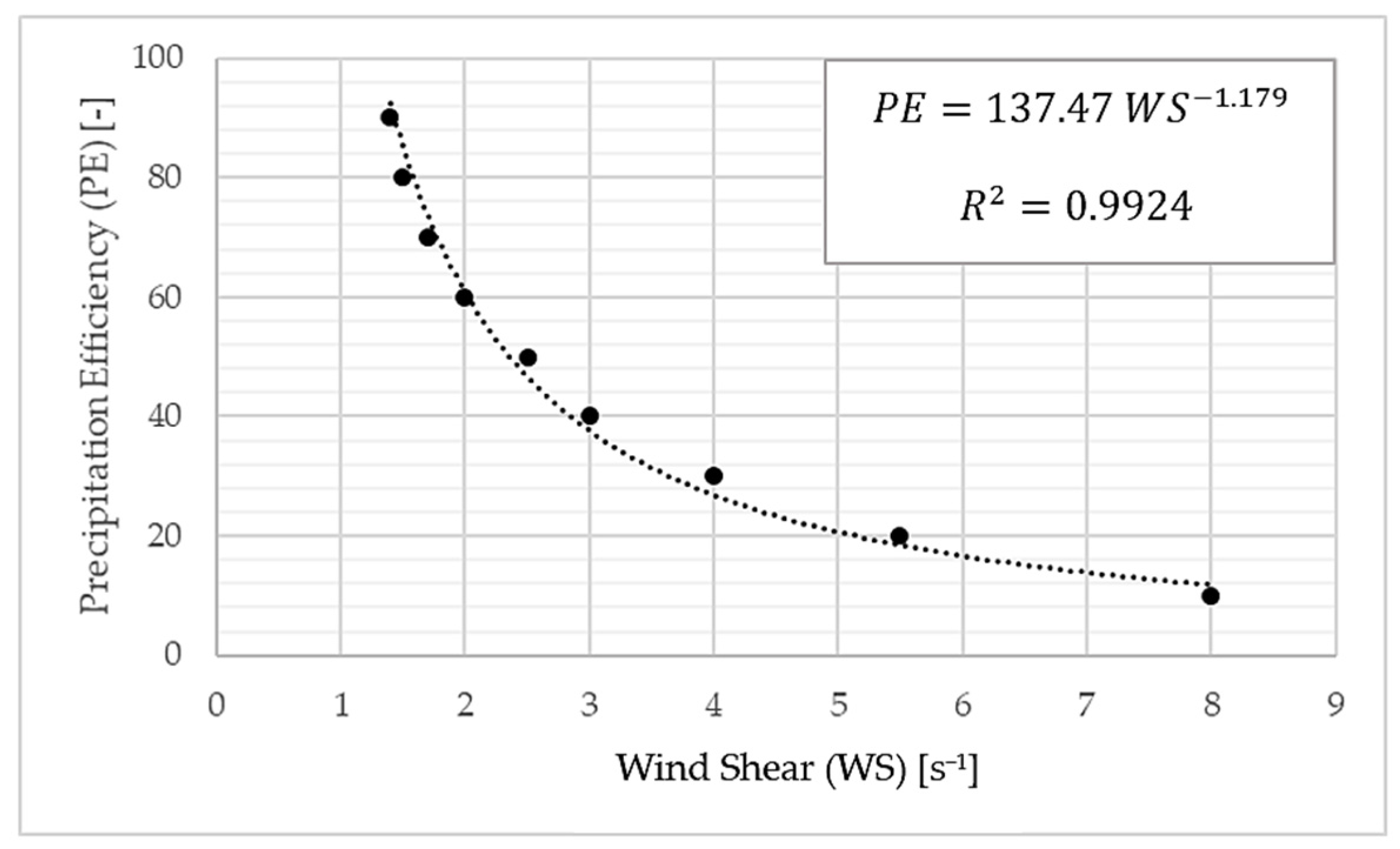
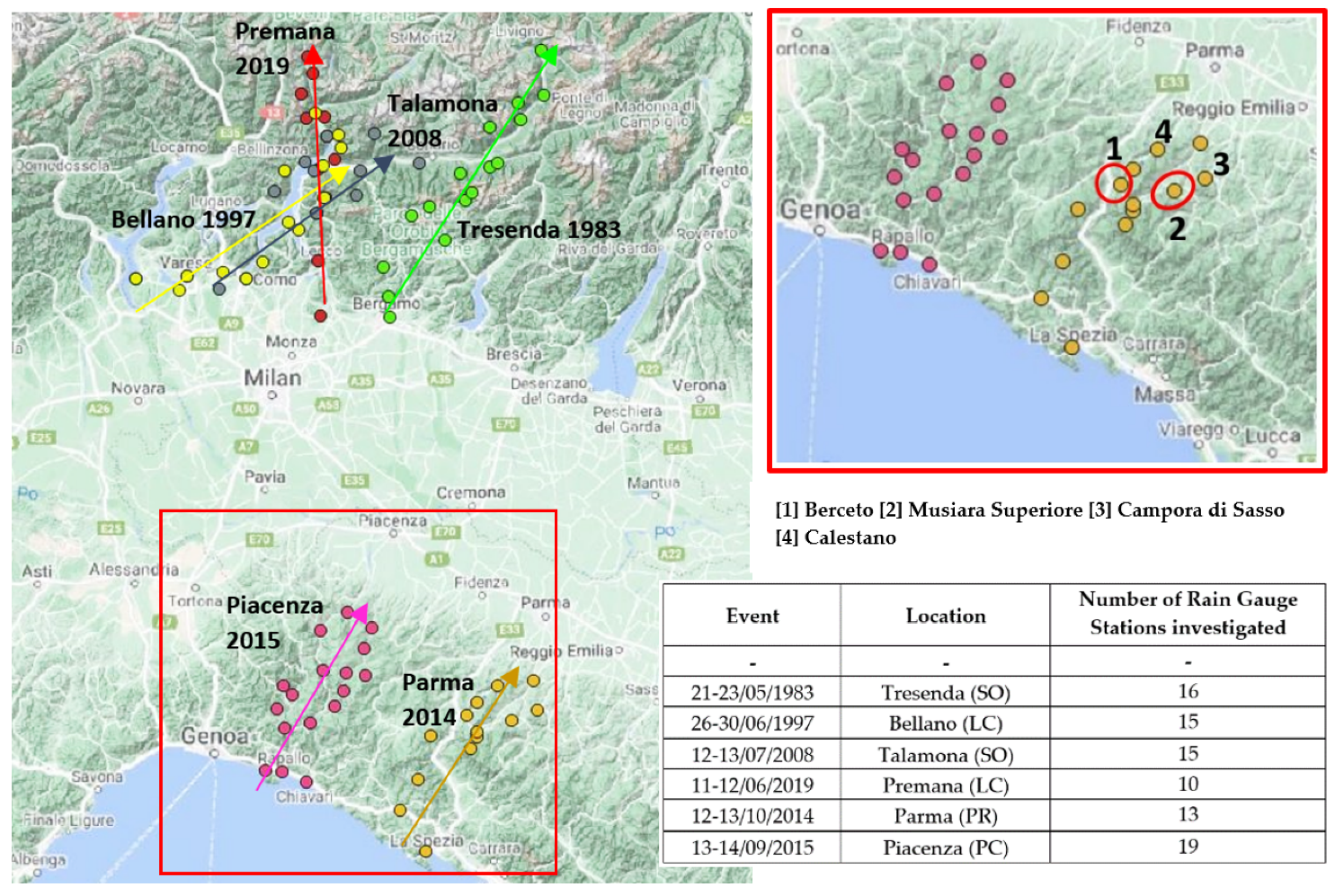
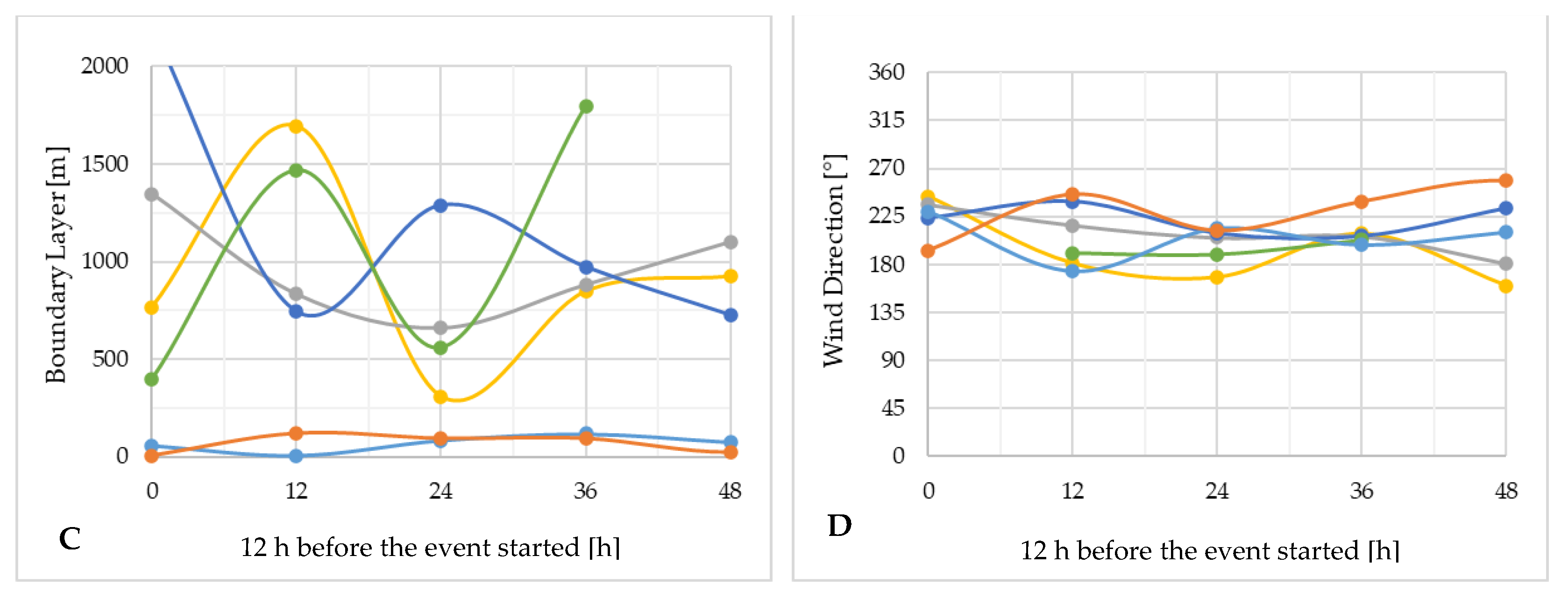
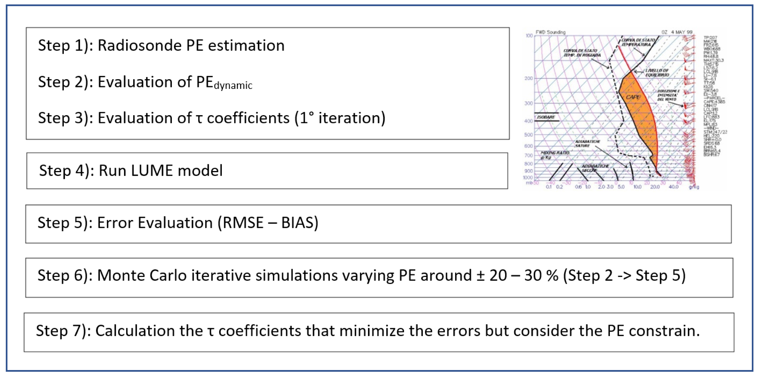
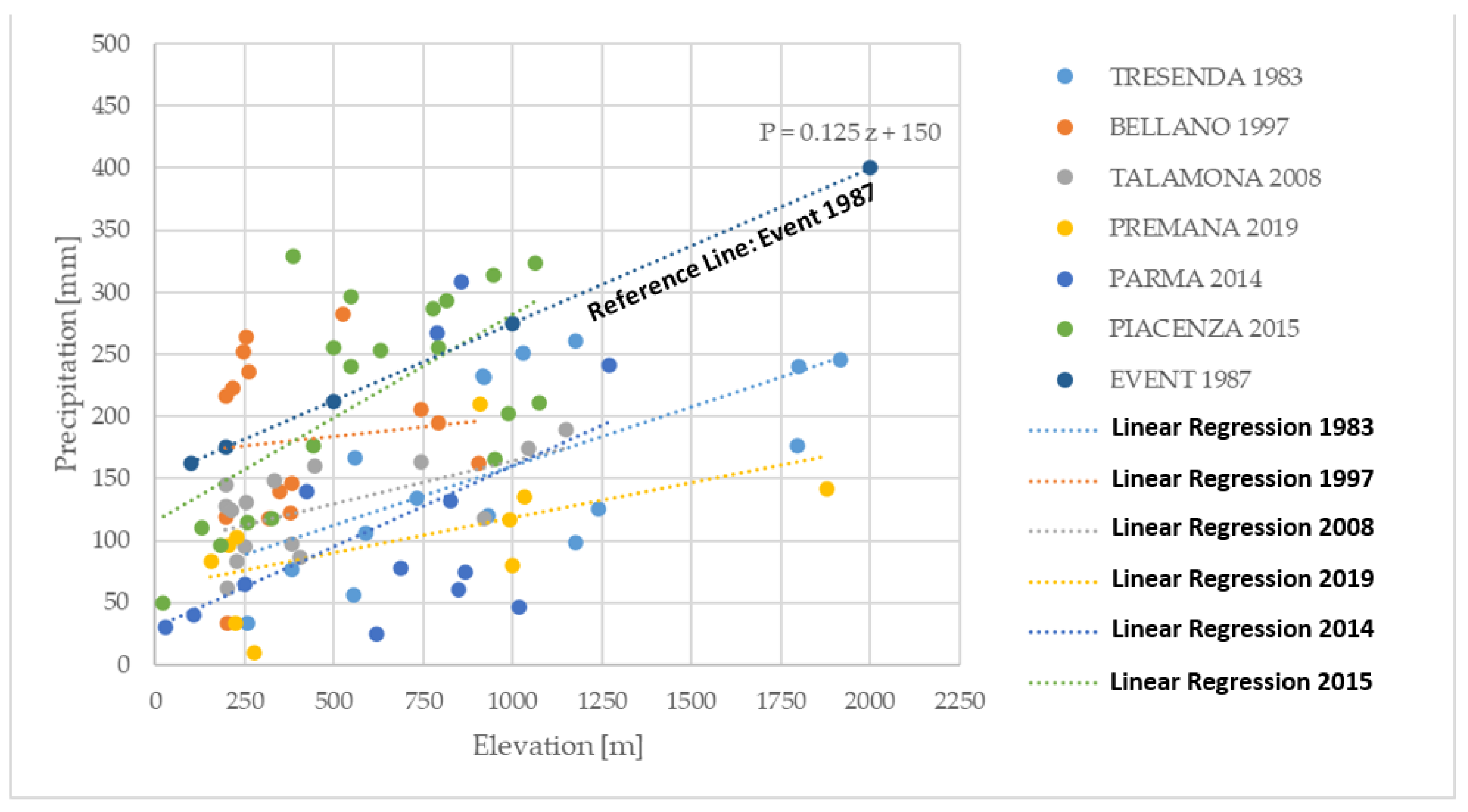
Table 1.
Definition of errors in LUME based on their possible propagation in additive or multiplicative error models.
Table 1.
Definition of errors in LUME based on their possible propagation in additive or multiplicative error models.
| Additive | Multiplicative | |
|---|---|---|
| Functional Form | ||
| Bias [mm] | ||
| Root Mean Square Error [mm] | ||
| All Indicator Scores (AIS) [mm] | ||
Table 2.
Studied events of extreme precipitation. Dates, locations, and extreme precipitation parameters that describe the maximum amount, the duration, and the return period, and the hydrogeological effects recorded on the territory. For 2008, 2014, and 2015 events, (**) represents the duration of the most intense phase, while () is the duration of the entire event.
| Event | Location | Station | Extreme Precipitation | Hydrogeological Effects | ||
|---|---|---|---|---|---|---|
| - | - | - | Max Amount (mm) | Duration (h) | Return Period (yr) | - |
| 21–23 May 1983 | Tresenda (SO) | Ponte di Ganda | 261 | 60 | ≈100 | Shallow landslides |
| 26–30 June 1997 | Bellano (LC) | Bellano | 283 | 96 | ≈50 | Flash floods |
| 12–13 July 2008 | Talamona (SO) | Morbegno | 60 (174) | 12 ** (72) | ≈2 (10) | Debris flows |
| 11–12 June 2019 | Premana (LC) | Premana | 209 | 13 | ≈200 | Flash floods |
| 12–13 October 2014 | Parma (PR) | Marra | 296.6 (298.8) | 8 ** (12) | ≈200 | Debris flows |
| 13–14 September 2015 | Piacenza (PC) | Salsominore | 307.4 (308.6) | 6 ** (12) | ≈200 | Debris flows |
Table 3.
LUME parameters for extreme precipitation modelling. For 2014 and 2015, due to the greater distance of the Ajaccio radiosonde station from the location of events (300 km), we also considered the Cuneo () and Linate [] radiosonde stations (150 km and 100 km) located downstream.
Table 3.
LUME parameters for extreme precipitation modelling. For 2014 and 2015, due to the greater distance of the Ajaccio radiosonde station from the location of events (300 km), we also considered the Cuneo () and Linate [] radiosonde stations (150 km and 100 km) located downstream.
| Event | Location | LUME Parameters for Each Extreme Precipitation Event | |||||||
|---|---|---|---|---|---|---|---|---|---|
| - | - | U (m s-1) | Dir (°) | Hw (m) | WVF0 max (kg m−1 s−1) | τc (s−1) | τf (s−1) | hBL (m) | Pbackground (mm) |
| 21–23 May 1983 | Tresenda (SO) | 18.6 | 192.4 | 2600 | 482.4 | 3750 | 500 | ≈600 | 34 |
| 26–30 June 1997 | Bellano (LC) | 20.8 | 196.4 | 2600 | 731.3 | 3500 | 750 | ≈400 | 76 |
| 12–13 July 2008 | Talamona (SO) | 15.8 | 222.3 | 2600 | 545.6 | 2500 | 1000 | ≈250 | 60 |
| 11–12 June 2019 | Premana (LC) | 22.2 | 194.3 | 2600 | 607.5 | 1000 | 500 | ≈600 | 10 |
| 12–13 October 2014 | Parma (PR) | 15.4 | 205.1 | 2600 | 832 (610) [600] | 1000 | 750 | ≈100 | 0 |
| 13–14 September 2015 | Piacenza (PC) | 15.9 | 229.2 | 2600 | 720 (640) [815] | 1300 | 1000 | ≈100 | 0 |
Table 4.
Error calculation in LUME for the event examined with the two error models. For the event of Parma 2014, two rain gauge stations (Berceto and Musiara Superiore) were excluded since they were suspected to be outliers or not representative of that event.
Table 4.
Error calculation in LUME for the event examined with the two error models. For the event of Parma 2014, two rain gauge stations (Berceto and Musiara Superiore) were excluded since they were suspected to be outliers or not representative of that event.
| Event | Location | BIAS (mm) | RMSE (mm) | AIS (mm) | ||
|---|---|---|---|---|---|---|
| - | - | Additive | Multiplicative | Additive | Multiplicative | - |
| 21–23 May 1983 | Tresenda (SO) | 7.9 | 2.05 | 29.42 | 35.92 | 75.29 [5] |
| 26–30 June 1997 | Bellano (LC) | −16.80 | −19.81 | 39.80 | 41.76 | 118.17 [6] |
| 12–13 July 2008 | Talamona (SO) | 4.9 | 5.09 | 30.81 | 29.79 | 70.59 [2] |
| 11–12 June 2019 | Premana (LC) | 4.31 | 2.92 | 19.78 | 19.42 | 46.43 [1] |
| 12–13 October 2014 | Parma (PR) | −3.76 | −0.2 | 33.36 | 47.07 | 84.35 [4] |
| 13–14 September 2015 | Piacenza (PC) | −4.43 | −3.4 | 32.24 | 48.93 | 89.05 [5] |
Table 5.
Linear regression coefficient and R2 calculated for the event simulated by LUME. Note the poor score of the regression, especially for the Bellano 1997 event, while for the others, the R2 is always somewhat below 0.5.
Table 5.
Linear regression coefficient and R2 calculated for the event simulated by LUME. Note the poor score of the regression, especially for the Bellano 1997 event, while for the others, the R2 is always somewhat below 0.5.
| Event | Location | Linear Regression Precipitation–Elevation Coefficients | ||
|---|---|---|---|---|
| - | - | a [mm m-1] | b [mm] | R2 |
| 21–23 May 1983 | Tresenda (SO) | 0.096 | 64.386 | 0.400 |
| 26–30 June 1997 | Bellano (LC) | 0.030 | 169.280 | 0.010 |
| 12–13 July 2008 | Talamona (SO) | 0.069 | 94.731 | 0.385 |
| 11–12 June 2019 | Premana (LC) | 0.057 | 61.786 | 0.322 |
| 12–13 October 2014 | Parma (PR) | 0.130 | 30.267 | 0.239 |
| 13–14 September 2015 | Piacenza (PC) | 0.167 | 115.240 | 0.410 |
| 16–19 July 1987 | Event 1987 | 0.125 | 150 | - |
Publisher’s Note: MDPI stays neutral with regard to jurisdictional claims in published maps and institutional affiliations. |
© 2022 by the authors. Licensee MDPI, Basel, Switzerland. This article is an open access article distributed under the terms and conditions of the Creative Commons Attribution (CC BY) license (https://creativecommons.org/licenses/by/4.0/).
Share and Cite
MDPI and ACS Style
Abbate, A.; Papini, M.; Longoni, L. Orographic Precipitation Extremes: An Application of LUME (Linear Upslope Model Extension) over the Alps and Apennines in Italy. Water 2022, 14, 2218. https://doi.org/10.3390/w14142218
AMA Style
Abbate A, Papini M, Longoni L. Orographic Precipitation Extremes: An Application of LUME (Linear Upslope Model Extension) over the Alps and Apennines in Italy. Water. 2022; 14(14):2218. https://doi.org/10.3390/w14142218
Chicago/Turabian StyleAbbate, Andrea, Monica Papini, and Laura Longoni. 2022. "Orographic Precipitation Extremes: An Application of LUME (Linear Upslope Model Extension) over the Alps and Apennines in Italy" Water 14, no. 14: 2218. https://doi.org/10.3390/w14142218
Note that from the first issue of 2016, this journal uses article numbers instead of page numbers. See further details here.