Redefining and Calculating the Pass-through Rate Coefficient of Nonpoint Source Pollutants at Different Spatial Scales

Abstract

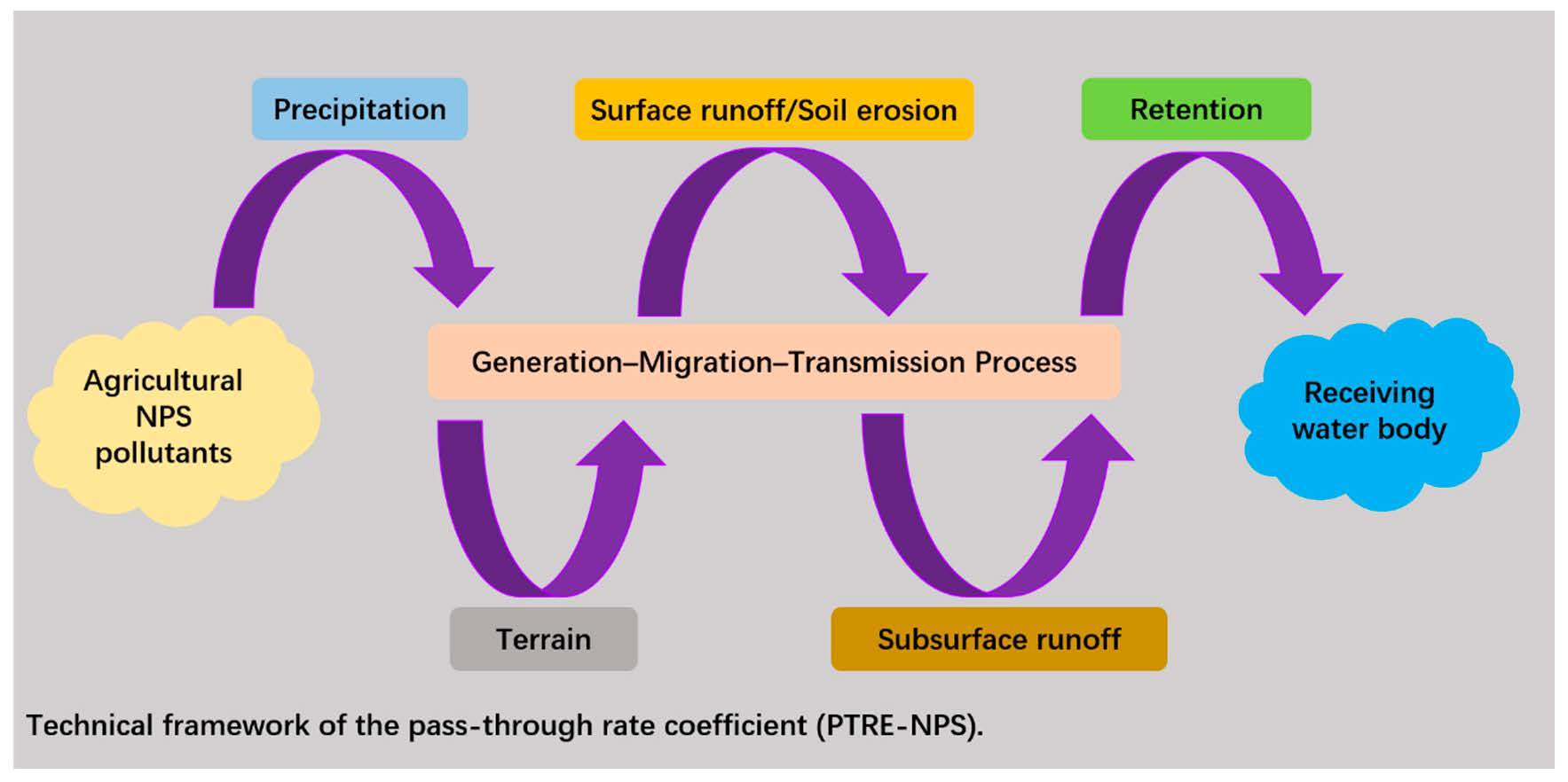
Accurately converting nonpoint source pollution loads from the watershed scale to administrative scale is challenging. A promising solution is calculating the pass-through rate coefficient of nonpoint source pollutants (PTRE–NPS) at the watershed scale and discretizing the watershed units on grids with the same area but with different PTRE–NPS information. However, the pollution load of agricultural nonpoint sources has received far more attention than the PTRE–NPS. Moreover, as most of the existing PTRE–NPS results are obtained by distributed, semi-distributed models and the field monitoring of small watersheds, they are not easily extended to the national-scale management of nonpoint source pollution. The present study proposes a new conception of PTRE-NPS and tests it on different spatial scales by a coupled model, which captures the entry of agricultural nonpoint source pollutants into rivers and lakes. The framework includes five major modules: a pollutant driving and loss module, a surface runoff module, a soil erosion module, a subsurface runoff module, and a retention module. The model was applied in simulations of agricultural nonpoint source pollution in the Hongfenghu reservoir watershed with a karst hydro-geomorphology, which exists in the mountainous region of southwest China. On the watershed scale, the PTRE–NPS of total nitrogen (TN) and total phosphorous (TP) ranged from 0 to 2.62 (average = 0.18) and from 0 to 3.44 (average = 0.19), respectively. On the administrative scale, the PTRE–NPS of TN and TP were highest in Baiyun Town. The TN and TP loads of the agricultural nonpoint source pollution in the rivers and lakes of the Hongfenghu reservoir watershed were 1707.78 and 209.03 t, respectively, with relative errors of −45.36% and 13.07%, respectively. Most importantly, the developed framework can scientifically represent the generation–migration–transmission process of agricultural nonpoint source pollutions in each grid at both the watershed and administrative scales.

1. Introduction

In recent years, agricultural nonpoint source pollution (NPS) has gradually become the main pollution source of water environments in many countries and regions [1]. According to the Second National Census on Source of Pollution of China, the total nitrogen (TN) and total phosphorus (TP) emissions accounted for 304.14 and 31.54 million tons of natural pollutants, respectively, in 2017. Most of the TN and TP [141.49 (46.52%) and 21.20 million tons (67.22%), respectively] are sourced from agricultural activities [2]. Therefore, agricultural source pollutants are important causes of environmental pollution in water bodies and have raised the concern of the Chinese government. In 2018, the supervision and guidance of agricultural NPS control became an important function of the Ministry of Ecology and Environment of the People’s Republic of China. Since the 1980s, research on agricultural NPS has increased in China and includes load calculation, management practices, and model construction [3,4,5,6,7,8,9]. However, the accurate conversion of NPS loads from the watershed scale to the administrative scale remains an ongoing national challenge.

Accurately estimating the impact of agricultural NPS on environmental water quality is necessary for scientific decision-making and effective control measures. Calculations of agricultural NPS loads require knowledge of the pollution source activities, production and discharge coefficients, and the pass-through rate coefficient of NPS (PTRE–NPS). The first two data are obtained by on-site monitoring or field investigation, but the PTRE–NPS is affected by various factors, and is limited by financial, human activities, and material support for field monitoring. The production and discharge coefficients, export coefficient, and PTRE–NPS are widely variable. The production coefficient of livestock and poultry under normal production and management conditions is determined from the amounts of primary pollutants produced by the pollution source during a certain period. The discharge coefficient under typical normal production and management conditions is also determined from the amount of pollutants emitted by individual livestock and poultry within a certain time period, but is determined after reduction by the treatment facility or (if untreated) after direct discharge into the environment. The export coefficient expresses the rate at which nitrogen or phosphorus is exported from each land-use type in the catchment [10]. The production, discharge, and export coefficients are given for the different agricultural pollution sources in different scales (administrative scale for the production and discharge coefficients, watershed scale for the export coefficient). However, a single agricultural pollution source has a large spatial heterogeneity under different conditions, being influenced by regional location, hydrology, meteorology, and the underlying surface conditions. Neither the production and discharge coefficients nor the export coefficient is sufficient for characterizing the impact of agricultural NPS into rivers and lakes, which is needed for estimating NPS loads. Furthermore, directly multiplying the export coefficient at the watershed scale with the coefficient of production and discharge coefficient and the activity level of pollution sources at the administrative scale will increase the error of the results. Consequently, the calculation results are not accurate enough, and the impacts of other important pollution sources into rivers and lakes are obscured. As agricultural NPS are diverse and follow a complex migration process, they may not affect the rivers and lakes in all spatial regions. Factors such as rainfall, topography, surface runoff, underground storage, leaching, and plant retention also play a role [11]. The pollutants will aggregate in a certain space and form a transport channel. Pollutants not entering the transport channel will not necessarily affect rivers and lakes. Accordingly, the PTRE–NPS expresses the ratio of pollutant load in the main channel of the corresponding sub-basin (which has been driven, transmitted, and intercepted by rainfall and the underlying surface media) to pollutant production. The PTRE–NPS reflects the natural reduction process of pollutants on the land surface and excludes the natural purification process of rivers and lakes.

At present, the loads of agricultural NPS are estimated by both field monitoring and model simulations. The models can be empirical or mechanistic. Empirical models are based on theoretical concepts such as nutrient balance, risk assessment, and export coefficients. Examples are the export coefficient model (ECM) and phosphorus index (PI) [12,13,14]. Mechanistic models couple the data of hydrology, meteorology, land use, and soil type, and characterize the entry processes of pollutants into rivers and lakes, namely, flow generation, evapotranspiration, soil erosion, soil flow, and channel transmission. The Annualized Agricultural Nonpoint Source Pollution (AnnAGNPS), Soil & Water Assessment Tool (SWAT), and the Hydrological Simulation Program FORTRAN (HSPF) have all been successfully applied to agricultural NPS calculations in mesoscale areas [15,16,17]. However, both empirical and mechanistic models have some limitations (

Table 1. Comparison of models for simulating agricultural nonpoint source pollution.

Type	Model	Output	Factor					Reference
			Correction of Production and Discharge Coefficient	Difference of Spatial Distribution of Precipitation	Difference of Spatial Distribution of Terrain	Difference of Transmission Process	Plants Retention
Empirical model	USLE	Raster	×	√	√	√	×	[18,19,20]
	$\alpha ={\alpha }_i\times {\alpha }_s=\frac{f\left(r_i\right)}{f\left(\overline{r}\right)}\times \frac{f\left(R_j\right)}{f\left(\overline{R}\right)}$	Raster	√	√	×	×	×	[21]
	$\beta =\frac{L\left(\overline{{\theta }_i}\right)}{L\left(\overline{{\theta }_d}\right)}=\frac{c{\overline{\theta }}_l{}^d}{c{\overline{\theta }}_d{}^d}=\frac{{\overline{\theta }}_l{}^d}{{\overline{\theta }}_d{}^d}$	Raster	√	×	√	×	×	[21,22]
	SCS–CN	Raster	×	×	×	√	×	[23,24]
	VSA–CN	Raster	×	×	×	√	×	[23,24]
	$LI=\frac{{\left[P_{annual}-0.4\left(\frac{25400}{CN}-254\right)\right]}^2}{P_{annual}+0.6\left(\frac{25400}{CN}-254\right)}\times \sqrt[3]{2\times \frac{P_{dry}}{P_{annual}}}$	Raster	×	×	×	√	×	[25,26]
	$RI=\ln \left(\frac{{{\displaystyle \sum }}_{DA=1}^N{T}_{DAi}}{\tan B_{DAi}}\right)$	Raster	×	×	×	×	√	[27]
Mechanism model	SWAT	HRUs	×	√	√	√	×	[15]
	AnnAGNPS	Small watershed	×	√	√	√	×	[16]
	HSPF	Small watershed	×	√	√	√	×	[17]

): for empirical models, the pollutant transport process before pollutants enter the river is regarded as a “black box system”, the process of subsurface runoff is not considered enough, and the accuracy is generally lower than the mechanistic model and field monitoring; mechanistic models demand a large volume of monitoring data and need a long time for operation. Modern technology based on raster data, which accounts for spatial transformations, has a natural advantage in error reduction, especially at national scales. To calculate scientifically accurate actual loads, the transport mechanism of nonpoint source pollutants from source to sink should be considered.

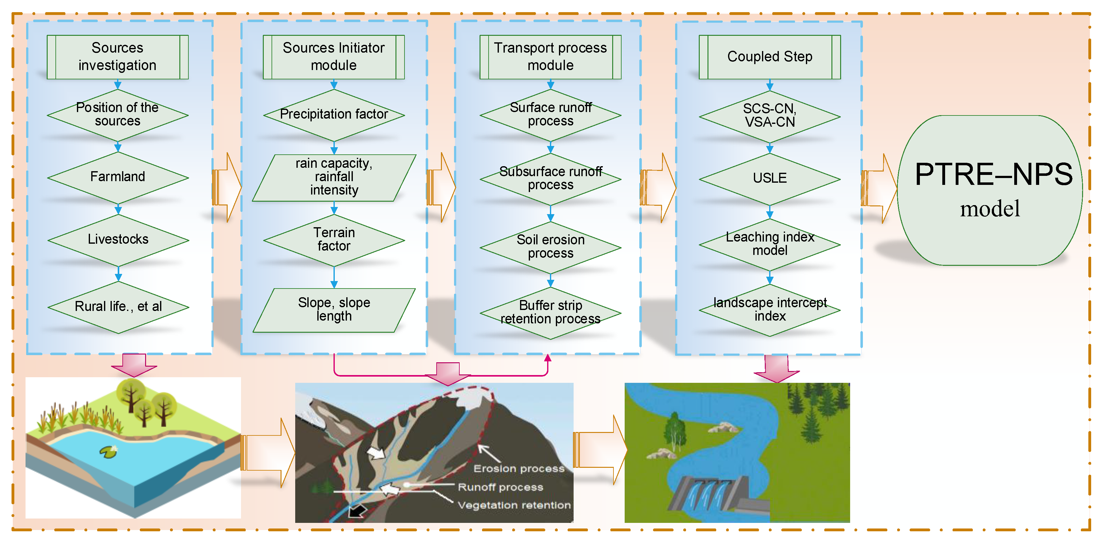
The entry of agricultural NPS into rivers and lakes is driven by precipitation and topography. The pollutants enter the transportation channel with surface runoff, soil erosion, soil leaching, and groundwater runoff and are finally intercepted by forest and grass before entering the receiving water bodies. To capture this complex process, this study proposes a coupled PTRE–NPS model with five modules: a rainfall module, a terrain module, a transportation module, a leaching module, and a retention module. The transportation mechanism of pollutants has been widely researched [18,19,20,21,22,23,24,25,26,27,28,29,30,31,32,33]. Agricultural NPS are affected by the spatial distribution of rainfall and can vary with different rainfalls in different regions in the same year [21,22]. Depending on the rainfall conditions and water holding capacity of the soil, the runoff yield occurs under two mechanisms: infiltration excess runoff or saturation excess runoff. These processes can be modeled by the Soil Conservation Service—Curve Number (SCS–CN) and Variable Source Area—Curve Number (VSA–CN), respectively [34,35]. The SCS–CN model is widely used for predicting event-based rainfall surface runoff and its processes. This model is advantaged by few parameters, a simple calculation process, and easily acquired data, but is limited to surface runoff simulations under the excess infiltration mechanism of runoff yield. Pollutant transportation is also affected by the soil infiltration capacity, which affects the migration of pollutants through a soil profile. Regardless of the influence of groundwater and base flow, the soil infiltration capacity and pollutant load intensity can approximate the actual infiltration capacity [25,26,36]. In contrast, pollutants transported into rivers and lakes are more influenced by the transmission distance, the presence of forest and grass, and the surface buffer system [27]. A larger distance between the pollution source and the receiving rivers and lakes is associated with wider interception bands, smaller slopes, and higher interception efficiency.

To overcome these weaknesses and to fully leverage the advantages of the existing methods for PTRE–NPS, two hypotheses were proposed. First, it is possible to generalize the major process of transfer of pollutants from sources to sinks; second, the generalized process can be integrated into a new model on the watershed and administrative scales. In this study, the PTRE–NPS model is developed, which is based on the transport mechanism of pollutants, considers the diversity of agricultural NPS, complexity of spatial transportation, and regional differences. The reliability of the PTRE-NPS model is conducted in the Hongfenghu reservoir watershed in Guiyang and Anshun Cities of Guizhou Province in southwest China. Overall, the major purpose of this study is to establish the simple model to predict the path-through rate of NPS pollutants based on the grid, and to reduce the errors of pollution loads between the watershed and administrative scales, by which planners can prioritize high-risk areas of agricultural NPS.

2. Materials and Methods

2.1. Study Area

The Hongfenghu reservoir watershed is located southwest of Guiyang City and northeast of Anshun City in Guizhou Province of China. The geographical location is 106°00′ E–106°30′ E and 26°10′ N–26°30′ N. The landform is a low karst hill with a gentle slope. The annual average precipitation is 1271.95 mm, concentrated in May to October. The 1126.6 km² area includes Pingba County, Huaxi District, Xixiu District, and Qingzhen City, with a total of 16 villages and towns (Figure 1). As an important source of surface drinking water in Guiyang, the reservoir water is of a medium nutrition type and is clearly trending toward eutrophication. The main supplementary water source is the Yangchanghe watershed in the upper reaches of the site. The Hongfenghu reservoir watershed is polluted with small amounts of NPS, mainly contributed by agricultural activities. The industrial structure is mainly agricultural planting and animal husbandry, which typify agricultural farming areas. Therefore, reversing the water eutrophication trend and ensuring the normal water supply function are of high practical significance.

2.2. Data Source

The input database included the Digital Elevation Model (DEM), land use, soil types, vegetation map, streams, and boundaries of the study area. The meteorological data, hydro-water data, and socioeconomic data were also used. The slope of the study area was calculated by using the surface analysis module of ArcGIS based on DEM data. The details are given in

Table 2. Data used in the current research.

Data	Storage	Map Scale	Data Precision	Period
Digital Elevation Model	Grid	1:50,000	30 × 30 m	2013
Land use	Shp	1:100,000	30 × 30 m	2013
Soil type	Shp	1:1000,000		2010
Vegetation coverage	Grid	1:1000,000	1000 × 1000 m	2016
Stream	Shp	1:250,000		2013
Administrative boundary	Shp	1:250,000		2013
Meteorological data	*.txt and *.xls	—	Daily	2013
Hydrological and water quality data	*.txt and *.xls	—	Huangmao village	2013
Socioeconomic data	*.txt and *.xls	—	Years	2013

.

2.3. Methodology

Considering the effects of precipitation, terrain, surface runoff, leaching, and retention on NPS pollution, the coupled model included the sources initiator module and transport process module (Figure 2); the PTRE-NPS for TN and TP are described as follows:

$${\lambda }_{TN}={\alpha }_{TN}\ast \beta \ast TI\ast LI\ast R{I}_{TN}$$

(1)

$${\lambda }_{TP}={\alpha }_{TP}\ast \beta \ast \left(\mathrm{a}\ast TI+b\ast USLE\right)\ast LI\ast R{I}_{TP}$$

(2)

In these expressions, ${\alpha }_{TN}$ and ${\alpha }_{TP}$ are the rainfall modules of TN and TP, respectively; $\beta$ is the terrain module; TI and LI are the transportation and leaching indices, respectively; and RI_TN and RI_TP are the retention indices of TP and TN, respectively. The Universal Soil Loss Equation (USLE) is the soil erosion module, and a and b are the percentages of dissolved and particulate phosphorus, respectively.

2.3.1. The Sources Initiator Module

Considering the effect of the nonuniformities of precipitation and terrain on agricultural nonpoint source pollution, the purpose of the sources initiator module is to modify the export coefficient of each source located in a different position, which include the precipitation (α) and terrain (β) factors.

The precipitation factor α is determined by two aspects: the first is the temporal unevenness factor, and the second is the spatial unevenness factor. The precipitation factor α is described below.

$$\alpha =\frac{f\left(r_{annual}\right)}{f\left(r_{average}\right)}\times \frac{R_{annual}}{R_{average}}$$

(3)

where $f\left(r_{annual}\right)$ and $f\left(r_{average}\right)$ are the annual and multi-annual average pollutant flux determined by multiplying the water quality and runoff from the outlet of watershed.

The terrain factor (β) is used to describe the effect of terrain heterogeneity on the export coefficient of each source located in a different position. The terrain factor (β) is defined as:

$$\beta =\frac{f\left(slop{e}_i\right)}{f\left(slop{e}_{average}\right)}$$

(4)

where $f\left(slop{e}_i\right)$ and $f\left(slop{e}_{average}\right)$ are the pollutant flux from the grid cell i (30 m × 30 m) and the average pollutant flux in the watershed. Considering the terrain is not going to change significantly in short time periods, the terrain factor (β) just varies as the grid cell changes.

2.3.2. The Transport Process Modules

The transport process modules include four aspects: surface runoff, subsurface runoff, soil erosion, and buffer strip retention. The Soil Conservation Services—Curve Number method (soil conservation service curve number, SCS-CN) was used for the calculation of the runoff index [37], while the VSA-CN was used as the engine to calculate the subsurface runoff [38], and the USLE equation was used to calculate the soil erosion [18]. The buffer strip retention (RI) is defined as follows.

$$RI=\ln \left({\displaystyle \sum _{i=1}^n\frac{V_i·W_i}{\tan {\epsilon }_i}}\right)$$

(5)

where W_i is the width of the buffer strip at the downstream of each grid; ε is the slope of the buffer strip; V_i is the manning coefficient; n is the total amount of grids in watershed.

To unify the calculation unit, the results of the module data were standardized [27] as follows:

$$\mathrm{Normal} \mathrm{distribution}: N{X}_i=\frac{X-\min \left(X\right)}{\max \left(X\right)-\min \left(X\right)}$$

(6)

$$\mathrm{Skew} \mathrm{distribution}: N{X}_i=\frac{\phi X_i}{X_i} \mathrm{or} N{X}_i=\frac{X_i}{\phi X_i}$$

(7)

Here, NX_i is the standardized result; X are the actual values on each grid (1 km × 1 km); min (X) and max (X) are the minimum and maximum values, respectively, of the basic measuring unit in a typical watershed; φX_i is the median value of module i; and X_i is the grid value of module i.

To measure the loads of agricultural NPS entering rivers and lakes, the PTRE–NPS was first calculated at the watershed and administrative scales using the spatial weighted average method with ArcGIS 10.2. Second, the PTRE–NPS on the administrative scale was multiplied by the total amount of agricultural source pollutants discharged by the administrative division. The result, L, gives the amount of agricultural source pollutants entering rivers and lakes at the administrative division:

$$L=\left({\lambda }_1{f}_1+{\lambda }_2{f}_2+\cdots +{\lambda }_n{f}_n\right)\times S,$$

(8)

where n is the number of grids in the administrative division; λ_n is the PTRE–NPS in the nth grid unit; and S denotes the total emissions of the pollutants from agricultural sources in the given administrative district, such as the planting industry and livestock and poultry breeding industry, and scattered living in rural areas. f_i denotes the weight coefficient of the ith grid unit under the jurisdiction of a certain administrative division, which accounts for the area proportion of the given administrative division.

3. Results and Discussion

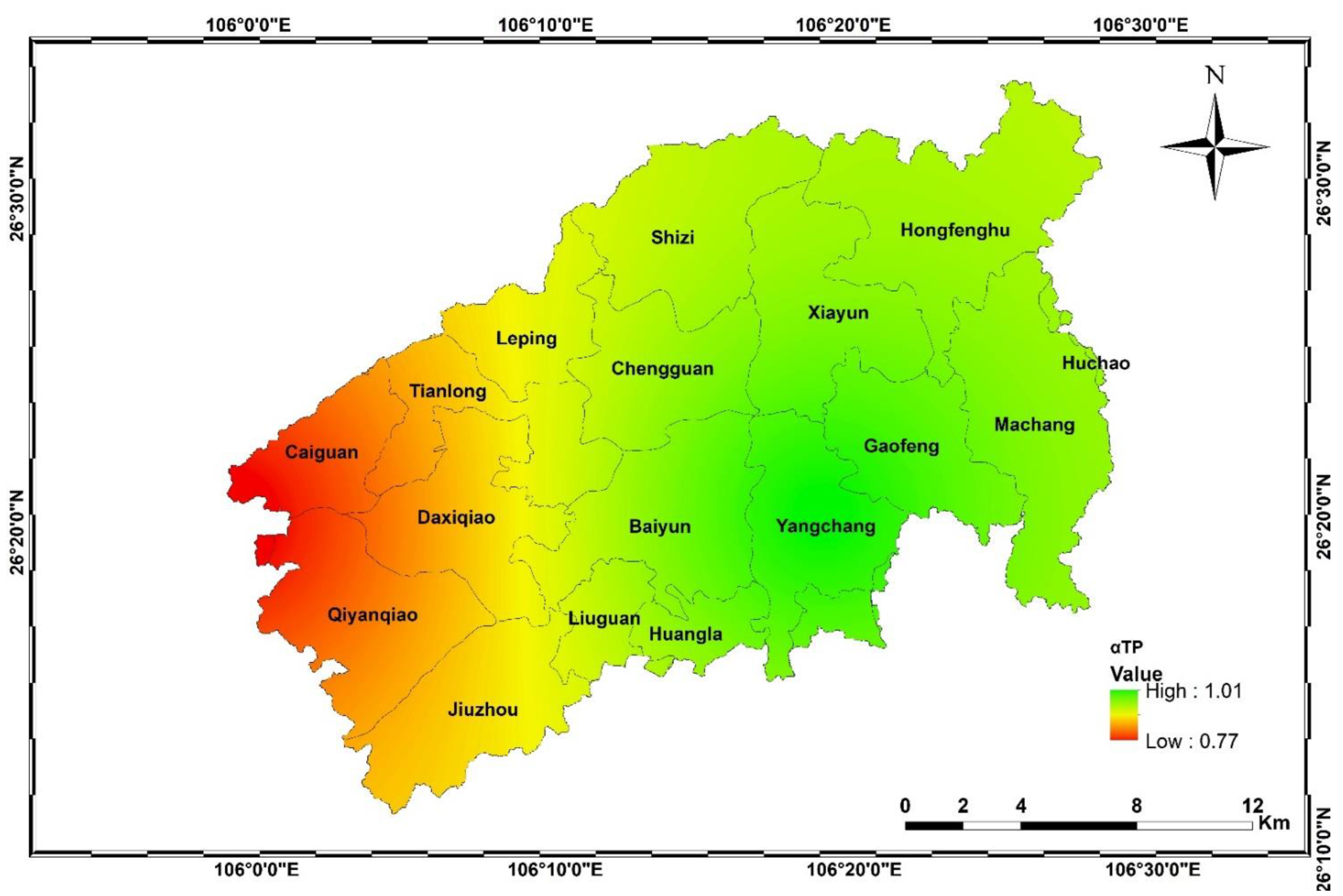
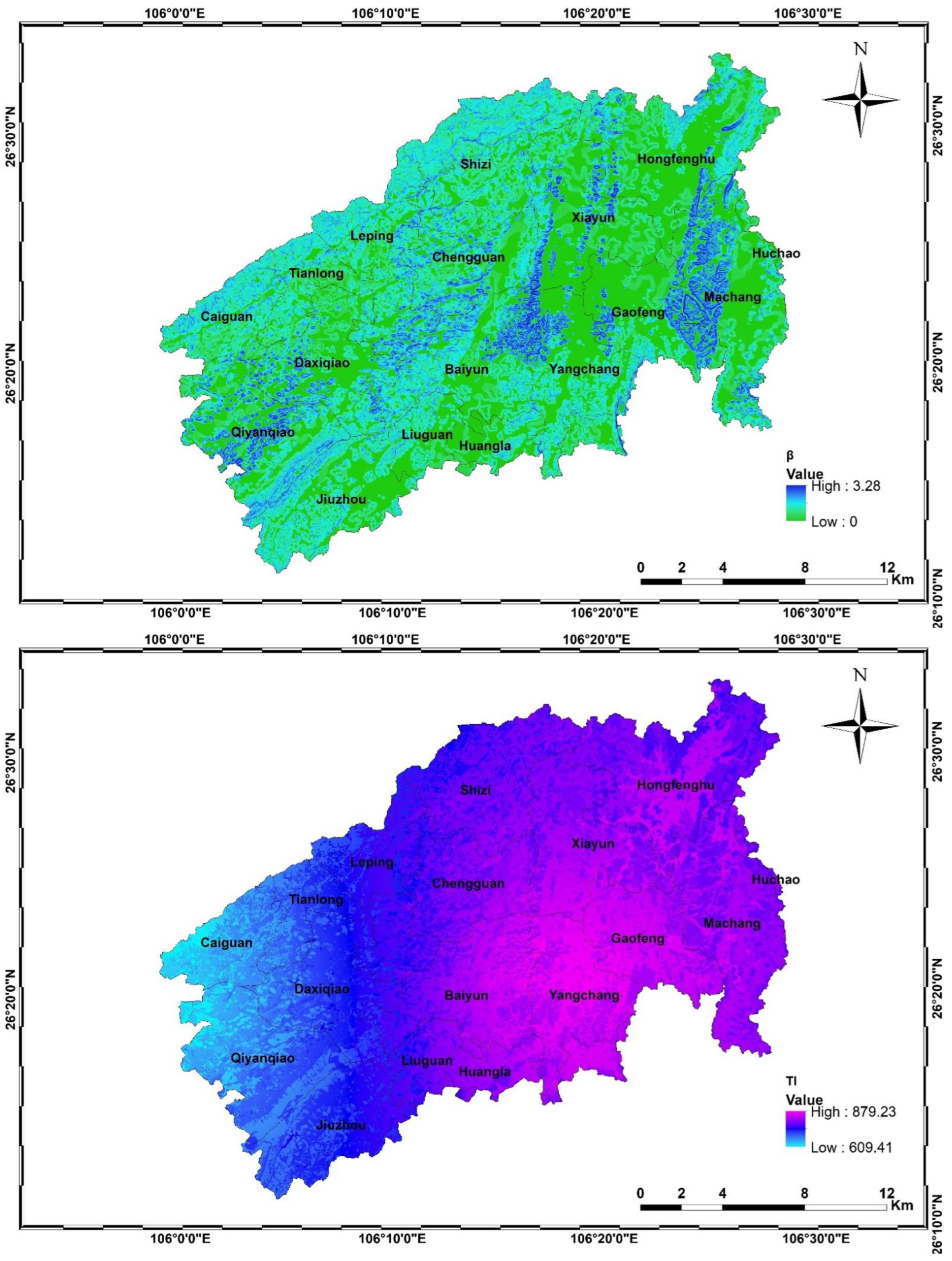
3.1. Spatial Distribution of Major Parameters of the PTRE-NPS

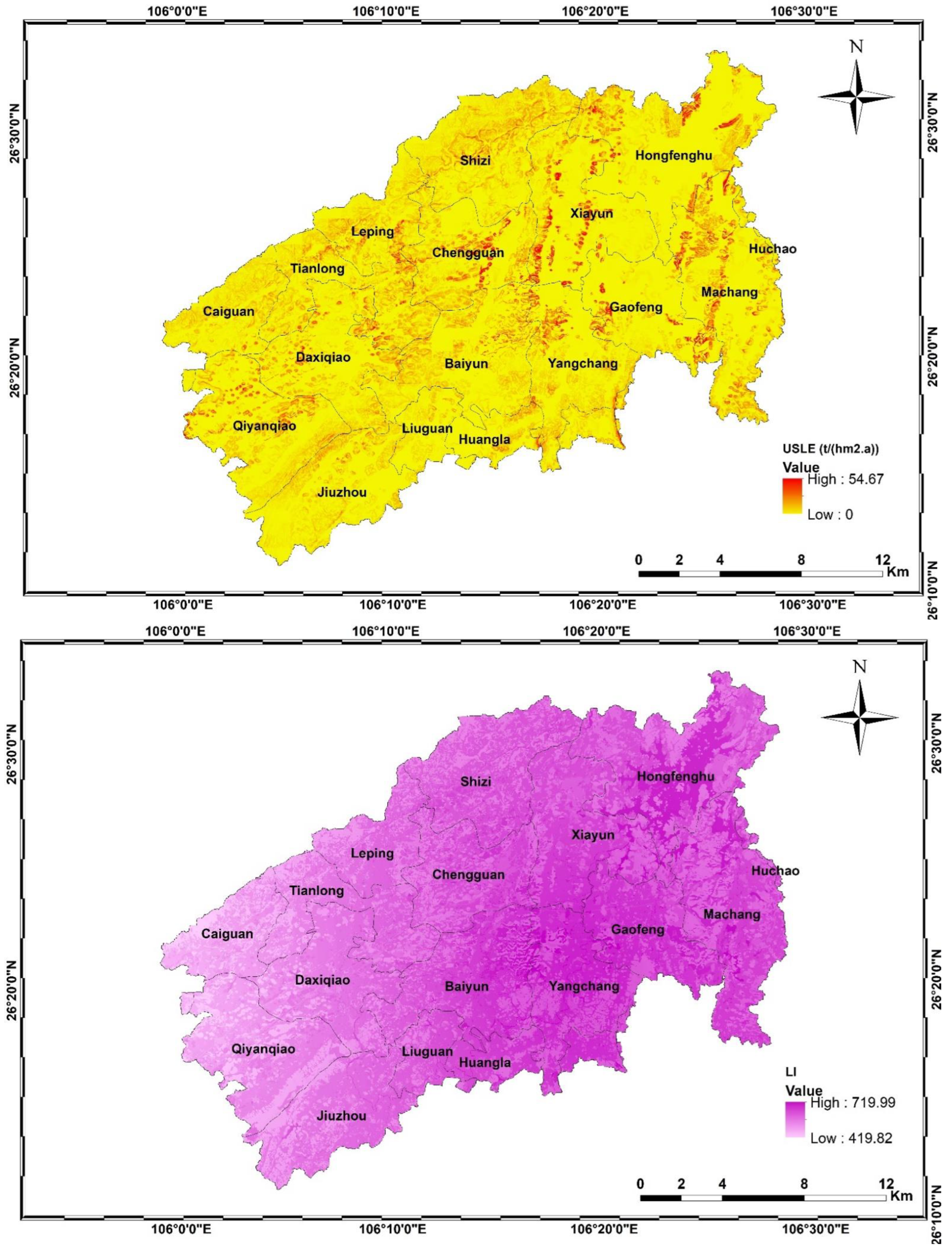
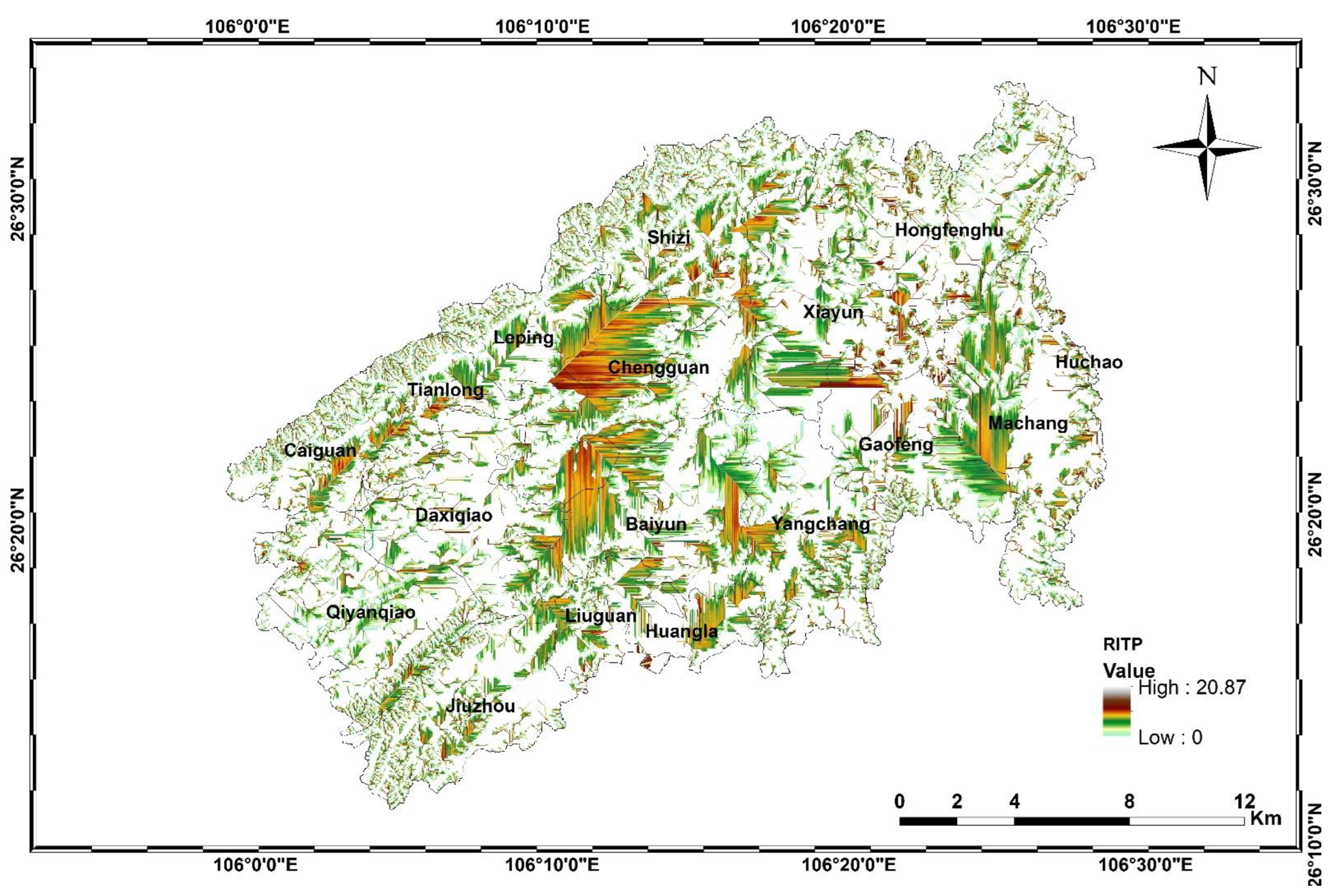
The spatial distribution of major parameters of the PTRE-NPS of TN and TP were performed (Figure 3 and Figure 4). The results show that α_TN and α_TP ranged from 0.74 to 0.97 and 0.77 to 1.01, respectively. β, LI, and TI of TN and TP were 0 to 3.28, 609.41 to 879.23 mm, and 419.82 to 719.99 mm, respectively. RI_TN and RI_TP were 0 to 20.41 and 0 to 20.87. From the perspective of the spatial distribution of rainfall, α, TI, and LI had high spatial similarity; the towns with high rainfall (Yangchang, Gaofeng, Baiyun) also had high α, TI, and LI, because these three indexes were mainly calculated based on rainfall. According to the spatial distribution of slope, β was proportional to the watershed slope, showing a high trend in the east. From the perspective of the land-use map, LI in the cultivated land was higher than other types of land use, which is likely because the CN value of cultivated land was larger than others. The spatial distribution of LI was similar to TI. The spatial distribution of RI_TN demonstrated that the smaller the slope was, the higher the vegetation coverage was, the higher interception efficiency would be, RI_TP was the same.

3.2. Spatial Distribution of PTRE–NPS on the Watershed and Town Scale

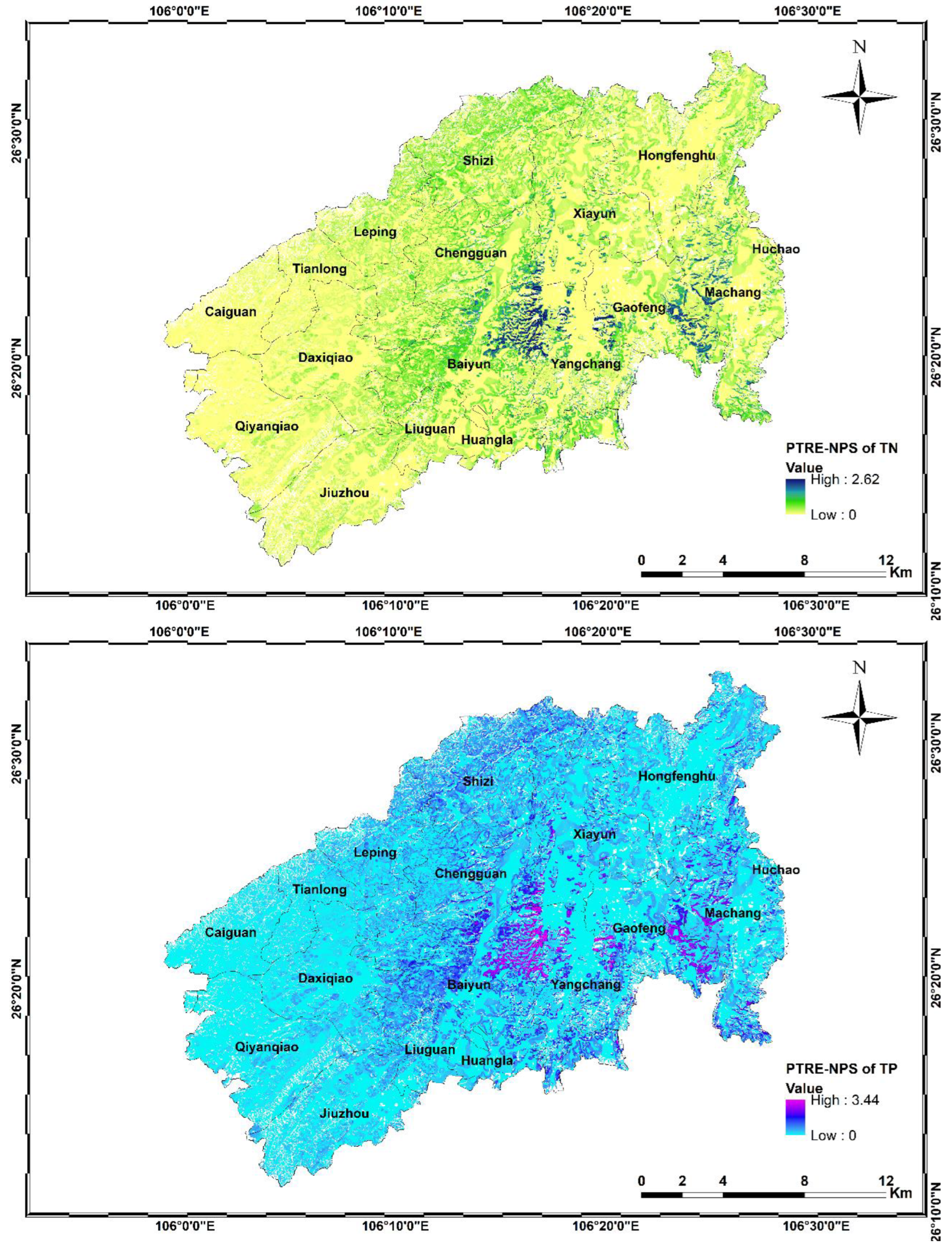
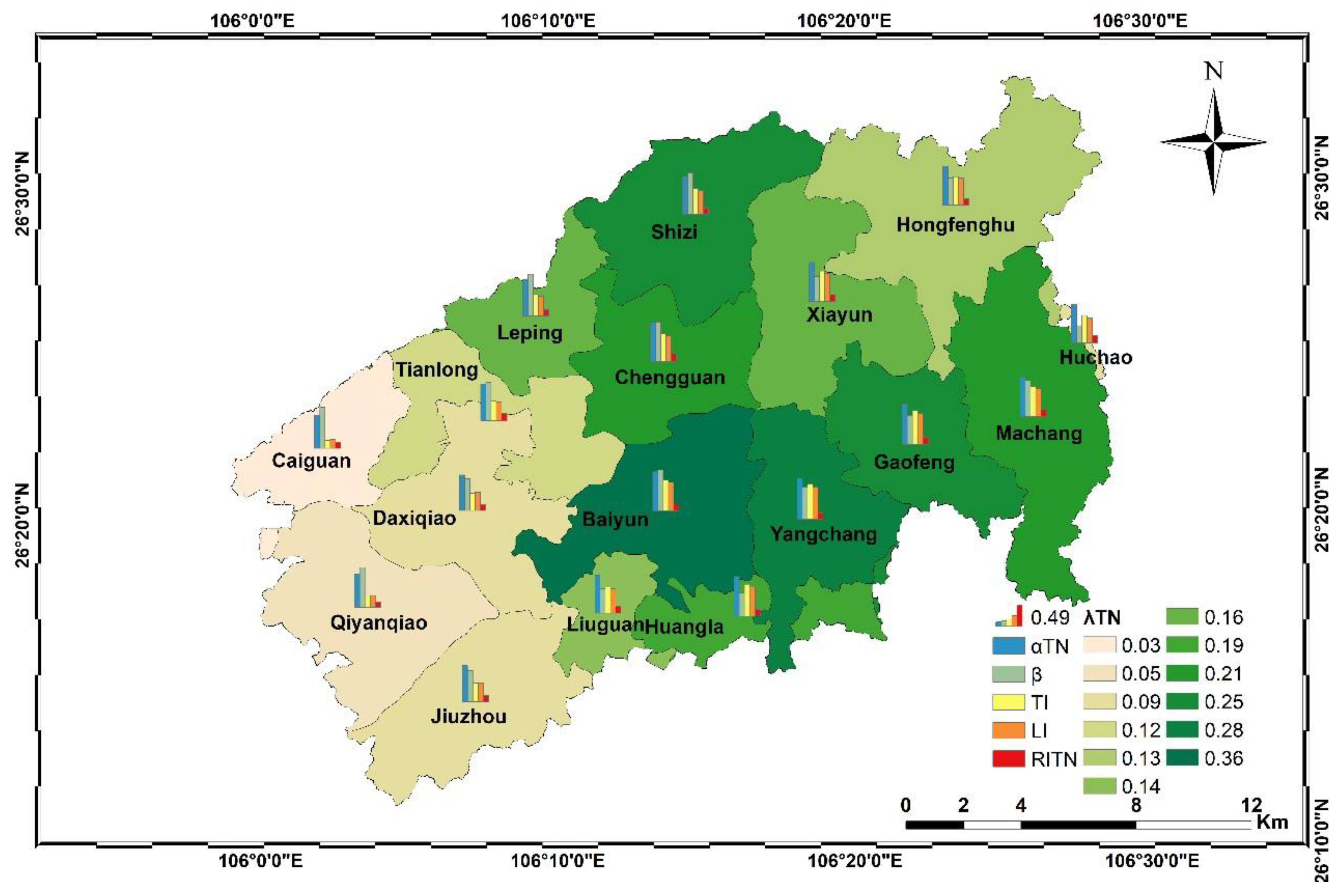
Figure 5 shows the spatial distributions of TN and TP in the Hongfenghu reservoir watershed at the watershed scale. The PTRE–NPS of the TN and TP ranged from 0 to 2.62 (average = 0.18) and 0 to 3.44 (average = 0.19), respectively. After obtaining the PTRE–NPS of the TN and TP of each grid in the township, the data distributions were assessed as normal or skewed. The skewed and normal data were represented by their averages and medians, respectively. Figure 6 and Figure 7 show the spatial distribution of PTRE-NPS of TN and TP at the town scale. The PTRE–NPS of TN in the townships ranged from 0.03 to 0.36, and those of the TP ranged from 0.04 to 0.39. The PTRE–NPS of both TN and TP were highest in Baiyun Town. It is likely because the terrain of Baiyun is higher, with a larger average slope; therefore, the flow is rapid and easy to cause the loss of nutrients in the occurrence of heavy rainfall.

3.3. Estimated Pollutants into the River from Agricultural Sources

Based on the First National Pollution Source Survey and early research in the study area, the TN and TP loads from the agricultural NPS in the Hongfenghu reservoir watershed were calculated by Equation (8) (

Table 3. TN and TP loads from agricultural NPS into the rivers and lakes of the Hongfenghu reservoir watershed.

Agricultural Source	TN (t)	Percent (%)	TP (t)	Percent (%)
Rural population	282.63	16.55	27.69	13.25
Livestock and poultry	384.79	22.53	99.70	47.69
Cultivated land	1040.36	60.92	81.65	39.06
Total	1707.78	100	209.03	100

). The TN load into the rivers and lakes was 1707.78 t, of which 282.63 t was attributed to the rural population, 384.79 t was attributed to livestock and poultry, and 1040.36 t was attributed to cultivated land. Among all of the pollution sources, cultivated land was the major contributor (accounting for 60.92% of TN loads), mainly owing to the unreasonable fertilizer rate and frequent cultivation activities. The TP loads into rivers and lakes were 209.03 t, of which 27.69, 99.70, and 81.65 t were contributed by the rural population, livestock and poultry, and cultivated land, respectively. Livestock and poultry was the primary contributor (accounting for 47.69% of TP loads), because of the improper management of animal feed and livestock manure.

3.4. Identification of Critical Source Areas

A comprehensive analysis of the distribution of TN and TP loads were performed, and the critical source areas (CSA) with high risks of NPS pollution were identified (Figure 8). Among the townships in the study area, Baiyun, Shizi, Yangchang, Chengguan, and Machang were mainly responsible for the TN loads from agricultural NPS, collectively contributing 56.73% of the TN loads (Figure 6). Baiyun, Shizi, and Chengguan also largely contributed to the TP loads from agricultural NPS, accounting for 45.15% of the TP loads (Figure 9). In summary, Baiyun, Shizi, and Chengguan should be considered for taking effective control measures to control nonpoint source pollution.

3.5. Verification of the PTRE–NPS Model

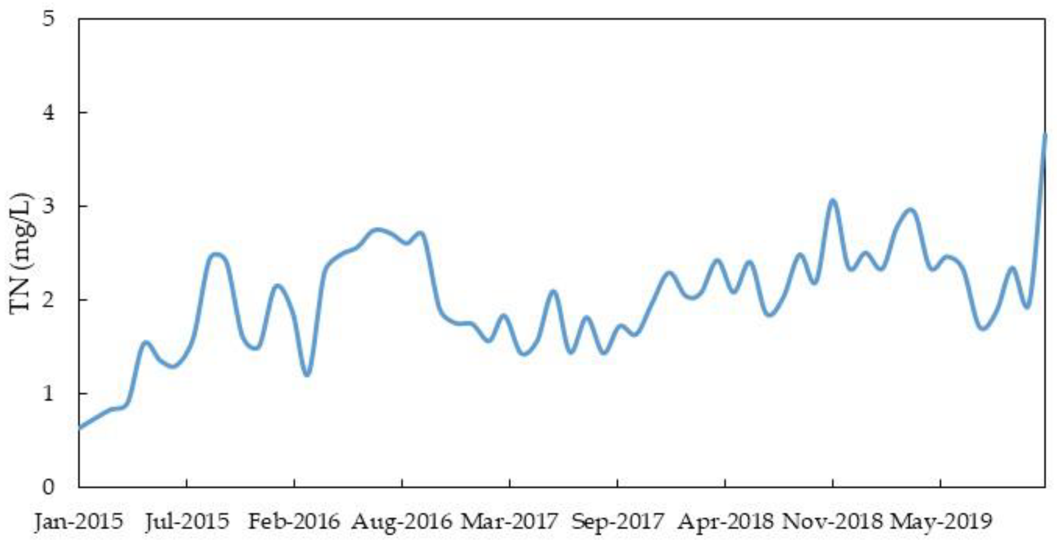
Compared with the monitoring data, the relative errors (Res) in the TN and TP loads were −45.36% and 18.09%, respectively. Based on the Second National Pollution Source Survey, the agricultural NPS of Gaofeng, Hongfenghu, Huchao, and Machang were estimated. The TN and TP loads in 2017 were increased by 59.57% and 7.71% more than the baseline year (2013), respectively (

Table 4. TN and TP loads in four towns in 2013 and 2017.

Year	TN (t)	TP (t)
2013	427.51	55.27
2017	682.19	59.53
Trend	+59.57%	+7.71%

). The water quality monitoring data (Figure 10 and Figure 11) revealed average increases of 30.76% and 12% in TN and TP water concentrations, respectively, in 2017. The change trends of the simulated results were consistent with the water quality monitoring data, and the results are reasonable.

To further verify the reliability of the model simulation results, some typical results from the literature on the NPS pollution path-through rate of China were reviewed (

Table 5. Results of the other studies on the path-through rate of NPS pollution in China.

Study Area	Scale	Model	λTN	λTP	Reference
Hongfenghu reservoir watershed	Mesoscale	PTRE-NPS	0.03−0.36	0.03−0.42	This study
Laodaohe watershed	Mesoscale	NANI	0.042−0.155	−	[39]
Haihe Basin	Large scale	ECM	0.109−0.904	0.084−0.317	[40]
Xinanjiang River Basin	Large scale	Investigation and monitoring	0.20	0.21	[41]
Downstream plain polder area of Ganjiang	Middle scale	Investigation	0.141−0.143 (Rural population)	0.129−0.137 (Rural population)	[42]
Laizhou Bay	Large scale	Pollutant load estimation method	0.1 (Farmland) 0.25 (Rural population) 0.07 (Livestock)	0.1 (Farmland) 0.25 (Rural population) 0.07 (Livestock)	[43]

). Based on the analyses mentioned as follows, the results of the PTRE-NPS of TN in this study are similar to those of other studies. The PTRE-NPS of TP is higher, which is probably because the study area is in the southwest of China, which is characterized by karst landform. Moreover, phosphorus in agricultural NPS is transported by soil erosion in the particulate form, and in the southwest of China, abundant rainfall leads to more soil erosion compared with other research areas with scarce rainfall.

4. Conclusions

The main conclusions are summarized below:

• The constructed PTRE–NPS model was successfully applied in simulations of agricultural NPS in the Hongfenghu reservoir watershed, which occupies Guiyang and Anshun Cities in the Guizhou Province of China. The TN and TP loads into rivers and lakes were 1707.78 and 209.03 t, respectively, with Re values of −45.36% and 13.07%, respectively. The simulation accuracy of the PTRE-NPS was acceptable. Baiyun Town presented the highest PTRE–NPS for both TN and TP.
• Baiyun, Shizi, Yangchang, Chengguan, and Machang are the high-risk townships for pollution by agricultural nonpoint TN, collectively accounting for 56.73% of the TN load. Baiyun, Shizi, and Chengguan are also at high risk of TP pollution from agricultural nonpoint sources, collectively accounting for 45.15% of the TP load. The key pollution sources of TN and TP were cultivated land and livestock/poultry farming, respectively. Therefore, they should be considered for taking effective control measures to control nonpoint source pollution.
• Compared with other methods of estimating the path-through rate for NPS pollutants, such as field monitoring, and the ECM, the PTRE-NPS model can scientifically represent the generation–migration–transmission process of agricultural nonpoint source pollutions in each grid at both the watershed and administrative scales. The model can also be used as an effective tool to identify transport paths for NPS pollution.

This paper simulated the pollution source data over one year. In the future, supplementary field monitoring should be performed to decrease the uncertainty. After years of collecting the pollution source data, the long-term stability of the model will be verified.

References

- Fleming, P.; Stephenson, K.; Collick, A.; Easton, Z. Targeting for nonpoint source pollution reduction: A synthesis of lessons learned, remaining challenges, and emerging opportunities. J. Environ. Manag. 2022, 308, 114649. [Google Scholar] [CrossRef] [PubMed]
- Ministry of Ecology and Environment of the People’s Republic of China. Bulletin of the Second National Census of Pollution Sources of China; Ministry of Ecology and Environment of the People’s Republic of China: Beijing, China, 2020.
- Zhu, X.; Lu, J.X. Nonpoint source pollution and soil erosion Control—Application of the Universal Soil erosion Equation in the United States. Trends Environ. Sci. 1984, 11, 2–8. [Google Scholar]
- Li, H.E. Application of hydrological models to non-point source pollution studies. Shaanxi Water 1987, 3, 18–23. [Google Scholar]
- He, C.S.; Fu, B.J.; Chen, L.D. Non-point source pollution control and management. Environ. Sci. 1998, 88–92, 97. [Google Scholar]
- Xu, Q.G.; Liu, H.L.; Shen, Z.Y.; Xi, B.D. Characteristics on nitrogen and phosphorus losses in the typical small watershed of the Three Georges Reservoir area. Acta Sci. Circum. 2007, 27, 326–331. [Google Scholar]
- Wang, X.Y.; Zhang, Y.F.; Ou, Y.; Yan, Y.M. Predicting effectiveness of best management practices for control of nonpoint source pollution—a case of Taishitun Town, Miyun County, Beijing. Acta Sci. Circum. 2009, 29, 2440–2450. [Google Scholar]
- Shen, Z.Y.; Liao, Q.; Hong, Q.; Gong, Y. An overview of research on agricultural nonpoint source pollution modelling in China. Sep. Purif. Technol. 2012, 84, 104–111. [Google Scholar] [CrossRef]
- Yang, G.X.; Best, E.P. Spatial optimization of watershed management practices for nitrogen load reduction using a modeling-optimization framework. J. Environ. Manag. 2015, 161, 252–260. [Google Scholar] [CrossRef]
- Johnes, P. Evaluation and management of the impact of land use change on the nitrogen and phosphorus load delivered to surface waters: The export coefficient modelling approach. J. Hydrol. 1996, 183, 323–349. [Google Scholar] [CrossRef]
- Geng, R.Z.; Yin, P.H.; Zhou, L.L.; Wang, M. Review: Assessment and calculation for the pass through rate of agricultural diffuse sources pollution in national scale. Environ. Sustain. Dev. 2019, 44, 26–30. [Google Scholar]
- Cherry, K.; Shepherd, M.; Withers, P.; Mooney, S. Assessing the effectiveness of actions to mitigate nutrient loss from agriculture: A review of methods. Sci. Total Environ. 2008, 406, 123. [Google Scholar] [CrossRef] [PubMed]
- Buchanan, B.P.; Josephine, A.A.; Zachary, M.E. A phosphorus index that combines critical source areas and transport pathways using a travel time approach. J. Hydrol. 2013, 486, 123–135. [Google Scholar] [CrossRef]
- Li, W.; Liu, S.; Liu, H. Review on Phosphorus Indices as Risk—Assessment Tools at Home and Abroad. Chin. J. Soil Sci. 2016, 47, 489–498. [Google Scholar]
- Arnold, J.G.; Fohrer, N. SWAT2000: Current capabilities and research opportunities in applied watershed modelling. Hydrol. Process. 2005, 19, 563–572. [Google Scholar] [CrossRef]
- Chahor, Y.; Casalí, J.; Giménez, R. Evaluation of the AnnAGNPS model for predicting runoff and sediment yield in a small Mediterranean agricultural watershed in Navarre. Agric. Water Manag. 2014, 134, 24–37. [Google Scholar] [CrossRef]
- Mohamoud, Y.M.; Parmar, R.; Wolfe, K. Modeling Best Management Practices (BMPs) with HSPF; American Society of Civil Engineers (ASCE): Reston, FL, USA, 2010. [Google Scholar]
- Majhi, A.; Shaw, R.; Mallick, K.; Patel, P.P. Towards improved USLE-based soil erosion modelling in India: A review of prevalent pitfalls and implementation of exemplar methods. Earth-Sci. Rev. 2021, 221, 103786. [Google Scholar] [CrossRef]
- Wischmeier, W.H.; Smith, D.D. Predicting Rainfall Erosion Losses: A Guide to Conservation Planning; USDA Agricultural Handbook No. 537; Science and Education Administration, U.S. Department of Agriculture: Washington, DC, USA, 1978.
- Chen, T.; Niu, R.Q.; Li, P.X.; Zhang, L.P.; Du, B. Regional soil erosion risk mapping using RUSLE, GIS, and remote sensing: A case study in Miyun Watershed, North China. Environ. Earth Sci. 2011, 63, 533–541. [Google Scholar] [CrossRef]
- Ding, X.; Shen, Z.Y.; Hong, Q.; Yang, Z.; Wu, X.; Liu, R. Development and test of the export coefficient model in the upper reach of the Yangtze River. J. Hydrol. 2010, 383, 233–244. [Google Scholar] [CrossRef]
- Beven, K.; Kirkby, M.J. A physically based, variable contributing area model of basin hydrology. Hydrol. Sci. Bull. 1979, 24, 43–69. [Google Scholar] [CrossRef] [Green Version]
- Chen, Z.; Liu, X.; Zhu, B. Runoff estimation in hillslope cropland of purple soil based on SCS-CN model. Trans. Chin. Soc. Agric. Eng. 2014, 30, 72–81. [Google Scholar]
- He, Y.; Wang, X.; Duan, S. Characteristics of runoff and sediment during individual rainfall in upper area of Miyun Reservior. Trans. Chin. Soc. Agric. Eng. 2015, 31, 134–141. [Google Scholar]
- Coale, F.J.; Baugher, E.; Sims, J.T.; Leytem, A. Accelerated Deployment of an Agricultural Nutrient Management Tool in Response to Local Government Policy: The Maryland Phosphorus Site Index. J. Environ. Qual. 2002, 31, 1471–1476. [Google Scholar] [CrossRef] [PubMed]
- Ralf, K.; Christoph, H.; Christian, W. Quantification of nitrate leaching from German forest ecosystems by use of a process oriented biogeochemical model. Environ. Pollut. 2011, 159, 3204–3214. [Google Scholar]
- Endreny, T.A.; Wood, E.F. Watershed weighting of export coefficients to map critical phosphorous loading areas. J. Am. Water Resour. Assoc. 2003, 39, 165–181. [Google Scholar] [CrossRef]
- Sharpley, A.; Kleinman, P.; Baffaut, C.; Beegle, D.; Bolster, C.; Collick, A.; Easton, Z.; Lory, J.; Nelson, N.; Osmond, D. Evaluation of phosphorus site assessment tools: Lessons from the USA. J. Environ. Qual. 2017, 46, 1250–1256. [Google Scholar] [CrossRef] [Green Version]
- Sharpley, A.N.; Kleinman, P.J.; Flaten, D.N.; Buda, A.R. Critical source area management of agricultural phosphorus: Experiences, challenges and opportunities. Water Sci. Technol. 2011, 64, 945–952. [Google Scholar] [CrossRef]
- Panagopoulos, Y.; Makropoulos, C.; Mimikou, M. Diffuse surface water pollution: Driving factors for different geoclimatic regions. Water Resour. Manag. 2011, 25, 3635–3660. [Google Scholar] [CrossRef]
- Panagopoulos, Y.; Makropoulos, C.; Mimikou, M. Reducing surface water pollution through the assessment of the cost-effectiveness of BMPs at different spatial scales. J. Environ. Manag. 2011, 92, 2823–2835. [Google Scholar] [CrossRef]
- Biddau, R.; Cidu, R.; Da Pelo, S.; Carletti, A.; Ghiglieri, G.; Pittalis, D. Source and fate of nitrate in contaminated groundwater systems: Assessing spatial and temporal variations by hydrogeochemistry and multiple stable isotope tools. Sci. Total Environ. 2019, 647, 1121–1136. [Google Scholar] [CrossRef]
- Bu, H.M.; Song, X.F.; Zhang, Y.; Meng, W. Sources and fate of nitrate in the Haicheng River basin in Northeast China using stable isotopes of nitrate. Ecol. Eng. 2017, 98, 105–113. [Google Scholar] [CrossRef]
- Steenhuis, T.S.; Winchell, M.; Rossing, J. SCS runoff equation revised for variable-source runoff areas. J. Irrig. Drain. Eng. 1995, 121, 234–238. [Google Scholar] [CrossRef]
- Lyon, S.W.; Walter, M.T.; Gerard-Marchant, P. Using a topographic index to distribute variable source area runoff predicted with the SCS curve-number equation. Hydrol. Process. 2004, 18, 2757–2771. [Google Scholar] [CrossRef]
- Sharpley, A.N.; McDowell, R.W.; Weld, J.L. Assessing site vulnerability to phosphorus loss in an agricultural watershed. J. Environ. Qual. 2001, 30, 2026–2036. [Google Scholar] [CrossRef] [PubMed] [Green Version]
- Verma, R.K.; Verma, S.; Mishra, S.K.; Pandey, A. SCS-CN-Based Improved Models for Direct Surface Runoff Estimation from Large Rainfall Events. Water Resour. Manag. 2021, 35, 2149–2175. [Google Scholar] [CrossRef]
- Liu, J.; Pang, S.; He, Y.; Wang, X. Critical area identification of phosphorus loss based on runoff characteristics in small watershed. Trans. Chin. Soc. Agric. Eng. 2017, 33, 241–249. [Google Scholar] [CrossRef]
- Fan, X.; Wu, F.P.; Meng, C.; Ye, L.; Li, X.; Zhang, M.Y.; Li, Y.Y.; Wu, G.Y.; Wu, J.S. Estimation of nitrogen output load of a river watershed based on net anthropogenic nitrogen input and river inflow coefficient. J. Agric.-Environ. Sci. 2021, 40, 185–193. [Google Scholar]
- Xing, B.Q.; Chen, H. Estimation of agricultural non-point source pollution load and river inflow coefficient in Beijing. Soil Wat Con. Chin. 2016, 5, 34–37. [Google Scholar]
- Yang, D.H. Analysis on aquatic environment of Anhui Province in Xinanjiang River watershed. Water Resour. Prot. 2006, 5, 77–80. [Google Scholar]
- Su, B.L.; Yuan, J.Y.; Li, H.; Luo, Y.X.; Zhang, Q. Loss rates of rural domestic pollutants in the down-stream plain polder area of Ganjiang. J. Beijing Norm. Univ. (Nat. Sci.). 2013, 449, 256–260. [Google Scholar]
- Zhou, L.L.; Geng, R.Z. Development and assessment of a new framework for agricultural nonpoint source pollution control. Water 2021, 13, 3156. [Google Scholar] [CrossRef]
Figure 1.
Location of Hongfenghu reservoir watershed in the Guiyang and Anshun Cities of Guizhou Province, China.
Figure 2.
The framework of the PTRE-NPS model.
Figure 3.
Spatial distribution of major parameters of PTRE–NPS of TN in the Hongfenghu reservoir watershed.
Figure 4.
Spatial distribution of major parameters of PTRE–NPS of TP in the Hongfenghu reservoir watershed.
Figure 5.
Spatial distribution of PTRE–NPS of TN and TP in the Hongfenghu reservoir watershed.
Figure 6.
PTRE–NPS of TN at the town scale in the Hongfenghu reservoir watershed.
Figure 7.
PTRE–NPS of TP at the town scale in the Hongfenghu reservoir watershed.
Figure 8.
TN loads at the town scale in the Hongfenghu reservoir watershed.
Figure 9.
TP loads at the town scale in the Hongfenghu reservoir watershed.
Figure 10.
Annual TN concentrations in the Hongfenghu reservoir watershed from 2015 to 2019.
Figure 11.
Annual TP concentrations in the Hongfenghu reservoir watershed from 2015 to 2019.