
Parametric Vine Copula Framework in the Trivariate Probability Analysis of Compound Flooding Events


Department of Civil and Environmental Engineering, Western University, London, ON N6A 5B8, Canada
*
Author to whom correspondence should be addressed.
Water 2022, 14(14), 2214; https://doi.org/10.3390/w14142214
Submission received: 16 June 2022
/
Revised: 9 July 2022
/
Accepted: 11 July 2022
/
Published: 13 July 2022
(This article belongs to the Section Hydrology)
Abstract
:The interaction between oceanographic, meteorological, and hydrological factors can result in an extreme flooding scenario in the low-lying coastal area, called compound flooding (CF) events. For instance, rainfall and storm surge (or high river discharge) can be driven by the same meteorological forcing mechanisms, tropical or extra-tropical cyclones, resulting in a CF phenomenon. The trivariate distributional framework can significantly explain compound events’ statistical behaviour reducing the associated high-impact flood risk. Resolving heterogenous dependency of the multidimensional CF events by incorporating traditional 3D symmetric or fully nested Archimedean copula is quite complex. The main challenge is to preserve all lower-level dependencies. An approach based on decomposing the full multivariate density into simple local building blocks via conditional independence called vine or pair-copulas is a much more comprehensive way of approximating the trivariate flood dependence structure. In this study, a parametric vine copula of a drawable (D-vine) structure is introduced in the trivariate modelling of flooding events with 46 years of observations of the west coast of Canada. This trivariate framework searches dependency by combining the joint impact of annual maximum 24-h rainfall and the highest storm surge and river discharge observed within the time ±1 day of the highest rainfall event. The D-vine structures are constructed in three alternative ways by permutation of the conditioning variables. The most appropriate D-vine structure is selected using the fitness test statistics and estimating trivariate joint and conditional joint return periods. The investigation confirms that the D-vine copula can effectively define the compound phenomenon’s dependency. The failure probability (FP) method is also adopted in assessing the trivariate hydrologic risk. It is observed that hydrologic events defined in the trivariate case produce higher FP than in the bivariate (or univariate) case. It is also concluded that hydrologic risk increases (i) with an increase in the service design life of the hydraulic facilities and (ii) with a decrease in return periods.
1. Introduction
Low-lying coastal area flooding can be defined by multiple flood-driving sources, such as oceanographic (storm surge or storm tide), meteorological (rainfall as a proxy of the direct surface runoff, also called pluvial flooding), and hydrological (river discharge or fluvial flooding), which may be naturally intercorrelated [1]. These extreme or non-extreme events can occur either successively or in close succession, called compound flooding (CF) events, resulting in severe consequences [2,3]. For instance, common meteorological forcing mechanisms, tropical or extra-tropical cyclones (or low atmospheric pressure systems), drive the storm surge and rainfall (which might result in high river discharge), resulting in CF events. Several compound extreme phenomena have been recorded in the last decade worldwide, for instance, Hurricane Igor in Canada, Cyclone Nargis in Myanmar, Hurricane Katrina in the United Kingdom, or Hurricane Harvey in the United States, etc. [4,5,6,7]. Rapid urban sprawl and climate change can further exaggerate the severity, or risk level, of coastal extremes worldwide [8,9,10]. Rising sea levels cause changes in the magnitude and frequency of coastal flooding due to the combined effects of high spring tides, storm surge, extreme precipitation, surface waves and increased river discharge. One study [11] pointed out that storm surge can be the primary driver responsible for coastal flooding. On the other side, when storm surge mixes with other hydro-meteorological events such as rainfall (pluvial) or river discharge (fluvial), they may result in extreme hazards [3,12]. The potential compounded impact of the joint occurrence of different drivers of flooding is examined in the literature, for example, between rainfall and storm tides [13], storm surge and sea-level rise (SLR) [14], high river discharge and coastal water level (WL) [3], and rainfall and storm surge [12].
Despite improved flood protection and advancements in flood forecasting and warning, the coastal regions are still highly threatened by severe flooding. The validity of univariate probability analyses would be questionable. A compound event is a multidimensional phenomenon where the likelihood of the joint occurrence of multiple intercorrelated events will be higher than expected, considering each random vector independently. The traditional statistical approaches usually account for the number of extreme joint episodes between the proxy variables of different flood hazard types using the multivariate statistical frameworks [15,16,17]. Recently, the copula function has been recognised as a highly flexible multivariate tool widely accepted in modelling extreme hydrologic events [18,19,20,21]. The copula function can accommodate a broader range of dependency and allow the modelling of univariate marginal distribution and their joint dependence structure separately. In the recent literature, the copula function gained more attention in modelling compound events [2,3,22], but all such incorporations are often limited to the bivariate joint case. For instance, 2D parametric family copulas are frequently used in joint dependency modelling targeting several flood-driving factors, such as storm surge (or storm tide) and rainfall, or storm surge (or storm tide) and river discharge. The coastal region flooding events can exhibit complex mutual concurrency between multiple (more than two) interacting variables. In other words, they can be characterised more comprehensively by simultaneously including the multiple factors (storm surges, rainfall, river discharge) instead of visualizing the pairwise joint dependence structures. A trivariate (or higher dimensional) joint distribution is rarely used in hydrologic risk assessments associated with the compound events.
Limited examples in the literature report the use of different 3D copula frameworks in the trivariate analysis and also highlight its flexibility and limitations [23,24,25,26]. For instance, in the trivariate or any higher dimensional analysis, the applicability of traditional symmetric Archimedean copulas would be impractical in preserving all lower-level dependencies among multiple intercorrelated random pairs. The multidimensional CF event can exhibit complex heterogeneous dependencies among variables of interest (e.g., storm surge, rainfall, or river discharge). In this 3D copula framework, all the mutual concurrencies must be averaged to the same value where the selected copula utilises a single dependence parameter to approximate their joint dependence structure. This copula’s structure can be an appropriate choice when all the random pairs’ correlation structures are identical, but this assumption could be impractical. In addition, the performance of the meta-elliptical class known as Gaussian copula would be questionable and have limitations under low probabilities unless the asymptotic properties of data are justified through solid arguments. It could not capture extreme tail dependence behaviour at the upper-right or lower-left quadrant tail. To overcome this modelling issue, asymmetric or fully nested Archimedean (FNA) copulas could be a better choice due to the multiple parametric joint asymmetric functions involved [27,28,29]. The FNA models can capture different inter-dependencies between and within the other groups of extreme variables and provide better flexibility in building a higher dimensional structure.
The justifiable preservation of all the lower-level dependencies is often challenging in the higher dimensional copula simulations, especially when a complex pattern of dependencies is exhibited. The FNA copula framework is only practical when two correlation structures are near or equal and smaller than the third correlation structure [26] and only limited to the positive range. As the dimension increases, only a narrow range of negative dependencies are permissible in the asymmetric FNA framework [30]. To overcome all the above-raised statistical issues, the vine or pair-copula construction (PCC) can be a practical and highly flexible approach to modelling high dimension extreme events [31,32,33,34]. The vine copula framework can provide a more flexible dependence structure and comprehensive way of approximating joint structure by mixing multiple 2D (bivariate) copulas in a stage-wise hierarchical nesting procedure. Due to conditional mixing, the framework can facilitate flexible modelling environments by eliminating the restriction of assigning a fixed multivariate copula structure to all variables of interest. Recently, a number of studies incorporated vine copula in modelling flood characteristics [35,36], drought [37], and rainfall modelling [38]. The incorporation of the vine copula in the modelling of compound phenomena is rare worldwide, e.g., [39,40] and has never been used in Canada.
According to Public Safety Canada [41], flooding can be considered one of the costliest natural disasters in Canada, continuously hurting the economy and causing infrastructure failures, loss of life, and damage to the ecological systems. On the other side, climate change significantly increases the risk of extreme events [42], both Canada’s east and west coasts have been experiencing an SLR throughout this century [43]. According to the Environment Ministry of British Columbia [44], the sea level is expected to increase by about half a meter by the end of 2050 and one meter by 2100. A recent study by Pirani and Najafi [4] pointed out the increasing risk of compounded flooding over Canada’s Pacific (west) and Atlantic (east) coasts due to a combination of streamflow, precipitation and tidal water level extremes. Extreme water levels can further increase the risk of high storm surge; at the same time, when this is combined with rainfall and fluvial flooding (or high river discharge), the results can be devastating. On the other side, climate change impacts can affect the severity and frequency of extreme precipitation, storms of greater intensity, and rising sea levels leading to an increased likelihood of flood risks. Overall, it is concluded that the complex interplay between storm surge, rainfall, and river discharge can exacerbate the impact of flooding events in the coastal regions of Canada. Thus, the simultaneous consideration of the compounding effect of these triplet variables can improve our understanding of flood risk. To the best of the authors’ knowledge, the incorporation of higher dimensional probabilistic framework in the joint modelling of compound flooding (CF) extremes is not available for the Canadian estuarine or coastal areas. This study is a part of the research project that aims to develop a trivariate probabilistic framework for modelling the risk of flooding events in Canada’s coastal regions (west and east). Each methodological finding is documented in a separate manuscript [45]. This manuscript presents new work by introducing vine copula-based methodology.
The present study goal is addressed by: (1) the development of a trivariate probability distribution framework by incorporating the 3D vine copula framework and comparing its performance with 3D fully nested Archimedean (FNA) copula in compounding the joint occurrence of rainfall, storm surges, and river discharge observations; and (2) the estimation of the trivariate joint and conditional joint return periods and failure probability statistics using the best-fitted model in the assessments of hydrologic risk. The present work’s primary methodological significance is in constructing the n-dimensional vine copula. The previous work (Daneshkhan et al. [35] and Vernieuwe et al. [38]) used the strength of dependency between given random pairs as the guidance for selecting and locating the random variable to be used as a conditioning variable in the D-vine structure. For example, suppose the strongest dependencies are exhibited between random pairs (X, Y) and (Z, Y). In that case, variable Y must be placed between the other two variables in constructing the drawable or D-vine structure. In this paper, we present a much more practical approach to developing vine structure first, placing each random variable at a centre (conditioning variable) separately and then identifying the best 3D vine structure to develop the multivariate dependence structure. In addition, this paper explores the applicability of failure probability (FP) statistics to the trivariate hydrologic risk analysis of rainfall, storm surge, and river discharge, work which has never been done before to the best of the authors’ knowledge. In previous work, researchers [3] used FP statistics to assess bivariate coastal flood risk between fluvial flow and coastal water (also future sea-level rise). While others [22] also incorporated FP statistics to perform bivariate hydrologic risk between rainfall and river discharge events and reference therein. The following Section of the paper presents the methodological framework developed in this research. Section 3 of the paper describes the application of the developed 3D vine copula framework to a case study of Canada’s west coast to investigate the compound effect of rainfall, storm surge, and river discharge observations on flood risk. The research summary and conclusions are presented in Section 4. All the estimated trivariate joint and conditional joint return periods and FP statistics can be used in the water infrastructure design and management in the coastal areas.
2. Methodological Framework
2.1. Trivariate Joint Probability Analysis via a Fully Nested Copula Framework
The complex and heterogeneous dependency in the CF events can demand a highly flexible multivariate framework that can comprehensively approximate the flood dependence structure’s probability density, and corresponding measures are capable of practical flood hazard assessments. The present study investigates the modelling adequacy of 3D vine copula in the trivariate analysis of storm surge, rainfall and river discharge observations in assessing compounded flood risk on the west coast of Canada. The performance of the recommended vine copula is compared with some frequently used asymmetric (or FNA) versions of Archimedean copulas, such as Clayton, Frank, and Gumbel–Hougaard (G–H) (refer to Supplementary Table S1). In reality, flood attribute pairs define CF events that usually exhibit different dependency levels called heterogeneous. Incorporating multiple best-fitted bivariate copulas between each flood pair in a stage-wise hierarchical nesting approach can be more practical than assigning a fixed trivariate structure. Because each pair-copula can be parameterised differently, vine copula allows each flood pair to have different strengths and types of dependence. Therefore, statistically, it is revealed that the vine approach can effectively tackle the heterogeneous dependency and approximation of joint density of the CF events comprehensively. Figure 1 illustrates the methodological work steps followed in the study.
Saklar [46] introduces the copula function concept [47]. The bivariate (2D) (or multivariate) joint cumulative distribution functions (CDFs) (or of random observations () (or (with continuous univariate marginal distribution functions ((or ( can be expressed as:
where and are the two-dimension (2D) and n-dimension copula functions. is the copula dependence parameters. Furthermore, the bivariate (2D) Archimedean copula can be mathematically expressed as:
where and are the selected Archimedean copula’s generator function and their inverse.
The 3D vine copula framework development requires fitting multiple 2D copulas in the D-vine structure’s trees (Tree 1 and Tree 2) (refer to the following Section 2.2 for details and their statistical approach). Fifteen different 2D parametric copulas are tested as candidate functions in modelling the bivariate joint dependence structure; refer to Supplementary Table S2. The dependence parameters of the fitted 2D copulas are estimated using the maximum pseudo-likelihood (MPL) estimation procedure [48,49,50].
The MPL estimator used the rank-based empirical distribution approach without depending on the marginal distribution of the targeted random observation.
The FNA copula comprises two or more ordinary two-dimension or higher-dimensional Archimedean copulas by another Archimedean copula, also called parent Archimedean copula [26,28]. Mathematically, the 3D FNA structure can be expressed as:
where the first derivative of is completely monotonic where and are Laplace transforms, and symbol ‘’ represents the composite function. in Equation (4) are the inner and outer copula of the fitted 3D FNA copulas. The random pair ( has the bivariate marginal distribution in the form of Equation (1) with a Laplace transform . Similarly, other random pairs ( and have the bivariate margins in the form of Equation (1) with Laplace transform .
The copula simulation via an asymmetric framework is complex and not be rich enough to model higher dimensional extreme events, already discussed in Section 1. Besides this, Venter et al.’s [51] study already pointed out that it is challenging to approximate most multivariate copula joint densities with an increase in their dimension.
2.2. A 3D Vine Copula Framework for the Trivariate Analysis
The vine copula originates from the works by Joe [30], and the underlying structural theory was extended by Bedford and Cooke [31]. The critical idea of vine copula-based methodology is to decompose the joint density function into a cascade of the local building blocks of the bivariate (2D) copula functions and their conditional and unconditional distribution functions [32,33,52,53]. In other words, a vine copula mixes (conditional) bivariate copulas in a stagewise hierarchical nesting procedure to build a high-dimensional (n-dimensional) multivariate joint density structure.
Under a regular vine framework, the distinct varieties of vine copula decomposition are canonical or C-vine and drawable or D-vine distribution. They represent the two modes of parametric regular vine construction [53,54]. The previous study observed that the D-vine copula’s applicability is widespread because of its higher flexibility than the C-vine structure [34,35]. The applicability of the D-vine structure seems more effective if we want to consider all mutual intercorrelations between the targeted random variables one after the other. Nevertheless, there is no difference between C- and D-vine frameworks when considering a 3D (or trivariate) joint distribution framework [36,52]. The construction of an n-dimensional vine copula framework can demand 2D (bivariate) copulas and have tree levels. Figure 2 illustrates the general structure of constructing a three-dimensional D-vine copula joint analysis.
Mathematically, the D-vine copula in the 3D joint distribution modelling can be expressed as:
where
where and are the conditional cumulative densities that can be estimated using the pair-copula densities.
The present study targeted three flood contributing variables (, rainfall, storm surge, and river discharge, in building a 3D vine copula framework to model CF events. The present 3D vine simulation can comprise two trees (Tree 1 and Tree 2), five nodes, and three edges (Figure 2). This D-vine copula simulation can require three best-fitted 2D parametric copulas to model the trivariate dependence structure via stage-wise hierarchical nesting. Referring to Figure 2, the first tree (Tree 1) comprises two best-fitted 2D copulas, say and , in capturing the joint dependence structure between each random pair (between flood pairs rainfall (R)–storm surges (SS) and also storm surges (SS) –river discharge (RD)). The graphical illustration in Figure 2 considered river discharge (RD) as a conditioning variable (positioning at the centre of the D-vine structure). The selected best-fitted 2D copulas in Tree 1 are employed further in deriving the conditional cumulative distribution functions (CCDFs), also called the h-function. CCDFs are estimated by taking the partial derivative of the best-fitted 2D copula with respect to the conditioning variable and can be evaluated by:
Also, the generalised form of Equation (7), for any trivariate random observations (say X, Z, Y), where variable Z is assumed conditioning variable, can be expressed as:
The estimated CCDFs obtained from Tree 1 (using Equation (7)) become the input in defining the best-fitted 2D copula , in the second tree (Tree 2). Finally, the full density structure of the 3D copula is estimated by
Also, the generalised form of Equation (9), in building full density trivariate structure for the variable sequences (say, X-Z-Y) (where variable Z is assumed conditioning variable, can be expressed as:
In this study, D-vine copula structures are developed in three alternative ways or cases, each by permutation of the conditioning variables, refer to Figure 3a–c. In the existing approach to constructing a vine copula framework, the conditioning variable, centred at the middle location of the D-vine structure, must be selected based on the strength of dependencies between the variables of interest. In the presented work, we offer a more practical solution of separately considering each variable as a conditioning variable in generating multiple vine structures and then determining the best-fitted D-vine structure that depends on the estimated fitness test statistics. This approach provides a better way of constructing a vine structure. In the first case of developing vine structure, Case 1, the D-vine framework is constructed by placing the river discharge (RD) observations (variable 3) in the centre, also called the conditioning variable (refer to Figure 3a). The storm surge (variable 2) and rainfall (variable 1) are conditioning variables in the second (Case 2) and third (Case 3) of constructing D-vine copula structures (refer to Figure 3b,c). The D-vine frameworks are built for three cases using Equations (5)–(8). The best-fitted D-vine structure is selected based on the goodness-of-fit (GOF) test statistics. Finally, the performance of the selected best-fitted D-vine structure is compared with the fitted 3D asymmetric or FNA copulas (refer to Supplementary Table S1) in defining the trivariate dependence structure of compound events.
2.3. Generating Random Observations from the Selected D-Vine Copula Structure
The present study is based on a random triplet of flood observations to model 3D CF events. In the vine copula analysis, the theory of the conditional mixture copula approach is employed to simulate random samples of any size or length, as already pointed in the literature [33,34,38,55]. The general algorithm for sampling n dependent uniform, [0, 1] variables is identical for the D- or C-vine copula structure. Let us consider a three-dimensional case to generate a random triplet observation out of the 3D conditional mixture copula (or 3D vine structure), with conditioning variables uniformly distributed in [0, 1]. A random sample which are uniformly distributed on [0, 1] should be generated first from . The following steps are used in the implementation process:
- Step 1: Estimating the first random variable,
- Step 2: Estimating the second random variable, , where
- Step 3: Estimating the third random variable, , where
- Step 4: Finally, the corresponding value of the flood characteristics (rainfall (R), storm surge (SS), and river discharges (RD)) are estimated by taking the inverse of the univariate marginal cumulative distribution function, Simulated rainfall (R) observations; Simulated storm surge (SS) observation; Simulated river discharge (RD) observations.
2.4. Probabilistic Analysis of Compound Flooding Events
2.4.1. Joint and Conditional Return Periods
Estimating the flood exceedance probability or design quantiles under different notation of return periods, for instance, joint return periods (JRPs) and conditional return periods, is essential in evaluating hydrologic risk. The present manuscript focused on two different return approaches based on the joint probability distribution relationship: OR- and AND-joint return periods (JRPs) [26,50,56,57]. For the trivariate joint distribution event (, the OR-joint RP is estimated using the best-fitted 3D copula, as given below.
where is the trivariate joint cumulative distribution functions (JCDFs) that can be expressed using the best-fitted D-vine copula along with best-fitted univariate flood marginals
In the second joint dependency situation, for instance, for a trivariate joint distribution event (, the AND-joint RP is estimated using the best-fitted 3D vine copula structure, as given below.
where are the bivariate JCDFs derived from the best-fitted 2D copula function.
In most engineering-based hydraulic or flood defence infrastructure designs, it would be demanding to consider a flood events situation by focusing on the importance of one flood variable over other variables via the conditional joint probability distribution relationship. To achieve this, the conditional return period of one variable given various percentile values of another variable is also examined in this study [19,26,58,59,60,61]. The present study estimates two different approaches to estimating conditional return periods (RPs):
Approach 1
For trivariate distribution case (via 3D vine copula):
The conditional return period of one flood variable (say, X = rainfall) conditioning to two other variables (say, = river discharge), is estimated by:
For bivariate distribution case (via 2D copula):
Approach 2
For trivariate distribution case (via 3D vine copula):
The conditional joint return period of two flood variables (say, X and Y) given various percentile values of the third flood variable can be estimated by:
Similarly, for bivariate distribution analysis via 2D copula:
2.4.2. Hydrologic Risk Evaluation of Flood Events
The estimated joint return periods (refer to Section 2.4.1) would be incapable of highlighting potential flood risk hazards during the entire project lifetime [22,62,63]. The estimated RPs would not account for the planning horizon [64]. In the hydrologic risk assessments, the importance of the risk of failure associated with the return period, called failure probability (FP), is already highlighted, as by Yen [65], Salvadori et al. [66], Serinaldi [67], and Moftakhari et al. [3], Xu et al. [68], and references therein. The FP statistics facilitate an effective and practical approach to hydrologic risk assessments rather than just considering the definition of return period values (joint RP). The incorporation of the FP statistics is limited to bivariate joint distribution cases [3,22,68]. The present study estimated FP statistics in examining the hydrologic risk associated with trivariate compound events, results are also compared with bivariate events.
Let us suppose, are the targeted triplet hydrologic series (where R, SS, and RD are abbreviations of rainfall, storm surges, and river discharge series, respectively) with an arbitrary project lifetime is T. The FP statistics can be mathematically expressed as
The risk of failure associated with return periods for the trivariate flood hazard scenario is estimated for the OR- joint case as given below:
3. Application
3.1. Study Area and Delineation of Compound Flooding Characteristics
This study introduces the vine copula framework in the trivariate analysis to assess the risk of CF events through compounding the joint impact of storm surge, rainfall, and river discharge with 46 years of observations of the west coast of Canada. The west coast parts of Vancouver, within low-lying regions near the Pacific Ocean and Fraser River, are highly vulnerable to coastal and river flooding. The area often experiences mature and large extra-tropical storm systems that often stall when encountering the coast mountains, creating the potential for prolonged impact. The Fraser River is located south of the Metro Vancouver, BC. It is the longest river in this province. Its annual discharge at its mouth is about 3550 m3/s, flowing for 1375 km and finally draining into the Strait of Georgia. This study is investigating the compound impact of storm surge, rainfall and river discharge events on flood risk in the coastal region. To achieve this task, the present work search for the annual maximum 24-h rainfall events and takes the highest storm surge and river discharge within a time range of ±1 days.
At first, the observed coastal water levels (CWL) are collected at the New Westminster tidal gauge station (tidal gauge station id 7654, ) and obtained from the Fisheries and Oceans Canada from 1970 to 2018. The CWL data are collected at chart datum (CD), and the geolocation is the Fraser River. On the other side, the Canadian Hydrographic Service (CHS) provides predicted astronomical high tide data. The storm surge values are then calculated by subtracting the high tide value from the CWL data for each calendar year. Estimating storm surges requires proper time matching between predicted high tides and CWL data.
The rainfall data is collected at the Haney UBC RF Admin gauge station (geographical coordinates ) for the same calendar year, where the selection of rain gauge station is solely based on proximity within a radial distance of 50 km from the targeted tidal gauge station. In other words, the nearest rainfall gauge station is assigned within a specified radial distance for the same time frame. The streamflow gauge station is also selected using the same approach. The daily streamflow discharge observations are collected at the gauge station Fraser River at Hope (geographical coordinates Lat and Long) and provided by the Environment and Climate Change Canada.
First, the annual maximum 24-h rainfall series are defined using daily-basis 24-h rainfall observations. After transforming the rainfall data into block (annual) maxima, the river discharge and storm surge values are identified within a time lag of day from when the rainfall attained their maximum values. It should be noted that because of several missing data for streamflow discharge observations between the years 1970 to 2018 when searched within a ±1 day of annual maximum 24-h rainfall, the present analysis only considered the 46 years of observations. The descriptive statistics of the extracted triplet flood characteristics are provided in the Supplementary Table S3. Supplementary Figure S1a–c illustrates some univariate plots, including histogram plot, box plot and normal Q-Q (quantiles-quantiles) plot of extracted flood characteristics, annual maximum 24-h rainfall (R), maximum storm surge (Time interval = day) (SS) and maximum river discharge (time interval = day) (RD).
3.2. Marginal Behaviour of the Targeted Flood Characteristics
Firstly, the Ljung and Box [69] test, based on a form of hypothesis testing called Q-statistics, is used to test the presence of serial correlation [35] (refer to Supplementary Table S4 and Supplementary Figure S2). It is found that all three flood variables exhibited zero autocorrelation. Similarly, time-varying consequences within individual flood series are examined using the nonparametric Mann–Kendall (M–K) test [70,71] and a modified M–K test [72] (refer to Supplementary Table S5). On the other side, the test for homogeneity is performed to examine if there is a time when a change occurs within individual flood characteristics. For this, four different tests are used such as Pettitt’s test [73], SNHT (Standard Normal Homogeneity Test) [74], Buishand’s test [75], and von Neumann’s ratio test [76]. The results of homogeneity tests are presented in Supplementary Table S6. Based on the results (refer to Tables S5 and S6), it is observed that both rainfall and river discharge observations exhibit time-invariant behaviour and have homogenous behaviour. But the storm surge exhibits time-varying behaviour and is non-homogenous at the significance level of 0.05 (refer to Tables S5 and S6). Supplementary Figure S3 shows the selected flood variables’ time series plot, indicating non-homogenous behaviour within storm surge observations. Therefore, pre-whitening is required to remove the time-trend or detrend the storm surge observations (see Supplementary Figure S4) and then use them in the univariate and multivariate modelling along with other selected flood variables, rainfall and river discharge.
Frequently used 1-D parametric distributions are tested in modelling univariate flood margins (refer to Supplementary Table S7). The parameters of the fitted distributions are estimated using the maximum likelihood estimation (MLE) procedure. The performance of the best-fitted univariate functions is tested using the Kolmogorov–Smirnov (K–S) test statistics [68], Anderson–Darling (A–D) test [77], and Cramer–Von Mises (C–VM) criterion [78,79] (refer to Supplementary Table S8). It is concluded that GEV, normal and GEV distribution are identified as the best fitted for defining the marginal distribution of annual maximum 24-h rainfall, maximum storm surge (Time interval = day) and maximum river discharge ( day) series (selected distributions have a minimum value of K–S test, A–D test and C–VM test statistics). The graphical visual inspection is also carried out using the probability density function (PDF) plot, cumulative distribution functions (CDF) plot, probability–probability (P–P) plot and quantile–quantile (Q–Q) (refer to Supplementary Figure S5a–c). It is concluded that the selected 1D probability function for each flood variable via an analytical approach supports the qualitative visual inspection.
3.3. Incorporating Vine Copula in the Trivariate Flood Dependence Structure
3.3.1. Approximating Bivariate Joint Dependence Structure via 2D Copulas
Both the parametric, Pearson’s linear correlation (r), and nonparametric rank-based correlation measures, Kendall’s tau (𝜏) and Spearman’s rho (ρ) correlation coefficient [48], are used to measure the degree of mutual concurrency. Table 1 presented the estimated correlation measured at a significance level of 0.05. A positive correlation is exhibited between the variable of interest. Besides the analytical approach, the graphical-based visual inspection is performed using the 3D scatterplot (Supplementary Figure S6), 2D chi-plot [80] (Supplementary Figure S7a–c), and 2D Kendall’s (K)-plot [81] (referred to Supplementary Figure S8a–c).
In this study, fifteen different parametric class 2D copulas (monoparametric, mixed and rotated versions of Archimedean copulas) are tested [47,82,83,84], refer to Supplementary Table S9a–c. The selected 2D copulas define the bivariate dependence structure of flood pairs, rainfall–storm surge, storm surge–river discharge, and rainfall–river discharge. The copulas dependence parameters are estimated using maximum pseudo-likelihood (MPL) estimators. The estimated 2D copulas dependence parameters are listed in Supplementary Table S9a–c.
The adequacy of the best-fitted 2D copulas fitted to each flood pair is tested using the Cramer–Von Mises (C–VM) functional test statistics, with parametric bootstrap sampling procedure with bootstrap sample N = 1000 [85,86], refer to Table S9a–c (minimum the value of test statistics must indicate a better fit, also their associated p-values must be greater than 0.05). Investigation reveals that BB7 copula is selected as the best-fitted for flood pair (rainfall–storm surge), Gumbel–Hougaard (G–H) for flood pair (storm surge–river discharge) and Survival BB7 for flood pair (rainfall–river discharge). To cross-validate the performance of the selected 2D copulas in capturing extreme behaviour, the tail dependence assessments are performed [87] (refer to Supplementary Table S10). In this regard, the value of the upper tail dependence coefficient (UTDC) is estimated via the nonparametric (, estimator suggested by Caperaa et al. [88]) and parametric estimates , and then compared (refer to Table S10). The minimum difference is observed between the nonparametric coefficient of UTDC and parametric coefficient of UTDC Overall, it is revealed that the selected 2D copulas satisfactorily capture extreme tail dependence behaviour. Supplementary Figures S9 and S10a–c illustrate the scatter plots, chi-plots, and K-plots drawn from the random samples (N = 1000) generated using the best-fitted 2D copulas fitted to flood pairs. Visual inspection supports the choice of analytically selected copulas. The selected 2D copulas are utilised to fit the 3D vine copula framework of Section 3.3.2. They are also used in estimating the bivariate joint and conditional joint return periods (RPs) in Section 3.4.1. Supplementary Figures S11a–d, S12a–d and S13a–d illustrate the joint probability density functions (JPDFs) and the joint cumulative distribution functions (JCDFs) plots derived from the best-fitted 2D copulas.
3.3.2. Constructing the D-Vine Copula Structure in the Trivariate Analysis
Three different D-vine structures are considered by permutation of conditioning variables in the first Tree (Tree 1), refer to Figure 3a–c in Section 2.2. The computation involved in developing three-dimensional D-vine copulas is performed using R software (R Core Team [89]) packages called Vine Copula [90] and Vines [91]. The construction of each D-vine structure is separately presented below:
1. Case 1 (D-vine structure 1): Placing maximum river discharge (Time interval = ±1 day) series (variable 3) as a centre or conditioning variable (referring to Figure 3a and Table 2 and Supplementary Table S11).
In the first tree (Tree 1), Survival BB7 () and Gumbel–Hougaard () copulas are selected (refer to Table S9b,c). The conditional cumulative distribution functions (CCDFs) (or h-function), and are estimated using Equation (7) or Equation (8). To identify the 2D copula in the second tree (Tree 2), where the input variables are and Clayton copula is selected as the best-fitted 2D structure , referring to Supplementary Table S11). Finally, the full density trivariate copula structure is obtained using Equation (9) (or Equation (10), assuming variable X = rainfall, Y = river discharge, Z= storm surge).
2. Case 2 (D-vine structure 2): Placing maximum storm surge (Time interval = ±1 day) series (variable 2) as a centre or conditioning variable (referring to Figure 3b and Table 2 and Supplementary Table S12).
In the first tree (Tree 1), BB7 () and Gumbel–Hougaard () copulas are selected between rainfall–storm surge and storm surge–river discharge (refer to Table S9a,b). The CCDFs ( and ) are estimated using Equation (8). Rotated BB8 270 degrees copula is selected as most parsimonious in the second tree (Tree 2), referring to Supplementary Table S12. Finally, the full density 3D structure is obtained using Equation (10) (assuming variable, X = rainfall, Y = storm surge, Z = river discharge).
3. Case 3 (D-vine structure 3): Placing rainfall series as a centre or conditioning variable (referring to Figure 3c and Table 2 and Supplementary Table S13).
Refer to Table S8a,c, BB7 and Survival BB7 copula is selected for the first tree (Tree 1) between flood pairs storm surge–rainfall and rainfall–river discharge. The estimated h-functions and is used in determining the best-fitted copula in the second tree (Tree 2). The Frank copula is identified as the best-fitted structure in Tree 2, (refer to Supplementary Table S13). The full density 3D vine-based joint density is obtained by using Equation (10) (assuming variable X = storm surge, Y = rainfall, Z = river discharge).
The performance of the above constructed D-vine structures is compared using information criterion statistics called Akaike information criterion (AIC) [92] and Bayesian information criterion (BIC) [93]. It is concluded that vine copula constructed by placing river discharge series as a conditioning variable, D-vine structure 1 (Case 1) exhibits a minimum value of both AIC and BIC test statistics (refer to Table 2). It also has the highest value of log-likelihood (LL) of the model compared to other vine structures (D-vine structures 2 and 3). Based on the above outcomes, it is inferred that this approach to constructing the vine copula framework is more practical by permuting the conditioning variable instead of fixing its location. For example, as we switched from Case 1 to Case 2, the D-vine copula structure’s performance was reduced by placing storm surge as a conditioning variable (refer to Table 2). It is also observed that model adequacy of D-vine structure 3 (Case 3) is much better than Case 2.
The adequacy of the above selected D-vine structures is compared with asymmetric FNA copulas, such as Frank, Gumbel, and Clayton (refer to Table S1). The dependence parameter of the fitted FNA copulas, both inner and outer copula, is estimated using the maximum likelihood estimation procedure, using the R library, HAC [94] (refer to Table 3 and Equation (4)). It is observed that the performance of the asymmetric Gumbel copula (the minimum value of AIC, BIC and highest value of LL) is best among the fitted 3D FNA copulas. Similarly, from Table 3, it is inferred that the performance of the selected D-vine copula structure 1 (Case 1) outperforms the best-fitted asymmetric Gumbel copula in the trivariate modelling of the compound flooding variables or events. The reliability and suitability of the selected D-vine copula are examined by comparing Kendall’s tau correlation coefficient calculated from the generated random samples (sample size N = 1000) using the best-fitted vine copula (D-vine structure 1) and asymmetric FNA copulas (Gumbel–Hougaard copula) and compared with the empirical Kendall’s coefficient estimated from the historical flood characteristics (refer to Table 4). The best-fitted D-vine structure 1 (Case 1) shows a minimum difference between the theoretical and empirical Kendall’s . It regenerates the correlation structure of historical flood variables more effectively.
Besides this, the performance of the selected D-vine structure is examined graphically using the overlapped scatterplot (refer to Supplementary Figure S14a) between the generated random samples (sample size N = 1000) derived from the fitted model. The random samples from the selected D-vine copula are estimated based on the algorithm presented in Section 2.3. It is concluded that the selected D-vine copula (Case 1) performs adequately since the generated random observations (indicated by light blue colour) overlapped with the natural mutual concurrency of the historical samples (red colour); refer to Supplementary Figure S14a. Supplementary Figure S14b illustrates a 3D scatterplot derived from the selected D-vine copula structure of sample size (N = 1000). In conclusion, the D-vine copula structure for Case 1 (centring river discharge as conditioning variable) provides a much more efficient approach in the trivariate joint modelling. It is thus further used in deriving the trivariate joint and conditional joint return periods (RPs). The estimated joint CDF derived from the fitted D-vine structure is employed further to estimate failure probability (FP), which is often considered a practical approach for assessing the hydrologic risk associated with CF events. Supplementary Figure S15a–c illustrate the joint density of 2D copulas families employed in constructing the selected D-vine copula structure (vine structure 1) in trivariate joint dependency modelling. The vine tree plot and matrix of the contour plot associated with the best-fitted D-vine structure is presented in Figure 4 and Supplementary Figure S16.
3.4. Assessing the Hydrologic Risk of Compound Flooding Events
3.4.1. Primary OR and AND Joint Return Period
The objective of frequency analysis is to establish an interlinking between design quantiles and their frequency of occurrence (or non-exceedance probability). The best-fitted D-vine structure 1 (refer to Table 2) is employed in estimating trivariate joint return periods for OR-joint and AND-joint cases, followed by Equations (11) and (12). Besides this, the bivariate OR- and AND-joint RPs, for flood pair, such as rainfall–storm surges, storm surges–river discharge, and rainfall–river discharge, are also estimated using the best-fitted 2D copulas (refer to Table S9a–c), followed by Brunner et al. [61] and Latif and Mustafa [95]. The comparative table of trivariate, bivariate, and univariate RPs are listed in Table 5. The investigation results pointed out that the value of AND-joint RP for any trivariate (and bivariate) flood events is higher than the OR-joint RP, . Hence it also concluded that the occurrence of trivariate flood characteristics simultaneously is less frequent in the “AND” case and more frequent in the “OR” joint case. For instance, consider 100 year flood events having the following characteristic (refer to Table 5), rainfall = 183.68 mm, storm surges = 0.401 m, river discharge = 10005.067 m3/s, the bivariate OR- and AND-joint RP is (between flood pair rainfall–storm surges), (between flood pair rainfall–river discharge), and (between flood pair storm surges–river discharge). Similarly, for a 100 year flood event with above mentioned flood characteristics (refer to Table 5), the trivariate OR- and AND-joint RPs is . From the above explanation, it could be more practical to account for both OR- and AND cases of trivariate joint return periods. It must be observed from the estimated values, refer to Table 5, how much it could be effective when simultaneously integrating the joint distribution behaviour of the above flood variable instead of just considering pairwise dependency modelling. Accounting for either AND- or OR-joint cases would be problematic in the flood risk analysis; in other words, their importance will solely depend on the nature of the problem. Otherwise, it might underestimate or overestimate the hydrologic risk associated with compound flooding (CF) events.
3.4.2. Conditional Joint Return Periods of CF Events
The conditional RP relies on the conditional probability distribution between the targeted flood contributing variable, given that some condition is fulfilled. Using Equations (13)–(16), the conditional RPs are estimated for trivariate (and bivariate) joint distribution cases (refer to Supplementary Figure S17a–f). It is observed that return period of trivariate flood decrease with an increase in the percentile value of the conditional flood variable, river discharge. For instance, flood events with the following characteristics, rainfall = 145.8 mm, storm surge = 0.68 m, the conditional joint RP is 47.20 years (when river discharge ≤ 1085 m3/s (25th percentile)), 41.86 years (when river discharge ≤ 1615 m3/s (50th percentile)), 35.25 years (when river discharge ≤ 2162.5 m3/s (75th percentile)), and 29.65 years (when river discharge ≤ 3100 m3/s (90th percentile)), and so on.
On the other side, the conditional joint return period of rainfall given various percentile values of storm surge and river discharge are illustrated in Figure 5 (using Equation (13)). It is observed that higher return periods are obtained from the lower percentile value of storm surge and river discharge observations than the lower river discharge and storm surge values for the same specified values of rainfall characteristics. For instance, in a flood event with flood characteristics, rainfall = 145.8 mm, the conditional JRP is 49.65 years (when storm surge ≤ 0.068 m and river discharge ≤ 1085 m3/s (25th percentile for both variables)), 43.25 years (when storm surge ≤ 0.23 m and river discharge ≤ 1615 m3/s (50th percentile for both variables)), and 29.97 years (when storm surge ≤ 0.45 m and river discharge ≤ 3100 m3/s (90th percentile for both variables)), and so on. Therefore, it is observed that the return period decreases with an increase in the percentile values of both conditional variables (storm surge and river discharge).
The conditional return periods of rainfall at given storm surge and constant river discharge, and conditional return period of rainfall at given river discharge and constant storm surge are presented in Figure 6 and Figure 7. Both storm surge and river discharge values correspond to various percentile of the respective data. It is observed that, by fixing the river discharge value, river discharge = 5377 m3/s (99th percentile value), the return period decreases with an increase in the percentile value of the storm surges. For instance, in a flood event with flood characteristics, rainfall = 145.8 m and river discharge = 5377 m3/s (constant), the return period is 40.70 years (when storm surge ≤ 0.06 m), 32.57 years (when storm surge ≤ 0.23 m), and 30.71 years (when storm surge ≤ 0.35 m). In conclusion, the RPs are higher at the lower value of storm surge than the lower storm surge for the same specified values of rainfall events. Also, from Figure 7, the estimated RP is lower at a higher conditional river discharge with a constant storm surge (storm surge = 0.62 m, 99th percentile value) than the lower river discharge for the same specified values of rainfall events. For instance, in a flood event with flood characteristics, rainfall = 145.8 m and storm surge = 0.62 m (constant, 99th percentile value), the return period are 47.26 years (when river discharge ≤ 1085 m3/s), 41.94 years (when river discharge ≤ 1615 m3/s), and 35.32 years (when river discharge ≤ 2162.5 m3/s), and so on.
Similarly, conditional return periods for the bivariate joint cases are also examined, return periods of rainfall conditioned to river discharge (or vice-versa) and rainfall conditioned to storm surge (refer to Supplementary Figures S18a–d and S19a–d). Figure S18a,b show that the conditional return periods of the storm surge events decrease with an increase in the percentile value of rainfall observation in both cases of the estimated conditional RPs, using Equations (14) and (16). Similarly, the conditional RPs of rainfall decrease with an increase in the value of storm surge (refer to Figure S18c,d). Comparing Figure S18a,c, it is concluded that higher return periods are obtained when conditioning to rainfall series than when considering storm surge as a conditioning variable.
The joint return period of rainfall events conditioned to river discharge observation (and vice-versa) is estimated using Equations (14) and (16), and their values are visually inspected in Supplementary Figure S19a–d. It is observed that the conditional return period of rainfall events (or river discharge) decreases with an increase in the river discharge (or rainfall) events. Also, by comparing Figure S19b,d, the conditional return period is higher when conditioned to the rainfall observation for different percentile values than when considering river discharge events as a conditioning variable.
3.4.3. Analysing the Hydrologic Risk of Flooding Events
FP statistics can define the probability of the potential flood events occurring at least once in a given project design lifetime. Figure 8a–e illustrates the variation in trivariate (bivariate and univariate) flood hazard scenarios by the service design lifetime under different return periods (RPs) of 100 years, 50 years, 20 years, 10 years, and 5 years. It is observed that trivariate flood events produce a higher failure probability (FP) than the bivariate (or univariate) flood events for OR-joint cases (refer to Figure 8a–e). For instance, at the return period RP = 100 years, the estimated value of FP for the trivariate (and bivariate) hazard scenario is 0.90 (and 0.84). However, when the return period RP is reduced to (RP = 50 years), the value of the trivariate (and bivariate) flood hazard scenario or FP is 0.85 (and 0.63). The trivariate (also bivariate) hydrologic risk decreases with an increase in the return period. At the same time, hydrologic risk value would increase with an increase in the service design lifetime of the hydraulic infrastructure. This point further inferred that the return period (RP) is not explicitly tied to a planning period and is ineffective in characterizing the chance of events occurring during a project lifetime. It is also concluded that ignoring trivariate probability analysis by compounding the joint impact of the targeted flood characteristics results in underestimating the failure probabilities FPs.
Similarly, the failure probability (FP) for a bivariate flood hazard scenario is estimated using Equation (17) for the bivariate OR-joint cases. For instance, the bivariate hydrologic risk for flood pair rainfall–storm surges and rainfall–river discharge is estimated. The variation of bivariate flood hazard scenarios (or FP statistics) for different design lifetimes of the hydraulic infrastructure is illustrated in Supplementary Figures S20a–g and S21a–g. The bivariate hydrologic risk for both flood hazard scenarios, rainfall–storm surge and rainfall–river discharge, increases with a decrease in return periods, and, at the same time, the value of FPs increases with an increase in the value of the design lifetime of the hydraulic infrastructure. It is also observed that bivariate events produce higher FP than univariate flood events.
Supplementary Figures S22a–c and S23a–c illustrate the variation of the bivariate hydrologic risk (or FP) with changes in the rainfall events in differently designed storm surges and river discharge events separately. The designed storm surge and river discharge series are considered for return periods, 200 years, 100 years, 50 years, 20 years, and 10 years. The project design lifetime (or service time of the hydraulic facilities) is assumed to be 100 years, 50 years, and 30 years. It is revealed that the bivariate hydrologic risk (joint analysis of flood pair rainfall–storm surge) increases with an increase in the project design lifetime (or service time) and decreases with an increase in the return period of storm surge observations. From the results shown in Figure S23a–c, the bivariate hydrologic risk (collective impact of rainfall and river discharge observations) increases with an increase in the project design lifetime (or service time). It decreases with an increase in the return period of river discharge observations.
In conclusion, the simultaneous accounting of the three flood characteristics considered, e.g., rainfall, storm surge, and river discharge, can enable us to better understand and visualise compound flooding and provide more critical information for flood risk assessments. These analytical and graphical investigations are vital for the sustainable design and planning of flood management strategies in coastal regions.
4. Research Summary and Conclusions
The complex interplay between storm surge, river discharge, and rainfall in the coastal region can exacerbate the impact of flooding, which cannot be neglected due to the common forcing mechanism responsible for driving these events. A comprehensive understanding of the probabilistic behaviour of CF events can be obtained by simultaneously considering these flood-contributing variables in a trivariate distribution framework. This paper introduces parametric vine copula-based methodology to the trivariate analysis of compound events by combing the joint probability of annual maximum 24-h rainfall series, storm surge, and river discharge observed within a time lag of ±1 day from the date of the highest annual 24-h rainfall event. The modelling adequacy of the developed vine copula framework is also compared with some asymmetric FNA (viz., Clayton, Gumbel–Hougaard and Frank) copula structures in accommodating trivariate flood dependency. The most parsimonious trivariate probability framework is selected and used to assess hydrologic risk in a case study on the west coast of Canada. The main findings of the present study are given below:
- No significant trend and serial correlation are identified within the time series of annual maximum 24-h rainfall and maximum river discharge (time interval = ±1 day). Moreover, both series exhibited homogenous behaviour. The maximum storm surge (time interval = ±1 day) showed a significant time trend and non-homogenous behaviour.
- The association among these mutually correlated flood variables is examined and used for dependency structure modelling of 3D copulas. The graphical and analytical investigation found that the dependence structure is statistically significant with positive dependency. Finally, the copula-based methodology is adopted for risk analysis of compound events.
- Firstly, BB7, Gumbel–Hougaard (G–H), and Survival BB7 copula are the most appropriate for describing dependence structures for flood pair rainfall–storm surge, storm surge–river discharge, and rainfall–river discharge, respectively. Besides this, upper tail dependence coefficient assessments confirm that the selected 2D copulas capture the extreme of observed data well. The copula dependence parameters are estimated using the maximum pseudo-likelihood (MPL) estimation procedure.
- Three different forms of the D-vine copula are constructed by the permutation of a conditioning variable in the first tree (Tree 1, refer to Figure 3). It is observed that developing a vine structure by changing the location of the conditional variable facilitates high flexibility and is much more practical. The best-fitted D-vine structure is selected by comparing the estimated AIC, BIC, and model LL values. The D-vine structure 1 with river discharge as a conditioning variable is the best. The performance of the selected D-vine structure is compared further with frequently used asymmetric copulas analytically and graphically. The selected D-vine copula structure 1 outperforms asymmetric copulas and is thus employed in estimating trivariate JCDFs and their associated joint and conditional return periods. The D-vine framework can approximate heterogeneous dependency of compound events much better than asymmetric FNA structure due to the conditional mixing approach. In reality, assigning a fixed trivariate structure to the given observation is not a comprehensive way of constructing joint density; the given flood characteristics can exhibit a different strength of dependency between them. Table 4 points out the reliability and suitability of the incorporated vine framework. The selected D-vine structure regenerates the dependence structure of historical flood characteristics more effectively than the FNA framework because of the minimum gap observed between theoretical and empirical Kendal’s correlation measures.
- The return periods for trivariate and bivariate OR- and AND-joint cases and univariate cases are estimated, and comparative analysis is performed. It is concluded that the AND-joint case produces a higher return period than the OR-joint case for the same flood variables. Estimating trivariate return periods of compound events is vital to understand the risk of flood extreme and their magnitude of influence if they occur simultaneously. The return period’s importance depends solely on the nature of the undertaken problem. The importance of different return periods cannot be interchanged, and it is not easy to select them consistently. The appropriate choice of return period can depend on the impact of design variable quantiles. Besides the importance of joint RP, the significance of the conditional joint return periods is often crucial in water infrastructure design. It is found that, at the lower value of both conditional variables, storm surge and river discharge, return periods are higher than those obtained at a lower value of the above conditional variables for the same specified value of the rainfall events. Also, trivariate return periods of rainfall and storm surges, conditional to the river discharge series, increase with a decrease in the value of the conditional variable (river discharge). In addition, the return periods of one variable conditioning to the second variable with the constant value of the third variable are also estimated. In summary, the trivariate return period of rainfall events decreases with an increase in the conditional variable storm surge at the fixed value of river discharge events. Similarly, the trivariate return period of rainfall events is lower at a higher value of river discharge events with a constant value of storm surge events.
- The conditional return periods for bivariate joint cases are also estimated. It is observed that higher return periods can result in higher rainfall events when conditioning to storm surge events and vice-versa. It is also inferred that higher return periods are obtained when conditioned to rainfall events than when considering storm surge events as a conditioning variable. Similarly, when observing the conditional relationship between river discharge and rainfall events, return periods of river discharge (or rainfall) events are inversely proportional to the percentile value of rainfall (or river discharge) events. It is also observed that higher return periods have resulted when conditioning to rainfall events than river discharge series.
- The estimated trivariate and bivariate joint CDFs are used further to assess the risk of failure associated with trivariate (and bivariate) return periods. It is concluded that the failure probability would be an underestimation if the trivariate joint probability analysis is ignored in compounding the collective impact of the selected flood variables. The trivariate flood events produced higher FP than the bivariate (or univariate) events. The investigation also revealed that trivariate (also bivariate) hydrologic risk decreases with increased return periods. At the same time, FP increases with the increase in the service lifetime of the water infrastructure. Changes in the bivariate hydrologic risk following rainfall events in differently designed storm surges and river discharge are also examined, derived from CDF of best-fitted 2D copulas. Both designed events are considered for different RPs (refer to Figures S17a–c and S18a–c), and three different project design lifetimes are considered (e.g., 100 years, 50 years, and 30 years).
The present study highlighted the adequacy of the vine copula framework in the trivariate probabilistic assessments of compound events. The proposed approach providing higher flexibility and a more accurate approximation of the flood joint density strengthening the practical compound flood hazard assessments. The accuracy of the estimated risk statistics can be improved further by increasing the data series length. Due to lack of data availability, the present study used available 46 years of observations that may still carry some level of uncertainty. On the other side, the incorporation of nonparametric kernel density estimation (KDE) in the vine copula’s simulation can provides a more flexible way to represent a multidimensional flood dependence structure compared to parametric distribution. The kernel function can derive flood marginals in a data-driven model that lacks any distributional assumption or prior subjective hypothesis of the function type for the fitted probability density of the selected flood variables. However, by introducing nonparametric copula joint density in the modelling of multiple bivariate copulas in the vine tree, in a process known as nonparametric vine approach, we can further improve the approximation level. The ongoing work considers an approach of vine copula under a semiparametric and nonparametric distribution fitting procedure.
Supplementary Materials
The following supporting information can be downloaded at: https://www.mdpi.com/article/10.3390/w14142214/s1, Supplementary Tables and Figures.
Author Contributions
Project focus and supervision, S.P.S.; methodology, software, formal analysis, S.L.; writing—original draft preparation, S.L.; writing—review and editing, S.L. and S.P.S.; project administration, S.P.S.; funding acquisition, S.P.S. All authors have read and agreed to the published version of the manuscript.
Funding
This research was funded by the Natural Sciences and Engineering Research Council of Canada (NSERC) collaborative grant with the Institute for Catastrophic Loss Reduction (ICLR) to the second author [Collaborative Research and Development (CRD) Grant- CRDPJ 472152-14].
Institutional Review Board Statement
Not applicable.
Informed Consent Statement
Not applicable.
Data Availability Statement
Data used in the presented research are available at https://tides.gc.ca/eng/data (CWL data) (accessed on 9 June 2021).; https://wateroffice.ec.gc.ca/search/historical_e.html (Streamflow discharge records) (accessed on 15 June 2021); https://climate.weather.gc.ca/ (rainfall data) (accessed on 22 June 2021).
Acknowledgments
We are thankful for Canada’s Fisheries and Ocean assistance, which provided the coastal water level (CWL) data and Environment and Climate Change Canada for daily streamflow discharge records. Thanks to the Canadian Hydrographic Service (CHS) for providing the tide data. We are special thanks for the funding provided by NSERC and ICLR.
Conflicts of Interest
The authors declare no conflict of interest.
List of Important Symbols and Acronyms
| CF | Compound Flooding |
| CDF | Cumulative Distribution Function |
| JCDF | Joint Cumulative Distribution Function |
| Probability Density Function | |
| FNA | Fully Nested Archimedean |
| FP | Failure Probability |
| PCC | Pair-copula Construction |
| RP | Return Period |
| MLE | Maximum Likelihood Estimation |
| MPL | Maximum Pseudo-likelihood |
| Laplace Transforms | |
| Composite Function | |
| Generator Function of Archimedean Copulas | |
| Inverse of Archimedean’s Copula Generator | |
| Copula Dependence Parameter | |
| C-vine | Canonical Vine |
| D-vine | Drawable Vine |
| CCDF | Conditional Cumulative Distribution Function |
| R | Rainfall or Annual Maximum 24-h Rainfall |
| SS | Storm Surge or Maximum Storm Surge (Time interval = ±1 days) |
| RD | River Discharge or Maximum River Discharge (Time interval = ±1 days) |
| KDE | Kernel Density Estimation |
| UTDC | Upper Tail Dependence Coefficient |
References
- Hendry, A.; Haigh, I.D.; Nicholls, R.J.; Winter, H.; Neal, R.; Wahl, T.; Joly-Laugel, A.; Darby, S.E. Assessing the characteristics and drivers of compound flooding events around the UK coast. Hydrol. Earth Syst. Sci. 2019, 23, 3117–3139. [Google Scholar] [CrossRef] [Green Version]
- Wahl, T.; Jain, S.; Bender, J.; Meyers, S.; Luther, M.E. Increasing risk of compound flooding from storm surge and rainfall for major US cities. Nat. Clim. Change 2015, 5, 1093–1097. [Google Scholar] [CrossRef]
- Moftakhari, H.R.; Salvadori, G.; AghaKouchak, A.; Sanders, B.F.; Matthew, R.A. Compounding effects of sea level rise and fluvial flooding. Proc. Natl. Acad. Sci. USA 2017, 114, 9785–9790. [Google Scholar] [CrossRef] [Green Version]
- Pirani, F.J.; Najafi, M.R. Recent Trends in Individual and Multivariate Compound Flood Drivers in Canada’s Coasts. Water Resour. Res. 2020, 56, WR027785. [Google Scholar] [CrossRef]
- Emanuel, K. Assessing the present and future probability of Hurricane Harvey’s rainfall. Proc. Natl. Acad. Sci. USA 2017, 114, 12681–12684. [Google Scholar] [CrossRef] [PubMed] [Green Version]
- Fritz, H.M.; Blount, C.D.; Thwin, S.; Thu, M.K.; Chan, N. Cyclone Nargis storm surge in Myanmar. Nat. Geosci. 2009, 2, 448–449. [Google Scholar] [CrossRef]
- Jonkman, S.N.; Maaskant, B.; Boyd, E.; Levitan, M.L. Loss of Life Caused by the Flooding of New Orleans After Hurricane Katrina: Analysis of the Relationship Between Flood Characteristics and Mortality. Risk Anal. 2009, 29, 676–698. [Google Scholar] [CrossRef]
- Milly, P.C.D.; Wetherald, R.T.; Dunne, K.A.; Delworth, T.L. Increasing risk of great floods in a changing climate. Nature 2002, 415, 514–517. [Google Scholar] [CrossRef]
- Wilby, R.L.; Beven, K.J.; Reynard, N.S. Climate Change and Fluvial Flood Risk in the UK: More of the Same? Hydro-Log. Processes 2008, 22, 2511–2523. [Google Scholar] [CrossRef]
- Almedia, B.A.; Mostafavi, A. Resilience of infrastructure systems to sea-level rise in coastal areas: Impacts, adapta-tion measures, and implementation challenges. Sustainability 2016, 8, 1115. [Google Scholar]
- Resio, D.T.; Westerink, J.J. Modeling the physics of storm surges. Phys. Today 2008, 61, 33–38. [Google Scholar] [CrossRef] [Green Version]
- Zheng, F.; Westra, S.; Sisson, S.A. Quantifying the between extreme rainfall and storm surge in the coastal zone. J. Hydrol. 2013, 505, 172–187. [Google Scholar] [CrossRef]
- Lian, J.J.; Xu, K.; Ma, C. Joint impact of Rainfall and tidal level on flood risk in a coastal city with a complex river network: A case study of Fuzhou City, China. Hydrol. Earth Syst. Sci. 2013, 17, 679–689. [Google Scholar] [CrossRef] [Green Version]
- Olbert, A.I.; Comer, J.; Nash, S.; Hartnett, M. High-resolution multi-scale modelling of coastal flooding due to tides, storm surges and rivers inflows. A Cork City example. Coast. Eng. 2017, 121, 278–296. [Google Scholar] [CrossRef]
- Coles, S.; Heffernan, J.; Tawn, J. Dependence Measures for Extreme Value Analyses. Extremes 1999, 2, 339–365. [Google Scholar] [CrossRef]
- Coles, S. An Introduction to Statistical Modeling of Extreme Values; Springer: Berlin/Heidelberg, Germany, 2001. [Google Scholar]
- Boldi, M.-O.; Davison, A.C. A mixture model for multivariate extremes. J. R. Stat. Soc. Ser. B 2007, 69, 217–229. [Google Scholar] [CrossRef]
- De Michele, C. A Generalized Pareto intensity-duration model of storm rainfall exploiting 2-Copulas. J. Geophys. Res. 2003, 108, 4067. [Google Scholar] [CrossRef]
- Salvadori, G.; De Michele, C. Frequency analysis via copulas: Theoretical aspects and applications to hydrological events. Water Resour. Res. 2004, 40, W12511. [Google Scholar] [CrossRef]
- Karmakar, S.; Simonovic, S.P. Bivariate flood frequency analysis. Part-2: A copula-based approach with mixed marginal distributions. J. Flood Risk Manag. 2009, 2, 32–44. [Google Scholar] [CrossRef]
- Latif, S.; Mustafa, F. Bivariate joint distribution analysis of the flood characteristics under semiparametric copula distribution framework for the Kelantan River basin in Malaysia. J. Ocean Eng. Sci. 2020, 6, 128–145. [Google Scholar] [CrossRef]
- Xu, H.; Xu, K.; Lian, J.; Ma, C. Compound effects of rainfall and storm tides on coastal flooding risk. Stoch. Environ. Res. Risk Assess. 2019, 33, 1249–1261. [Google Scholar] [CrossRef]
- Serinaldi, F.; Grimaldi, S. Fully Nested 3-Copula: Procedure and Application on Hydrological Data. J. Hydrol. Eng. 2007, 12, 420–430. [Google Scholar] [CrossRef]
- Kao, S.-C.; Govindaraju, R. Trivariate statistical analysis of extreme rainfall events via the Plackett family of copulas. Water Resour. Res. 2008, 44, W02415. [Google Scholar] [CrossRef]
- Genest, C.; Favre, A.C.; Beliveau, J.; Jacques, C. Metaelliptical copulas and their use in frequency analysis of multivariate hydrological data. Water Resour. Res. 2007, 43, W09401. [Google Scholar] [CrossRef] [Green Version]
- Reddy, M.J.; Ganguli, P. Probabilistic assessments of flood risks using trivariate copulas. Theor. Appl. Climatol. 2013, 111, 341–360. [Google Scholar] [CrossRef]
- Whelan, N. Sampling from Archimedean copulas. Quant. Financ. 2004, 4, 339–352. [Google Scholar] [CrossRef]
- Savu, C.; Trede, M. Hierarchies of Archimedean copulas. Quant Financ. 2010, 10, 95–304. [Google Scholar] [CrossRef]
- Hofert, M.; Pham, D. Densities of nested Archimedean copulas. J. Multivar. Anal. 2013, 118, 37–52. [Google Scholar] [CrossRef]
- Joe, H. Multivariate Models and Dependence Concept; CRC Press: Boca Raton, FL, USA, 1997. [Google Scholar]
- Bedford, T.; Cooke, R. Probability density decomposition for conditional dependent random variables modelled by vines. Ann. Math. Artif. Intell. 2001, 32, 245–268. [Google Scholar] [CrossRef]
- Bedford, T.; Cook, R.M. Vines-a new graphical model for dependent random variables. Ann. Stat. 2002, 30, 1031–1068. [Google Scholar] [CrossRef]
- Aas, K.; Berg, D. Models for construction of multivariate dependence—A comparison study. Eur. J. Financ. 2009, 15, 639–659. [Google Scholar] [CrossRef]
- Aas, K.; Czado, K.C.; Frigessi, A.; Bakken, H. Pair-copula constructions of multiple dependence. Insur. Math. Econ. 2009, 44, 182–198. [Google Scholar] [CrossRef] [Green Version]
- Daneshkhan, A.; Remesan, R.; Omid, C.; Holman, I.P. Probabilistic modelling of food characteristics with parametric and minimum information pair-copula model. J. Hydrol. 2016, 540, 469–487. [Google Scholar] [CrossRef] [Green Version]
- Tosunoglu, F.; Gürbüz, F.; Ispirli, M.N. Multivariate modeling of flood characteristics using Vine copulas. Environ. Earth Sci. 2020, 79, 1–21. [Google Scholar] [CrossRef]
- Saghafian, B.; Mehdikhani, H. Drought characterization using a new copula-based trivariate approach. Nat. Hazards 2013, 72, 1391–1407. [Google Scholar] [CrossRef]
- Vernieuwe, H.; Vandenberghe, S.; De Baets, B.; Verhoest, N.E.C. A continuous rainfall model based on vine copulas. Hydrol. Earth Syst. Sci. 2015, 19, 2685–2699. [Google Scholar] [CrossRef] [Green Version]
- Bevacqua, E.; Maraun, D.; Hobæk Haff, I.; Widmann, M.; Vrac, M. Multivariate statistical modelling of compound events via pair-copula constructions: Analysis of floods in Ravenna (Italy). Hydrol. Earth Syst. Sci. 2017, 21, 2701–2723. [Google Scholar] [CrossRef] [Green Version]
- Jane, R.; Cadavid, L.; Obeysekera, J.; Wahl, T. Multivariate statistical modelling of the drivers of compound flood events in south Florida. Nat. Hazards Earth Syst. Sci. 2020, 20, 2681–2699. [Google Scholar] [CrossRef]
- Public Safety Report Canada. 2021. Available online: https://www.publicsafety.gc.ca/cnt/mrgnc-mngmnt/ntrl-hzrds/fld-en.aspx (accessed on 15 April 2021).
- Lemmen, D.S.; Warren, F.J.; James, T.S.; Mercer Clarke, C.S.L. (Eds.) Canada’s Marine Coasts in a Changing Climate; Government of Canada: Ottawa, ON, Canada, 2016; 274p.
- Atkinson, D.E.; Forbes, D.L.; James, T.S. Dynamic coasts in a changing climate. In Canada’s Marine Coasts in a Changing Climate; Lemmen, D.S., Warren, F.J., James, T.S., Mercer Clarke, C.S.L., Eds.; Government of Canada: Ottawa, ON, Canada, 2016; pp. 27–68. [Google Scholar]
- British Columbia Ministry of Environment. Sea Level Rise Adaptation Primer, a Tool Kit to Build Adaptive Capacity on Canada’s South Coasts. 2013. Available online: https://www2.gov.bc.ca/assets/gov/environment/climate-change/adaptation/resources/slr-primer.pdf (accessed on 14 April 2021).
- Shahid, L.; Simonovic, S.P. Compounding joint impact of rainfall, storm surge and river discharge on coastal flood risk: An approach based on 3D Fully Nested Archimedean Copulas. Environ. Earth Sci. 2022; preprint. [Google Scholar] [CrossRef]
- Saklar, A. Functions de repartition n dimensions et leurs marges. Publ. L’institut Stat. L’université Paris 1959, 8, 229–231. [Google Scholar]
- Nelsen, R.B. An Introduction to Copulas; Springer: New York, NY, USA, 2006. [Google Scholar]
- Klein, B.; Schumann, A.H.; Pahlow, M. Copulas-New Risk Assessment Methodology for Dam Safety, Food Risk Assessment and Management; Springer: New York, NY, USA, 2011; pp. 149–185. [Google Scholar]
- Kojadinovic, I.; Yan, J. Modeling multivariate distributions with continuous margins using the copula R package. J. Stat. Softw. 2010, 34, 1–20. [Google Scholar] [CrossRef] [Green Version]
- Reddy, M.J.; Ganguli, P. Bivariate Flood Frequency Analysis of Upper Godavari River Flows Using Archimedean Copulas. Water Resour. Manag. 2012, 26, 3995–4018. [Google Scholar] [CrossRef]
- Venter, G.; Barnett, J.; Kreps, R.; Major, J. Multivariate copulas for financial modeling. Variance 2007, 1, 103–119. [Google Scholar]
- Gräler, B.; Berg, M.J.V.D.; Vandenberghe, S.; Petroselli, A.; Grimaldi, S.; De Baets, B.; Verhoest, N.E.C. Multivariate return periods in hydrology: A critical and practical review focusing on synthetic design hydrograph estimation. Hydrol. Earth Syst. Sci. 2013, 17, 1281–1296. [Google Scholar] [CrossRef] [Green Version]
- Czado, C.; Jeske, S.; Hofmann, M. Selection strategies for regular vine copulae. J. French Society Stat. 2013, 154, 174–190. [Google Scholar]
- Kurowicka, D.; Cooke, R. Uncertainty Analysis with High Dimensional Dependence Modelling; John Wiley: Hoboken, NJ, USA, 2006. [Google Scholar]
- De Michele, C.; Salvadori, G.; Passoni, G.; Vezzoli, R. A multivariate model of sea storms using copulas. Coast Eng. 2007, 54, 734–751. [Google Scholar] [CrossRef]
- Shiau, J.T. Return period of bivariate distributed hydrological events. Stoch. Environ. Res. Risk Assess 2003, 17, 42–57. [Google Scholar] [CrossRef]
- Salvadori, G. Bivariate return periods via-2 copulas. J. R. Stat. Soc. Ser. B 2004, 1, 129–144. [Google Scholar] [CrossRef]
- Zhang, L.; Singh, V.P. Trivariate flood frequency analysis using the Gumbel-Hougaard copula. J. Hydrol. Eng. 2007, 12, 431–439. [Google Scholar] [CrossRef]
- Salvadori, G.; De Michele, C. Multivariate multiparameter extreme value models and return periods: A copula approach. Water Resour. Res. 2010, 46, W10501. [Google Scholar] [CrossRef]
- Sraj, M.; Bezak, N.; Brilly, M. Bivariate flood frequency analysis using the copula function: A case study of the Litija station on the Sava River. Hydrol. Process. 2014, 29, 225–238. [Google Scholar] [CrossRef]
- Brunner, M.I.; Seibert, J.; Favre, A. Bivariate return periods and their importance for flood peak and volume estimation. WIREs Water 2016, 3, 819–833. [Google Scholar] [CrossRef] [Green Version]
- Salvadori, G.; De Michele, C.; Durante, F. Multivariate design via copulas. Hydrol. Earth Syst. Sci. Disc. 2011, 8, 5523–5558. [Google Scholar]
- Qiang, H.; Zishen, C. Multivariate flood risk assessment based on the secondary return period. J. Lake Sci. 2015, 27, 352–360. [Google Scholar] [CrossRef]
- Read, L.K.; Vogel, R.M. Reliability, return periods, and risk under nonstationarity. Water Resour. Res. 2015, 51, 6381–6398. [Google Scholar] [CrossRef]
- Yen, B.C. Risk analysis in design of engineering projects. J. Hydrol. Eng. 1970, 96, 959–966. [Google Scholar]
- Salvadori, G.; Durante, F.; De Michele, C.; Bernardi, M.; Petrella, L. A multivariate copula-based framework for dealing with hazard scenarios and failure probabilities. Water Resour. Res. 2016, 52, 3701–3721. [Google Scholar] [CrossRef] [Green Version]
- Serinaldi, F. Dismissing return periods! Stoch. Hydrol. Hydraul. 2014, 29, 1179–1189. [Google Scholar] [CrossRef] [Green Version]
- Xu, Y.; Huang, G.; Fan, Y. Multivariate flood risk analysis for Wei River. Stoch. Hydrol. Hydraul. 2015, 31, 225–242. [Google Scholar] [CrossRef]
- Ljung, G.M.; Box, G.E.P. On a measure of lack of ft in time series models. Biom. Etrika 1978, 65, 297–303. [Google Scholar]
- Mann, H.B. Nonparametric test against trend. Econometrics 1945, 13, 245–259. [Google Scholar] [CrossRef]
- Kendall, M.G. Rank Correlation Methods, 4th ed.; Charles Griffn: London, UK, 1975. [Google Scholar]
- Hamed, K.H.; Rao, A.R. A modified Mann-Kendall trend test for autocorrelated data. J. Hydrol. 1998, 204, 182–196. [Google Scholar] [CrossRef]
- Pettitt, A.N. A Non-Parametric Approach to the Change-Point Problem. Appl. Stat. 1979, 28, 126–135. [Google Scholar] [CrossRef]
- Alexandersson, H. A homogeneity test applied to precipitation data. J. Clim. 1986, 6, 661–675. [Google Scholar] [CrossRef]
- Buishand, T.A. Some methods for testing the homogeneity of rainfall records. J. Hydrol. 1982, 58, 11–27. [Google Scholar] [CrossRef]
- Jaiswal, R.K.; Lohani, A.K.; Tiwari, H.L. Statistical Analysis for Change Detection and Trend Assessment in Climatological Parameters. Environ. Process. 2015, 2, 729–749. [Google Scholar] [CrossRef] [Green Version]
- Anderson, T.W.; Darling, D.A. A test of goodness of fit. J. Am. Stat. Assoc. 1954, 49, 765–769. [Google Scholar] [CrossRef]
- Cramér, H. On the composition of elementary errors. Scand. Actuar. J. 1928, 1928, 13–74. [Google Scholar] [CrossRef]
- Von Mises, R.E. Wahrscheinlichkeit, Statistik und Wahrheit; Julius Springer: Berlin, Germany, 1928. [Google Scholar]
- Fisher, N.I.; Switzer, P. Graphical assessments of dependence: Is a picture worth 100 tests? Am. Stat. 2001, 55, 233–239. [Google Scholar] [CrossRef]
- Genest, C.; Boies, J.C. Detecting dependence with Kendall plots. Am. Stat. 2003, 57, 275–284. [Google Scholar] [CrossRef]
- Constantino, M.; Larran, M.; Brebbia, C.A. Computational Fnance and Its Applications III, Volume 41 of WIT Transactions on Information and Communication Technologies; WIT Press: Southampton, UK, 2008. [Google Scholar]
- Tang, Y.; Huynh, V.N.; Lawry, J. Integrated Uncertainty in Knowledge Modelling and Decision Making—4th International Symposium, Proceedings, LNAI 9376; Springer: Berlin, Germany, 2015. [Google Scholar]
- Li, F. Modeling Covariate-Contingent Correlation and Tail Dependence with Copulas. 2016. Available online: https://arxiv.org/pdf/1401.0100.pdf (accessed on 22 May 2021).
- Genest, C.; Rémillard, B. Validity of the parametric bootstrap for goodness-of-ft testing in semiparametric models. Ann. L’inst Henri. Poincare Prob. Stat. 2008, 44, 1096–1127. [Google Scholar]
- Genest, C.; Rémillard, B.; Beaudoin, D. Goodness-of-ft tests for copulas: A review and a power study. Insur. Math. Econ. 2009, 44, 199–214. [Google Scholar] [CrossRef]
- Poulin, A.; Huard, D.; Favre, A.C.; Pugin, S. Importance of tail dependence in bivariate frequency analysis. J. Hydrol. Eng. 2007, 12, 394–403. [Google Scholar] [CrossRef] [Green Version]
- Capéraà, P.; Fougères, A.-L.; Genest, C. A nonparametric estimation procedure for bivariate extreme value copulas. Biometrika 1997, 84, 567–577. [Google Scholar] [CrossRef]
- R Development Core Team. R: A Language and Environment for Statistical Computing; R Foundation for Statistical Computing: Vienna, Austria, 2013; Available online: https://www.R-project.org/ (accessed on 10 April 2021).
- Nagler. Vine Copula: Statistical Inference of Vine Copulas 2.3.4. 2021. Available online: https://CRAN.R-project.org/package=VineCopula (accessed on 30 May 2021).
- Gonzalez-Fernandez. Vines: Multivariate Dependence Modeling with Vines 1.1.5. 2016. Available online: https://CRAN.R-project.org/package=vines (accessed on 12 May 2021).
- Akaike, H. A new look at the statistical model identification. IEEE Trans. Autom. Control 1974, 19, 716–723. [Google Scholar] [CrossRef]
- Schwarz, G. Estimating the Dimension of a Model. Ann. Stat. 1978, 6, 461–464. [Google Scholar] [CrossRef]
- Okhrin, O.; Ristig, A. Hierarchical Archimedean Copulae: The HAC Package. J. Stat. Softw. 2014, 58, 1–20. Available online: https://www.jstatsoft.org/v58/i04/ (accessed on 7 June 2021). [CrossRef]
- Latif, S.; Mustafa, F. Bivariate flood distribution analysis under parametric copula framework: A case study for Kelantan River basin in Malaysia. Acta Geophys. 2020, 68, 821–859. [Google Scholar] [CrossRef]
Figure 1.
Flowchart of the trivariate joint analysis using the D-vine copula framework.

Figure 2.
Schematic diagram of the parametric D-vine copula construction in modelling trivariate flood dependence structure. Note: the above diagram only illustrates river discharge (RD) series as a conditioning variable (centred variable in the above D-vine structure). The other D-vine structures can be obtained by placing rainfall or storm surge as a conditioning variable.

Figure 3.
Schematic diagram of different ways of constructing the D-vine copula structure in this study (a) Case 1: river discharge (variable 3) as a conditioning variable (b) Case 2: storm surge (variable 2) as a conditioning variable (c) Case 3: rainfall series (variable 1) as a conditioning variable.

Figure 4.
Vine tree plot of selected D-vine copula structure (D-vine structure 1 (Case 1), refer to Table 2).
Figure 4.
Vine tree plot of selected D-vine copula structure (D-vine structure 1 (Case 1), refer to Table 2).

Figure 5.
Trivariate conditional joint return periods (in years) of flood characteristics (for case ) of rainfall at a given storm surge and rainfall events.
Figure 5.
Trivariate conditional joint return periods (in years) of flood characteristics (for case ) of rainfall at a given storm surge and rainfall events.

Figure 6.
Trivariate conditional joint return periods (in years) of rainfall given various percentile value of storm surge with constant river discharge, .
Figure 6.
Trivariate conditional joint return periods (in years) of rainfall given various percentile value of storm surge with constant river discharge, .

Figure 7.
Trivariate conditional joint return periods (RPs) of rainfall given various percentile value of river discharge with constant storm surge value, .
Figure 7.
Trivariate conditional joint return periods (RPs) of rainfall given various percentile value of river discharge with constant storm surge value, .

Figure 8.
Hydrologic risk assessments of CF events for different return periods (a) 100 years, (b) 50 years, (c) 20 years, (d) 10 years, and (e) 5 years.
Figure 8.
Hydrologic risk assessments of CF events for different return periods (a) 100 years, (b) 50 years, (c) 20 years, (d) 10 years, and (e) 5 years.


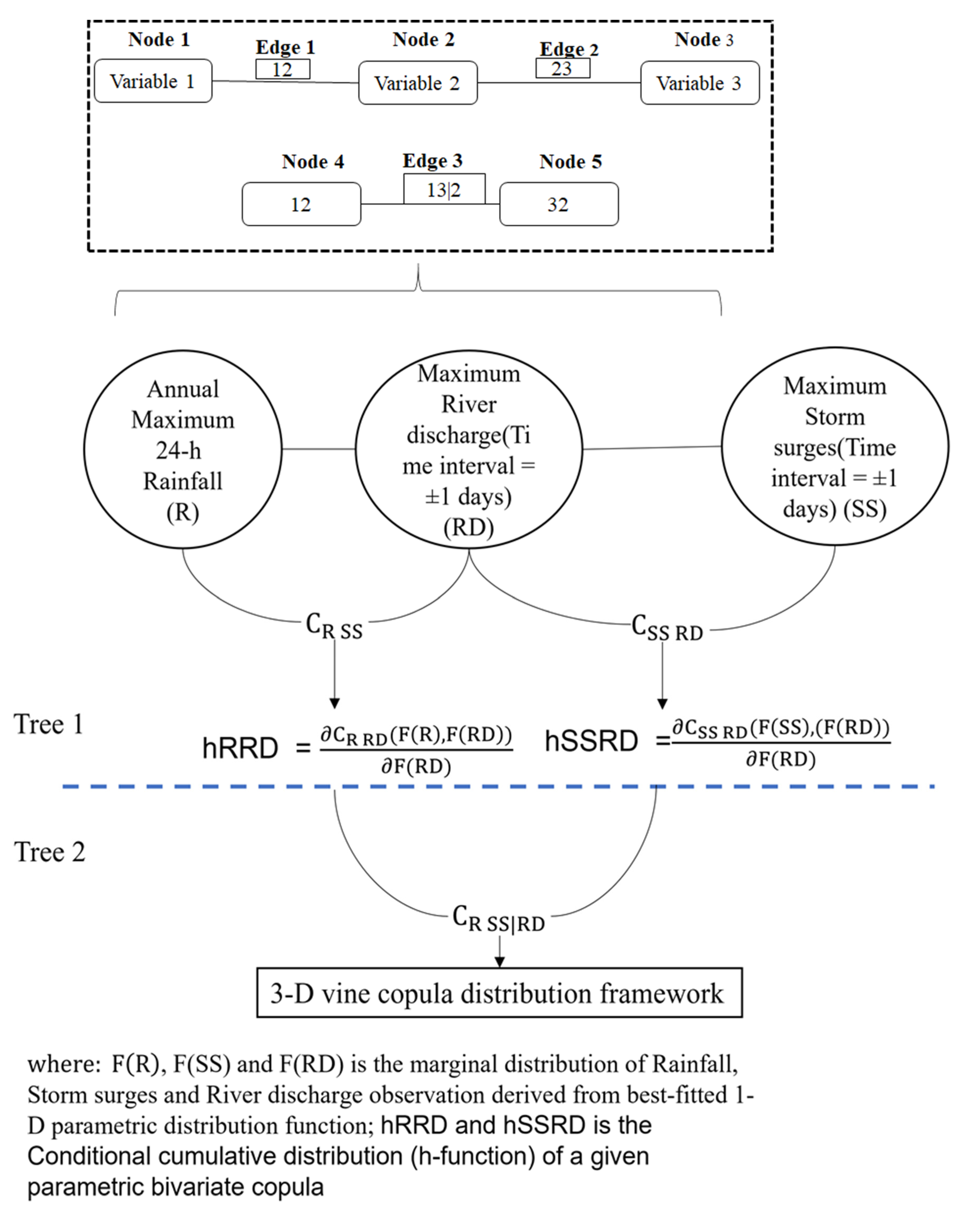
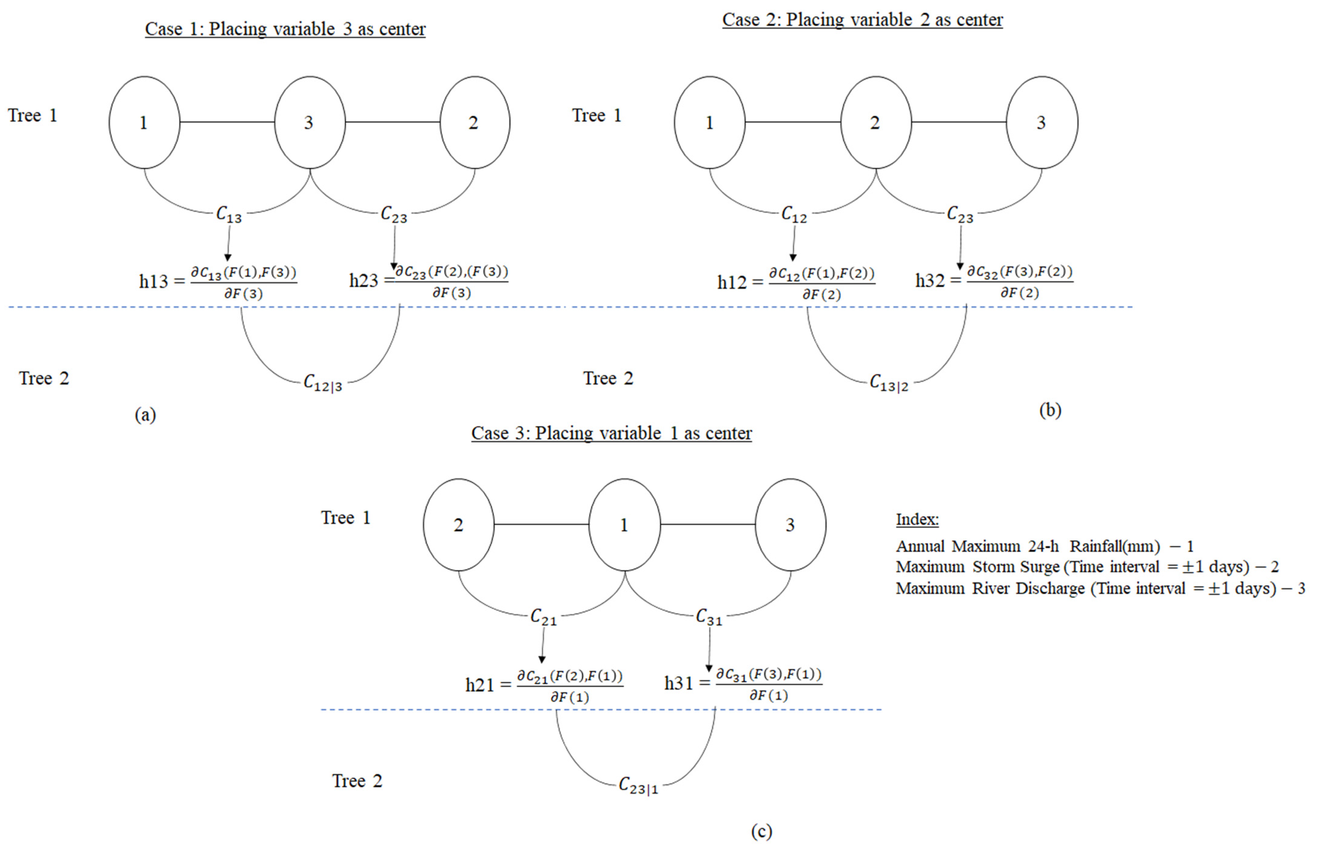
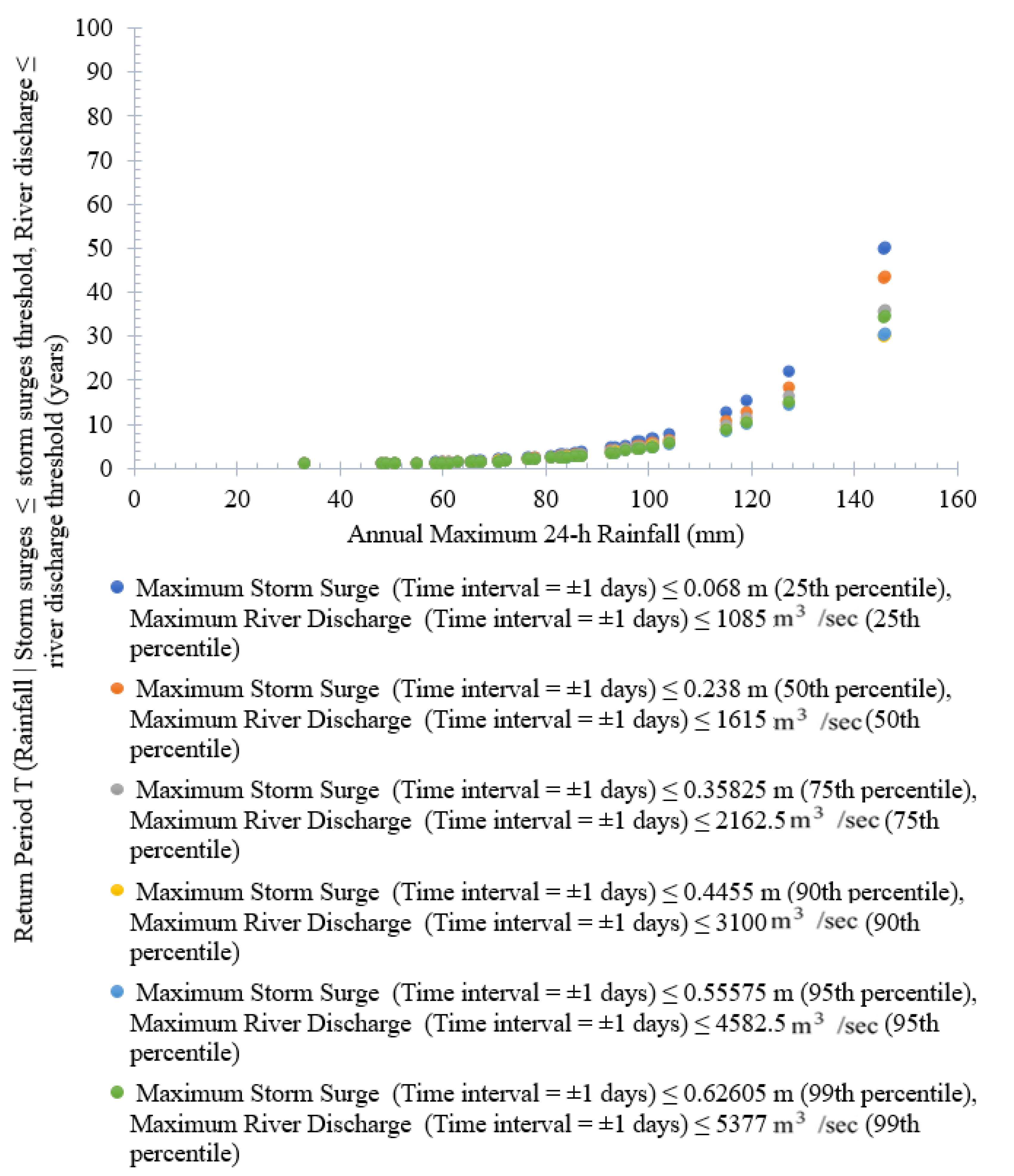
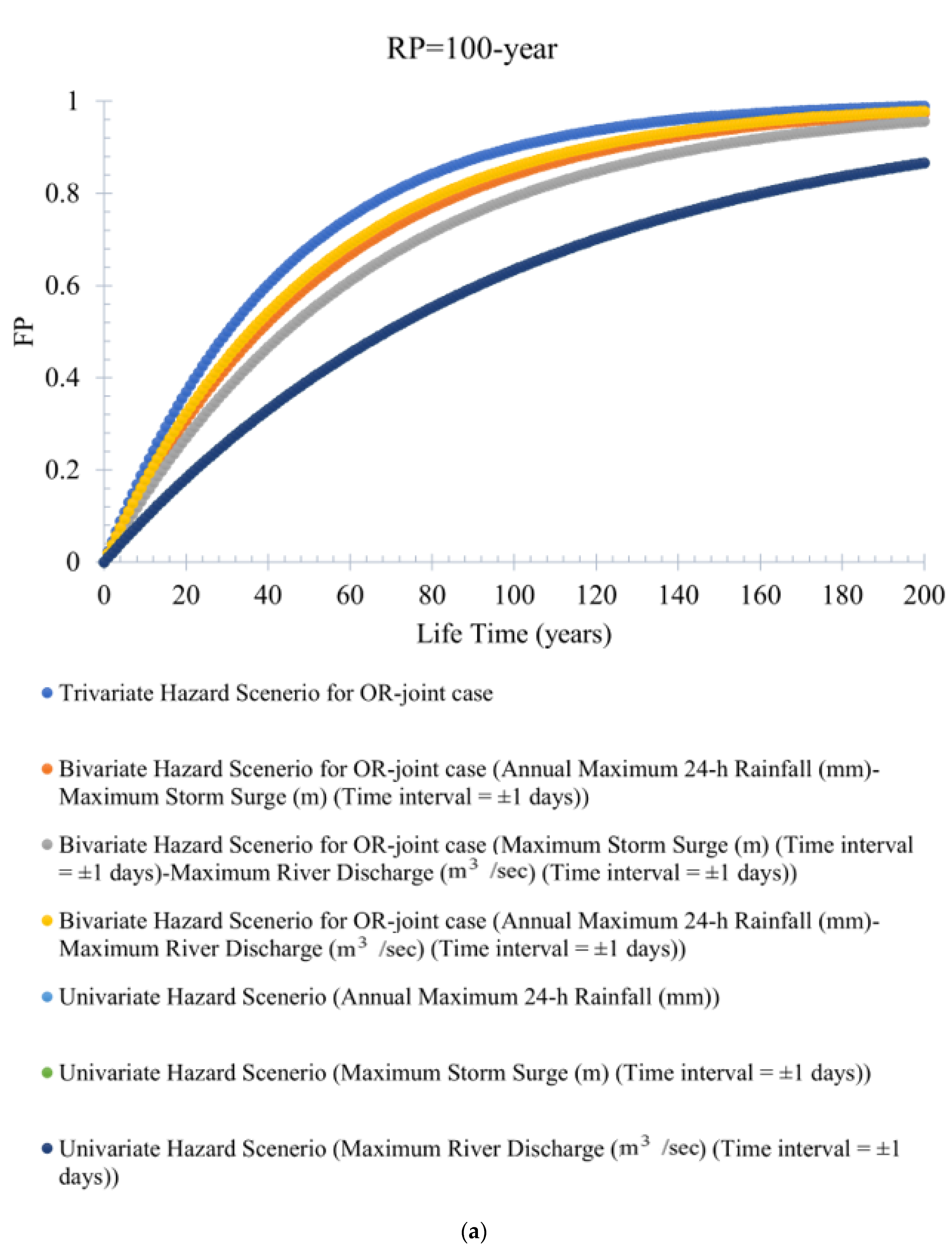
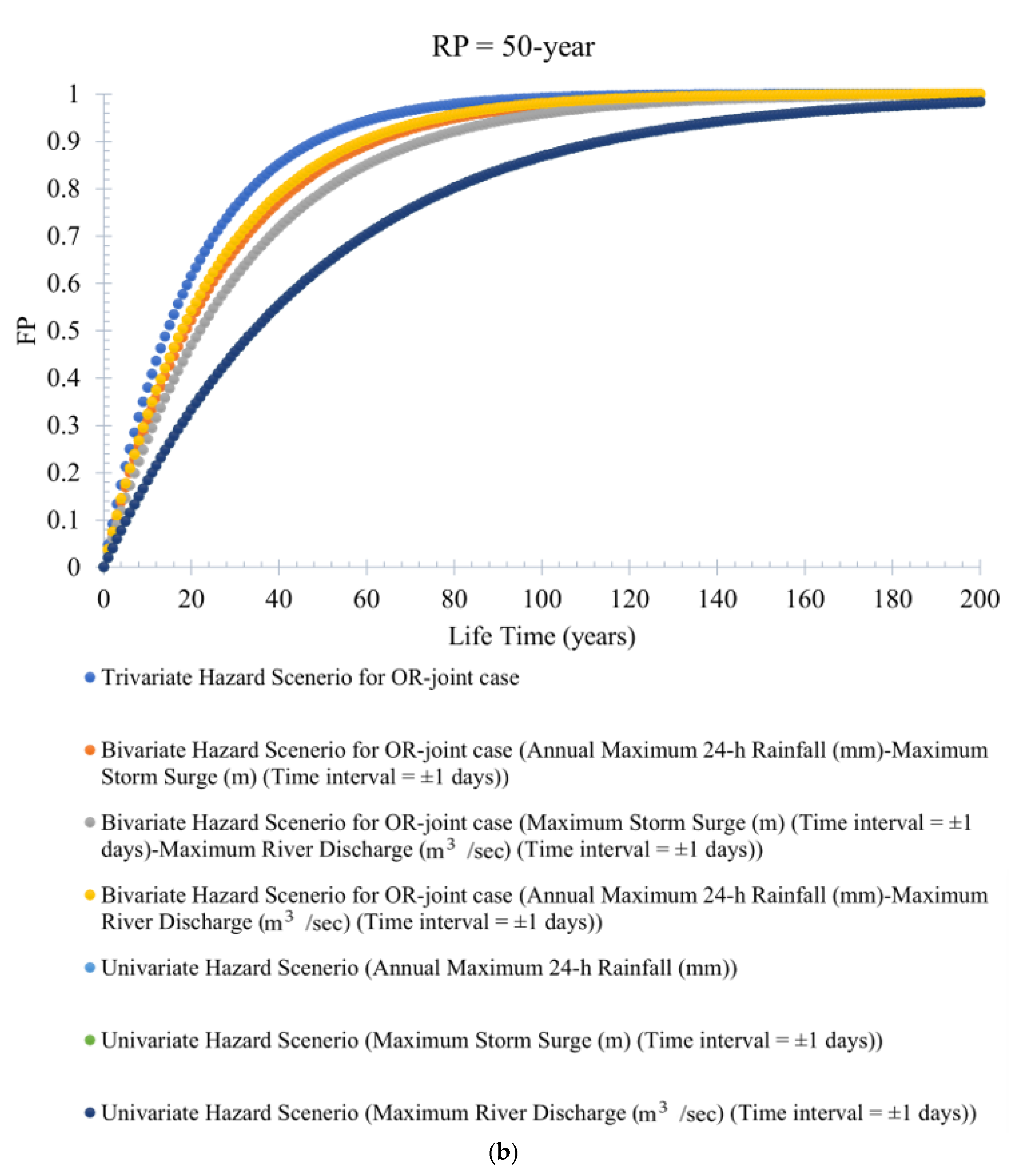
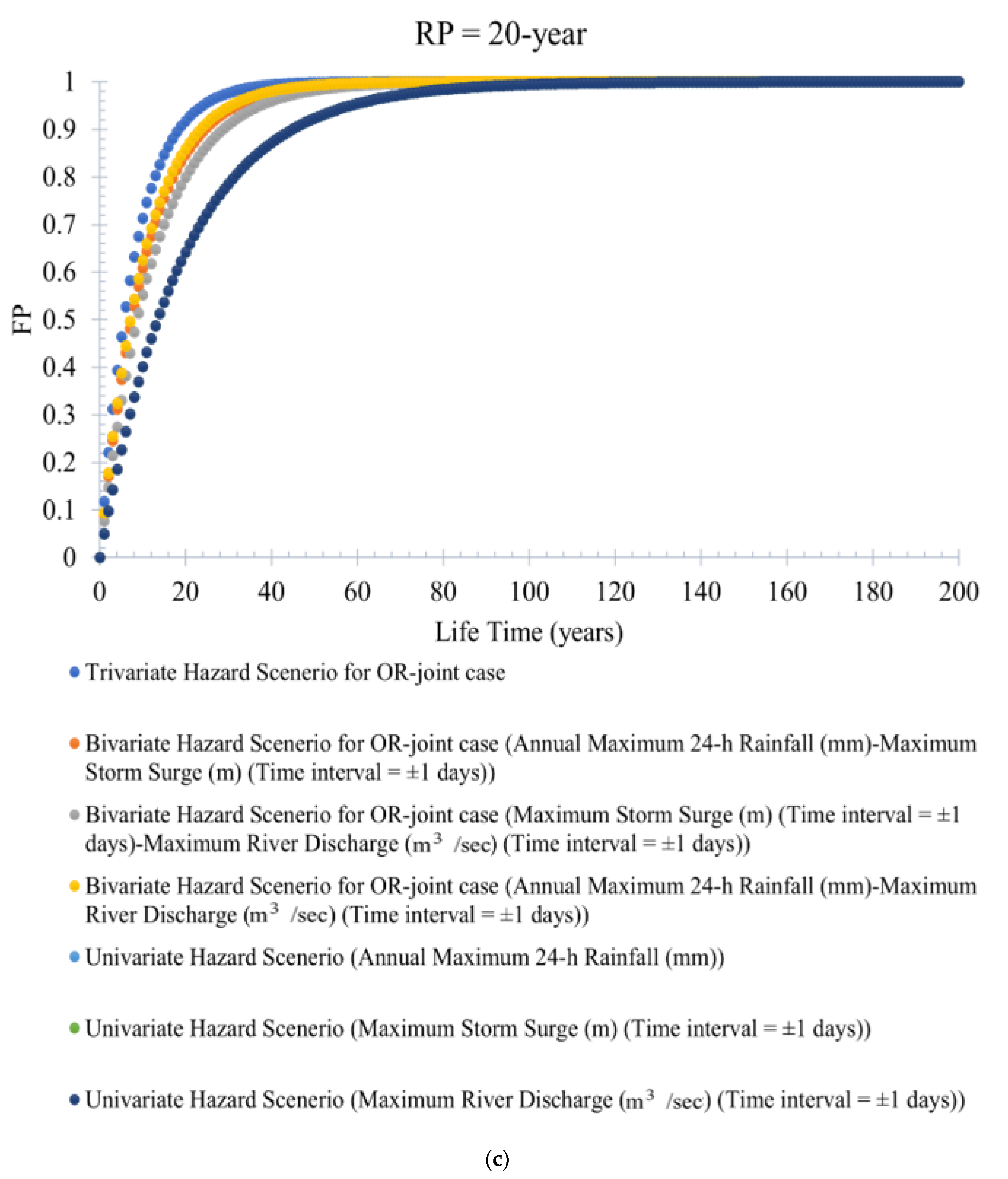
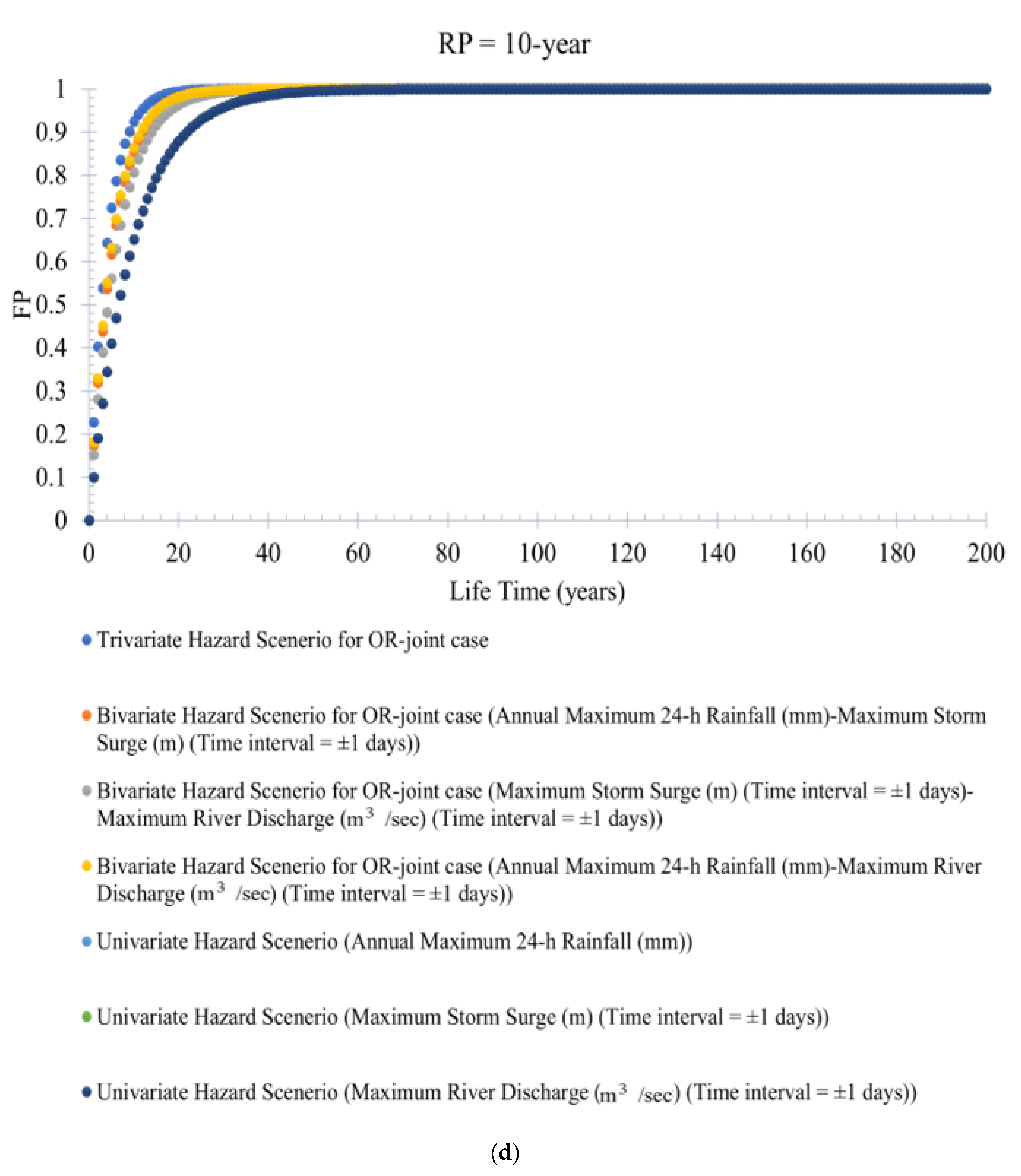
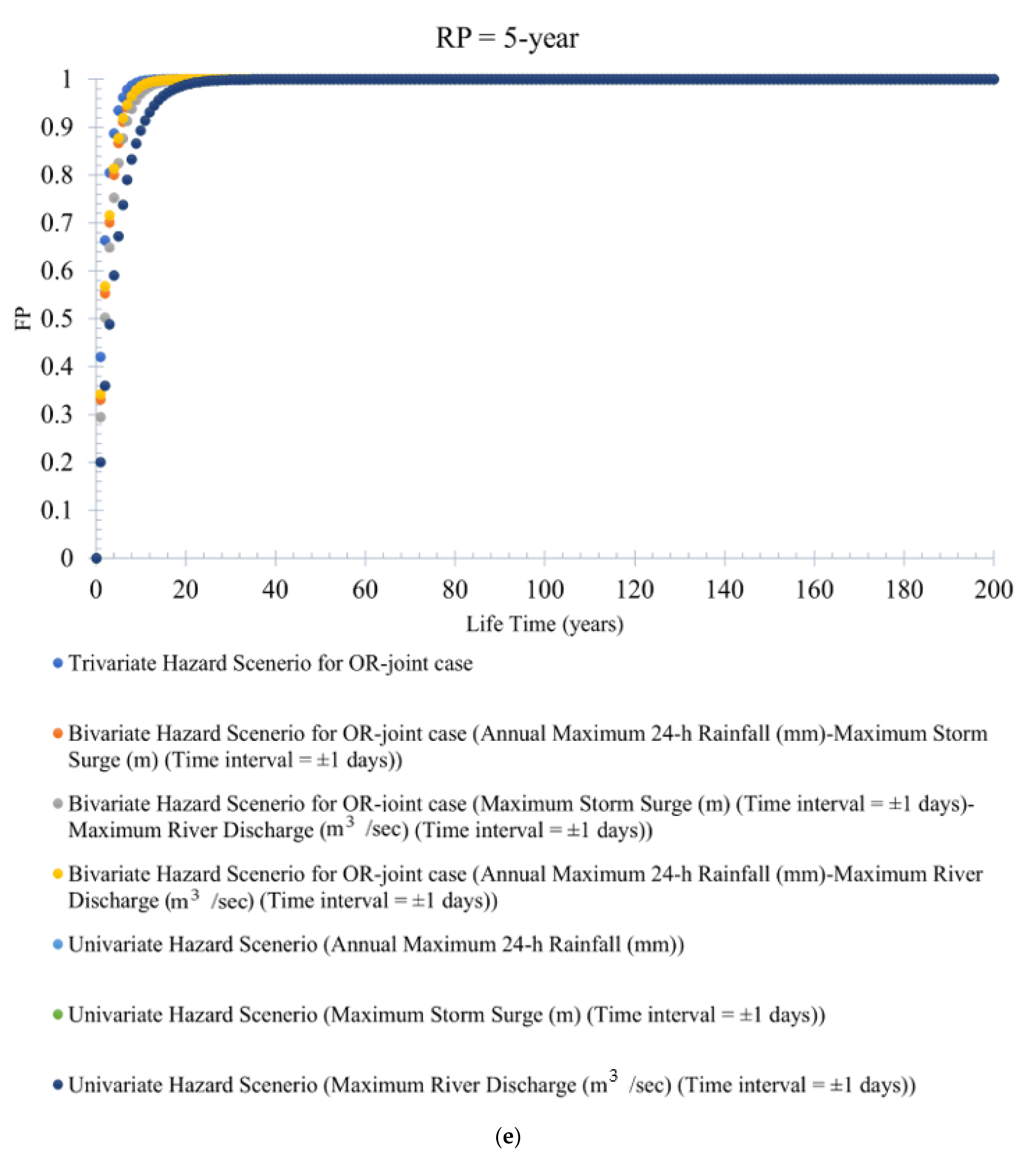
Table 1.
Measures of dependency strength between flood characteristics.
| Dependency Measure Statistics | Compound Flood Variables | ||
|---|---|---|---|
| Annual Maximum 24-h Rainfall-Maximum Storm Surge (Time Interval = ±1 Days) | Maximum Storm Surge (Time Interval = ±1 Days)—Maximum River Discharge (Time Interval = ±1 Days) | Annual Maximum 24-h Rainfall-Maximum River Discharge (Time Interval = ±1 Days) | |
| Pearson | 0.301 | 0.469 | 0.118 |
| Kendall | 0.208 | 0.341 | 0.094 |
| Spearman | 0.297 | 0.504 | 0.122 |
Note: The correlation coefficients are measured at a significance level of 0.05 or confidence interval 0.95. The computed p-value of all the above correlation measures is less than 0.05, i.e., significance correlation exhibited between variable of interest.
Table 2.
Overall summary table of fitted 3D vine copula frameworks constructed via permutation of conditioning variables (flood variable centred at the selected D-vine structure).
Table 2.
Overall summary table of fitted 3D vine copula frameworks constructed via permutation of conditioning variables (flood variable centred at the selected D-vine structure).
| Vine Structure (Conditioning Variable) | Tree Level | Flood Attribute Pairs | Most Parsimonious or Best-Fitted Copula | Log-Likelihood (LL) | Akaike Information Criterion (AIC) | Bayesian Information Criterion (BIC) | ||
|---|---|---|---|---|---|---|---|---|
| Case 1 (1-3-2) * | is placed in the center) | Tree 1 | 1-3 (Rain-River discharge) | Survival BB7 (Rotated BB7 180 degrees) | 9.53788 | −10.87909 | −3.564521 | |
| 3-2 (Storm surge-River discharge) | Gumbel | = par= 1.554 | ||||||
| Tree 2 | 12|3 | Clayton | 0.3688 | |||||
| Case 2 (1-2-3) | placed in the center) | Tree 1 | 1-2 (Rain—Storm surge) | BB7 (Joe-Clayton) | 8.194824 | −6.389647 | 2.75356 | |
| 2-3 (Storm surge—River discharge) | Gumbel | = par = 1.554 | ||||||
| Tree 2 | 13|2 | Rotated BB8 270 degrees | = par = −1.083(delta) = par2 = −1.000 | |||||
| Case 3 (2-1-3) | D-vine structure 1 (Variable 1 or Annual maximum 24-h rainfall placed in the center) | Tree 1 | 2-1 (Storm surge-Rain) | BB7 (Joe-Clayton) | 9.34687 | −8.693741 | 0.449466 | |
| 3-1 (River discharge-rainfall) | Survival BB7 (Rotated BB7 180 degrees) | |||||||
| Tree 2 | 23|1 | Frank | 3.689 |
Note: Case 1 (Maximum river discharge (Time interval = ) is a conditioning variable, indicated by bold letter with an asterisk *) is the best description of the 3D vine copula dependence structure with minimum value of AIC and BIC test statistics (highest log-likelihood of the model).
Table 3.
Estimation of dependence parameters of the fitted 3D FNA copulas and comparing their performance with selected best-fitted D-vine copula (D-vine structure 1).
Table 3.
Estimation of dependence parameters of the fitted 3D FNA copulas and comparing their performance with selected best-fitted D-vine copula (D-vine structure 1).
| Trivariate Distribution Framework | Copula Function | Log-Likelihood (LL) | Akaike Information Criterion (AIC) | Bayesian Information Criterion (BIC) | |
|---|---|---|---|---|---|
| Parametric 3D Vine or Pair-Copula Construction (PCC) | D-Vine Copula * | 9.53788 | −10.87909 | −3.564521 | |
| Estimated Parameters | Log-Likelihood (LL) | ||||
| Asymmetric or fully nested Archimedean (FNA) framework (parametric marginals) | Gumbel copula | 9.063 | −0.408 | 3.248 | |
| Clayton copula | 5.627 | 0.544 | 4.201 | ||
| Frank copula | 8.594 | −0.302 | 3.355 | ||
Note: First, the Gumbel copula is recognised as the best-fitted among the fitted 3D FNA copulas. D-vine copula (indicated by bold letter with an asterisk *) exhibited minimum value of information criteria-based goodness-of-fit (GOF) test statistics (i.e., AIC and BIC), also highest value of log-likelihood of the fitted model compared to nested Gumbel copula. Thus, selected as the best-fitted distribution in the trivariate joint probability analysis of compound flooding events.
Table 4.
Examining the reliability of the developed 3D parametric vine copula structure vs. 3D FNA Gumbel–Hougaard copula by comparing Kendall’s correlation coefficient estimated using the generated random samples (size N = 1000) obtained from the above-selected model with Empirical Kendall’s values estimated from historical observations.
| Flood Attribute Pairs | |||
|---|---|---|---|
| Annual maximum 24-h rainfall (mm)-Maximum storm surge (m) (Time interval = | 0.207 | 0.192 | 0.196 |
| Maximum storm surge (m) (Time interval = | 0.341 | 0.358 | 0.342 |
| Annual maximum 24-h rainfall (mm)—Maximum river discharge (m3/s) (Time interval = | 0.093 | 0.156 | 0.120 |
Note: The selected D-vine copula structure regenerates the dependency of historical flood characteristics more effectively.
Table 5.
Univariate, bivariate and trivariate joint return periods (JRPs) estimated for various combinations of selected flood characteristics.
Table 5.
Univariate, bivariate and trivariate joint return periods (JRPs) estimated for various combinations of selected flood characteristics.
| Flood Quantiles Estimated Using the Inverse of the Best-Fitted Marginal Cumulative Distribution Functions (CDFs) | Bivariate Joint Return Periods (JRPs) | Trivariate Joint Return Periods (JRPs) Estimated Using the Best-Fitted D-Vine Copula Structure (Case 1, Refer to Table 2) | |||||||||
|---|---|---|---|---|---|---|---|---|---|---|---|
| Return Period (RPs) (Years), T | Annual Maximum 24-h Rainfall (R) (mm) | Maximum Storm Surge (m) (SS) (Time Interval = ±1 Days) | Maximum River Discharge (RD) (m3/s) (Time Interval = ±1 Days)) | ||||||||
| 5 | 102.90 | 0.145 | 2412.582 | 3.01 | 14.58 | 2.91 | 17.43 | 3.40 | 9.40 | 2.380 | 19.31 |
| 10 | 120.68 | 0.221 | 3374.429 | 5.72 | 39.47 | 5.52 | 52.75 | 6.60 | 20.57 | 4.40 | 50.98 |
| 20 | 138.75 | 0.284 | 4685.815 | 11.18 | 94.71 | 10.71 | 150.38 | 13.01 | 43.13 | 8.52 | 133.76 |
| 50 | 163.73 | 0.354 | 7215.067 | 27.59 | 265.73 | 26.17 | 557.63 | 32.26 | 110.99 | 21.48 | 964.97 |
| 100 | 183.68 | 0.401 | 10,005.067 | 54.98 | 551.45 | 51.80 | 1435.13 | 64.35 | 224.15 | 43.90 | 1280 |
| 200 | 204.69 | 0.444 | 13,886.119 | 109.78 | 1121.95 | 102.87 | 3575.25 | 128.52 | 450.51 | 79.19 | 1002.40 |
| 500 | 234.24 | 0.497 | 21,446.821 | 274.22 | 2830.45 | 255.57 | 11,454.75 | 321.05 | 1129.56 | 188.38 | 1596.42 |
| 1000 | 258.04 | 0.533 | 29,822.745 | 548.27 | 5678.59 | 509.45 | 26,954.17 | 641.93 | 2261.42 | 364.00 | 2508.15 |
Publisher’s Note: MDPI stays neutral with regard to jurisdictional claims in published maps and institutional affiliations. |
© 2022 by the authors. Licensee MDPI, Basel, Switzerland. This article is an open access article distributed under the terms and conditions of the Creative Commons Attribution (CC BY) license (https://creativecommons.org/licenses/by/4.0/).
Share and Cite
MDPI and ACS Style
Latif, S.; Simonovic, S.P. Parametric Vine Copula Framework in the Trivariate Probability Analysis of Compound Flooding Events. Water 2022, 14, 2214. https://doi.org/10.3390/w14142214
AMA Style
Latif S, Simonovic SP. Parametric Vine Copula Framework in the Trivariate Probability Analysis of Compound Flooding Events. Water. 2022; 14(14):2214. https://doi.org/10.3390/w14142214
Chicago/Turabian StyleLatif, Shahid, and Slobodan P. Simonovic. 2022. "Parametric Vine Copula Framework in the Trivariate Probability Analysis of Compound Flooding Events" Water 14, no. 14: 2214. https://doi.org/10.3390/w14142214
Note that from the first issue of 2016, this journal uses article numbers instead of page numbers. See further details here.