
Assessment of Uncertainty in Grid-Based Rainfall-Runoff Model Based on Formal and Informal Likelihood Measures


1
Department of Advanced Science and Technology Convergence, Kyungpook National University, 2559 Gyeongsangdaero, Sangju 37224, Gyeongbuk, Korea
2
Department of Hydro Science and Engineering Research, Korea Institute of Civil Engineering and Building Technology, 283 Goyangdaero, Ilsanseogu, Goyangsi 10223, Gyeonggido, Korea
*
Author to whom correspondence should be addressed.
Water 2022, 14(14), 2210; https://doi.org/10.3390/w14142210
Submission received: 4 May 2022
/
Revised: 25 June 2022
/
Accepted: 8 July 2022
/
Published: 13 July 2022
(This article belongs to the Section Hydrology)
Abstract
:Damage prevention from the local storms and typhoons in Korea, the development of a rainfall-runoff model reflecting local geological, meteorological and physical characteristics is necessary. The accuracy of the rainfall-runoff model is influenced by the various uncertainty factors that can occur in the modeling processes, including input data, model parameters, modeling simplification, and so on. Thus, the objectives of this study are (1) to estimate runoff for two rainfall events using Grid Rainfall-Runoff Model (GRM); (2) to quantify the uncertainty of the GRM model using the Generalized Likelihood Uncertainty Estimation (GLUE) method, and (3) to assess the uncertainty ranges of the GRM based on different likelihood functions. For this, two rainfall events were implemented to the GRM in the Cheongmicheon watershed, and informal likelihood functions (LNSE, LPBIAS, LRSR, and LLOG) based on the fitness indices (NSE, PBIAS, RSR, and Log-normal) were used for uncertainty analysis and quantification using GLUE method. As a result, the GRM parameters varied according to the different rainfall patterns even in the same watershed. In addition, among the GRM parameters, the CRC (Channel Roughness Coefficient) and CSHC (Correction factor for Soil Hydraulic Conductivity) characteristics are the most sensitive. Moreover, this study showed that the uncertainty range of the GRM model can be changed with the subjective selection of likelihood functions and thresholds. The GRM model is open source and has good accessibility. Especially, this open-source model allows various approaches to disaster prevention plans such as flood forecasting and flood insurance policies. In addition, if the parameter range of GRM is quantified and standardized at domestic watersheds, it is expected that the reliability of the rainfall-runoff simulation can be increased by the reduction of the uncertainty factors.
1. Introduction
Unpredictable changes in weather have frequently occurred in recent years due to climate change. These abnormalities have led to numerous of natural disasters worldwide, indicating an urgent need to reduce and mitigate such disasters. Recent cases of natural disasters, such as flooding, in South Korea have exhibited damage patterns different from the long-lasting monsoons of the past, resulting in enormous damage due to localized heavy rainfall. Predicting damage due to runoff from localized heavy rainfall is challenging. Since there is an increasing risk of this runoff worldwide, however, numerous studies have been conducted to ensure the accuracy of predictions regarding short-term rainfall runoff [1,2,3,4,5].
Various hydrological models are used to predict the short-term rainfall-runoff process. Rainfall-runoff models, which reflect the runoff characteristics of watersheds, are widely used. These runoff characteristics can be conceptually or physically represented, and recent developments in geographic information systems have enabled the frequent application of physical models. In particular, despite various interpretations depending on its grid size, a distribution model can represent the runoff characteristics of an entire watershed by combining grids, as each grid (corresponding to a certain part of the watershed) includes runoff characteristics. If the combination of grids in a physical model accurately reproduces the actual hydrological phenomenon of the watershed by using the governing equation, and the parameters constituting the governing equation perfectly reflect the physical hydrological characteristics of the watershed, such a model could accurately predict short-term runoff without calibration or validation. However, the governing equation includes many uncertainties, as it interprets hydrological phenomena through parameters, simplifying natural phenomena in the process. Thus, more accurate prediction could be ensured by analyzing the uncertainty of the employed parameters [6,7,8].
In an event-based rainfall-runoff model, the parameters constituting the model depend on the type of rainfall. For example, the parameter reflecting the initial saturation of soil is greatly affected by the type of rainfall, which in turn affects the prediction of runoff [9,10]. It is difficult to perform calibration and validation for the model, as the rainfall, which provides the input data, continuously changes over time. However, the parameters that have been calibrated are frequently applied to predict other rainfall events [11]. A parameter corrected for one event may deviate from the adjusted confidence interval in its application to another rainfall event, so it may be a cause of uncertainty [12]. Thus, we can seek understanding of the uncertainties in parameters depending on the model prediction results by applying various types of rainfall to the model to secure its reliability [13].
Various methods have been used to analyze the uncertainties in rainfall-runoff models: Monte Carlo simulation (MCS) [6,14], Latin hypercube sampling [15,16], state-space filtering [17,18], and first-order second-moment [19,20]. In particular, uncertainty analysis of these models has been widely conducted by utilizing the various likelihood estimators, in which the relationship between model results and observations by parameter combinations is defined as a Bayesian-based function [21].
Compared to other uncertainty analyses, generalized likelihood uncertainty estimation (GLUE) [6] is a flexible and simple uncertainty analysis technique that can apply both formal and informal likelihood. For this reason, it is among the most widely used methods for uncertainty analysis in many rainfall-runoff models [22]. The parameters of a rainfall-runoff model generated from the prior distribution in a GLUE simulation process based on Bayes’s theorem can be utilized to form a posterior distribution in the uncertainty analysis process by the critical point for the likelihood, which is obtained from the relationship between the model results and the observation values. The posterior distribution of these parameters provides important information that can accurately link rainfall, which is the input data, and runoff, which is the model prediction value. However, this posterior distribution may vary depending on the type and threshold of likelihood, and this subjective selection may become a negative factor in ensuring consistent analysis of uncertainty in a rainfall-runoff model. Thus, for a smooth uncertainty analysis, it is important to find a likelihood that can best reflect the error characteristics between the predicted value and the observed value of the rainfall-runoff model by the combination of parameters [21]. There has been controversy over the use of formal and informal likelihood in the selection of likelihood for the analysis of uncertainty in rainfall-runoff models [18,23,24]. Typically, formal likelihood is applicable to the uncertainty analysis, in which the statistical structure of error is established. However, because it is difficult to quantify the individual errors that may occur in the input data and the model structure, informal likelihood can be usefully applied to uncertainty analysis, in that uncertainty analysis is frequently conducted after combining these individual errors into a total error term [25].
Uncertainty may occur when predicting runoff by applying the parameters of the grid-based rainfall-runoff model (GRM) corrected for one rainfall event to another rainfall event. Furthermore, the results of uncertainty analysis may vary depending on subjective selection of likelihood. Thus, this study evaluated how the type of rainfall and the selection of likelihood affect the parameters of the GRM. For this purpose, an uncertainty analysis of parameters in a rainfall-runoff model using GLUE was conducted to compare and analyze the posterior distribution of parameters for two rainfall events. In addition, this study conducted uncertainty analysis utilizing three values of informal likelihood, aiming to determine their effect on the model results.
2. Materials and Methods
2.1. Study Area
The Cheongmicheon Watershed is part of the Han River water system in South Korea, which is an important basin supplying water to Seoul and Incheon. It is located upstream of the Namhan River. The watershed is showed in Figure 1. In addition, the Cheongmicheon Watershed is a test basin selected by the International Hydrological Program to explore the hydrological water cycle in South Korea. In this regard, various hydrological and water-quality studies have been conducted because the hydrological and topographical data on the Cheongmicheon Watershed have been well established over a relatively long term.
2.2. Grid-Based Rainfall-Runoff Model (GRM) Definition
The GRM was developed as a physically based distribution model to simulate runoff for rainfall events [26]. The GRM can be utilized to predict surface and lateral runoff, infiltration, and subsurface flow due to rainfall events, and to evaluate the effect of rainfall on the flow rate adjusted by artificial structures at the watershed. Moreover, the GRM is designed to visualize a watershed by using geospatial data composed of a grid format, and to use average rainfall or distributed rainfall data in grid format. In the GRM, the kinetic wave equation is applied to analyze surface and lateral flow, and infiltration is calculated through the Green-Ampt model. Each grid constituting the watershed is set as a control volume, and the finite volume method is applied to perform a runoff simulation. The governing equations of the GRM are represented as Equations (1)–(3) [27].
In the equations, h is flow depth, q is flow rate per unit width, r is rainfall intensity, f is infiltration rate, qr is return flow, y is the width of control volume, A is cross-sectional area, Q is discharge, qL is lateral flow, qss is subsurface flow, qb is baseflow, S0 is surface slope, and Sf is friction slope.
2.3. Rainfall-Runoff Analysis
A rainfall-runoff simulation using the GRM requires rainfall data and a map spatially representing land use, soil type, and elevation. Furthermore, observational runoff data are needed for calibration and validation of the GRM model. This study utilized 90 m * 90 m Digital Elevation Model of the National Geographic Information Institute (https://www.ngii.go.kr; accessed on 10 February 2022), as well as the precise soil map and soil depth data of the Rural Development Administration (http://www.naas.go.kr; accessed on 10 February 2022), and the large classification land use map in the Environmental Geographic Information System of the Ministry of Environment (ME, http://www.me.go.kr; accessed on 10 February 2022), as shown in Figure 3.
In addition, this study used the meteorological data of 11 meteorological stations of the ME located near the target area of this study: Beopcheon, Samjuk, Seolseong, Saenggeuk, Anseong, Yeoju Bridge (Yeoju), Oryu, Wonsam, and Eumseong, Namgok, and Geumdang Elementary School (Taepyeong) stations. To consider the spatial influence on meteorological data, this simulation was performed by calculating the Thyssen weights through the Thiessen network depending on the location of the station and utilizing the average rainfall of the corresponding area. The general formula for obtaining the Thiessen network is shown in Equation (4).
where , N, Ai, and Pi refer to the average rainfall in the watershed, the number of stations, the effect area for each station, and the measured precipitation for each point, respectively.
The highest Thiessen weight was 26.13% at the Samjuk Meteorological Station, exhibiting the greatest influence. The ratios of weights for each station are ranked in the order of Samjuk, Taepyeong, Beopcheon, Yeoju, Wonsan, Seolseong, Saenggeuk, Eumseong, Namgok, Angseong, and Oryu. Table 1 summarizes the weights of each station affecting the Cheongmicheon Watershed.
The rainfall events applied in this study had rainfall higher than 35.6 mm, which was the hourly rainfall of the Cheongmicheon Watershed for 50 years. For the validation of the GRM model, this study utilized the data on the flow rate per 10 min from Janghowon Bridge of the Han River Flood Control Office of the ME, a flow observation station in the Cheongmicheon Watershed. In addition, the flow data for validation were collected during the period until the flow rate analyzed in the model returned to the normal flow rate. Furthermore, regarding each period and event, data were collected; the comparative validation periods are presented in Table 2.
2.4. Uncertainty Analysis Using Generalized Likelihood Uncertified Estimation (GLUE)
The method for uncertainty analysis using GLUE is based on the Hornberger-Spear-Young global sensitivity analysis [28,29], and a combination of random variables, which are generated from a specific probability density function (PDF) within the feasible range, is applied to the MCS. In GLUE, it is essential to select a behavioral model that matches the combination of random variables. The results from the MCS using the combination of random variables are weighted by a likelihood measure. Typically, a likelihood measure is employed to determine how well a simulated result fits an observation. The concept of GLUE is based on the Bayesian equation (Equation (5)), and an informal likelihood function can be utilized to estimate the likelihood measure used in GLUE [30].
where θ, ε, and c refer to the parameter combination, the error between the observed value (O) and the simulated value, and the scaling constant, respectively. P[θ|O], P[θ], and P[θ] refer to the posterior PDF, likelihood, and prior PDF, respectively.
A likelihood measure represents the goodness of fit (GoF) between observed values and model values, and typically, high likelihood measures indicate high GoF. A likelihood measure is divided into a behavioral model (or accepted dataset) and a nonbehavioral model (or non-accepted dataset), depending on the threshold value. A behavioral model refers to a combination of variables, in which the likelihood measure satisfies the threshold value. Here, a combination of variables refers to a combination of parameters in the model randomly selected within a given range, and the uncertainty calculation generates a cumulative density function (CDF) by weighting only the likelihood measure derived by the behavioral model. The median of the CDF is typically utilized as a representative value of the model’s predicted results, and the uncertainty is quantified by a 90% confidence interval selected with 5% and 95% confidence levels [6,24,31].
The GLUE method is utilized to analyze uncertainty using MCS based on Bayesian theory (Equation (6)). The likelihood used in GLUE can be determined by several likelihood functions. This study selected three GoF indicators, namely Nash-Sutcliffe efficiency (NSE), PBIAS, and rank-sum ratio (RSR), which are formal likelihood estimators, to calculate the likelihood function, as well as a log-normal index, which is the informal likelihood.
where M, y, P(M), P(M|y), and L(y|M) are a combination of model parameters, a set of observed values, a prior distribution of the model, posterior distribution, and likelihood by model evaluation, respectively.
The purposes of the GLUE method are to classify a behavioral model among the combinations of random variables, weight the results from MCS using the combinations of random variables by likelihood, and determine how suitable the simulated results are for the observed values.
NSE is Nash–Sutcliffe model efficiency coefficient that determines the relative magnitude of residual variance (“noise”) in comparison to the variance of the measured data (“information”) [32]. NSE is calculated as shown in Equation (7).
where N refers to the number of observations, Ot and Pt refer to the actual and predicted flow at time t, and
refers to the average value of the actual flow.
Percent bias (PBIAS) refers to the average trend of simulated data and the degree to which it is larger or smaller than that of the observed data [33]. The optimal value of PBIAS is 0.0, and low values indicate that the model simulation is accurate. Positive values correspond to underestimation bias in the model, whereas negative values correspond to overestimation bias in the model, which are represented as shown in Equation (8).
where N refers to the number of data, and and refer to the actual and predicted flow at time t.
The RSR (RMSE-observations standard deviation ratio) standardizes the root mean square error (RMSE) by utilizing the observed standard deviation [34] and combines additional information with the error index recommended by Legates and McCabe [35]. Simply, this means we constrained the values between 0–1. The RSR is calculated as the ratio of the RMSE to the standard deviation of the measured data, as shown in Equation (9).
where N refers to the number of data, and refer to the actual and predicted flow at time t, and refers to the average value of the actual flow.
Log-normal (log-likelihood function) is the log of the likelihood function, measuring the GoF between model parameters and observed data through the natural logarithm, for convenience in calculating the maximum likelihood estimate. Since the behavioral model can be determined by selecting a part of the upper values if there is no criterion for the threshold, as in log-normal, this study has assumed that the upper 30% values represent the behavioral model [6,36]. Log-normal is shown in Equation (10).
where N refers to the number of observed values, σ2 refers to the variance of the simulated and observed values, as shown in Equation (11), and εi(θ) refers to the vector value of the residual, which corresponds to the difference between the simulated and observed values at time t, as indicated in Equation (12).
The likelihood measure was analyzed by utilizing the previously described four GoF indices: NSE, PBIAS, RSR, and log-normal. Typically, as the likelihood value becomes higher, the GoF is determined to be higher. Thus, this study, to calculate the likelihood measure, conducted an analysis by applying Equation (13) corresponding to NSE, Equation (14) corresponding to an inverse of absolute value of PBIAS, Equation (15), a formal likelihood function corresponding to a reciprocal of the RSR, and Equation (16), an informal likelihood function corresponding to log-normal (log-likelihood function).
The analysis proceeded by dividing into nonbehavioral models and behavioral models according to the likelihood measure values obtained by using Equation (13) through (16) [24,31]. Here, the behavioral model refers to a combination of variables randomly selected within the given range, and the uncertainty calculation is performed by using the behavioral model, in which a CDF is generated by utilizing weights for each likelihood. A quantitative analysis was conducted with a 90% confidence interval by using the 5% and 95% confidence interval analysis utilizing the CDF [31].
2.5. Automation Analysis and Parameter Setting of the GRM
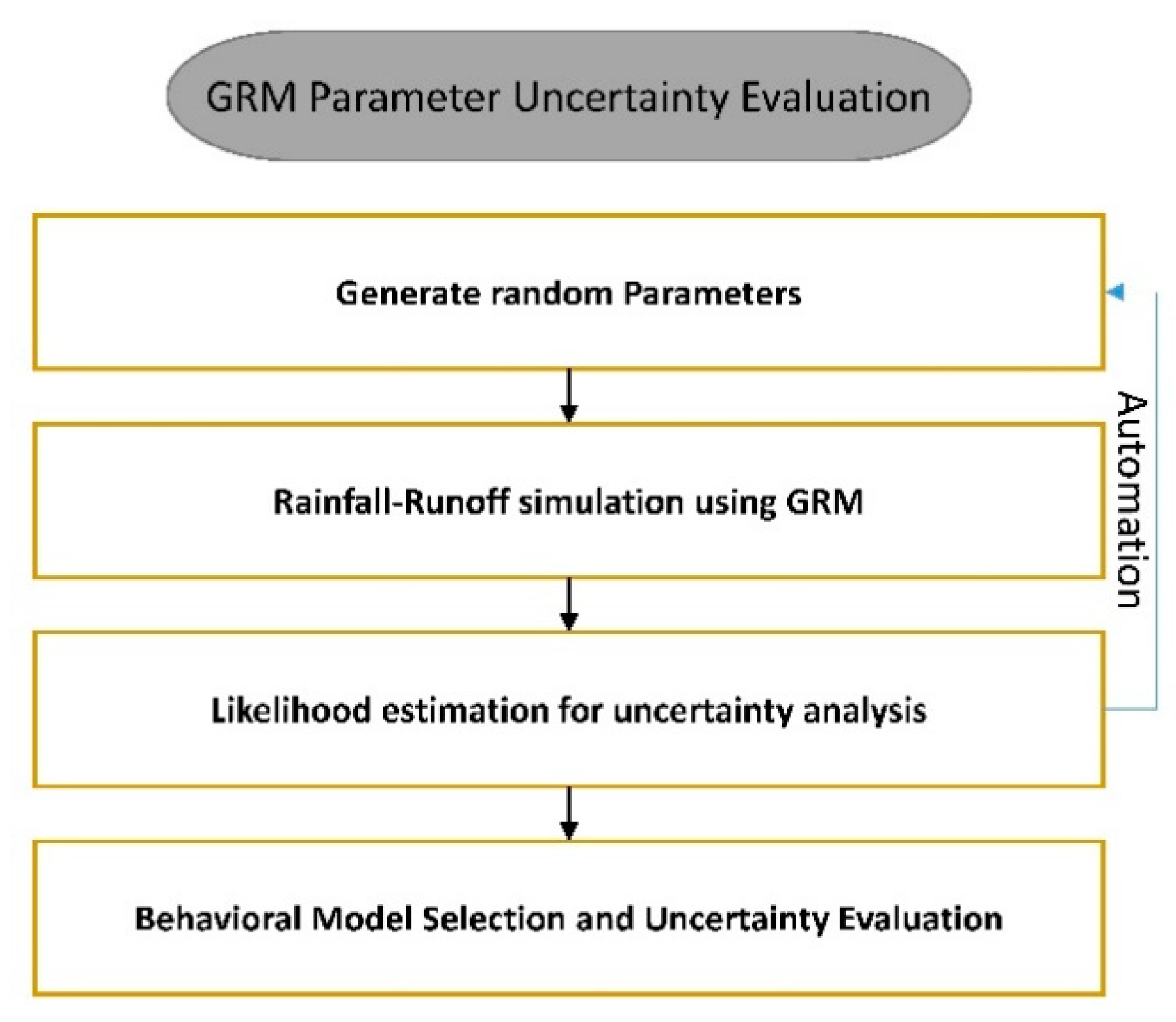
To evaluate the uncertainty of GRM parameters, a combination of random parameters was generated through MCS within each range for eight parameters out of nine in the GRM. Automated coding using Python was applied to the analysis in the order of rainfall-runoff simulation using the GRM, likelihood calculation for uncertainty analysis, and selection and evaluation of the behavioral model; a flowchart is provided in Figure 4.
The applied parameters were IniSaturation, MinSlopeOF, ChRoughness, CalCoefLCRoughness, CalCoefSoilDepth, CalCoefPorosity, CalCoefWFSuctionHead, and CalCoefHydraulicK, and the range for each parameter was determined by setting the minimum and maximum ratios for each GRM parameter [27]. The range and definition of each parameter are presented in Table 3. In addition, regarding the target watershed, simulations were performed 10,000 times for each of the two events, and additional simulations on the primary analysis results were performed 5000 times within the range that satisfied the likelihood. Table 3 shows the allowable range for parameters.
3. Results
3.1. Distribution of Parameters According to Likelihood
Analyzing the distribution of the formal likelihood calculated through the log-normal function, and the informal likelihood depending on the three types of NSE, PBIAS, and RSR, behavioral models were determined with the threshold values of the upper 30% for formal likelihood, and with the cases where the NSE value was 0.65 or higher [37], PBIAS < |25|, and RSR < 0.7 [34].
3.1.1. Event 1 Dotty Plot
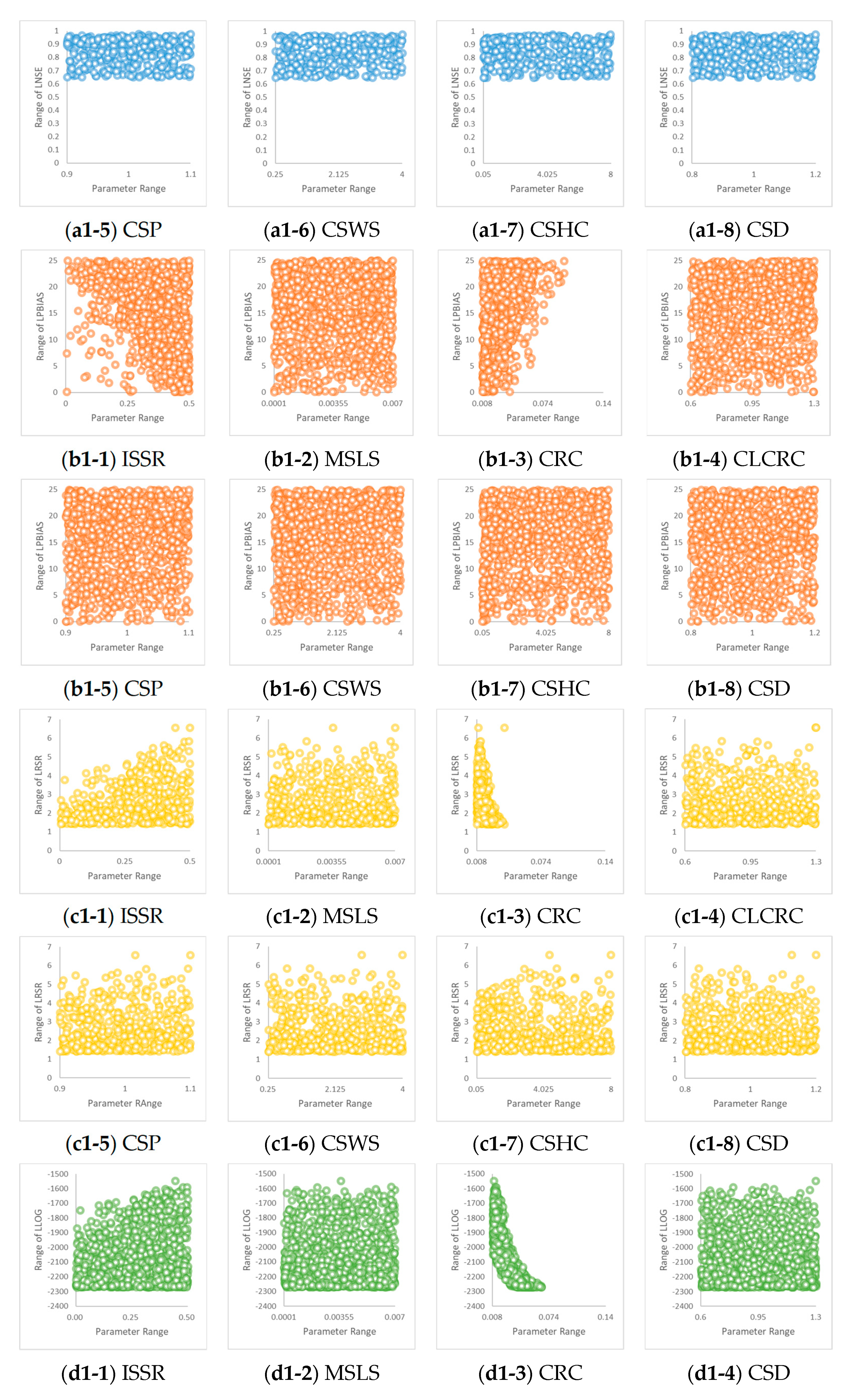
Figure 5 presents the result of dot plot analysis on Event 1. LNSE was represented by a blue circle, and CRC was sensitive. LPBIAS was represented by an orange circle, and ISSR and CRC were sensitive. LRSR was represented by a yellow circle, and ISSR and CRC were sensitive. LLOG was represented by a green circle, and ISSR and CRC were sensitive. In particular, CRC exhibited a tendency of satisfaction within a specific range for all likelihood estimators. Thus, the sensitivity of each parameter varied in the parameter sensitivity analysis for each likelihood, showing that the sensitive range of each parameter type differed.
3.1.2. Event 2 Dotty Plot
Figure 6 shows the results of the dot plot analysis on Event 2. LNSE was indicated by a blue circle, and CRC and CSHC were sensitive. LPBIAS was indicated by an orange circle, and all parameters exhibited a uniform distribution. LRSR was indicated by a yellow circle, and ISSR, CRC, and CSHC were sensitive. LLOG was indicated by a green circle, and ISSR, CRC, and CSHC were sensitive. In particular, CRC exhibited a tendency of satisfaction within a specific range.
The sensitive parameters revealed by the dot plot analysis of the two rainfall events were determined to be ISSR, CRC, and CSHC. In particular, CRC exhibited a tendency of satisfaction within a specific range. The behavioral model of the selected parameters is skewed to one side, meaning that the parameters are sensitive to the GRM result. In contrast, the likelihood for the remaining four parameters, including MSLS, is evenly distributed in the range of the given parameter. This phenomenon could be attributed to the random generation of the parameters in a uniform distribution, as well as their insignificant effect on the GRM results.
3.2. Posterior Distribution of GRM Parameters
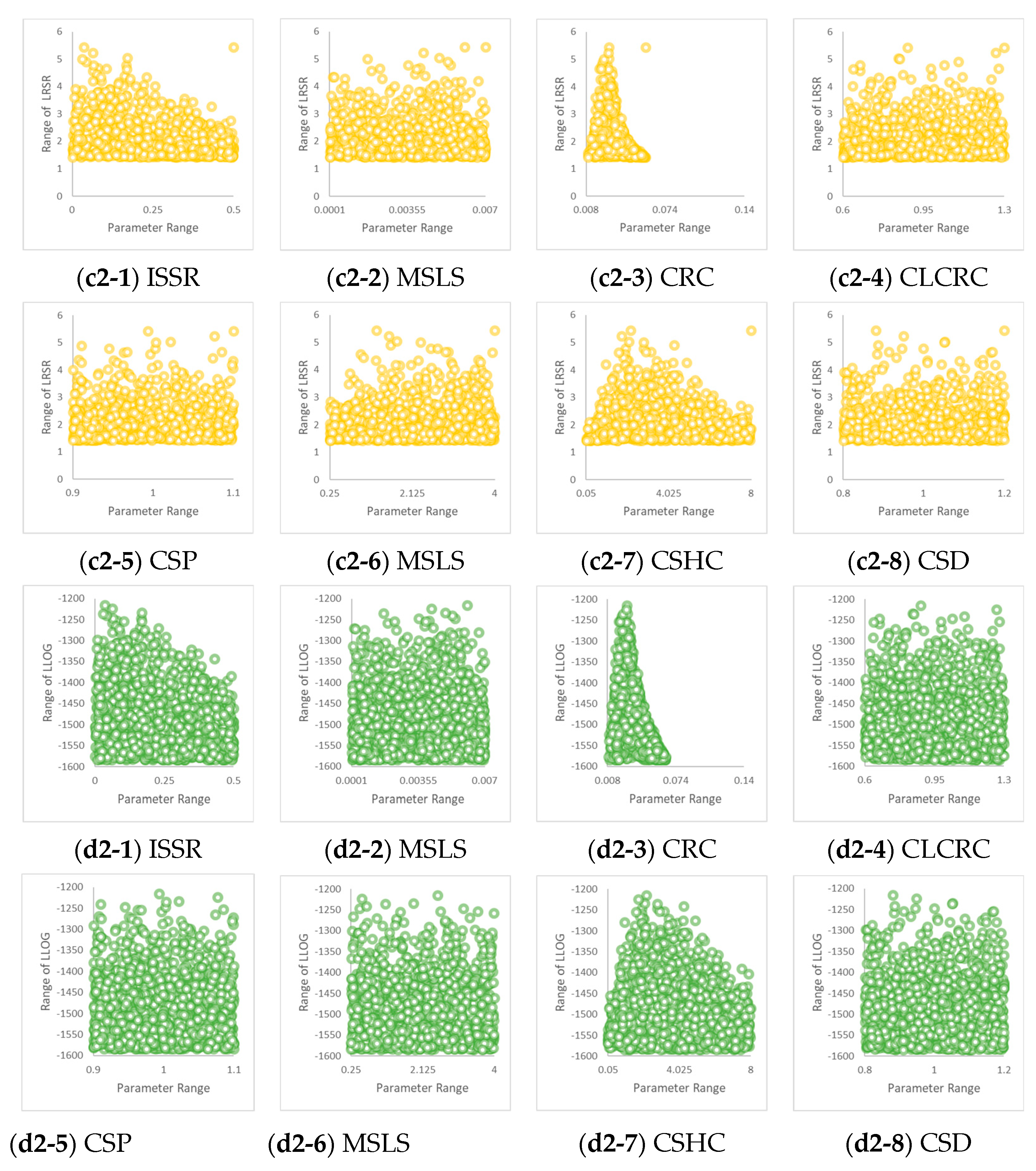
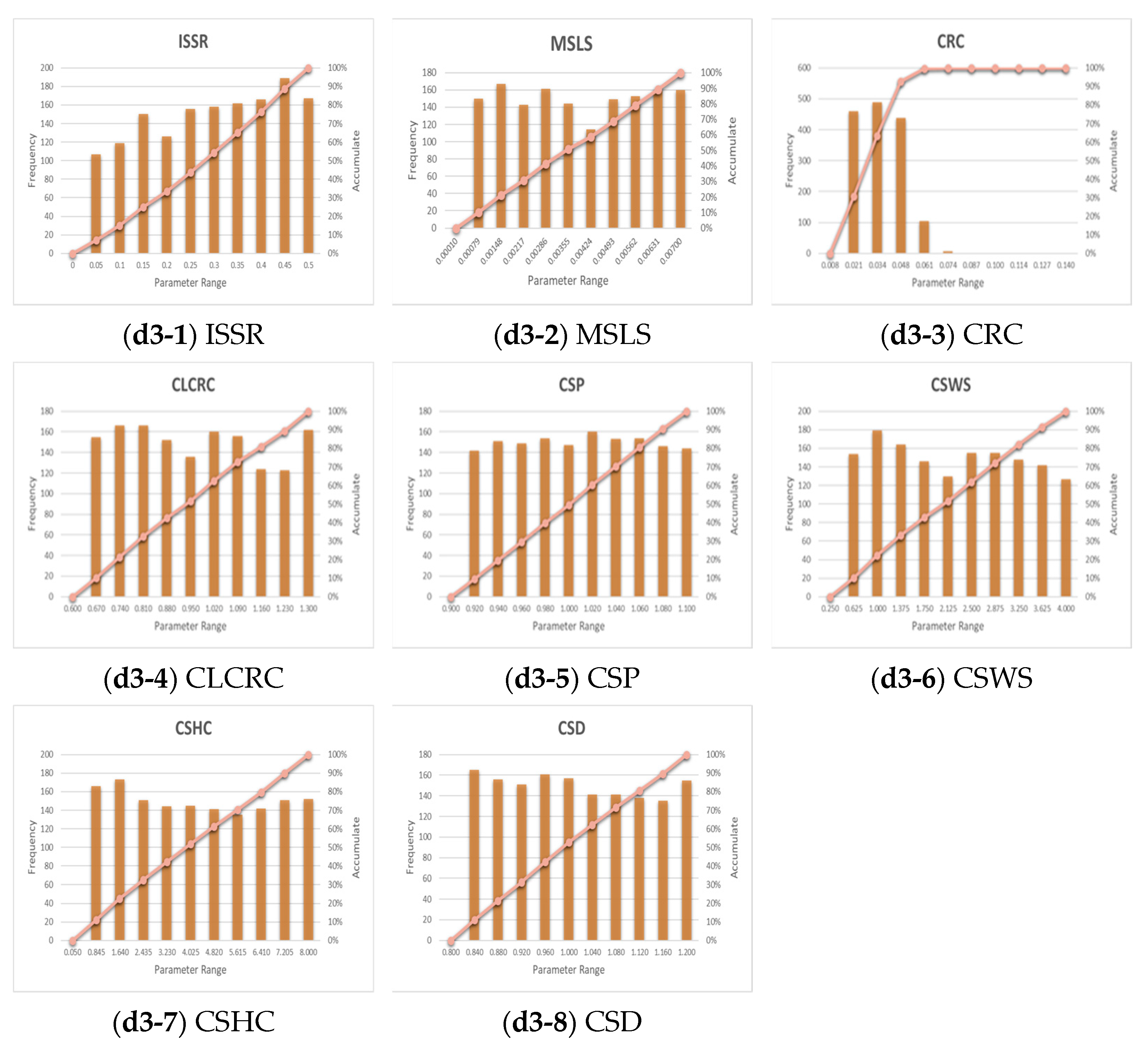
The posterior distributions of the GRM parameters for each likelihood were visualized as histograms (Figure 6). The posterior distribution of a parameter is obtained by a product of likelihood and prior distribution. Since the prior distribution is a uniform distribution, the posterior distribution can be considered to have the same shape as the likelihood. Thus, this study utilized the CDF, rather than the PDF, according to the value of each parameter for the histograms to enhance understanding. In addition, to present the results by likelihood, LNSE, LPBIAS, LRSR, and LLOG were represented in blue, red, green, and brown, respectively.
3.2.1. Event 1 Parameter Sensitivity
According to Figure 7, LNSE showed the better results. As the value of ISSR increased, CRC indicated good results only in a specific range on the left side, and CSHC showed the better results as the value of ISSR decreased. LPBIAS, the second likelihood, became more sensitive as the value of ISSR increased. CRC indicated a tendency of being highly sensitive in a specific range on the left side, and CSHC became sensitive in the range where the value of ISSR was low. LRSR, the third likelihood, became more sensitive as the value of ISSR increased. CRC showed good results only in a specific range on the left side, and CSHC indicated the better results as the value of ISSR decreased. Lastly, LLOG displayed better results as the value of ISSR increased. CRC indicated good results only in a specific range on the left side, and CSHC showed better results in a range where the value of ISSR was relatively low.
3.2.2. Event 2 Parameter Sensitivity
According to Figure 8. LNSE showed better results as the value of ISSR increased; CRC indicated good results only in a specific range on the left side, CSP displayed relatively better results as the value of ISSR decreased, and CSHC indicated good results in a range on the left center. LPBIAS, the second likelihood, showed better results as the value of ISSR decreased, while CRC indicated better results as the value of ISSR increased; CSP showed better results as the value of ISSR became relatively lower, and CSHC indicated good results in a range on the left center. LRSR, the third likelihood, exhibited better results as the value of ISSR decreased; CRC indicated good results only in a specific range, CSP showed better results as the value of ISS became relatively lower, and CSHC indicated good results in a range on the left center. Lastly, LLOG displayed better results as the value of ISSR decreased; CRC showed good results only in a specific range, CSP showed better results as the value of ISS became relatively lower, and CSHC indicated good results in a range on the left center.
As shown in the point distribution, regarding the posterior distribution for each likelihood, the lateral tidal coefficient had a concentrated probability in a certain range. The probability for hydraulic conductivity and soil wetting front became higher as their values decreased, as did the probability for initial saturation profile. In contrast, the posterior distribution of the remaining four parameters, which are insensitive, showed a uniform distribution shape similar to that of the prior distribution. This study found similar posterior distributions according to the four likelihood estimators. However, some parameters showed a similar trend of LPBIAS, whereas some parameters indicated different ranges of CRC parameters.
3.3. Quantied Uncertainty in the GRM Model
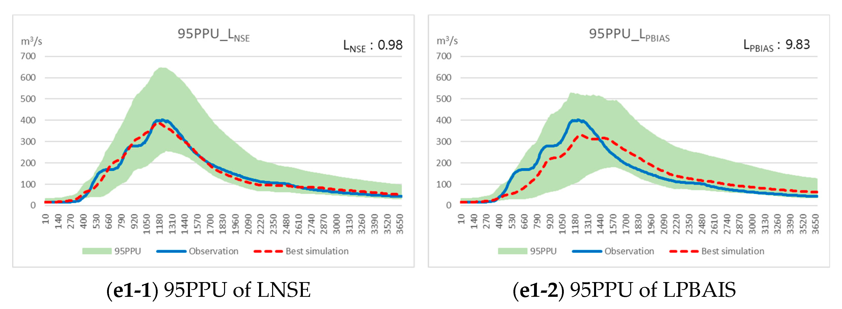
This study applied formal likelihood (NSE, RSR, PBIAS) and informal likelihood (log−normal) to evaluate the uncertainty of the GRM. Despite the application of different types of likelihood, there was a similar trend in the uncertainty range of the runoff by the GRM between LNSE and LRSR in the case of Event 1 (Figure 9). Moreover, there was a similar trend in the uncertainty range of the runoff by the GRM among the likelihood in the case of Event 2, except for LPBIAS (Figure 10). Figure 9 and Figure 10 show the uncertainty range of the GRM depending on likelihood. Here, the uncertainty range refers to 95PPU (percent prediction uncertainty), which is the difference between the cumulative distributions of 2.5% and 97.5%.
3.3.1. Event 1 95PPU
Based on the analysis results for Event 1, the number of behavioral models satisfying the threshold for each likelihood was determined to be 406, 1136, and 533 for LNSE, LPBIAS, and LRSR, respectively. Furthermore, the results satisfying the threshold for likelihood were utilized to construct a CDF of each hourly flow rate in conducting 95PPU analysis.
Regarding the 95PPU analysis results for each likelihood in the case of Event 1, there was a significant similarity in shape and range between the 95PPU ranges of LNSE and LRSR, whereas LPBIAS and LLOG showed different uncertainty distributions. In particular, the uncertainty distribution curves in the rising interval are located in the middle of the range of the observed values in the case of LNSE and LRSR, whereas the uncertainty distribution curves are located in the upper part of the uncertainty range in the case of LPBIAS and LLOG. This result suggests that the simulated flow rate in the rising interval may be slightly underestimated when LPBIAS and LLOLG are used as GoF indices. In contrast, the observed values are located in the lower part of uncertainty range for all likelihood values in the descending interval. These results suggest that the simulated flow rate for all likelihood values can be overestimated in the descending interval. Moreover, these results suggest that a high value of one likelihood with a certain combination of parameters does not necessarily lead to the high values of other likelihood estimates. In this regard, the combination of parameters with the highest LNSE value does not result in that the high values of LPBIAS, LRSR, and LLOG.
In the uncertainty analysis using LPBIAS, the simulated flow rate was determined to be highly similar to the observed flow rate. In addition, 95PPU included the observed flow rate. In this case, the highest value of the calculated LNSE was found to be 0.98. However, when different likelihood values were calculated with a combination of parameters with an LNSE of 0.98, the likelihood values were determined as follows: LBIAS: 5.95, LRSR: 6.56, and LLOG: −1546. The 95PPU for the uncertainty constructed with LNSE is represented by the green area, as shown in Figure 9, and the flow rate simulated with a combination of parameters with an LNSE of 0.98 is indicated by a red dotted line, as shown in Figure 9, which corresponds to the optimal value at 95PPU.
3.3.2. Event 2 95PPU
Based on the analysis results for Event 2, the number of behavioral models satisfying the threshold for each likelihood was determined to be 752, 3721, and 1007 for LNSE, LPBIAS, and LRSR, respectively. Furthermore, the results satisfying the threshold for likelihood were utilized to construct a CDF of each hourly flow rate in conducting 95PPU analysis.
Regarding the 95PPU analysis results for each likelihood in the case of Event 2, there was a significant similarity in shape and range between the 95PPU ranges of LNSE, LRSR, and LLOG, whereas LPBIAS showed different uncertainty distributions. In particular, the uncertainty distribution curves in the rising interval were located in the middle of the range of the observed values in the case of LNSE and LRSR, whereas the uncertainty distribution curves were located in the upper part of the uncertainty range in the case of LPBIAS. This result suggests that the simulated flow rate in the rising interval may be slightly underestimated when LPBIAS is used as the GoF index. In contrast, the observed values were located in the lower part of the uncertainty range for all likelihood estimators in the descending interval. These results suggest that the simulated flow rate for all likelihood models can be overestimated in the descending interval.
In the uncertainty analysis using LNSE, the simulated flow rate was determined to be highly similar than the observed flow rate. In addition, 95PPU included the observed flow rate. In this case, the highest value of the calculated LNSE was found to be 0.97. However, when different likelihood estimates were calculated with a combination of parameters with an LNSE of 0.97, the values were determined as follows: LBIAS: 67.25, LRSR: 5.43, and LLOG: −1215. The 95PPU for the uncertainty constructed with LNSE is represented in the green area, as shown in Figure 10, and the flow rate simulated with a combination of parameters with an LNSE of 0.97 is indicated by a red dotted line, as shown in Figure 10, which corresponds to the optimal value at 95PPU.
4. Discussion
This study used the GRM model developed in South Korea, rather than conventional models, to apply a rainfall−runoff model to flood prediction and model validation, quantify the uncertainty of the domestic model for rainfall−runoff analysis, and evaluate its applicability and reliability. Log−normal formal likelihood was available for this study because a statistical structure for simulation error was established by performing flood case analysis for the same target watershed. Moreover, the uncertainty of parameters in the GRM model was quantified by utilizing informal likelihood estimators such as NSE, RSR, and PBIAS. However, this selection of likelihood estimators resulted in the calculation of different uncertainty ranges, which suggests the intervention of subjective factors. The GoF of models using NSE, RSR, and PBIAS has been discussed in copious literature. In particular, Moriasi [34] stated the reliability of the hydrologic model by classifying thresholds for various GoF indicators, including NSE, and proposed the NSE value of 0.5 or higher as the level satisfying the GoF of the model. However, there has been no previous study on the log−normal threshold for the reliability of the GRM model based on log−normal likelihood. Since the range of log−normal likelihood is from 0 to −∞, it is difficult to select a threshold. Considering this issue, in the case of informal likelihood, this study analyzed the GRM uncertainty for log−normal likelihood by selecting an upper 30% value based on the high likelihood value, as in the method proposed by Beven [36,38]. In this study, there were similar results regarding the distribution of parameters by the behavioral model selected by the threshold for both formal and informal likelihood. However, there is debate that different outcomes can be calculated according to subjective selection of likelihood and threshold [39,40]. This study has revealed the difference between the point distribution and the posterior distribution for each parameter. Since the prior distribution is uniform, if the posterior distribution is not uniform and is distorted, the parameter can be considered sensitive to the simulation results of the GRM model in this distorted portion. In addition, if the posterior distribution of the parameter is utilized to adjust the range of its prior distribution and the uncertainty analysis is repeated, the uncertainty range of a more robust GRM can be specified. Furthermore, rainfall−runoff analysis using commercial models has low financial accessibility, while models developed outside Korea may exhibit low utility due to data that do not fit domestic circumstances. In this respect, the GRM model, which has been domestically developed as open source, provides good accessibility and usability for analyzing domestic rainfall runoff. If users upgrade the GRM model and closely share related information with other users, this model will greatly contribute to the establishment of various disaster prevention plans and policies, such as those involving flood analysis, hydrologic curve analysis, and flood forecasting.
5. Conclusions
This study identified the effect of GRM parameters on simulated rainfall−runoff results for the Cheongmicheon Watershed, and quantified (95PPU) the uncertainty of the runoff values, which are the simulated results of the GRM, for the observed values. In particular, because in the uncertainty analysis using GLUE the uncertainty range can vary depending on the effect of the likelihood function, this study used formal and informal likelihood to calculate the uncertainty of the parameters, and conducted a comparative analysis. All eight parameters constituting the GRM model were selected for both formal and informal likelihood. This study revealed that the commonly sensitive parameters among the GRM parameters were CRC and CSHC, thereby identifying the ranges showing good results. Although the prior distributions of parameters were uniform, behavioral models were determined with the threshold values of the upper 30% for formal likelihood, and with the cases where the NSE value was 0.65 or higher, PBIAS < |25|, and RSR < 0.7, as proposed by Moriasi [34]. Behavioral models generated from both formal and in formal likelihood showed a skewed distribution to the left (CRC), or the left center (CSHC) in the posterior distribution. For LNSE, LRSR, and LLOG, there was a skewed distribution to the left in both CRC and hydraulic conductivity, while for PBAIS, there was a skewed distribution to the right (CRC), or to the left (CSHC). Uncertainties were quantified by using three types of informal likelihood—LNSE, LPBIAS, and LRSR—and formal likelihood—LLOG. Despite the difference in sensitivity across the parameters for each likelihood, there was a similar distribution in the likelihood values for the ranges according to the LNSE, LRSR, and LLOG parameters. In addition, the uncertainty range revealed through the 95PPU analysis indicated a similar shape. In contrast, the distribution of the behavioral model in LPBIAS differed from that of other likelihoods, suggesting that the observed value was not included in 95PPU. The change of parameters for each rainfall pattern varied, showing a different runoff depending on circumstances. Furthermore, based on the results of evaluation using LNSE, LRSR, LPBIAS, and LLOG, it was confirmed that uncertainty for each parameter can be differently calculated depending on likelihood. According to the results from the 95PPU analysis under the likelihood conditions given in this study, LNSE and LRSR likelihood, rather than LPBIAS, estimators were determined to be appropriate for evaluation via runoff model. In addition, if the range of LLOG can be defined, evaluation of uncertainty using formal likelihood becomes appropriate. However, these results suggest that it is important to secure consistency in the uncertainty range by applying various likelihood estimates and thresholds.
Author Contributions
Conceptualization, Y.S. and Y.J.; methodology, Y.S.; software, Y.S.; validation, Y.S.; formal analysis, Y.S.; investigation, Y.S., Y.J. and C.-K.C.; resources, Y.S., Y.J. and C.-K.C.; data curation, Y.S., Y.J. and C.-K.C.; writing—original draft preparation, Y.S.; writing—review and editing, Y.S., Y.J. and C.-K.C.; visualization, Y.S.; supervision, Y.J.; project administration, Y.J.; funding acquisition, Y.J. All authors have read and agreed to the published version of the manuscript.
Funding
This work was supported by Korea Environment Industry and Technology Institute (KEITI) through Water Management Research Program, funded by Korea Ministry of Environment (MOE) (139266).
Institutional Review Board Statement
Not applicable.
Informed Consent Statement
Not applicable.
Data Availability Statement
Data is available on request.
Acknowledgments
Jung, Y. acknowledged the financial support of the Department of Advanced Science and Technology Convergence at Kyungpook National University. The authors acknowledge the efforts of the anonymous reviewers that worked on the manuscript.
Conflicts of Interest
The authors declare no conflict of interest.
References
- Tayfur, G.; Singh, V.P. ANN and Fuzzy Logic Models for Simulating Event−Based Rainfall−Runoff. J. Hydraul. Eng. 2006, 132, 1321–1330. [Google Scholar] [CrossRef] [Green Version]
- Tramblay, Y.; Bouvier, C.; Martin, C.; Didon−Lescot, J.F.; Todorovik, D.; Domergue, J.M. Assessment of initial soil moisture conditions for event−based rainfall–runoff modelling. J. Hydrol. 2010, 387, 176–187. [Google Scholar] [CrossRef]
- Talei, A.; Chua, L.H. Influence of lag time on event−based rainfall–runoff modeling using the data driven approach. J. Hydrol. 2012, 438, 223–233. [Google Scholar] [CrossRef]
- Chang, T.K.; Talei, A.; Alaghmand, S.; Ooi, M.P.L. Choice of rainfall inputs for event−based rainfall−runoff modeling in a catchment with multiple rainfall stations using data−driven techniques. J. Hydrol. 2017, 545, 100–108. [Google Scholar] [CrossRef]
- Reshma, T.; Venkata Reddy, K.; Pratap, D.; Agilan, V. Parameters optimization using Fuzzy rule based multi−objective genetic algorithm for an event based rainfall−runoff model. Water Resour. Manag. 2018, 32, 1501–1516. [Google Scholar] [CrossRef]
- Beven, K.; Binley, A. The future of distributed models: Model calibration and uncertainty prediction. Hydrol. Process. 1992, 6, 279–298. [Google Scholar] [CrossRef]
- Geza, M.; McCray, J.E. Effects of soil data resolution on SWAT model stream flow and water quality predictions. J. Environ. Manag. 2008, 88, 393–406. [Google Scholar] [CrossRef]
- Shen, Z.Y.; Hong, Q.; Yu, H.; Niu, J.F. Parameter uncertainty analysis of non−point source pollution from different land use types. Sci. Total Environ. 2010, 408, 1971–1978. [Google Scholar] [CrossRef]
- Zehe, E.; Becker, R.; Bárdossy, A.; Plate, E. Uncertainty of simulated catchment runoff response in the presence of threshold processes: Role of initial soil moisture and precipitation. J. Hydrol. 2005, 315, 183–202. [Google Scholar] [CrossRef]
- Mohamadi, M.A.; Kavian, A. Effects of rainfall patterns on runoff and soil erosion in field plots. J. Soil Water Conserv. 2015, 3, 273–281. [Google Scholar] [CrossRef] [Green Version]
- Tang, X.; Zhang, J.; Wang, G.; Jin, J.; Liu, C.; Liu, Y.; He, R.; Bao, Z. Uncertainty Analysis of SWAT Modeling in the Lancang River Basin Using Four Different Algorithms. Water 2021, 13, 341. [Google Scholar] [CrossRef]
- Ebtehaj, M.; Moradkhani, H.; Gupta, H.V. Improving robustness of hydrologic parameter estimation by the use of moving block bootstrap resampling. Water Resour. Res. 2010, 46, 7. [Google Scholar] [CrossRef]
- Chaubey, I.; Haan, C.T.; Grunwald, S.; Salisbury, J.M. Uncertainty in the model parameters due to spatial variability of rainfall. J. Hydrol. 1999, 220, 48–61. [Google Scholar] [CrossRef] [Green Version]
- Binley, A.M.; Beven, K.J.; Calver, A.; Watts, L.G. Changing responses in hydrology: Assessing the uncertainty in physically based model predictions. Water Resour. Res. 1991, 27, 1253–1261. [Google Scholar] [CrossRef]
- Melching, C.S. An improved first−order reliability approach for assessing uncertainties in hydrologic modeling. J. Hydrol. 1992, 132, 157–177. [Google Scholar] [CrossRef]
- Hossain, F.; Anagnostou, E.N.; Bagtzoglou, A.C. On Latin Hypercube sampling for efficient uncertainty estimation of satellite rainfall observations in flood prediction. Comput. Geosci. 2006, 32, 776–792. [Google Scholar] [CrossRef]
- Durbin, J.; Koopman, S.J. Time Series Analysis by State Space Methods; OUP Oxford: Oxford, UK, 2012; Volume 38. [Google Scholar]
- Vrugt, J.A.; Braak, C.J.F.T.; Gupta, H.V.; Robinson, B.A. Response to comment by Keith Beven on “Equifinality of formal (DREAM) and informal (GLUE) Bayesian approaches in hydrologic modeling?”. Stoch. Environ. Res. Risk Assess. 2009, 23, 1061–1062. [Google Scholar] [CrossRef]
- Dettinger, M.D.; Wilson, J.L. First order analysis of uncertainty in numerical models of groundwater flow part: 1. Mathematical development. Water Resour. Res. 1981, 17, 149–161. [Google Scholar] [CrossRef] [Green Version]
- Townley, L.R.; Wilson, J.L. Computationally efficient algorithms for parameter estimation and uncertainty propagation in numerical models of groundwater flow. Water Resour. Res. 1985, 21, 1851–1860. [Google Scholar] [CrossRef]
- Nourali, M.; Ghahraman, B.; Pourreza−Bilondi, M.; Davary, K. Effect of formal and informal likelihood functions on uncertainty assessment in a single event rainfall−runoff model. J. Hydrol. 2016, 540, 549–564. [Google Scholar] [CrossRef]
- Hu, C.; Xia, J.; She, D.; Song, Z.; Zhang, Y.; Hong, S. A new urban hydrological model considering various land covers for flood simulation. J. Hydrol. 2021, 603, 126833. [Google Scholar] [CrossRef]
- Christensen, S. A synthetic groundwater modelling study of the accuracy of GLUE uncertainty intervals. Hydrol. Res. 2004, 35, 45–59. [Google Scholar] [CrossRef]
- Montanari, A. Large sample behaviors of the generalized likelihood uncertainty estimation (GLUE) in assessing the uncertainty of rainfall−runoff simulations. Water Resour. Res. 2005, 41, 8. [Google Scholar] [CrossRef]
- McMillan, H.; Clark, M. Rainfall−runoff model calibration using informal likelihood measures within a Markov chain Monte Carlo sampling scheme. Water Resour. Res. 2009, 45, 4. [Google Scholar] [CrossRef]
- Choi, Y.S.; Choi, C.K.; Kim, H.S.; Kim, K.T.; Kim, S. Multi−site calibration using a grid−based event rainfallrunoff model: A case study of the upstream areas of the Nakdong River basin in Korea. Hydrol. Process. 2015, 29, 2089–2099. [Google Scholar] [CrossRef]
- Shin, M.J.; Choi, Y.S. Sensitivity analysis to investigate the reliability of the grid−based rainfall−runoff model. Water 2018, 10, 1839. [Google Scholar] [CrossRef] [Green Version]
- Hornberger, G.M.; Spear, R.C. Approach to the preliminary analysis of environmental systems. J. Environ. Mgmt. 1981, 12, 7–18. [Google Scholar]
- Young, P. The Validity and Credibility of Models for Badly Defined Systems. In Uncertainty and Forecasting of Water Quality; Beck, M.B., Straten, G.V., Eds.; Springer: Berlin/Heidelberg, Germany, 1983; pp. 69–98. [Google Scholar]
- Jin, X.; Xu, C.Y.; Zhang, Q.; Singh, V.P. Parameter and modeling uncertainty simulated by GLUE and a formal Bayesian method for a conceptual hydrological model. J. Hydrol. 2010, 383, 147–155. [Google Scholar] [CrossRef]
- Blasone, R.S.; Madsen, H.; Rosbjerg, D. Uncertainty assessment of integrated distributed hydrological models using GLUE with Markov chain Monte Carlo sampling. J. Hydrol. 2008, 353, 18–32. [Google Scholar] [CrossRef] [Green Version]
- Nash, J.E.; Sutcliffe, J.V. River flow forecasting through conceptual models part I—A discussion of principles. J. Hydrol. 1970, 10, 282–290. [Google Scholar] [CrossRef]
- Gupta, H.V.; Sorooshian, S.; Yapo, P.O. Status of automatic calibration for hydrologic models: Comparison with multilevel expert calibration. J. Hydrol. Eng. 1999, 4, 135–143. [Google Scholar] [CrossRef]
- Moriasi, D.N.; Arnold, J.G.; Van Liew, M.W.; Bingner, R.L.; Harmel, R.D.; Veith, T.L. Model evaluation guidelines for systematic quantification of accuracy in watershed simulations. Trans. ASABE 2007, 50, 885–900. [Google Scholar] [CrossRef]
- Legates, D.R.; McCabe, G.J., Jr. Evaluating the use of “goodness−of−fit” measures in hydrologic and hydroclimatic model validation. Water Resour. Res. 1999, 35, 233–241. [Google Scholar] [CrossRef]
- Beven, K. Environmental Modelling: An Uncertain Future? Routledge: New York, NY, USA, 2009. [Google Scholar]
- Ajmal, M.; Kim, T.W. Quantifying excess stormwater using SCS−CN–based rainfall runoff models and different curve number determination methods. J. Irrig Drain. Eng. 2015, 141, 04014058. [Google Scholar] [CrossRef]
- Jung, Y.; Merwade, V. Uncertainty quantification in flood inundation mapping using generalized likelihood uncertainty estimate and sensitivity analysis. J. Hydrol. Eng. 2012, 17, 507–520. [Google Scholar] [CrossRef]
- Jung, Y.; Merwade, V.; Kim, S.; Kang, N.; Kim, Y.; Lee, K.; Kim, G.; Kim, H.S. Sensitivity of subjective decisions in the GLUE methodology for quantifying the uncertainty in the flood inundation map for Seymour reach in Indiana, USA. Water 2014, 6, 2104–2126. [Google Scholar] [CrossRef] [Green Version]
- Zhang, Y.; Liu, H.H.; Houseworth, J. Modified generalized likelihood uncertainty estimation (GLUE) methodology for considering the subjectivity of likelihood measure selection. J. Hydrol. Eng. 2011, 16, 558–561. [Google Scholar] [CrossRef]
Figure 1.
Hydrologic network of Study area.

Figure 2.
Schematic of the grid-based rainfall-runoff model (GRM).

Figure 3.
Spatial data of study site (a) Digital Elevation Model; (b) Land cover map; Attributes 1 to 7 represent city/dry area, agricultural area, forest area, meadow, wetland, bare land, and water; (c) Land cover map; Attributes 1 to 8 represent silty clay loam, silt loam, sandy loam, sand, clay loam, clay, loamy sand, loam, respectively; (d) Soil depth map; Attributes 1 to 4 represent very shallow, shallow, moderately deeper, deep, respectively.

Figure 4.
GRM parameter uncertainty estimation method.

Figure 5.
Event 1 Dotty plot of behavioral parameters based on formal and informal likelihood. (a1-1–a1-8) LNSE results; (b1-1–b1-8) LPBIAS results; (c1-1–c1-8) LRSR results; (d1-1–d1-8) LLOG results.
Figure 5.
Event 1 Dotty plot of behavioral parameters based on formal and informal likelihood. (a1-1–a1-8) LNSE results; (b1-1–b1-8) LPBIAS results; (c1-1–c1-8) LRSR results; (d1-1–d1-8) LLOG results.


Figure 6.
Event 2 dotty plot of behavioral parameters based on formal and informal likelihood. (a2-1–a2-8) LNSE results; (b2-1–b2-8) LPBIAS results; (c2-1–c2-8) LRSR results; (d2-1–d2-8) LLOG results.
Figure 6.
Event 2 dotty plot of behavioral parameters based on formal and informal likelihood. (a2-1–a2-8) LNSE results; (b2-1–b2-8) LPBIAS results; (c2-1–c2-8) LRSR results; (d2-1–d2-8) LLOG results.


Figure 7.
Event 1 parameter sensitivity (histogram/CDF). (a3-1–a3-8) LNSE results; (b3-1–b3-8) LPBIAS results; (c3-1–c3-8) LRSR results; (d3-1–d3-8) LLOG results.
Figure 7.
Event 1 parameter sensitivity (histogram/CDF). (a3-1–a3-8) LNSE results; (b3-1–b3-8) LPBIAS results; (c3-1–c3-8) LRSR results; (d3-1–d3-8) LLOG results.


Figure 8.
Event 2 parameter sensitivity (histogram/CDF). (a4-1–a4-8) LNSE results; (b4-1–b4-8) LPBIAS results; (c4-1–c4-8) LRSR results; (d4-1–d4-8) LLOG results.
Figure 8.
Event 2 parameter sensitivity (histogram/CDF). (a4-1–a4-8) LNSE results; (b4-1–b4-8) LPBIAS results; (c4-1–c4-8) LRSR results; (d4-1–d4-8) LLOG results.


Figure 9.
Event 1 95PPU. (e1-1) LNSE results; (e1-2) LPBIAS results; (e1-3) LRSR results; (e1-4) LLOG results.
Figure 9.
Event 1 95PPU. (e1-1) LNSE results; (e1-2) LPBIAS results; (e1-3) LRSR results; (e1-4) LLOG results.


Figure 10.
Event 2 95PPU. (e2-1) LNSE results; (e2-2) LPBIAS results; (e2-3) LRSR results; (e2-4) LLOG results.
Figure 10.
Event 2 95PPU. (e2-1) LNSE results; (e2-2) LPBIAS results; (e2-3) LRSR results; (e2-4) LLOG results.


Table 1.
Rainfall Station and Thiessen Weight.
| Rainfall Station Name | Rainfall Station Location | Station Weight (%) | |
|---|---|---|---|
| Latitude | Longitude | ||
| Samjuk | 37°4′36.36″ N | 127°22′7.03″ E | 26.13 |
| Geumdang Elementary School | 37°12′3.45″ N | 127°36′21.74″ E | 17.51 |
| Beopcheon | 37°12′16.31″ N | 127°44′52.87″ E | 15.78 |
| Yeoju Bridge | 37°17′43.27″ N | 127°38′31.92″ E | 14.03 |
| Wonsam | 37°10′6.32″ N | 127°18′15.06″ E | 9.01 |
| Seolseong | 37° 8′45.33″ N | 127°31′17.97″ E | 7.24 |
| Saenggeu | 37° 2′4.37″ N | 127°36′3.93″ E | 4.56 |
| Eumseong | 36°56′13.82″ N | 127°41′32.14″ E | 2.18 |
| Namgok | 37°13′53.30″ N | 127°16′41.07″ E | 1.71 |
| Angseong | 37° 5′11.35″ N | 127°44′43.87″ E | 1.50 |
| Oryu | 36°58′21.40″ N | 127°28′40.99″ E | 0.35 |
Table 2.
Duration of Rainfall Event.
| Num | NAME | Start Date | End Date |
|---|---|---|---|
| 1 | Event 1 | 29 June 2011 (10:00:00) | 1 July 2011 (17:30:00) |
| 2 | Event 2 | 31 July 2017 (3:00:00) | 1 August 2012 (07:30:00) |
Table 3.
GRM Parameters Description and Range.
| Num | Parameters | Description | Range | Change Range | ||
|---|---|---|---|---|---|---|
| Lower | Upper | Lower | Upper | |||
| 1 | IniSaturation (ISSR) | Initial soil saturation ratio | 0 | 1 | 0 | 0.5 |
| 2 | MinSlopeOF (MSLS) | Minimum slope of land surface | 0.0001 | 0.01 | 0.0001 | 0.007 |
| 3 | ChRoughness (CRC) | Channel roughness coefficient | 0.008 | 0.2 | 0.008 | 0.14 |
| 4 | CalCoefLCRoughness (CLCRC) | Correction factor for land cover roughness coefficient | 0.6 | 1.3 | 0.6 | 1.3 |
| 5 | CalCoefSoilDepth (CSD) | Correction factor for soil depth | 0.8 | 1.2 | 0.9 | 1.1 |
| 6 | CalCoefPorosity (CSP) | Correction factor for soil porosity | 0.9 | 1.1 | 0.25 | 4 |
| 7 | CalCoefWFSuctionHead (CSWS) | Correction factor for soil wetting front suction head | 0.25 | 4 | 0.05 | 8 |
| 8 | CalCoefHydraulicK (CSHC) | Correction factor for soil hydraulic conductivity | 0.05 | 20 | 0.8 | 1.2 |
Publisher’s Note: MDPI stays neutral with regard to jurisdictional claims in published maps and institutional affiliations. |
© 2022 by the authors. Licensee MDPI, Basel, Switzerland. This article is an open access article distributed under the terms and conditions of the Creative Commons Attribution (CC BY) license (https://creativecommons.org/licenses/by/4.0/).
Share and Cite
MDPI and ACS Style
Seong, Y.; Choi, C.-K.; Jung, Y. Assessment of Uncertainty in Grid-Based Rainfall-Runoff Model Based on Formal and Informal Likelihood Measures. Water 2022, 14, 2210. https://doi.org/10.3390/w14142210
AMA Style
Seong Y, Choi C-K, Jung Y. Assessment of Uncertainty in Grid-Based Rainfall-Runoff Model Based on Formal and Informal Likelihood Measures. Water. 2022; 14(14):2210. https://doi.org/10.3390/w14142210
Chicago/Turabian StyleSeong, Yeonjeong, Cheon-Kyu Choi, and Younghun Jung. 2022. "Assessment of Uncertainty in Grid-Based Rainfall-Runoff Model Based on Formal and Informal Likelihood Measures" Water 14, no. 14: 2210. https://doi.org/10.3390/w14142210
Note that from the first issue of 2016, this journal uses article numbers instead of page numbers. See further details here.