
On the Use of Gridded Data Products for Trend Assessment and Aridity Classification in a Mediterranean Context: The Case of the Apulia Region


Department of Civil, Environmental and Architectural Engineering, University of L’Aquila, Via G. Gronchi, 18, 67100 L’Aquila, Italy
*
Author to whom correspondence should be addressed.
Water 2022, 14(14), 2203; https://doi.org/10.3390/w14142203
Submission received: 19 May 2022
/
Revised: 4 July 2022
/
Accepted: 11 July 2022
/
Published: 12 July 2022
(This article belongs to the Special Issue Evaluation of Reanalysis Data in Meteorological and Climatological Applications: Spatial and Temporal Considerations)
Abstract
:Large-scale gridded climatic data can be useful for the assessment of climate variability and change as a basis for understanding and monitoring natural hazards, as well as for determining appropriate coping strategies. However, an evaluation of the accuracy of these data products against local observational measurements over the different regions of the globe is always required, as these large-scale data may be affected by systematic errors, which can affect the results of downstream applications. Therefore, this study was carried out to evaluate the performances of two long-term gridded datasets in reproducing station-based precipitation and temperature data over the Apulia region (southern Italy) for the period 1956–2019, with a particular focus on the effect of using the different data sources on the results of trend analyses and aridity classification. The results revealed that the considered gridded data products allow only general indications on the spatial and temporal behavior of climatic variables over the Apulia region, especially in regard to precipitation data.
Keywords:
precipitation; temperature; station data; gridded data; E-OBS; CRU; climate; trend; aridity; Apulia region1. Introduction
On a global scale, extreme weather events, causing major adverse impacts on populations, economies and the environment, have been observed becoming more frequent in the last decades because of climate change [1]. In this context of changing climate, the understanding and monitoring of the variability of climatic parameters are crucial for identifying suitable coping strategies against climate-related risks [2,3]. While in situ station data can provide a clear picture of the climate state and its trend in a region of interest, the spatial coverage of dense observation networks over the globe is still highly uneven [4]. To overcome this problem, several global and regional climatic gridded datasets, derived through interpolation of station data, have been released over the years (e.g., [5,6]). These products provide long-term climatic information for large areas, thus making them suitable to be used for applications at any spatial scale. However, in spite of rigorous protocols for their production, these datasets inherently bring potential inaccuracies and errors that may significantly affect the results of downstream applications [7,8,9,10,11,12].
In particular, larger errors are especially expected in regions characterized by complex topographic and/or climatic features as a consequence of the smoothing effect behind the interpolation methods on which gridded data are based [13,14,15,16,17]. In this regard, the Mediterranean region, often referred to as a hotspot for climate change [18], can be considered as a pivotal example because of its transitional position between tropical and temperate climates and its complex orography. Several studies have analyzed recent trends in the main climatic variables for the Mediterranean, identifying a significant warming all over the basin and a weak, although not spatially uniform, decreasing trend in total precipitation (e.g., [19,20,21,22]). The study carried out by Kostopoulou et al. [23] for the eastern Mediterranean region revealed the ability of the E-OBS [5] gridded dataset to satisfactorily reproduce temperature data registered in most of the 54 considered meteorological stations, although with some evident deviations at higher elevations, while a poorer accuracy was found for precipitation data. These general tendencies have been also confirmed and emphasized by studies carried out at smaller spatial scales, relying on more dense observational networks, as shown for instance in Turco et al. [24], Dumitrescu and Birsan [25] and Curci et al. [16].
In this heterogeneous context, it is therefore critical to evaluate the reliability of gridded data products in reproducing local climatic features captured at point meteorological stations, especially when used for performing impact assessments of climate change or deriving conclusions on climate variability. Consequently, more intercomparisons of different data sources in regions with diverse climatology and topography would be beneficial to obtain more insights into the global view of the accuracy and uncertainties related to the use of gridded data.
The present study was then carried out to investigate the different outcomes, in terms of trend assessment and aridity classification, resulting from the analysis of long-term temperature and precipitation observations registered at gauging sites or derived from large-scale gridded datasets. The selected study area is the Apulia region (located in the eastern part of the Mediterranean basin), one of the most climate-vulnerable areas in Italy, challenged by warming, water scarcity and intensive agricultural activities [26]. At the same time, the existence of a robust dense temperature and precipitation gauging network makes it suitable for an intercomparison study aimed at assessing the reliability of large-scale gridded data; such analysis has not already been performed in any of the previous investigations carried out for the region, which were instead aimed at analyzing the impacts of climatic variability on groundwater, agriculture, landslide occurrence and possible desertification [26,27,28,29,30].
The paper is organized as follows: the datasets and the methodology for the intercomparison analysis on the use of the different data sources in terms of trend detection and aridity classification are described in Section 2; Section 3 presents the results of the comparisons and the corresponding discussion, followed by concluding remarks in Section 4.
2. Materials and Methods
2.1. Study Area and Station Data
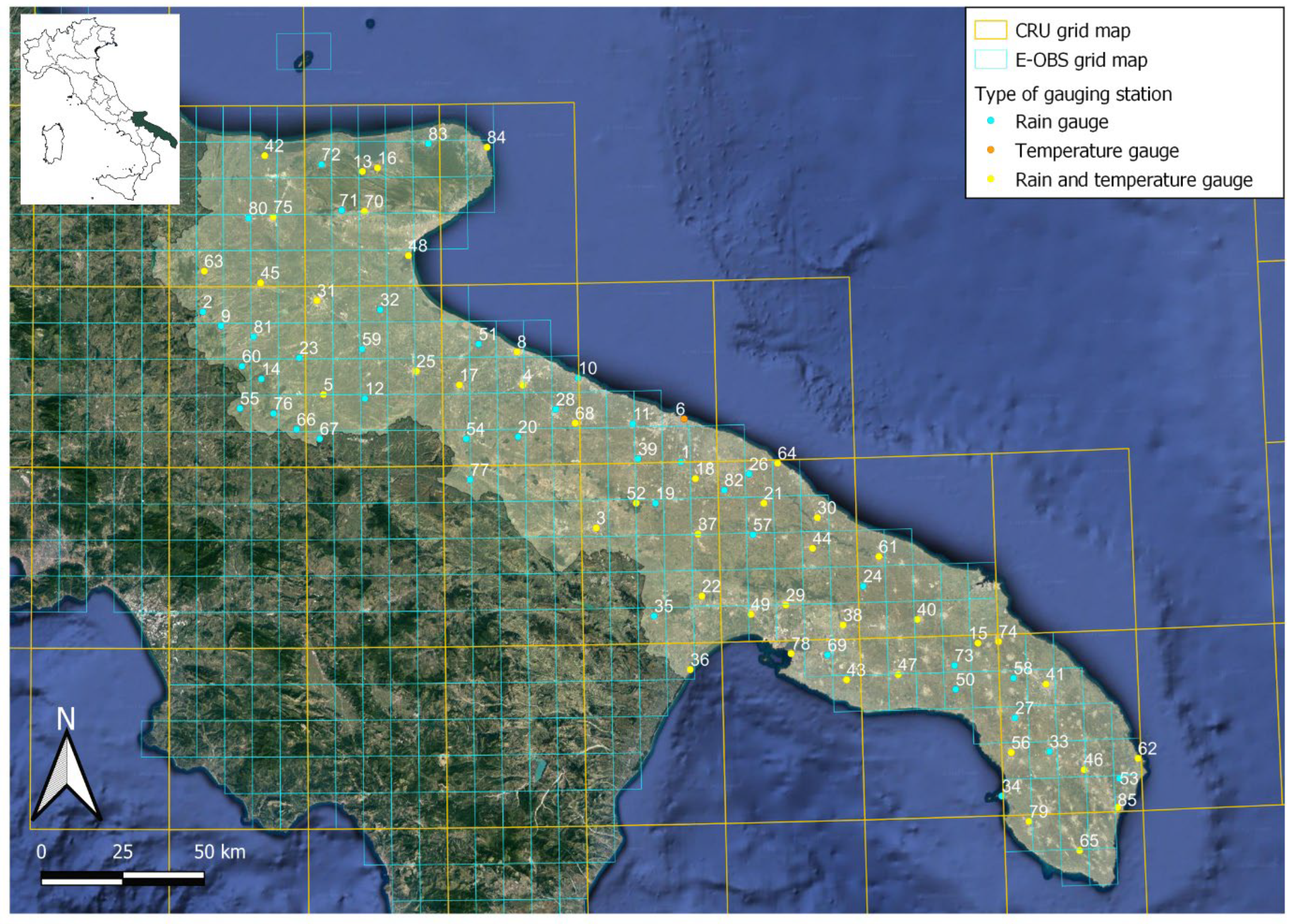
The Apulia region (Figure 1) extends over an area of approximately 20,000 km2 in southern Italy, characterized by a mostly flat topography, with more than 50% of the territory located below 300 m a.s.l. and only a small portion of it (<2%, in the northern part of the region) exceeding 600 m a.s.l.
The climate is typically Mediterranean, with hot, dry and sunny summers and mild and rainy winters, receiving more than 60% of total annual precipitation. The mean annual temperature ranges between 12 °C and 17 °C, with a mean summer temperature of approximately 24 °C. Although dominated by a Mediterranean macroclimate, the morphology of the region determines the occurrence of many local microclimates, with a strong influence of winds, especially over the Adriatic coastal areas.
The station data used in this study as a comparison means for gridded data products derive from a dense observation network managed by the “Centro Funzionale Decentrato della Protezione Civile della Regione Puglia”. The originally available precipitation dataset for the region consisted of monthly rainfall measured at about 140 meteorological stations, while temperature data included registrations for monthly maximum, minimum and mean temperatures at about 100 gauging stations. Preliminary standard quality control procedures (World Meteorological Organization [31]) were applied to the time series to identify nonphysical values (e.g., abnormally high/low temperature, minimum temperature higher than maximum temperature, repeated values, misprints and abrupt jumps) and outliers through comparison with neighboring correlated stations. This study focused on the period 1956–2019 to guarantee a homogenous spatial density of stations over the region and to reduce the number of missing records in the time series. In detail, the final dataset included only those stations having less than five consecutive years of missing data and being characterized by a limited overall percentage of missing annual records, which was set at 10% and 17% for precipitation and temperature measurements, respectively. The final selected dataset at the end of this preprocessing phase then consisted of 84 precipitation and 44 temperature gauging stations (Figure 1 and Table S1). On average, the percentage of missing data in the considered precipitation and temperature time series was, respectively, equal to 2.5% and 8.7%. In this study, it was decided to not apply any filling procedure for the reconstruction of missing values, as well as any homogenization algorithm, in order to avoid the introduction of any bias in the time series used in the comparison with gridded datasets, which themselves can contain inhomogeneities [8,11].
2.2. E-OBS Database
The E-OBS is a database developed at the European level comprising daily values of precipitation and minimum, maximum and mean temperature back to 1950, constructed on a 0.1° regular grid (~11 km × 11 km) through interpolation of the most complete collection of station data over wider Europe [5,32]. All gridded datasets (E-OBS v23.0e, released on March 2021) used in this study are available on the project’s website (www.ecad.eu, accessed on 18 May 2022).
2.3. CRU Database
Similarly to the E-OBS, the CRU dataset, generated by the Climatic Research Unit of the University of East Anglia, provides monthly precipitation as well as minimum, maximum and mean temperature on a 0.5° global grid (~55 × 55 km) back to 1901 [33]. The latest version of the dataset (CRU TS v. 4.05, released on March 2021 and available at https://crudata.uea.ac.uk/cru/data/hrg/, accessed on 18 May 2022), was used in this study.
2.4. Analysis of Temperature, Precipitation and Aridity Indices
Temperature and precipitation station data were compared to the E-OBS and CRU data extracted from the nearest grid cell. The following time series over the common period 1956–2019 were then associated to each station based on available raw monthly data: annual and seasonal precipitation (RR) and annual and seasonal mean temperature I, mean maximum (TX) and minimum (TN) temperature. The different seasons are identified hereinafter by using the following subscripts: spring (spr) (March–April–May) and summer (sum) (June–July–August) for the “warm season” and winter (win) (December–January–February) and autumn (aut) (September–October–November) for the “mild/cold season”. The same time series were derived from the gridded products and associated to the selected sites.
As a first mean for comparison, Taylor diagrams were used to examine how closely gridded precipitation and temperature data resemble in situ registrations. These diagrams can indeed provide a concise overview on the similitude between datasets in terms of three statistics, i.e., the Pearson correlation coefficient, the root-mean-square error and the standard deviation [34].
Then, it was analyzed to what extent the differences in the datasets reflect on the results of trend assessment, in terms of detection of significant/nonsignificant changes and trend magnitude in the climatic variables. To this aim, the nonparametric Mann–Kendall test [35,36] was applied to identify the presence of significant climatic linear trends in the time series of the above-mentioned variables. Trend magnitude was quantified using the Theil–Sen approach [37] and the statistical significance of the trend was assessed at the 5% level. All trend analyses were performed for the individual stations considering the different data sources.
Furthermore, the processed temperature and precipitation data at the selected sites were then used to calculate new annual time series representing aridity indices, calculated based on the three different data sources. For this purpose, we considered two of the most renowned aridity parameters, namely the De Martonne (DMI) and the Pinna combinative (PCI) aridity index [38,39,40], widely used to identify the dry/humid climate conditions of any given region over the globe. The DMI is based on total annual precipitation (P) and mean temperature (), as follows:
The PCI considers also the total precipitation (Pd) and the mean air temperature (Td) of the driest month of the year, in addition to the total annual precipitation and mean temperature, as in the DMI:
The corresponding climatic classification based on the DMI and PCI is provided in Table 1. Then, for the individual sites, a climate type (according to Equations (1) or (2)) was attributed to each year of the time series by considering the three data sources; normalized contingency matrices were computed to evaluate the differences in the classification obtained with the use of the considered datasets.
Similarly to the other climate variables, a trend analysis was also carried out for the calculated time series of the DMI and PCI in each site to investigate potential different outcomes provided by the use of the selected data products.
3. Results and Discussion
3.1. Comparison of the Station Data and E-OBS and CRU-Derived Data
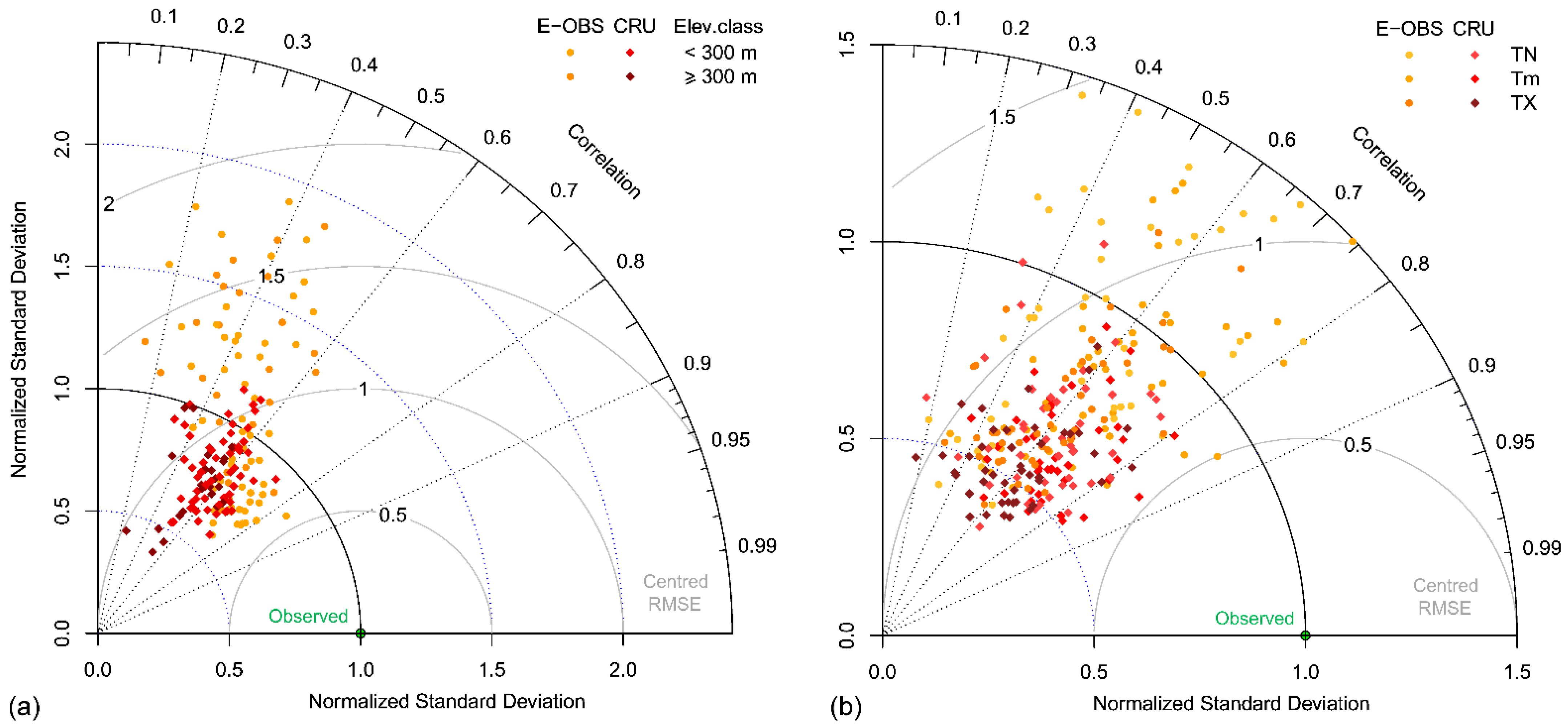
Taylor diagrams for total annual precipitation and annual mean, minimum and maximum temperature data extracted at station locations from the E-OBS (in orange) and CRU (in red) datasets are displayed in Figure 2. These graphs provide information on the datasets’ agreement with observations by simultaneously reporting three statistics, i.e., the normalized standard deviations of observed and extracted data as the radial distance from the graph origin, the centered root mean square difference (or error, RMSE), indicated by the distance from the point labeled as “observed”, located on the x-axis, and the Pearson correlation coefficient given by the azimuthal angle between the x-axis and the position vector [34].
Generally, both gridded datasets showed reasonable performances for most of the stations, with values of the correlation coefficient concentrated between 0.5 and 0.8. Regarding precipitation, CRU demonstrated to have a much closer resemblance with station data, while large deviations were observed for the E-OBS derived data in some sites, irrespective of their elevations (Figure 2a). A similar pattern, although with a more limited scatter, was also found for temperature data.
3.2. Trend Detection with the Use of the Different Datasets
After the preliminary investigation of the ability of gridded data products in replicating the climatic variables registered at the meteorological stations in the Apulia region, in this section we investigate to what extent the identified differences in the data sources affect the results of a trend analysis, in terms of sign, magnitude and significance of the detected change.
3.2.1. Precipitation Data
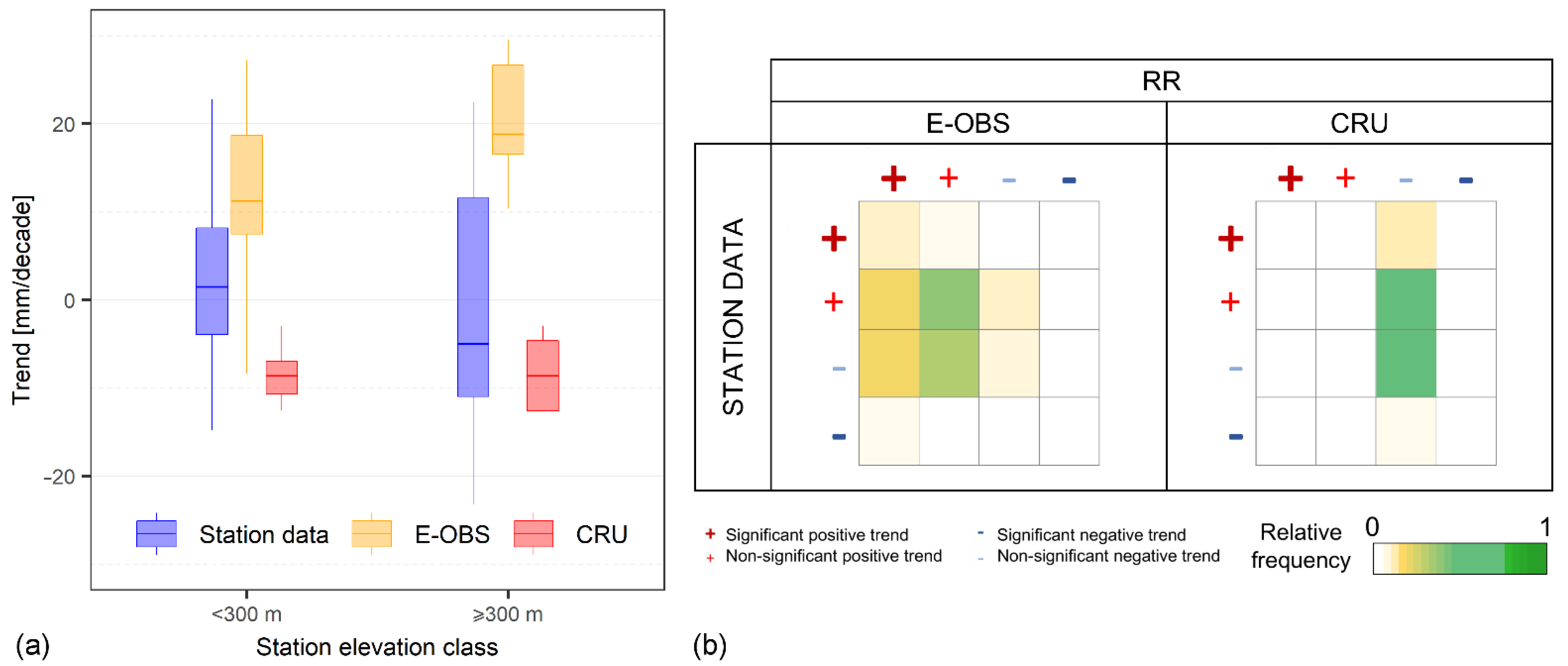
Results obtained for annual total precipitation for the period 1956–2019 are shown in Figure 3a, which summarizes, by means of boxplots, trend rates calculated at the individual stations for the different considered datasets. Along with trend magnitude, the normalized contingency matrices in Figure 3b give information on the possible mismatch of the trend sign and significance identified by using observational or extracted gridded data. The diagonal elements in the matrices represent the relative frequency of stations (i.e., number of stations over the total) for which the sign and significance of the trend assessed by using station data is equal to the one estimated with E-OBS or CRU data sources. Corresponding results at the seasonal scales are reported, for the sake of conciseness, in the Supplementary material (Figures S1 and S2).
On annual scale, about 95% of the gauging network exhibited a nonsignificant trend for total precipitation, almost equally distributed between positive and negative signs, with a larger variability in the results observed at the stations located above 300 m a.s.l. As for nonsignificant trends, E-OBS data correctly identified most of the few significant changes detected with station data, which were positive in four sites and negative in one. In particular, E-OBS data generally provided larger (positive) trend magnitudes, although with a variability similar to the one of station data, less evident at hilly locations. Differently, CRU data depicted a scenario of general nonsignificant reduction in total precipitation, with more spatially homogeneous rates of changes, as a consequence of the lower resolution of the dataset, which implies a smoothing of the local differences that are instead captured by the other two data sources. The seasonal analysis (Figures S1 and S2) indicated that the nonsignificant changes in rainfall amounts registered at annual scale are mainly the result of weak reductions in winter, counterbalanced by generally equal weak positive increases in autumn and spring.
The analysis with station data then confirmed the weak changes in precipitation observed in neighboring areas of central and southern Italy over the last years, with a more evident reduction during the winter season [41,42,43,44,45,46,47]. This tendency was not captured by E-OBS data, which described nonsignificant positive trends in all seasons, while CRU data showed a better agreement with the pattern depicted by observational data, although with a markedly reduced variability in the results.
3.2.2. Temperature Data
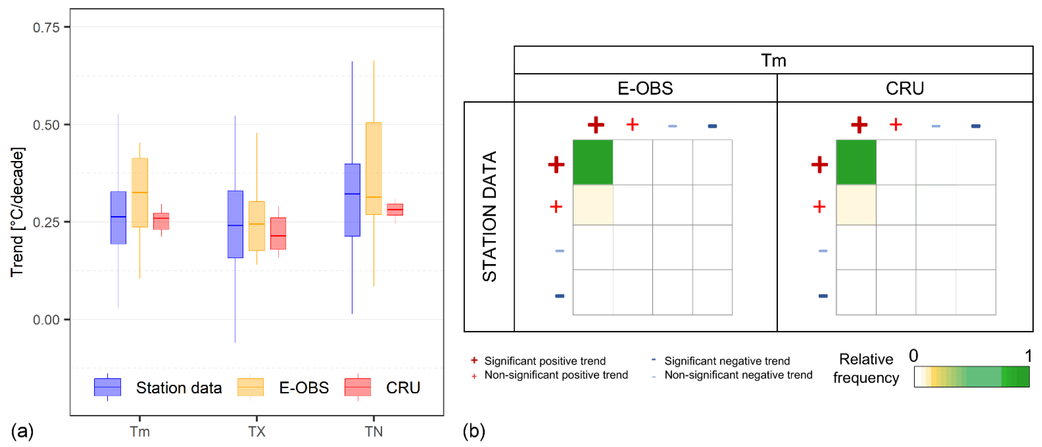
The results of trend analysis applied to annual mean, maximum and minimum temperatures, considering the different data sources, are summarized in Figure 4 and Figure S3, which clearly denote widespread warming tendencies in the Apulia region over the period 1956–2019. In particular, Tm showed a well-defined spatial pattern, with significant positive trends detected in almost 100% of the sites by the three selected databases (Figure 4b). However, some differences are evident in terms of trend magnitude, as visible in Figure 4a, which shows a larger rate of warming detected by E-OBS data (median trend magnitude for Tm: +0.33 °C/decade); the variability of trend rates identified by observational data was quite similar, although with a generally lower magnitude (median value of the trend for Tm: +0.27 °C/decade), comparable to the one identified by CRU data, which, as expected, was characterized by a less variable trend intensity. Figure 4 indicates that minimum temperature experienced a greater rate of warming than maximum temperature, confirmed by all the datasets, with observational and E-OBS data providing similar results, ranging from a median of about +0.24 °C/decade for TX to +0.32 °C/decade for TN, while CRU data reported slightly smaller rates of changes (+0.21 and +0.28 °C/decade for TX and TN, respectively).
Overall, trend magnitudes calculated in this study for Tm are consistent with previous findings on climate evolution observed during the last decades in Mediterranean countries [4,20,48,49] and in other Italian regions, as demonstrated, for instance, by Viola et al. [50] and Appiotti et al. [51], who described a +0.40 and +0.20 °C/decade increase for mean annual temperature in the Sicily and Marche regions, respectively.
Some of previous studies described for southern Europe a general more intense increase in the hot-tail (i.e., related to TX) of temperature distribution [45,52,53,54,55,56,57,58]. However, also depending on the different considered periods of analysis [16], this was confirmed not to be true in any region, as shown at larger spatial scales by Donat et al. [59], Fischer and Knutti [60] and Lorenz et al. [61], or by Bartolini et al. [62] and Caloiero et al. [63] for the Tuscany and Calabria regions of Italy, as well in the present study, which then confirmed spatially heterogenous patterns experienced by warming maximum and minimum temperatures over the globe.
Results of the seasonal analysis (Figures S4 and S5) revealed that the general increase in temperature detected at the annual scale is primarily due to a strong warming in summer and spring. Indeed, in these seasons, almost the whole set of stations exhibited significant positive signs for Tm, TX and TN. In particular, the maximum seasonal temperature trends were observed in summer, when the average temperature rise for Tm was estimated to be about +0.38 °C/decade, with similar values found between the different datasets, while spring reported an average change of about +0.27°/decade. Trend pattern in the cold half of the year was instead slightly more complex, but always characterized by prevailing positive signs, which were significant in less than 40% of the stations, considering observational data. For winter and autumn temperatures, CRU data tended to detect less significant positive trends, leading to generally lower trend magnitudes, as opposed to E-OBS data, which indicated the maximum rates of changes, particularly evident in the colder seasons. Similar considerations can be drawn for winter and autumn TX and TN, with the only exception for TNwin that showed the most noticeable differences in the results obtained with the selected data sources, as evident from Figure S4 and from the contingency matrix in Figure S5.
The described results are consistent with previous findings in the literature pointing out the summer nature of recent warming over southern Europe [45,52,53,54,56,58,62,64,65,66]. In addition, the more intense warming detected here by E-OBS data is in line with the results of Krauskopf and Huth [11], who described a similar pattern in Europe and explained these differences by inhomogeneities existing in the E-OBS gridded dataset, thus highlighting the need for a continuous validation of these large-scale data products versus point observations.
3.3. Aridity Classification and Trends
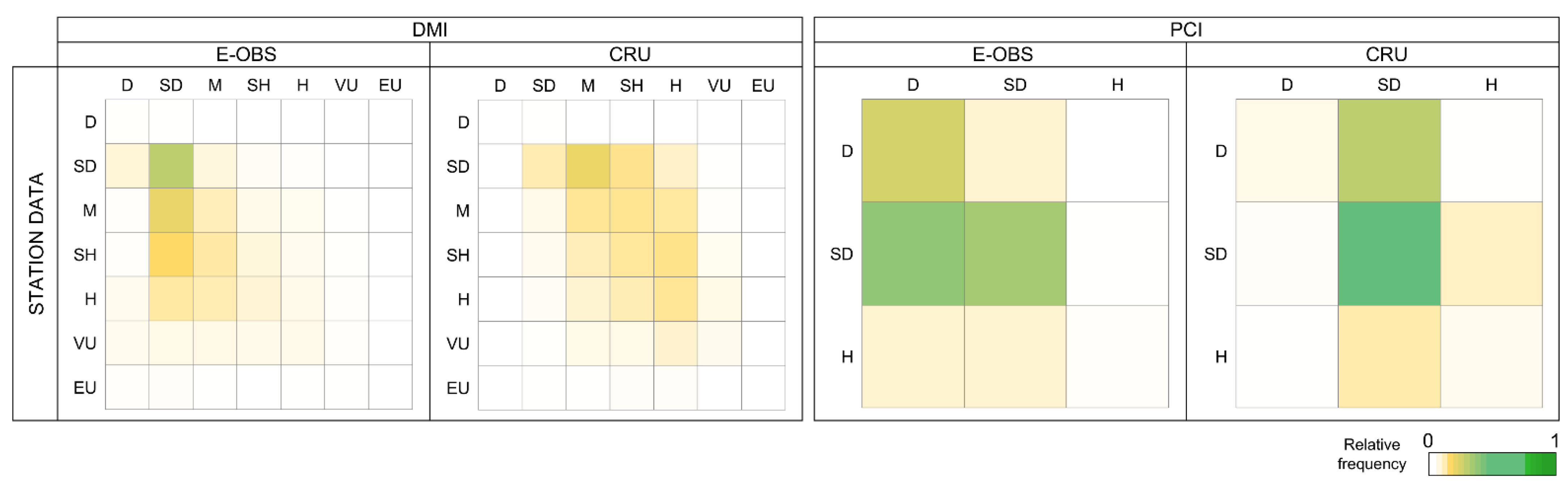
Figure 5 summarizes, by means of normalized contingency matrices, the results regarding the ability of the E-OBS and CRU datasets in identifying the aridity conditions experienced during the 1956–2019 period in the considered locations of the Apulia region, according to the De Martonne and Pinna combinative aridity classification (Table 1), thus providing information on their ability to represent the interannual and spatial variability of precipitation and temperature time series, combined into a single index. In detail, the colors in the cells of the matrices indicate the (relative) number of years, for the whole gauging network, which were labelled under a specific class considering station and gridded (E-OBS or CRU) data.
Considering the DMI, it can be noted that the E-OBS fairly captured the frequent semi-dry (SD) conditions experienced in the region, although some deviations toward Mediterranean (M) and semi-humid (SH) climates were not fully detected. A similar ability was observed also in terms of PCI, with the most frequent SD condition often correctly detected, with, however, some differences toward a drier climate indicated by E-OBS.
Larger dispersion is visible in the performance of the lower resolution CRU data for the DMI, with classification types provided by it that tended to be shifted toward more humid conditions. In terms of PCI, also in this case, the frequent SD years were instead mostly recognized, although with dry (D) conditions often misinterpreted as SD.
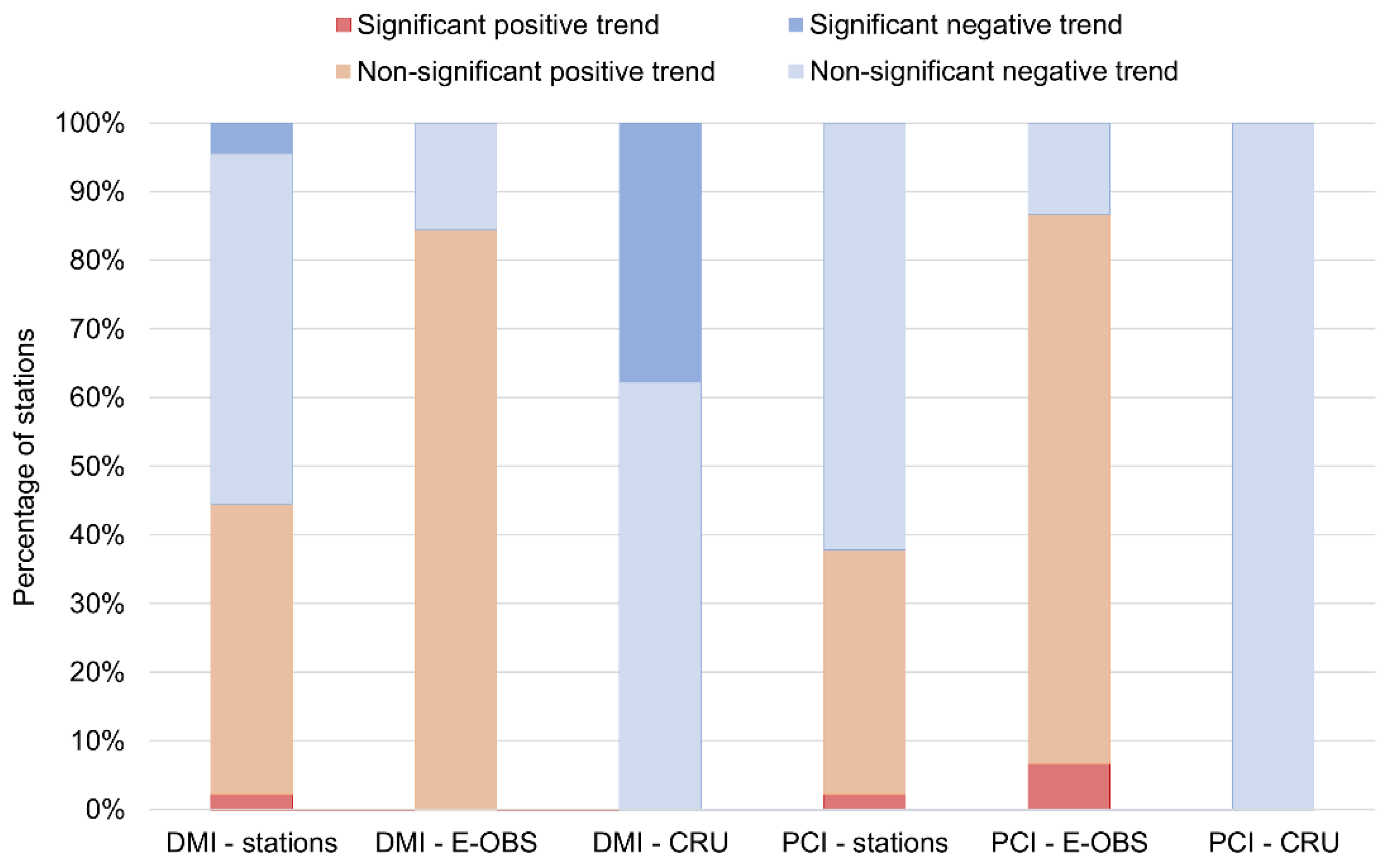
As regards the results for trends in the time series of the De Martonne and Pinna aridity indices, Figure 6 reveals no substantial changes in the Apulia region, where almost all considered locations experienced nonsignificant trends in the DMI and PCI over the 1956–2019 period.
This scenario seems to be confirmed by all the three datasets, although with some evident differences in the sign of detected changes, especially for the CRU data, which indicated only reductions in both DMI and PCI, differently from E-OBS and station data, for which a large number of positive signs are evident. By analyzing Figure 3, Figure 4 and Figure 6 it is apparent that the general stability in the aridity conditions is the combined effect of a significant, intense warming which is not, however, accompanied by a comparable change (i.e., reduction) in precipitation that could lead toward a more arid climate, as also described in other Mediterranean and central European regions [67,68,69,70,71].
4. Conclusions
The results of this study can contribute to improve knowledge of climate evolution over Italy and the wider Mediterranean basin in the past decades (1956–2019) and to provide important information on the accuracy of climatic gridded data products in resembling in situ observations in a climate-vulnerable region of southern Europe.
In detail, considering observational data, the following results were pointed out:
- Annual precipitation exhibited a widespread nonsignificant change in most of the gauging network, with a larger variability observed at hilly sites; this is the result of a weak precipitation reduction in winter, compensated for by similar weak positive increases in autumn and spring.
- Almost all the meteorological stations in the Apulia region experienced a significant warming over the considered period of analysis. The mean annual temperature registered a significant increase at a median rate of +0.27 °C/decade and the largest contribution to this increase was detected in the warm season, with a calculated median change of +0.38 °C/decade in summer. In particular, minimum temperatures registered a greater rate of warming than maximum temperatures.
- In terms of aridity classification, “dry” and “semi-dry” were the prevalent climate conditions experienced in the considered locations of the region, with no significant changes detected over the considered time period.
Regarding the ability of the considered gridded data products in resembling the above-mentioned results, this study revealed that they reasonably reproduced the observed trend patterns (i.e., sign), although with deviations evident in the estimation of trend magnitude and variability, thus allowing only general indications on the spatial–temporal evolution of temperature and precipitation parameters in the Apulia region. In particular, less accurate results were identified for precipitation data, in line with the expectations based on the larger spatial variability characterizing this parameter, if compared to temperature’s one.
Moreover, it was found that both E-OBS and, to a lesser extent, CRU data were mostly able to identify the climatic conditions experienced in the region, although with some evident deviations, which are the result of the combined effect of the inaccuracies present in both gridded precipitation and temperature data.
Therefore, the main conclusion of this study was that gridded datasets, especially for complex topographic and/or climatic regions, should be used with caution or only after a preliminary evaluation against observational data before any climatological application to ensure a proper reliability.
Supplementary Materials
The Supplement can be downloaded at: https://www.mdpi.com/article/10.3390/w14142203/s1. Table S1. Meteorological stations considered in the study. Figure S1. Calculated trend rates for seasonal precipitation using the three considered databases. Figure S2. Normalized contingency matrices for detected trend sign for seasonal precipitation using the three considered databases. Figure S3. Normalized contingency matrices for detected trend signs for annual maximum (TX) and minimum (TN) temperatures using the three considered databases. Figure S4. Calculated trend rates for seasonal mean (Tm), maximum (TX) and minimum (TN) temperatures using the three considered databases. Figure S5. Normalized contingency matrices for detected trend signs for seasonal mean (Tm), maximum (TX) and minimum (TN) temperatures using the three considered databases.
Author Contributions
Conceptualization, A.R.S.; methodology, A.R.S. and M.D.B.; formal analysis, A.R.S. and L.M.; investigation, A.R.S., L.M. and M.D.B.; data curation, A.R.S. and L.M.; writing—original draft preparation, A.R.S.; writing—review and editing, A.R.S. and M.D.B.; visualization, A.R.S. All authors have read and agreed to the published version of the manuscript.
Funding
This research received no external funding.
Institutional Review Board Statement
Not applicable.
Informed Consent Statement
Not applicable.
Data Availability Statement
The data used in this study are available at the following links: observational data: https://protezionecivile.puglia.it/centro-funzionale-decentrato/rete-di-monitoraggio/annali-e-dati-idrologici-elaborati/ (accessed on 18 May 2022); E-OBS data: https://surfobs.climate.copernicus.eu/dataaccess/access_eobs.php (accessed on 18 May 2022); CRU data: https://crudata.uea.ac.uk/cru/data/hrg/ (accessed on 18 May 2022).
Acknowledgments
The authors thank the “Centro Funzionale Decentrato della Protezione Civile della Regione Puglia” for providing the observational dataset of temperature and precipitation over the region. We also acknowledge the E-OBS dataset from the EU-FP6 project UERRA (https://www.uerra.eu, accessed on 18 May 2022) and the Copernicus Climate Change Service, and the data providers in the ECA&D project (https://www.ecad.eu, accessed on 18 May 2022), as well as the Climatic Research Unit (University of East Anglia) and NCAS for the CRU dataset.
Conflicts of Interest
The authors declare no conflict of interest.
References
- IPCC. Summary for Policymakers. In Climate Change 2021: The Physical Science Basis; Contribution of Working Group I to the Sixth Assessment Report of the Intergovernmental Panel on Climate Change; Masson-Delmotte, V., Zhai, P., Pirani, A., Connors, S.L., Péan, C., Berger, S., Caud, N., Chen, Y., Goldfarb, L., Gomis, M.I., et al., Eds.; Cambridge University Press: Cambridge, UK, 2021. [Google Scholar]
- Tapiador, F.J.; Turk, F.J.; Petersen, W.; Hou, A.Y.; García-Ortega, E.; Machado, L.A.; Angelis, C.F.; Salio, P.; Kidd, C.; Huffman, G.J.; et al. Global precipitation measurement: Methods, datasets and applications. Atmos. Res. 2012, 104, 70–97. [Google Scholar] [CrossRef]
- Brasseur, G.P.; Gallardo, L. Climate services: Lessons learned and future prospects. Rev. Geophys. 2018, 4, 79–89. [Google Scholar] [CrossRef] [Green Version]
- Klein Tank, A.M.G.; Wijngaard, J.B.; Können, G.P.; Böhm, R.; Demarée, G.; Gocheva, A.; Mileta, M.; Pashiardis, S.; Hejkrlik, L.; Kern-Hansen, C.; et al. Daily dataset of 20th-century surface air temperature and precipitation series for the European Climate Assessment. Int. J. Climatol. 2002, 22, 1441–1453. [Google Scholar] [CrossRef]
- Haylock, M.R.; Hofstra, N.; Klein Tank, A.M.G.; Klok, E.J.; Jones, P.D.; New, M. A European daily high-resolution gridded data set of surface temperature and precipitation for 1950–2006. J. Geophys. Res. 2008, 113, D20119. [Google Scholar] [CrossRef] [Green Version]
- Osborn, T.J.; Jones, P.D. The CRUTEM4 land surface air temperature data set: Construction, previous versions and dissemination via Google Earth. Earth Sci. Syst. Data 2014, 6, 61–68. [Google Scholar] [CrossRef] [Green Version]
- Hofstra, N.; Haylock, M.; New, M.; Jones, P.D. Testing E-OBS European high-resolution gridded data set of daily precipitation and surface temperature. J. Geophys. Res. Atmos. 2009, 114, D21101. [Google Scholar] [CrossRef]
- Kyselý, J.; Plavcová, E. A critical remark on the applicability of E-OBS European gridded temperature data set for validating control climate simulations. J. Geophys. Res. Atmos. 2010, 115, D23118. [Google Scholar] [CrossRef]
- Faiz, M.A.; Liu, D.; Fu, Q.; Sun, Q.; Li, M.; Baig, F.; Li, T.; Cui, S. How accurate are the performances of gridded precipitation data products over Northeast China? Atmos. Res. 2018, 211, 12–20. [Google Scholar] [CrossRef]
- Musie, M.; Sen, S.; Srivastava, P. Comparison and evaluation of gridded precipitation datasets for streamflow simulation in data scarce watersheds of Ethiopia. J. Hydrol. 2019, 579, 124168. [Google Scholar] [CrossRef]
- Krauskopf, T.; Huth, R. Temperature trends in Europe: Comparison of different data sources. Theor. Appl. Climatol. 2020, 139, 1305–1316. [Google Scholar] [CrossRef]
- Yao, J.; Chen, Y.; Yu, X.; Zhao, Y.; Guan, X.; Yang, L. Evaluation of multiple gridded precipitation datasets for the arid region of northwestern China. Atmos. Res. 2020, 236, 104818. [Google Scholar] [CrossRef]
- Tanarhte, M.; Hadjinicolaou, P.; Lelieveld, J. Intercomparison of temperature and precipitation data sets based on observations in the Mediterranean and the Middle East. J. Geophys. Res. Atmos. 2012, 117, D12102. [Google Scholar] [CrossRef]
- Newman, A.J.; Clark, M.P.; Craig, J.; Nijssen, B.; Wood, A.; Gutmann, E.; Mizukami, N.; Brekke, L.; Arnold, J.R. Gridded ensemble precipitation and temperature estimates for the contiguous United States. J. Hydrometeorol. 2015, 16, 2481–2500. [Google Scholar] [CrossRef]
- Walton, D.; Hall, A. An assessment of high-resolution gridded temperature datasets over California. J. Clim. 2018, 31, 3789–3810. [Google Scholar] [CrossRef]
- Curci, G.; Guijarro, J.A.; Di Antonio, L.; Di Bacco, M.; Di Lena, B.; Scorzini, A.R. Building a local climate reference dataset: Application to the Abruzzo region (Central Italy), 1930–2019. Int. J. Climatol. 2021, 41, 4414–4436. [Google Scholar] [CrossRef]
- Sidău, M.R.; Croitoru, A.E.; Alexandru, D.E. Comparative Analysis between Daily Extreme Temperature and Precipitation Values Derived from Observations and Gridded Datasets in North-Western Romania. Atmosphere 2021, 12, 361. [Google Scholar] [CrossRef]
- Giorgi, F.; Lionello, P. Climate change projections for the Mediterranean region. Global Planet. Change 2008, 63, 90–104. [Google Scholar] [CrossRef]
- Norrant, C.; Douguédroit, A. Monthly and daily precipitation trends in the Mediterranean (1950–2000). Theor. Appl. Climatol. 2006, 83, 89–106. [Google Scholar] [CrossRef]
- Trenberth, K.E.; Jones, P.D.; Ambenje, P.; Bojariu, R.; Easterling, D.; Klein Tank, A.; Parker, D.; Rahimzadeh, F.; Renwick, J.A.; Rusticucci, M.; et al. Observations: Surface and Atmospheric Climate Change. In Climate Change 2007: The Physical Science Basis; Contribution of Working Group I to the Fourth Assessment Report of the Intergovernmental Panel on Climate Change; Solomon, S., Qin, D., Manning, M., Chen, Z., Marquis, M., Averyt, K.B., Tignor, M., Miller, H.L., Eds.; Cambridge University Press: Cambridge, UK; New York, NY, USA, 2007. [Google Scholar]
- Alpert, P.; Krichak, S.O.; Shafir, H.; Haim, D.; Osetinsky, I. Climatic trends to extremes employing regional modeling and statistical interpretation over the E. Mediterranean. Global Planet. Change 2008, 63, 163–170. [Google Scholar] [CrossRef]
- Philandras, C.M.; Nastos, P.T.; Kapsomenakis, J.; Douvis, K.C.; Tselioudis, G.; Zerefos, C.S. Long term precipitation trends and variability within the Mediterranean region. Nat. Hazards Earth Syst. Sci. 2011, 11, 3235–3250. [Google Scholar] [CrossRef] [Green Version]
- Kostopoulou, E.; Giannakopoulos, C.; Hatzaki, M.; Tziotziou, K. Climate extremes in the NE Mediterranean: Assessing the E-OBS dataset and regional climate simulations. Clim. Res. 2012, 54, 249–270. [Google Scholar] [CrossRef]
- Turco, M.; Zollo, A.L.; Ronchi, C.; De Luigi, C.; Mercogliano, P. Assessing gridded observations for daily precipitation extremes in the Alps with a focus on northwest Italy. Nat. Hazards Earth Syst. Sci. 2013, 13, 1457–1468. [Google Scholar] [CrossRef] [Green Version]
- Dumitrescu, A.; Birsan, M.V. ROCADA: A gridded daily climatic dataset over Romania (1961–2013) for nine meteorological variables. Nat. Hazards 2015, 78, 1045–1063. [Google Scholar] [CrossRef]
- Marini, G.; Fontana, N.; Mishra, A.K. Investigating drought in Apulia region, Italy using SPI and RDI. Theor. Appl. Climatol. 2019, 137, 383–397. [Google Scholar] [CrossRef]
- Polemio, M.; Casarano, D. Climate change, drought and groundwater availability in southern Italy. Geol. Soc. Lond. Spec. Publ. 2008, 288, 39–51. [Google Scholar] [CrossRef] [Green Version]
- Ladisa, G.; Todorovic, M.; Liuzzi, G.T. A GIS-based approach for desertification risk assessment in Apulia region, SE Italy. Phys. Chem. Earth 2012, 49, 103–113. [Google Scholar] [CrossRef]
- Polemio, M.; Lonigro, T. Climate variability and landslide occurrence in Apulia (Southern Italy). In Landslide Science and Practice; Margottini, C., Canuti, P., Sassa, K., Eds.; Springer: Berlin/Heidelberg, Germany, 2013; pp. 37–41. [Google Scholar]
- Lionello, P.; Congedi, L.; Reale, M.; Scarascia, L.; Tanzarella, A. Sensitivity of typical Mediterranean crops to past and future evolution of seasonal temperature and precipitation in Apulia. Reg. Environ. Change 2014, 14, 2025–2038. [Google Scholar] [CrossRef]
- World Meteorological Organization. Guide to Meteorological Instruments and Methods of Observation; World Meteorological Organization: Geneva, Switzerland, 2008. [Google Scholar]
- Cornes, R.C.; van der Schrier, G.; van den Besselaar, E.J.M.; Jones, P.D. An Ensemble Version of the E-OBS Temperature and Precipitation Datasets. J. Geophys. Res. Atmos. 2018, 123, 9391–9409. [Google Scholar] [CrossRef] [Green Version]
- Harris, I.; Osborn, T.J.; Jones, P.; Lister, D. Version 4 of the CRU TS monthly high-resolution gridded multivariate climate dataset. Sci. Data 2020, 7, 109. [Google Scholar] [CrossRef] [Green Version]
- Taylor, K.E. Summarizing multiple aspects of model performance in a single diagram. J. Geophys. Res. Atmos. 2001, 106, 7183–7192. [Google Scholar] [CrossRef]
- Mann, H.B. Nonparametric tests against trend. Econometrica 1945, 13, 245–259. [Google Scholar] [CrossRef]
- Kendall, M.G. Rank Correlation Methods; Griffin: London, UK, 1975. [Google Scholar]
- Sen, P.K. Estimates of the regression coefficient based on Kendall’s tau. J. Am. Stat. Assoc. 1968, 63, 1379–1389. [Google Scholar] [CrossRef]
- De Martonne, E. Traité de Géographie Physique, Vol I: Notions generales, climat, hydrographie. Geogr. Rev. 1925, 15, 336–337. [Google Scholar] [CrossRef]
- Zambakas, J. General Climatology; Department of Geology, National & Kapodistrian University of Athens: Athens, Greece, 1992. [Google Scholar]
- Baltas, E. Spatial distribution of climatic indices in northern Greece. Meteorol. Appl. 2007, 14, 69–78. [Google Scholar] [CrossRef]
- Piccarreta, M.; Capolongo, D.; Boenzi, F. Trend analysis of precipitation and drought in Basilicata from 1923 to 2000 within a southern Italy context. Int. J. Climatol. 2004, 24, 907–922. [Google Scholar] [CrossRef]
- Caloiero, T.; Coscarelli, R.; Ferrari, E.; Mancini, M. Precipitation change in southern Italy linked to global scale oscillation indexes. Nat. Hazards Earth Syst. Sci. 2011, 11, 1683–1694. [Google Scholar] [CrossRef]
- Brunetti, M.; Caloiero, T.; Coscarelli, R.; Gullà, G.; Nanni, T.; Simolo, C. Precipitation variability and change in the Calabria region (Italy) from a high resolution daily dataset. Int. J. Climatol. 2012, 32, 57–73. [Google Scholar] [CrossRef]
- Romano, E.; Preziosi, E. Precipitation pattern analysis in the Tiber River basin (central Italy) using standardized indices. Int. J. Climatol. 2013, 33, 1781–1792. [Google Scholar] [CrossRef]
- Scorzini, A.R.; Leopardi, M. Precipitation and temperature trends over central Italy (Abruzzo Region): 1951–2012. Theor. Appl. Climatol. 2019, 135, 959–977. [Google Scholar] [CrossRef]
- Caporali, E.; Lompi, M.; Pacetti, T.; Chiarello, V.; Fatichi, S. A review of studies on observed precipitation trends in Italy. Int. J. Climatol. 2021, 41, E1–E25. [Google Scholar] [CrossRef]
- Chiaravalloti, F.; Caloiero, T.; Coscarelli, R. The Long-Term ERA5 Data Series for Trend Analysis of Rainfall in Italy. Hydrology 2022, 9, 18. [Google Scholar] [CrossRef]
- Brunet, M.; Jones, P.D.; Sigró, J.; Saladié, O.; Aguilar, E.; Moberg, A.; Della Marta, P.M.; Lister, D.; Walther, A.; López, D. Temporal and spatial temperature variability and change over Spain during 1850–2005. J. Geophys. Res. Atmos. 2007, 112, D12117. [Google Scholar] [CrossRef] [Green Version]
- Brunetti, M.; Maugeri, M.; Monti, F.; Nanni, T. Temperature and precipitation variability in Italy in the last two centuries from homogenised instrumental time series. Int. J. Climatol. 2006, 26, 345–381. [Google Scholar] [CrossRef]
- Viola, F.; Liuzzo, L.; Noto, L.V.; Lo Conti, F.; La Loggia, G. Spatial distribution of temperature trends in Sicily. Int. J. Climatol. 2014, 34, 1–17. [Google Scholar] [CrossRef]
- Appiotti, F.; Krželj, M.; Russo, A.; Ferretti, M.; Bastianini, M.; Marincioni, F. A multidisciplinary study on the effects of climate change in the northern Adriatic Sea and the Marche region (central Italy). Reg. Environ. Change 2014, 14, 2007–2024. [Google Scholar] [CrossRef]
- Kostopoulou, E.; Jones, P.D. Assessment of climate extremes in the Eastern Mediterranean. Meteorol. Atmos. Phys. 2005, 89, 69–85. [Google Scholar] [CrossRef]
- Tomozeiu, R.; Pavan, V.; Cacciamani, C.; Amici, M. Observed temperature changes in Emilia-Romagna: Mean values and extremes. Clim. Res. 2006, 31, 217–225. [Google Scholar] [CrossRef]
- Toreti, A.; Desiato, F. Temperature trend over Italy from 1961 to 2004. Theor. Appl. Climatol. 2008, 91, 51–58. [Google Scholar] [CrossRef]
- Simolo, C.; Brunetti, M.; Maugeri, M.; Nanni, T.; Speranza, A. Understanding climate change-induced variations in daily temperature distributions over Italy. J. Geophys. Res. Atmos. 2010, 115, D22110. [Google Scholar] [CrossRef]
- Fioravanti, G.; Piervitali, E.; Desiato, F. Recent changes of temperature extremes over Italy: An index-based analysis. Theor. Appl. Climatol. 2016, 123, 473–486. [Google Scholar] [CrossRef]
- Scorzini, A.R.; Di Bacco, M.; Leopardi, M. Recent trends in daily temperature extremes over the central Adriatic region of Italy in a Mediterranean climatic context. Int. J. Climatol. 2018, 38, e741–e757. [Google Scholar] [CrossRef]
- Di Bacco, M.; Scorzini, A.R. Recent changes in temperature extremes across the north-eastern region of Italy and their relationship with large-scale circulation. Clim. Res. 2020, 81, 167–185. [Google Scholar] [CrossRef]
- Donat, M.G.; Alexander, L.V.; Yang, H.; Durre, I.; Vose, R.; Dunn, R.J.H.; Willett, K.M.; Aguilar, E.; Brunet, M.; Caesar, J.; et al. Updated analyses of temperature and precipitation extreme indices since the beginning of the twentieth century: The HadEX2 dataset. J. Geophys. Res. Atmos. 2014, 118, 2098–2118. [Google Scholar] [CrossRef]
- Fischer, E.M.; Knutti, R. Detection of spatially aggregated changes in temperature and precipitation extremes. Geophys. Res. Lett. 2014, 41, 547–554. [Google Scholar] [CrossRef]
- Lorenz, R.; Stalhandske, Z.; Fischer, E.M. Detection of a climate change signal in extreme heat, heat stress, and cold in Europe from observations. Geophys. Res. Lett. 2019, 46, 8363–8374. [Google Scholar] [CrossRef] [Green Version]
- Bartolini, G.; Di Stefano, V.; Maracchi, G.; Orlandini, S. Mediterranean warming is especially due to summer season. Evidences from Tuscany (central Italy). Theor. Appl. Climatol. 2012, 107, 279–295. [Google Scholar] [CrossRef]
- Caloiero, T.; Coscarelli, R.; Ferrari, E.; Sirangelo, B. Trend analysis of monthly mean values and extreme indices of daily temperature in a region of southern Italy. Int. J. Climatol. 2017, 37, 284–297. [Google Scholar] [CrossRef]
- Efthymiadis, D.; Goodess, C.M.; Jones, P.D. Trends in Mediterranean gridded temperature extremes and large-scale circulation influences. Nat. Hazards Earth Syst. Sci. 2011, 11, 2199–2214. [Google Scholar] [CrossRef]
- Piccarreta, M.; Lazzari, M.; Pasini, A. Trends in daily temperature extremes over the Basilicata region (southern Italy) from 1951 to 2010 in a Mediterranean climatic context. Int. J. Climatol. 2015, 35, 1964–1975. [Google Scholar] [CrossRef]
- Dong, B.; Sutton, R.T.; Shaffrey, L. Understanding the rapid summer warming and changes in temperature extremes since the mid-1990s over Western Europe. Clim. Dyn. 2017, 48, 1537–1554. [Google Scholar] [CrossRef] [Green Version]
- Spinoni, J.; Vogt, J.; Naumann, G.; Carrao, H.; Barbosa, P. Towards identifying areas at climatological risk of desertification using the Köppen–Geiger classification and FAO aridity index. Int. J. Climatol. 2015, 35, 2210–2222. [Google Scholar] [CrossRef] [Green Version]
- El Kenawy, A.M.; McCabe, M.F.; Vicente-Serrano, S.M.; Robaa, S.M.; Lopez-Moreno, J.I. Recent changes in continentality and aridity conditions over the Middle East and North Africa region, and their association with circulation patterns. Clim. Res. 2016, 69, 25–43. [Google Scholar] [CrossRef] [Green Version]
- Cheval, S.; Dumitrescu, A.; Birsan, M.V. Variability of the aridity in the South-Eastern Europe over 1961–2050. Catena 2017, 151, 74–86. [Google Scholar] [CrossRef]
- Gavrilov, M.B.; An, W.; Xu, C.; Radaković, M.G.; Hao, Q.; Yang, F.; Guo, Z.; Perić, Z.; Gavrilov, G.; Marković, S.B. Independent aridity and drought pieces of evidence based on meteorological data and tree ring data in Southeast Banat, Vojvodina, Serbia. Atmosphere 2019, 10, 586. [Google Scholar] [CrossRef] [Green Version]
- Ullah, S.; You, Q.; Sachindra, D.A.; Nowosad, M.; Ullah, W.; Bhatti, A.S.; Jin, Z.; Ali, A. Spatiotemporal changes in global aridity in terms of multiple aridity indices: An assessment based on the CRU data. Atmos. Res. 2022, 268, 105998. [Google Scholar] [CrossRef]
Figure 1.
Overview of the study area, with indication of the considered meteorological stations (reported in Table S1) and spatial coverage of the two gridded datasets (E-OBS and CRU) selected for the analysis.
Figure 1.
Overview of the study area, with indication of the considered meteorological stations (reported in Table S1) and spatial coverage of the two gridded datasets (E-OBS and CRU) selected for the analysis.

Figure 2.
Taylor diagrams for assessing the performances of the E-OBS and CRU datasets in resembling the observations at the selected sites in the Apulia region: (a) precipitation data; (b) temperature data.
Figure 2.
Taylor diagrams for assessing the performances of the E-OBS and CRU datasets in resembling the observations at the selected sites in the Apulia region: (a) precipitation data; (b) temperature data.

Figure 3.
Results of trend analysis for total annual precipitation (RR) using the three considered databases: (a) calculated trend rates; and (b) normalized contingency matrices for detected trend signs.
Figure 3.
Results of trend analysis for total annual precipitation (RR) using the three considered databases: (a) calculated trend rates; and (b) normalized contingency matrices for detected trend signs.

Figure 4.
Results of trend analysis for annual mean, maximum and minimum temperatures (Tm, TX and TN) using the three considered databases: (a) calculated trend rates; and (b) normalized contingency matrices for detected trend signs.
Figure 4.
Results of trend analysis for annual mean, maximum and minimum temperatures (Tm, TX and TN) using the three considered databases: (a) calculated trend rates; and (b) normalized contingency matrices for detected trend signs.

Figure 5.
Normalized contingency matrices for aridity classification using the three considered databases: De Martonne (DMI, left) and Pinna combinative index (PCI, right).
Figure 5.
Normalized contingency matrices for aridity classification using the three considered databases: De Martonne (DMI, left) and Pinna combinative index (PCI, right).

Figure 6.
Results of trend analysis for the time series of the De Martonne (DMI) and Pinna combinative (PCI) aridity indices based on the different selected datasets.
Figure 6.
Results of trend analysis for the time series of the De Martonne (DMI) and Pinna combinative (PCI) aridity indices based on the different selected datasets.


Table 1.
Climatic classification for the De Martonne (DMI) and Pinna combinative index (PCI).
| Index | Climate Type | Acronym | Index Value |
|---|---|---|---|
| DMI | Dry | D | DMI < 10 |
| Semi-dry | SD | 10 ≤ DMI < 20 | |
| Mediterranean | M | 20 ≤ DMI < 24 | |
| Semi-humid | SH | 24 ≤ DMI < 28 | |
| Humid | H | 28 ≤ DMI < 35 | |
| Very humid | VH | 35 ≤ DMI ≤ 55 | |
| Excessively humid | EH | DMI > 55 | |
| PCI | Dry | D | PCI < 10 |
| Semi-dry | SD | 10 ≤ PCI ≤ 20 | |
| Humid | H | PCI > 20 |
Publisher’s Note: MDPI stays neutral with regard to jurisdictional claims in published maps and institutional affiliations. |
© 2022 by the authors. Licensee MDPI, Basel, Switzerland. This article is an open access article distributed under the terms and conditions of the Creative Commons Attribution (CC BY) license (https://creativecommons.org/licenses/by/4.0/).
Share and Cite
MDPI and ACS Style
My, L.; Di Bacco, M.; Scorzini, A.R. On the Use of Gridded Data Products for Trend Assessment and Aridity Classification in a Mediterranean Context: The Case of the Apulia Region. Water 2022, 14, 2203. https://doi.org/10.3390/w14142203
AMA Style
My L, Di Bacco M, Scorzini AR. On the Use of Gridded Data Products for Trend Assessment and Aridity Classification in a Mediterranean Context: The Case of the Apulia Region. Water. 2022; 14(14):2203. https://doi.org/10.3390/w14142203
Chicago/Turabian StyleMy, Lorenzo, Mario Di Bacco, and Anna Rita Scorzini. 2022. "On the Use of Gridded Data Products for Trend Assessment and Aridity Classification in a Mediterranean Context: The Case of the Apulia Region" Water 14, no. 14: 2203. https://doi.org/10.3390/w14142203
Note that from the first issue of 2016, this journal uses article numbers instead of page numbers. See further details here.