
Robust Multi-Objective Design Optimization of Water Distribution System under Uncertainty


Faculty of Civil and Environmental Engineering, Technion—Israel Institute of Technology, Haifa 3200003, Israel
*
Author to whom correspondence should be addressed.
Water 2022, 14(14), 2199; https://doi.org/10.3390/w14142199
Submission received: 8 June 2022
/
Revised: 1 July 2022
/
Accepted: 7 July 2022
/
Published: 12 July 2022
(This article belongs to the Section Urban Water Management)
Abstract
:The multi-objective design optimization of water distribution systems (WDS) is to find the Pareto front of optimal designs of WDS for two or more conflicting design objectives. The most popular conflicting objectives considered for the design of WDS are minimization of cost and maximization of resilience index which are considered for the current study. Robust multi-objective optimization is to find the optimal set of the Pareto front considering demand is uncertain. The robustness is controlled by a single parameter that defines the size of the uncertainty set it can vary. The study explores ellipsoidal uncertainty set with different sizes and co-variance matrices. A combined simulation–optimization framework with a combination of self-adaptive multi-objective cuckoo search (SAMOCSA) and the fmincon optimization algorithm is proposed to solve the robust multi-objective design problem. The proposed algorithm is applied to medium and large WDS. The main contribution of this paper is to study the effect of demand uncertainty and the correlation on the WDS designs in a multi-objective framework. The study shows that the inclusion of correlation into the multi-objective design framework can significantly affect the optimal designs.
1. Introduction
A water distribution system (WDS) is a combination of multiple physical infrastructures that work in unison to provide high-quality water to the downstream customers at required pressures. This WDS is essential for every developed city, making it a critical infrastructure that must be accurately designed and well managed and maintained. The optimal design of these WDSs is a highly complex problem involving nonlinearity. This problem becomes even more complex when the system needs to be designed under uncertainty.
Water distribution system (WDS) design optimization is one of the most heavily researched areas in the water resources and hydraulics domain. The design of new water distribution networks was initially viewed as a least-cost optimization problem, with pipe diameters, tank characteristics and pump characteristics being the most commonly considered decision variables. This classical problem is often aimed at meeting the consumer nodes’ pressure requirements while minimizing the building’s cost or rehabilitating the system. While maintaining the minimum pressures at the nodes is a necessary design requirement, maintaining customer satisfaction throughout its design life is also essential. The measure of customer satisfaction under unfavorable conditions is termed system reliability. Even though there is no definite mathematical way to measure the system reliability, multiple researchers accepted and used the resilience index to measure WDS reliability. When we try to increase the network’s resilience, the networks become more complex, and construction costs also increase. To overcome this problem of optimizing multiple conflicting objectives simultaneously, multi-objective optimization has been introduced.
Multi-objective optimization has also been extensively explored in the WDS sector. The studies ranged from two objectives, three objectives and even six objectives. Prasad and Park [1] proposed designs that minimize cost and maximize resilience. Farmani et al. [2] proposed multiple designs for the Anytown WDS benchmark, considering cost and reliability as conflicting objectives. Kapelan et al. [3] considered minimization of design cost and maximization of the robustness of WDS [4,5,6,7,8] and have tried to improve the design Pareto fronts of cost and resiliency using different multi-objective metaheuristics. Wang et al. [9] used five different multi-objective algorithms and combined the results to propose the true Pareto fronts for many WDS benchmark networks considering cost and resilience index as conflicting objectives. All these studies have formulated their design problem assuming the parameters are deterministic. When applied to real-life networks, these designs often do not meet their design performance. Not accounting for the uncertainty involved in the design parameters is one of the reasons for their poor performance than expectations.
1.1. Optimization under Uncertainty
The most popular optimization under uncertainty approach is the probabilistic approach. In the probabilistic approach, an uncertain parameter is assumed as a random number associated with the assumed probability density function (PDF). The PDF is assumed to be based on an expert’s opinion or previous statistical data. The probabilistic analysis aims at obtaining the PDF of the output dependent variable based on the variations of the input uncertain independent variable. There are multiple techniques to approximate the output dependent variable’s PDF. The most common method used is sampling methods like Monte Carlo simulations (MCS) or Latin hypercube sampling (LHS). The major difference between these two sampling methods is that the sampling is completely random in MCS. The method requires a huge number of samples. In the LHS method, the sampling is performed in a more stratified manner, reducing the number of samples required. The other methods are analytical methods, where the variance of the output parameter is estimated around its mean value. The most common analytical-based methods are the first-order reliability method (FORM) and first-order second moment (FOSM).
Bargiela and Hainsworth [10] increased the accuracy of the nodal pressure head estimates and quantified the uncertainty by confidence bound analysis, and compared them with Monte Carlo simulations. Kretzmann and van Zyl [11] developed a software package named MoCaSim-II that uses MCS and WDS analysis software to estimate the relationship between system reliability and tank capacity. Pasha and Lansey [12,13] analyzed the impact of uncertainty in bulk and wall reaction coefficient, pipe diameters, pipe roughness and demands in the water quality estimates of the system using EPANET. They used Monte Carlo simulations to obtain the estimates. Sumer and Lansey [14] worked on estimating the effect of pipe roughness uncertainty on rehabilitation and expansion design decisions. They worked with a steady-state hydraulic simulation model. The parameter uncertainty was quantified through FOSM, and then the propagation of this input uncertainty on output uncertainty was also evaluated through a second FOSM. Stochastic formulation of the WDS design problem is first studied by Lansey et al. [15]. They assumed PDFs for the uncertain parameters and developed chance constraint formulations to handle the uncertainty. Xu and Goulter [16] formulated a single objective optimization problem considering the minimization of the design cost as the main objective. They added an additional constraint of system reliability, which is formulated as a chance constraint considering the demand as uncertainty. Kapelan et al. [3] proposed a stochastic least-cost design problem under uncertainty. They assumed a known PDF for the uncertain input parameter and the output uncertainty is analyzed using LHS technique, the proposed design model is then solved using a genetic algorithm (GA) and robust genetic algorithm and the results are then compared. Babayan et al. [17] replaced the Monte Carlo simulation (MCS) or any other sampling techniques by adding a margin of safety factor for pressure at nodes and assuming the fluctuations of heads at nodes are caused by uncertainty in demand. They then reformulated the stochastic formulation into a deterministic case and solved the design problem using GA. Babayan et al. [18] further extended this work by proposing two stochastic modeling approaches for least-cost design problems, the first approach was an integrated approach where the stochastic formulation is converted to the deterministic formulation and then the problem is solved using standard GA. The second modeling approach was the sampling approach, where the stochastic formulation was directly tackled using standard GA and LHS sampling techniques for uncertainty analysis. Perelman et al. [19,20] proposed two non-probabilistic approaches to solve the least-cost design problem. Both approaches used robust counterpart (RC) techniques combined with a cross-entropy optimization algorithm for solving the problem. The first approach was to consider that the demand uncertainty only affects the mass balance constraint and formulate the RC whereas the second approach considered the explicit formulation by carrying the uncertainty to the energy constraint as well. To apply the RC technique, the authors suggested a linear approximation for the head loss function and then used this linear surrogate to simplify the least-cost design problem formulation and then use robust optimization techniques to convert the uncertain formulation to tractable formulation and solve the problem using the single objective cross-entropy optimization algorithm.
1.2. Multi-Objective Optimization of WDS Design under Uncertainty
Kapelan et al. [21] proposed a multi-objective optimization problem with design cost minimization and system robustness as objectives. They considered nodal demands and pipe roughness as uncertain with a known PDF. They used Latin hypercube sampling to overcome the additional computational complexity that arises due to stochastic formulation. A modified NSGA-II algorithm is used for obtaining Pareto fronts. A two stage multi-objective optimization model was proposed by Giustolisi et al. [22]. The first stage was to obtain the solutions based on deterministic least cost design formulation using GA and then use the solutions obtained as the initial population set for solving the stochastic least-cost design formulation with two objectives one being the least cost and other being maximizing robustness using OPTIMOGA algorithm. LHS was used as the uncertainty analysis technique. They considered both demand and pipe roughness as uncertain in their formulation. Jung et al. [23] proposed a MOGA based stochastic problem formulation. The reliability is measured using two different approaches, the first being the variability of only the critical node and the second is to consider all the nodes variability. The results are compared using a disturbance index. They stated that the robustness is not achieved when only critical nodes are considered. A brief description of uncertainty-based studies in WDS design area are shown in Table 1.
Stochastic optimization methods have been extensively explored in the past to solve the least-cost design problem; later, it has also been explored to solve multi-objective design problem with the second objective being robustness or reliability of the design. Even though these design methodologies are reliable in terms of handling uncertainty, the heavy computational time and the uncertainty in the PDF assumptions reduced the practical application of these methodologies. Non-probabilistic optimization techniques proved to be much more reliable and faster in computation than stochastic formulations. Many non-probabilistic based optimization techniques were explored in the recent past in the water resource management sector [19,20,27,28,29,30,31,32]. Robust optimization techniques are one of the promising non-probabilistic techniques to handle uncertainty. These techniques are used to solve least cost design problem under uncertainty with single [20] and multiple loading conditions [32]. There are no reported studies that used non-probabilistic techniques to solve a multi-objective problem formulation of WDS design. The current study aims to fill this research gap. Minimization of design cost and maximization of resilience are considered as design objectives. A combination of robust optimization techniques and a self-adaptive multi-objective algorithm is proposed to solve this multi-objective WDS design under demand uncertainty. The proposed methodology is applied to a medium and large WDNs, and the results obtained are discussed.
2. Methodology
2.1. Robust Optimization
Robust optimization concepts can be easily explained through linear optimization problems, the uncertain linear optimization problem can be written as,
where x = is a vector of decision variables, a is a vector of coefficeints associated with objective fubnction, is a vector of uncertain coefficients associated with the ith constraint which can vary within the uncertainty set and is the right hand side parmeter of the constraint. where is the projection of uncertainty set U in the direction of ith dimension.
Based on the type of uncertainty set, the robust optimization formulations vary. For the current study, we look into ellipsoidal uncertainty sets. These ellipsoidal uncertainty sets have many advantages such as (a) they can be used to incorporate correlations between the uncertain variables, (b) it provides less conservative solutions than box uncertainty set (where the uncertain parameters can take worst values at the same time).
2.2. Ellipsoidal Uncertainty Set
Let us assume that for every ith constraint, can vary within the interval , where is the nominal value and is the maximum deviation from the nominal value.
For any uncertain coefficient with nominal value and covariance matrix , the ellipsoidal uncertainty can be defined using Mahalanobis distance in the form:
Here, correlation matrix, “u” is the perturbation vector, is the Euclidean norm, and “” is a value controlling the size of the ellipsoidal uncertainty set which is also referred to as the protection level Ben-Tal and Nemirovski [33].
So, for the problem defined in Equations (1) and (2), the robust equality formulation for the constraint in Equation (2) is as follows:
The solution for Equation (4) can be easily attained using Karush–Kuhn–Tucker (KKT) conditions to find that
By substituting the value of in the constraint we obtain,
As is a covariance matrix, we can use Cholesky decomposion to simply the LHS term in Equation (5). Assume , then the Equation (5) can be written as
In summary, we restrict all of the parameters from obtaining their worst-case values simultaneously by using an ellipsoid set.
2.3. Two-Objective Cost vs. Resilience Design of Water Distribution System
The optimal design of water distribution systems is an np-hard problem due to its large search space, discrete combinatorial nature and nonlinear and complex constraints. In the past, the optimal design of WDS was treated as a single objective optimization problem, where the optimal pipe diameters were obtained that minimize the overall construction cost of the WDS. Multiple scholars criticized this design method as a few of the designs obtained through this method lacked reliability [34,35,36]. The reliability of water distribution system can be estimated by surrogate measures. There have been many surrogate measures proposed and utilized in the past to estimate the reliability of WDS and also obtain reliable designs using multi-objective optimization algorithms. The surrogate measures can be categorized into entropy-based, power/energy-based and also the hybrid surrogate.
Entropy-based surrogate measures for reliability are initially proposed by Shannon et al. [37]. Redundancy or increase in multiple flow paths and flow uniformity can increase the entropy in WDS.
Power or energy-based surrogate measures are the most explored surrogate reliability measures in WDS. They use the total energy supplied to the systems by sources and pumps to determine the WDS’s resistance to pipe failures. Todini [38] proposed a resilience index indicator based on excess energy quantification in the system. Maximization of this resilience index ensures less energy is dissipated in the system flow due to friction enabling higher energy available at demand nodes that can be used to overcome abnormal network conditions.
“Optimizations based on resilience index and flow entropy revealed that the system optimized with resilience index was more reliable and cheaper in hydraulic failure conditions rather than mechanical” stated Gheisi et al. [39].
The energy efficiency index was proposed by Dziedzic and Karney [40]. Energy efficiency was defined as the ratio of the energy of water supplied to consumers to the total energy of water entering the WDS from sources, tanks and pumps. The performance index comprises four different indices (reliability, vulnerability, resilience, and connectivity), making it more comprehensive. Reliability was defined as the average of computed energy efficiencies over different scenarios of failure. Vulnerability was defined as the minimum energy efficiency that occurred in various failures. Resilience was defined as the average energy efficiency during the recovery period after failure. Connectivity was defined as the minimum percentage of delivered water to consumers during different failure scenarios, according to Gheisi et al. [39].
In addition to these surrogate measures, researchers have also used additional constraints like maintaining the system pressure and flow velocities [41] within specific limits to increase the reliability of the obtained system design
As most of the studies in the past used the resilience index as the reliability measure, we also used this resilience index metric as our second objective function for the current study. The final multi-objective problem formulation can be written as follows Equations (7)–(12):
Here —unit cost per length of pipe corresponding to the diameter, —set of design diameters, —length of pipe, np—number of pipes, —demand of node “I”, h—pressure head at node, —minimum pressure required, nr—number of reservoirs, —flow from reservoir “s”, —pressure head of reservoir “s”, npu—number of pumping units, —energy of pump “b”, —efficiency of the pump, nn—number of nodes in the network, = is the connectivity matrix of the network based on topology, —nonlinear elements representing the frictional resistance of the pipe, Q—Flow values in each pipe.
The Equation (10) represents the energy conservation constraint where is the head loss term which can be expanded as:
where , —pipe friction coefficient, = 1.852, a = 4.87 and is the Hazen–Willams coefficient.
2.4. Robust Optimization Formulation Considering Demand(q) as an Uncertain Variable
In this work, we assumed that consumer demands are uncertain, and we employ robust optimization formulations to obtain optimal designs under uncertainty. The proposed model is based on the correlated uncertainty model proposed by Perelman et al. [19].
For the explicit formulation of the constraints under demand uncertainty, a linear surrogate model is used to replace the head loss function Equation (12). This linear formulation of head loss within a domain underestimates the nodal heads within the range and overestimates outside the range (Perelman et al., 2013a)
This Equation (13) along with Equation (9) can be combinedly written as follows (Equation (15))
where is the inverse of the matrix , is of the size , is of size and , where is a given vector of fixed known heads.
From the Equation (15), the nodal heads ”h” can be computed as
Using this formulation, we can rewrite the optimization problem as
Now consider the Equations (18) and (19), the equation contains demand (q) as an uncertain parameter, the robust optimization formulation for this is assuming the demand varies in the uncertainty set and Then, as explained in the ellipsoidal robust optimization formulation (Equations (3)–(6)), we can write the formulation as follows.
Robust optimization formulation for resilience index, for simplifying the problem, let us assume that the network consists of only one source and no pumps. Then, the simplified resilience index equation can be written as:
The robust optimization formulation for the problem in Equation (21) is,
The resilience index formulation is still nonlinear with a form similar to quadratic over linear, but all the elements in the matrix are according to negative Perelman et al. [19]. The denominator is always positive as energy at the source is always greater than energy reached at the nodes , this problem will never be of the form quadratic over linear with the positive definite quadratic matrix.
In order to solve the optimization problem in Equation (22), an inbuilt nonlinear optimization algorithm in MATLAB named “fmincon” is used.
The overall robust multi-objective formulation used in this study is as follows:
3. Case Study
The proposed method is applied to the two standard benchmark problems (medium-sized network and large network). (1) Hanoi WDS proposed by Fujiwara and Khang [42], (2) large network extracted from Alperovits and Shamir [43].
3.1. Multi-Objective Optimization Method
Self-adaptive multi-objective cuckoo search algorithm (SAMOCSA) combined with the fmincon nonlinear optimization model is used to solve the robust multi-objective WDS design optimization problem. SAMOCSA is an improved version of the multi-objective cuckoo search that adapts the algorithm’s exploration and exploitation governing parameters at every iteration. This algorithm has been tested on the two-loop network, Hanoi network and Pamapur network (Indian network) for the deterministic multi-objective design problems of WDS. The complete details of the algorithm and its efficiency can be obtained from Pankaj et al. [7].
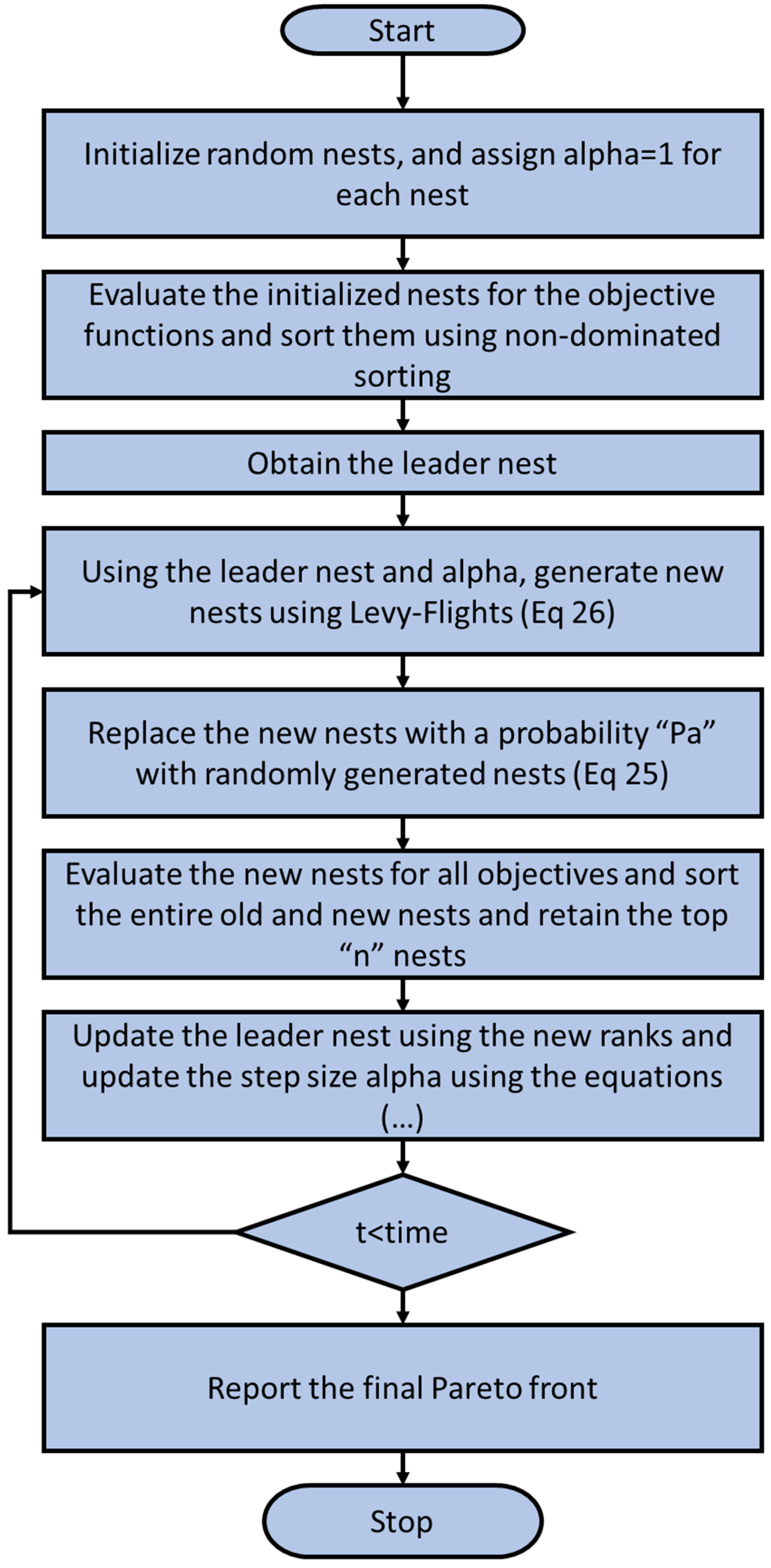
The flowchart of the working mechanism of SAMOCSA is shown in Figure 1. The first step is to initialize algorithm parameters, which generates the initial nests (population) using uniform random distribution within the search space, and also evaluates the generated random nests and store the corresponding objective function values. The next step is to obtain the leader nest, which belongs to the first Pareto front and has highest crowding distance after non-domination sorting of the initial nests. The non-domination sorting is inspired from the NSGA-II algorithm. The next step is to generate the new nests using Levy flight random walk and update the nests. Then, the new nests are replaced with generated nests with a discovering probability “Pa”. After updating the population, these steps are repeated until maximum number of iterations initialized at the start. The “Pa” value is dynamically adapted using the Equation (27). The step-length “alpha(α)” is updated using the current rank (Pareto front number) and crowding distance and also the nests in the first Pareto front. The step-length changes are based on the conditions shown below (Equation (28)).
Here belongs to set of nests, , rand—random number generated using uniform random distribution, is a function of leader nest and the Levy-flight parameter , —maximum value of the discovering probability (0.9), t—Iteration number, time—maximum number of iterations.
3.2. Case Study 1-Hanoi WDS
Hanoi WDS is a medium gravity-based WDS proposed by Fujiwara and Khang [42]. The network consists of 32 demand nodes and 34 pipes connected to a single source with a head of 100 m. The minimum pressure head required at every node is 30 m. The network needs to be designed with six different sized pipes. The unit cost corresponding to the available diameter are shown in Table 2. The full data for this example can be found in University of Exerter data files [44]
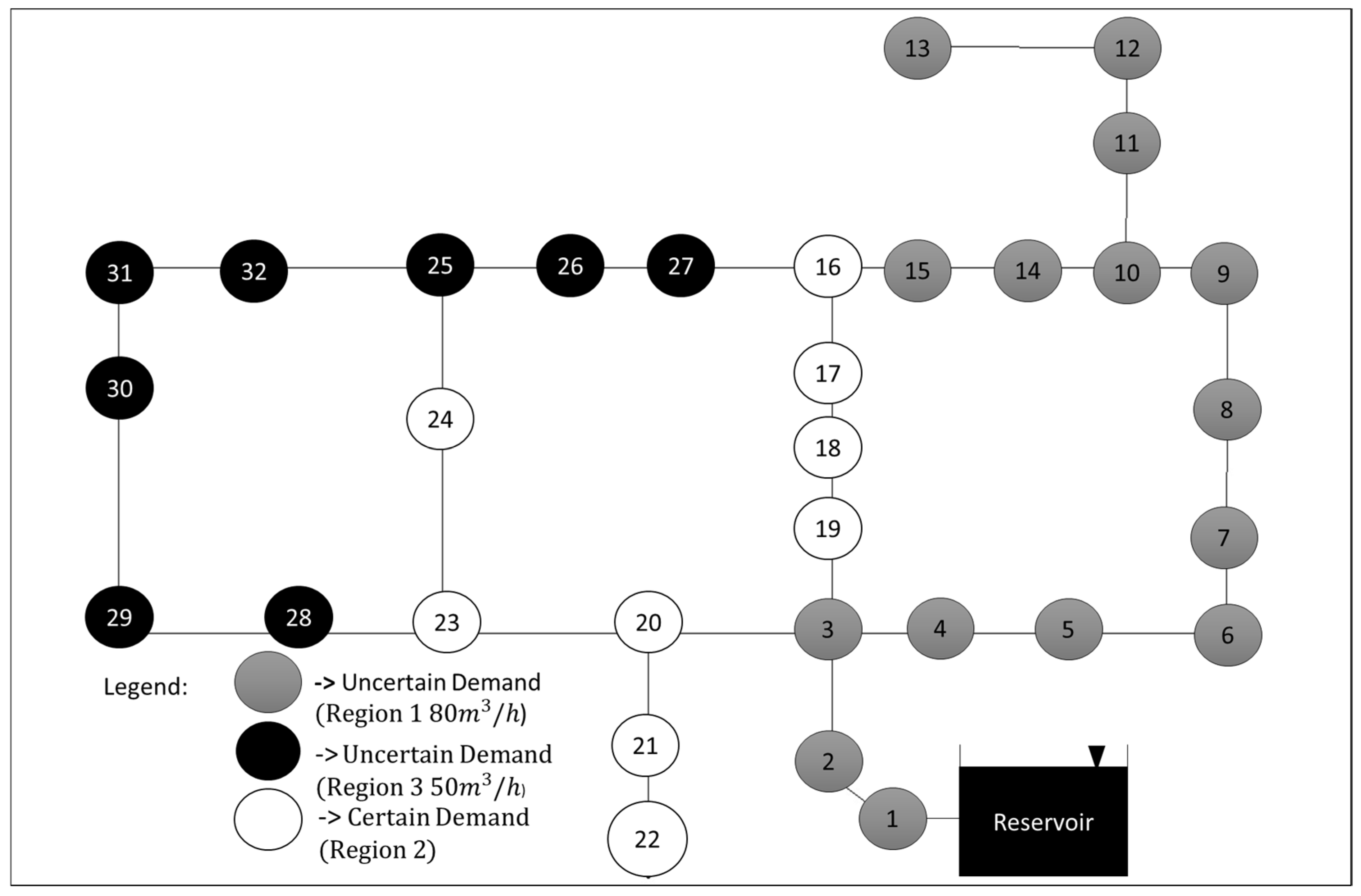
To model uncertainty in demands, the WDS nodes were partitioned into three demand regions: region 1—nodes 1:15, region 2—16:24, and region 3—25:32 (Figure 2). Demands in region 2 were assumed to be certain and in regions 1 and 3 as uncertain with a standard deviation of 12% from the mean demand of each region, (i.e., 80 and 50 (m3/h), respectively. Four different protection levels are studied . Furthermore, the correlation between the nodes within the region and the correlation between the regions are also altered. The intraregional correlation values are set to be and the interregional correlation varies between positive, no correlation and negative correlation . SAMOCSA algorithm is used to solve the outer design problem, and the fmincon algorithm is used to solve the nonlinear inner optimization problem for minimization of the resilience index within the demand search space.
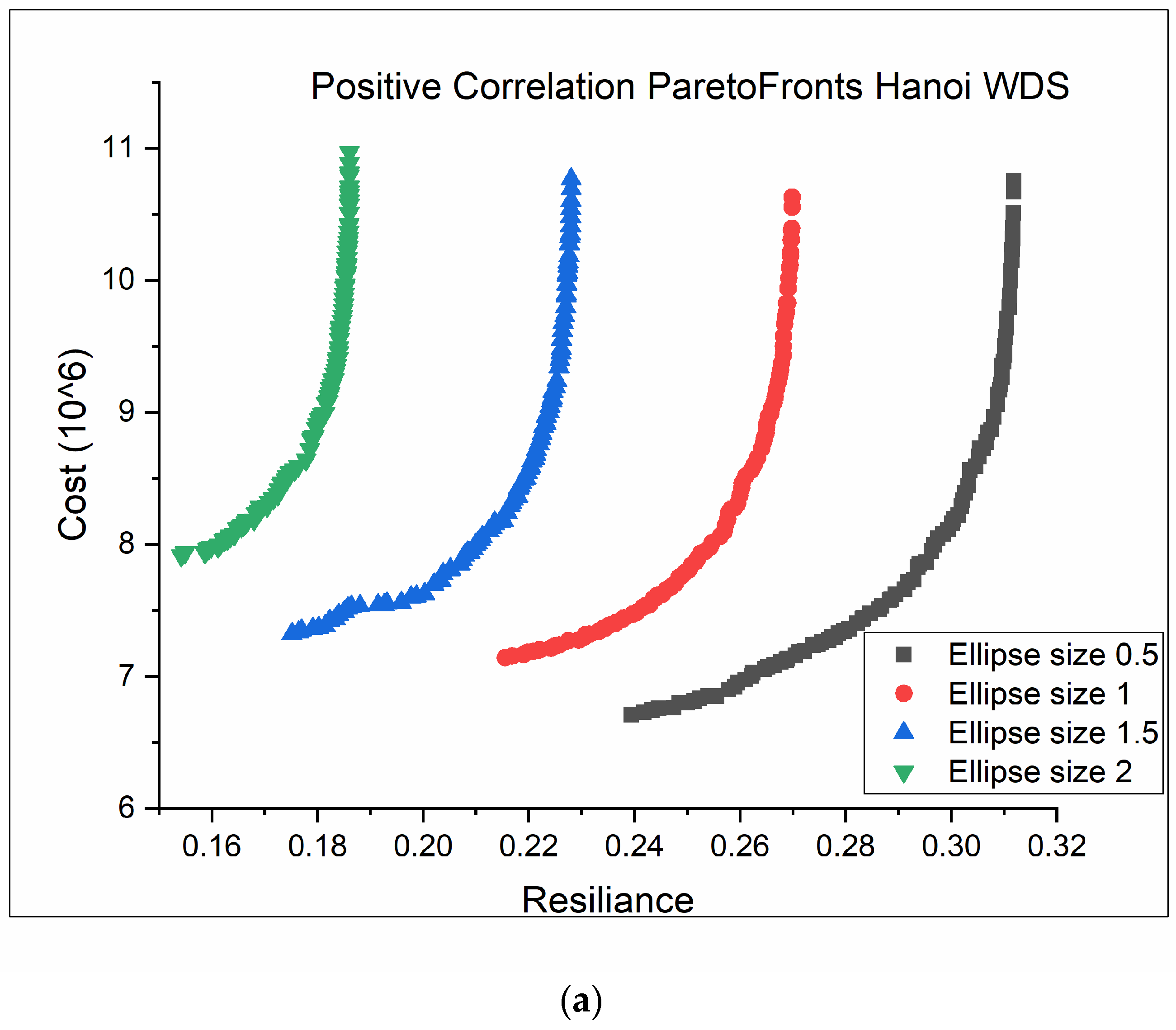
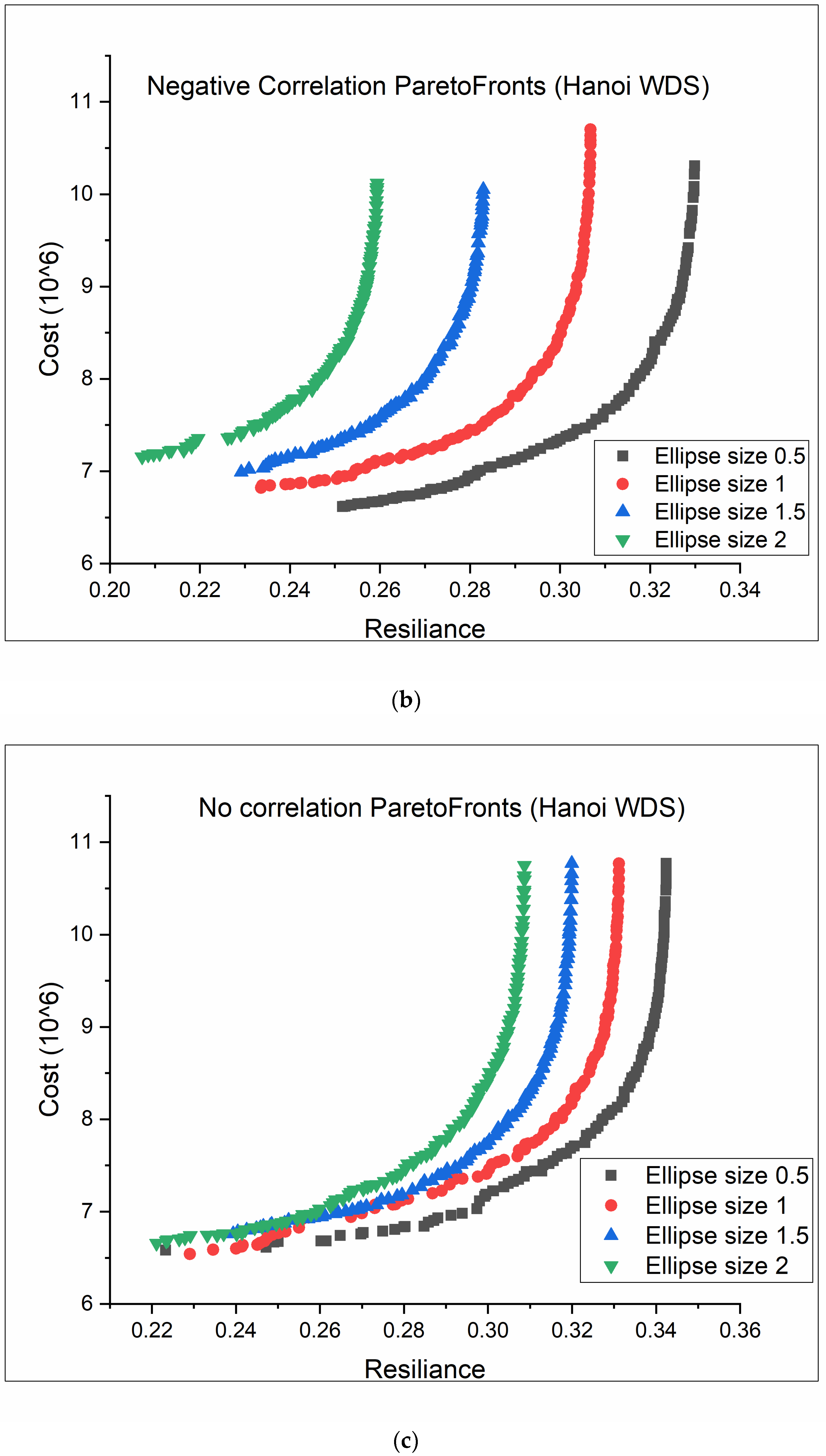
Figure 3a–c and Table 3 show the variation in the design Pareto fronts with changes in the uncertainty sets and correlation between the demands of consumer nodes. The Hanoi network is a low resilient network; the variation in protection levels significantly affects the design Pareto fronts can be inferred from the graphs. With the increase in the protection levels, higher design costs are required to satisfy even minimum resilience levels. Among the three cases, a positive correlation between the demands shows the highest effect on the designs, followed by negative and no correlation, respectively. For the no correlation case, the effect of an increase in the protection levels seems to have little variation in the cost for low resilient designs compared to high resilient designs.
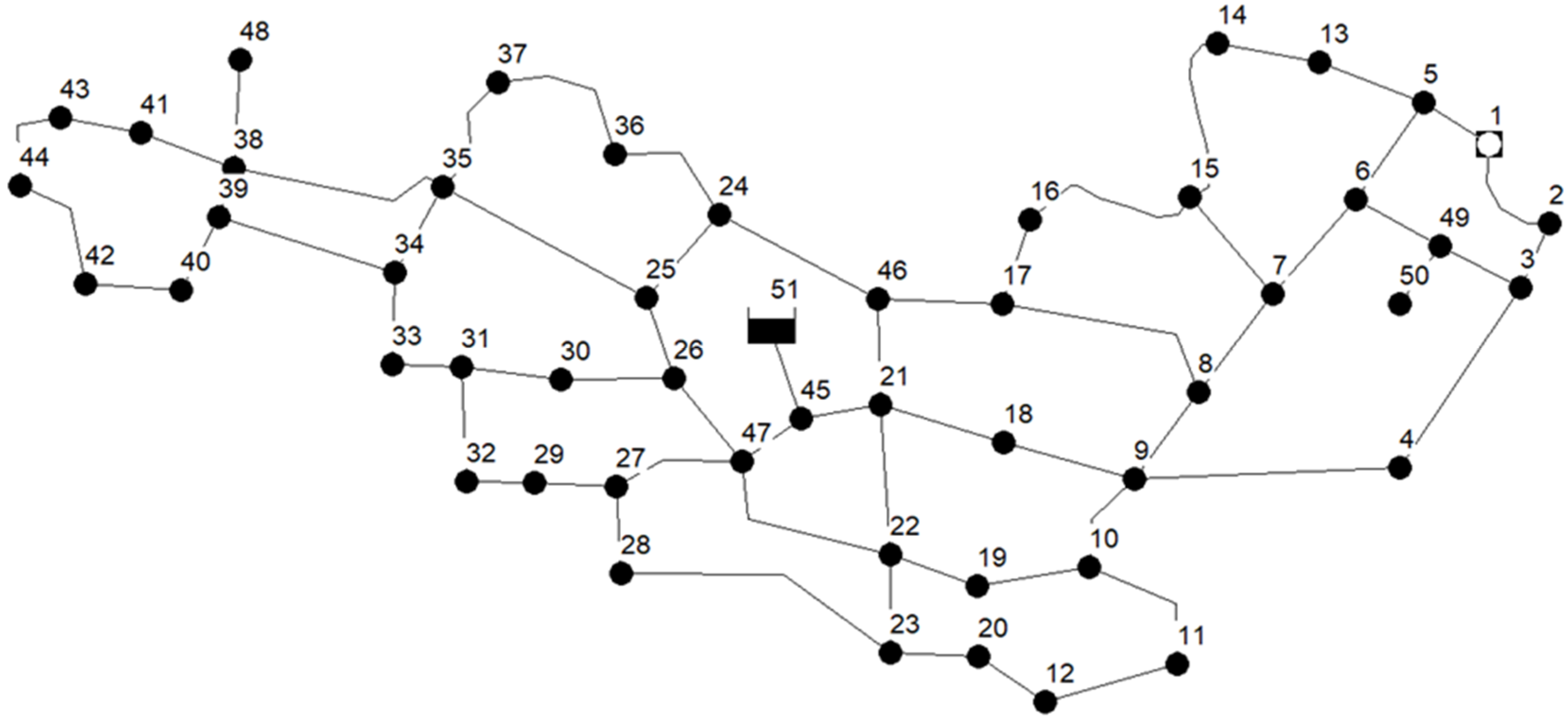
3.3. Case Study 2-Large Network
This network is a much larger network based on a real-life WDS (Figure 4) introduced by Alperovits and Shamir [43]. All the demand nodes are assumed to be uncertain with a specified covariance matrix. The network system is shown in Figure 3. The network consists of 52 nodes and 65 pipe segments. The two pumping stations in the original network are removed, and the reservoir head is increased to 410 m to balance the energy supplied by the pumps. The minimum pressure head required at every node is 30 m in addition to the elevation of the nodes. The design search space consists of 11 different pipe sizes (Table 4) for each pipe segment. The Hazen–Williams coefficient is fixed at 130.
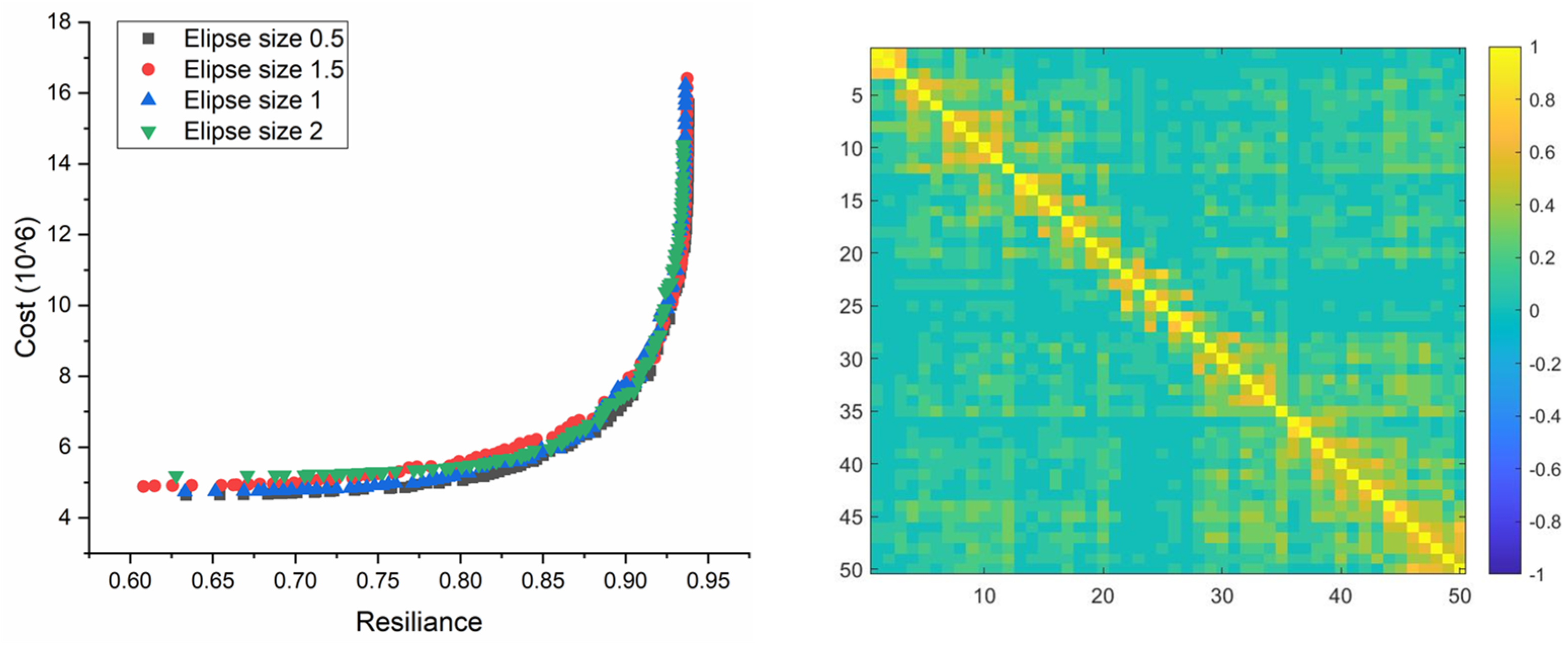
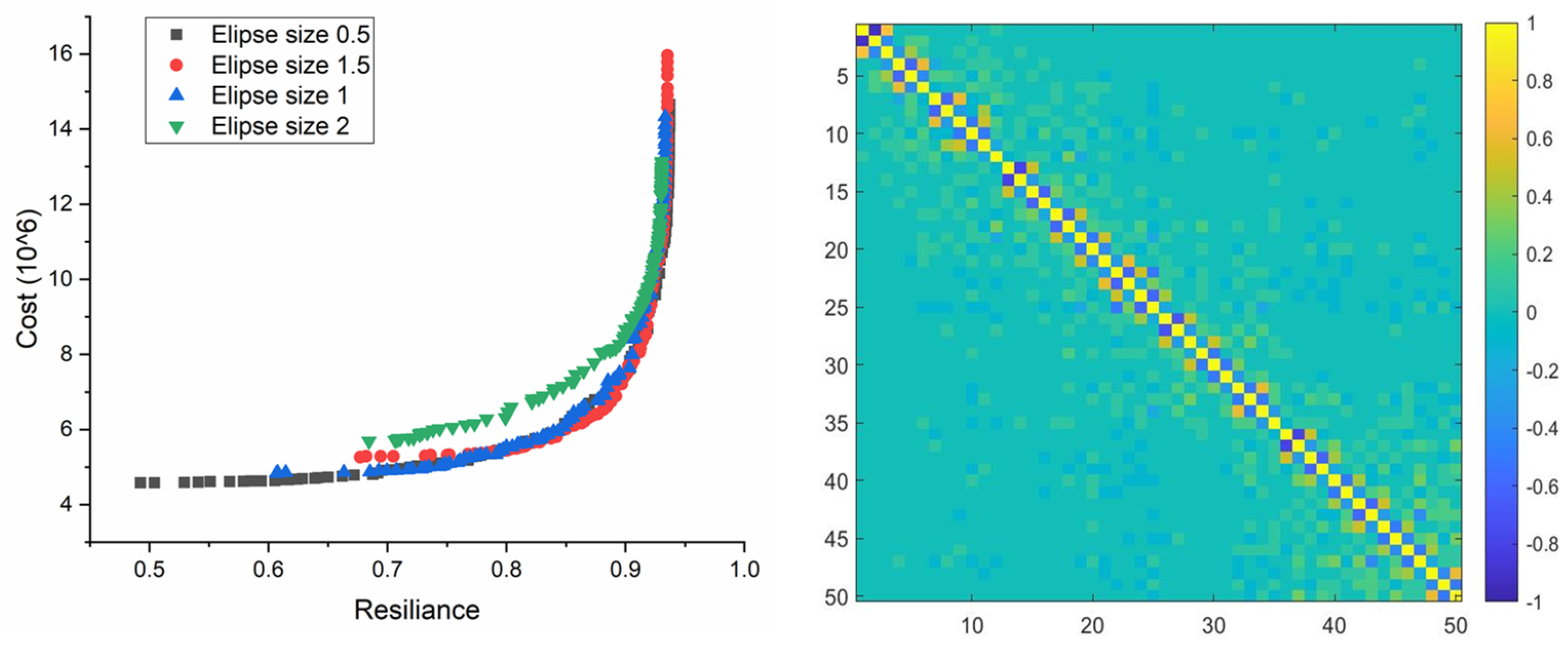
All the demands are considered uncertain, and the mean demands are assumed to be base demands mentioned in Table 9d in Alperovits and Shamir [43]. The input file for this network is attached as supporting material. The standard deviation from the means is assumed to be 20% for each node. The unit cost of the available pipe diameters is shown in Table 3. The co-variance between the demand nodes is assumed to be completely heterogenous. Three different co-variance matrices are evaluated with correlations between −0.3 to 0.8 as shown in Figure 5, Figure 6 and Figure 7.
The design Pareto fronts are obtained for three different sets of correlation matrices with four different protection sizes (theta = 0.5, 1, 1.5, 2). Figure 5, Figure 6 and Figure 7 depicts the various Pareto fronts obtained for corresponding co-variance matrices.
Three different co-variance matrices are defined randomly, the first with more positive correlation, the second with more negative correlation, and third with a random pattern. As the network has higher resilience inherently, the demand uncertainty with varying uncertainty sets did not effect as much as it effected for Hanoi WDS. From all the three cases, we can see that as the design resilience increases, there is no effect of increase in the protection level. This shows that designs with higher resilience can handle demand uncertainty. Most variation is seen only in the low resilience designs, and the variation is similar to the results obtained for Hanoi, in which the increase in the protection level leads to an increase in cost.
4. Conclusions
Multi-objective design of water distribution systems under uncertainty is not much explored especially using non-probabilistic techniques to handle the uncertainty. In the current study, one such methodology is proposed, wherein we employ robust optimization techniques combined with standard multi-objective optimization techniques to solve a WDS design problem with uncertain demands, considering the minimization of cost and maximization of resilience as objectives. The proposed methodology is tested on two case studies of standard WDS benchmark problems. The results show that the effect of uncertainty in demand is higher for networks with inherently low topological resilience compared to higher topological resilience networks. Positively correlated demand patterns require higher cost designs to maintain even low resiliency in the network can be inferred from the Hanoi case study. Application to other larger scaled water distribution systems should be explored in future research for overcoming the expected high computational effort involved in such implementations. The extension of this work to multiple loading conditions including storage is another important future research direction.
Author Contributions
S.P.B.: Conceptualization, methodology, results and paper writing. A.O.: Supervisor, conceptualization, paper revision. All authors have read and agreed to the published version of the manuscript.
Funding
This research was supported by the Israel Science Foundation (Grant No. 555/18).
Data Availability Statement
Data associated with this work will be provided upon request to any of the authors.
Conflicts of Interest
The authors declare no conflict of interest.
References
- Prasad, T.D.; Park, N.-S. Multiobjective Genetic Algorithms for Design of Water Distribution Networks. J. Water Resour. Plan. Manag. 2004, 130, 73–82. [Google Scholar] [CrossRef]
- Farmani, R.; Walters, G.A.; Savic, D.A. Trade-off between Total Cost and Reliability for Anytown Water Distribution Network. J. Water Resour. Plan. Manag. 2005, 131, 161–171. [Google Scholar] [CrossRef]
- Kapelan, Z.; Babayan, A.V.; Savic, D.A.; Walters, G.A.; Khu, S.T. Two new approaches for the stochastic least cost design of water distribution systems. Water Sci. Technol. Water Supply 2004, 4, 355–363. [Google Scholar] [CrossRef]
- Moosavian, N.; Lence, B.J. Nondominated Sorting Differential Evolution Algorithms for Multiobjective Optimization of Water Distribution Systems. J. Water Resour. Plan. Manag. 2017, 143, 04016082. [Google Scholar] [CrossRef]
- Naveen Naidu, M.; Boindala, P.S.; Vasan, A.; Varma, M.R.R. Optimization of Water Distribution Networks Using Cuckoo Search Algorithm; Springer: Singapore, 2020; Volume 949, ISBN 9789811381959. [Google Scholar]
- Ostfeld, A. Uncertainty and Risk Inclusions in Water Distribution Systems Management: Review and Challenges. In Proceedings of the Second International Conference on Vulnerability and Risk Analysis and Management (ICVRAM) and the Sixth International Symposium on Uncertainty, Modeling, and Analysis (ISUMA), Liverpool, UK, 13–16 July 2014; pp. 1980–1985. [Google Scholar]
- Pankaj, B.S.; Naidu, M.N.; Vasan, A.; Varma, M.R. Self-Adaptive Cuckoo Search Algorithm for Optimal Design of Water Distribution Systems. Water Resour. Manag. 2020, 34, 3129–3146. [Google Scholar] [CrossRef]
- Patil, M.B.; Naveen Naidu, M.; Vasan, A.; Varma, M.R.R. Water Distribution System Design Using Multi-Objective Genetic Algorithm with External Archive and Local Search. arXiv 2019, arXiv:1905.08105. [Google Scholar]
- Wang, Q.; Guidolin, M.; Savic, D.; Kapelan, Z. Two-Objective Design of Benchmark Problems of a Water Distribution System via MOEAs: Towards the Best-Known Approximation of the True Pareto Front. J. Water Resour. Plan. Manag. 2014, 141, 04014060. [Google Scholar] [CrossRef] [Green Version]
- Bargiela, A.; Hainsworth, G.D. Pressure and flow uncertainty in water systems. J. Water Resour. Plan. Manag. 1989, 115, 212–229. [Google Scholar] [CrossRef]
- Kretzmann, H.A.; van Zyl, J.E. Stochastic Analysis of Water Distribution Systems. In Critical Transitions in Water and Environmental Resources Management; American Society of Civil Engineers: Reston, VA, USA, 2004; pp. 1–10. [Google Scholar]
- Pasha, M.F.K.; Lansey, K. Effect of parameter uncertainty on water quality predictions in distribution systems-case study. J. Hydroinformatics 2010, 12, 1–21. [Google Scholar] [CrossRef] [Green Version]
- Pasha, M.F.K.; Lansey, K. Analysis of uncertainty on water distribution hydraulics and water quality. In Proceedings of the World Water and Environmental Resources Congress 2005, Anchorage, AL, USA, 15–19 May 2005. [Google Scholar]
- Sumer, D.; Lansey, K. Effect of uncertainty on water distribution system model design decisions. J. Water Resour. Plan. Manag. 2009, 135, 38–47. [Google Scholar] [CrossRef]
- Lansey, K.E.; Duan, N.; Mays, L.W.; Tung, Y. Water Distribution System Design Under Uncertainties. J. Water Resour. Plan. Manag. 1989, 115, 630–645. [Google Scholar] [CrossRef] [Green Version]
- Xu, C.; Goulter, I.C. Reliability-based optimal design of water distribution networks. J. Water Resour. Plan. Manag. 1999, 125, 352–362. [Google Scholar] [CrossRef] [Green Version]
- Babayan, A.V.; Kapelan, Z.S.; Savic, D.A.; Walters, G.A. Comparison of two approaches for the least cost design of water distribution systems under uncertain demands. In Critical Transitions in Water and Environmental Resources Management; American Society of Civil Engineers: Reston, VA, USA, 2004; Volume 38, pp. 1–10. [Google Scholar]
- Babayan, A.V.; Savic, D.A.; Walters, G.A.; Kapelan, Z.S. Robust Least-Cost Design of Water Distribution Networks Using Redundancy and Integration-Based Methodologies. J. Water Resour. Plan. Manag. 2007, 133, 67–77. [Google Scholar] [CrossRef]
- Perelman, L.; Housh, M.; Ostfeld, A. Robust optimization for water distribution systems least cost design. Water Resour. Res. 2013, 49, 6795–6809. [Google Scholar] [CrossRef]
- Perelman, L.; Housh, M.; Ostfeld, A. Least-cost design of water distribution systems under demand uncertainty: The robust counterpart approach. J. Hydroinformatics 2013, 15, 737–750. [Google Scholar] [CrossRef] [Green Version]
- Kapelan, Z.S.; Savic, D.A.; Walters, G.A. Multiobjective design of water distribution systems under uncertainty. Water Resour. Res. 2005, 41, 1–15. [Google Scholar] [CrossRef]
- Giustolisi, O.; Laucelli, D.; Colombo, A.F. Deterministic versus Stochastic Design of Water Distribution Networks. J. Water Resour. Plan. Manag. 2009, 135, 117–127. [Google Scholar] [CrossRef]
- Jung, D.; Kang, D.; Kim, J.H.; Lansey, K. Robustness-Based Design of Water Distribution Systems. J. Water Resour. Plan. Manag. 2014, 140, 04014033. [Google Scholar] [CrossRef]
- Seifollahi-Aghmiuni, S.; Bozorg Haddad, O.; Mariño, M.A. Water Distribution Network Risk Analysis Under Simultaneous Consumption and Roughness Uncertainties. Water Resour. Manag. 2013, 27, 2595–2610. [Google Scholar] [CrossRef]
- Hwang, H.; Lansey, K.; Jung, D. Accuracy of First-Order Second-Moment Approximation for Uncertainty Analysis of Water Distribution Systems. J. Water Resour. Plan. Manag. 2018, 144, 04017087. [Google Scholar] [CrossRef]
- Tolson, B.A.; Maier, H.R.; Simpson, A.R.; Lence, B.J. Genetic Algorithms for Reliability-Based Optimization of Water Distribution Systems. J. Water Resour. Plan. Manag. 2004, 130, 63–72. [Google Scholar] [CrossRef] [Green Version]
- Housh, M.; Ostfeld, A.; Shamir, U. Optimal multiyear management of a water supply system under uncertainty: Robust counterpart approach. Water Resour. Res. 2011, 47, 1–15. [Google Scholar] [CrossRef]
- Matrosov, E.S.; Woods, A.M.; Harou, J.J. Robust Decision Making and Info-Gap Decision Theory for water resource system planning. J. Hydrol. 2013, 494, 43–58. [Google Scholar] [CrossRef]
- Korteling, B.; Dessai, S.; Kapelan, Z. Using Information-Gap Decision Theory for Water Resources Planning Under Severe Uncertainty. Water Resour. Manag. 2013, 27, 1149–1172. [Google Scholar] [CrossRef] [Green Version]
- Pankaj, B.S.; Jaykrishnan, G.; Ostfeld, A. Optimizing Water Quality Treatment Levels for Water Distribution Systems under Mixing Uncertainty at Junctions. J. Water Resour. Plan. Manag. 2022, 148, 04022013. [Google Scholar] [CrossRef]
- Roach, T.; Kapelan, Z.; Ledbetter, R. Comparison of info-gap and robust optimisation methods for integrated water resource management under severe uncertainty. Procedia Eng. 2015, 119, 874–883. [Google Scholar] [CrossRef] [Green Version]
- Schwartz, R.; Housh, M.; Ostfeld, A. Limited multistage stochastic programming for water distribution systems optimal operation. J. Water Resour. Plan. Manag. 2016, 142, 06016003. [Google Scholar] [CrossRef]
- Ben-Tal, A.; Nemirovski, A. Robust Convex Optimization. Math. Oper. Res. 1998, 23, 769–805. [Google Scholar] [CrossRef] [Green Version]
- Engelhardt, M.O.; Skipworth, P.J.; Savic, D.A.; Saul, A.J.; Walters, G.A. Rehabilitation strategies for water distribution networks: A literature review with a UK perspective. Urban Water 2000, 2, 153–170. [Google Scholar] [CrossRef]
- Walski, T.M. The Wrong Paradigm—Why Water Distribution Optimization Doesn’t Work. J. Water Resour. Plan. Manag. 2001, 127, 203–205. [Google Scholar] [CrossRef]
- Fu, G.; Kapelan, Z.; Reed, P. Reducing the Complexity of Multiobjective Water Distribution System Optimization through Global Sensitivity Analysis. J. Water Resour. Plan. Manag. 2012, 138, 196–207. [Google Scholar] [CrossRef]
- Shannon, C.E. A Mathematical Theory of Communication. Bell Syst. Tech. J. 1948, 27, 379–423. [Google Scholar] [CrossRef] [Green Version]
- Todini, E. Looped water distribution networks design using a resilience index based heuristic approach. Urban Water 2000, 2, 115–122. [Google Scholar] [CrossRef]
- Gheisi, A.; Forsyth, M.; Naser, G. Water Distribution Systems Reliability: A Review of Research Literature. J. Water Resour. Plan. Manag. 2016, 142, 04016047. [Google Scholar] [CrossRef]
- Dziedzic, R.; Karney, B.W. Performance Index for Water Distribution Networks under Multiple Loading Conditions. J. Water Resour. Plan. Manag. 2016, 142, 04015040. [Google Scholar] [CrossRef]
- Geem, Z.W. Multiobjective optimization of water distribution networks using fuzzy theory and harmony search. Water (Switzerland) 2015, 7, 3613–3625. [Google Scholar] [CrossRef]
- Fujiwara, O.; Khang, D.B. A two-phase decomposition method for optimal design of looped water distribution networks. Water Resour. Res. 1990, 26, 539–549. [Google Scholar] [CrossRef]
- Alperovits, E.; Shamir, U. Design of optimal water distribution systems. Water Resour. Res. 1977, 13, 885–900. [Google Scholar] [CrossRef]
- Design/Resiliance | Engineering | University of Exeter. Available online: https://emps.exeter.ac.uk/engineering/research/cws/resources/benchmarks/design-resiliance-pareto-fronts/ (accessed on 30 June 2022).
Figure 1.
Flow chart of self-adaptive multi-objective Cuckoo search algorithm (SAMOCSA).

Figure 2.
Graphical representation of Hanoi WDS with junctions as nodes and pipes as links.

Figure 3.
(a) Graph showing the WDS design Pareto fronts for Hanoi WDS with demand variation with positive correlation; (b) graph showing the WDS design Pareto fronts for Hanoi WDS with demand variation with negative correlation; (c) graph showing the WDS design Pareto fronts for Hanoi WDS with demand variation with no correlation.


Figure 4.
Graphical representation of large network introduced by Alperovits and Shamir.

Figure 5.
Pareto front obtained for different ellipsoidal sizes with demands related with co-variance matrix (1) shown adjacent.
Figure 5.
Pareto front obtained for different ellipsoidal sizes with demands related with co-variance matrix (1) shown adjacent.

Figure 6.
Pareto front obtained for different ellipsoidal sizes with demands related with co-variance matrix (2) shown adjacent.
Figure 6.
Pareto front obtained for different ellipsoidal sizes with demands related with co-variance matrix (2) shown adjacent.

Figure 7.
Pareto front obtained for different ellipsoidal sizes with demands related with co-variance matrix (3) shown adjacent.
Figure 7.
Pareto front obtained for different ellipsoidal sizes with demands related with co-variance matrix (3) shown adjacent.


Table 1.
List of few works in the area so WDS design and analysis under uncertainty.
| Uncertain Parameters | PDF Assumed | Uncertainty Handling Techniques | Optimization Techniques | References | Type |
|---|---|---|---|---|---|
| q, H, RC | Normal | FORM | GRG2 | [16] | Hydraulic analysis |
| q, H, RC | Normal | MCS | GRG2 | [15] | SO Design |
| q, RC | Normal | MCS | SFLA | [24] | Hydraulic analysis |
| q, RC | Normal | FOSM and MCS | -- | [25] | Hydraulic analysis |
| q | Gaussian | LHS | GA | [17] | SO Design |
| q, RC | Normal | FORM | GA | [26] | SO Design |
| q | Gaussian | LHS | RNSGA-II | [21] | MO Design |
| q | -- | Robust optimization | cross entropy | [19,20] | SO Design |
Note(s): q—demand; RC—roughness coefficient; H—pressure head; LHS—Latin hypercube sampling; MCS—Monte Carlo simulations; GA—genetic algorithm; FORM—first-order reliability method; SO—single objective; MO—multi-objective design; SFLA—shuffled frog leap algorithm.
Table 2.
Diameter options and associated unit costs for Hanoi WDS.
| Diameter (in) | Unit Cost ($/m) | Diameter (in) | Unit Cost ($/m) | Diameter (in) | Unit Cost ($/m) |
|---|---|---|---|---|---|
| 12.0 | 45.73 | 20 | 98.39 | 30 | 180.75 |
| 16.0 | 70.4 | 24 | 129.33 | 40 | 278.28 |
Table 3.
Cost and resilience comparison of extreme points in the Pareto front for two different uncertainty set sizes.
Table 3.
Cost and resilience comparison of extreme points in the Pareto front for two different uncertainty set sizes.
| Correlation | Uncertainty Set Size | Extreme Point-1 | Extreme Point-2 | ||
|---|---|---|---|---|---|
| Cost | Resilience | Cost | Resilience | ||
| Positive | 2 | 7.9157 | 0.154 | 10.969 | 0.186 |
| 0.5 | 6.7115 | 0.2394 | 10.755 | 0.3118 | |
| Negative | 2 | 7.154 | 0.207 | 10.121 | 0.2593 |
| 0.5 | 6.61 | 0.2516 | 10.305 | 0.3298 | |
| Zero(No) | 2 | 6.656 | 0.2211 | 10.747 | 0.308 |
| 0.5 | 6.584 | 0.2232 | 10.769 | 0.342 | |
Table 4.
Diameter options and associated unit costs for large network.
| Diameter | 1 | 2 | 3 | 4 | 6 | 8 | 10 | 12 | 14 | 16 | 18 | 20 |
| Unit Cost | 2.0 | 5.0 | 8.0 | 11.0 | 16.0 | 24.0 | 32.0 | 50.0 | 60.0 | 90.0 | 130.0 | 170.0 |
Publisher’s Note: MDPI stays neutral with regard to jurisdictional claims in published maps and institutional affiliations. |
© 2022 by the authors. Licensee MDPI, Basel, Switzerland. This article is an open access article distributed under the terms and conditions of the Creative Commons Attribution (CC BY) license (https://creativecommons.org/licenses/by/4.0/).
Share and Cite
MDPI and ACS Style
Boindala, S.P.; Ostfeld, A. Robust Multi-Objective Design Optimization of Water Distribution System under Uncertainty. Water 2022, 14, 2199. https://doi.org/10.3390/w14142199
AMA Style
Boindala SP, Ostfeld A. Robust Multi-Objective Design Optimization of Water Distribution System under Uncertainty. Water. 2022; 14(14):2199. https://doi.org/10.3390/w14142199
Chicago/Turabian StyleBoindala, Sriman Pankaj, and Avi Ostfeld. 2022. "Robust Multi-Objective Design Optimization of Water Distribution System under Uncertainty" Water 14, no. 14: 2199. https://doi.org/10.3390/w14142199
Note that from the first issue of 2016, this journal uses article numbers instead of page numbers. See further details here.