Article

Curating 62 Years of Walnut Gulch Experimental Watershed Data: Improving the Quality of Long-Term Rainfall and Runoff Datasets

by
Menberu B. Meles
1,2,3,*,
Eleonora M. C. Demaria
1,
Philip Heilman
1,
David C. Goodrich
1,
Mark A. Kautz
1,
Gerardo Armendariz
1,
Carl Unkrich
1,
Haiyan Wei
2 and
Anandraj Thiyagaraja Perumal
1
1
USDA-ARS, Southwest Watershed Research Center, Tucson, AZ 85719, USA
2
School of Natural Resources and the Environment, University of Arizona, Tucson, AZ 85721, USA
3
USDA-ARS, Sustainable Agricultural Water Systems Research, Davis, CA 95616, USA
*
Author to whom correspondence should be addressed.
Water 2022, 14(14), 2198; https://doi.org/10.3390/w14142198
Submission received: 20 May 2022 / Revised: 29 June 2022 / Accepted: 30 June 2022 / Published: 12 July 2022
(This article belongs to the Special Issue Data Handling and Mining for Water Resources Planning and Management)

Abstract

:
The curation of hydrologic data includes quality control, documentation, database development, and provisions for public access. This article describes the development of new quality control procedures for experimental watersheds like the Walnut Gulch Experimental Watersheds (WGEW). WGEW is a 149 km2 watershed outdoor hydrologic laboratory equipped with a dense network of hydro-climatic instruments since the 1950s. To improve data accuracy from the constantly growing instrumentation networks in numerous experimental watersheds, we developed five new QAQC tools based on fundamental hydrologic principles. The tools include visual analysis of interpolated rainfall maps and evaluating temporal, spatial, and quantitative relationships between paired rainfall-runoff events, including runoff lag time, runoff coefficients, multiple regression, and association methods. The methods identified questionable rainfall and runoff observations in the WGEW database that were not usually captured by the existing QAQC procedures. The new tools were evaluated and confirmed using existing metadata, paper charts, and graphical visualization tools. It was found that 13% of the days (n = 780) with rainfall and 7% of the runoff events sampled had errors. Omitting these events improved the quality and reliability of the WGEW dataset for hydrologic modeling and analyses. This indicated the effectiveness of application of conventional hydrologic relations to improve the QAQC strategy for experimental watershed datasets.

1. Introduction

Long-term observations are the foundation for understanding earth system processes for sustainable water and natural resource management under current and future climate conditions [1]. As the uncertainty in water supply increases with warmer temperatures and a growing human population, the need for high quality, long-term hydrometeorological observations to facilitate sustainable use, management, and scientific research at a regional scale and beyond has increased. Data collected in experimental watersheds and natural research observatories across the U.S., such as the United States Department of Agriculture—Agricultural Research Service (USDA-ARS) Long-Term Agroecosystem Research (LTAR) network [2,3,4], the Critical Zone Observatories (CZO) [5], the Long-term Ecological Research (LTER) network [6], and the National Ecological Observatory Network (NEON) sites [7] are critical for research, analyses and planning [1]. However, these observations must be continually monitored for errors to improve the knowledge about the quality and limitations of the datasets, which are often inevitably inadequate, e.g., [8], and to make the data accessible to the growing base of scientists and stakeholders.
Measurements and modeling have gone hand-in-hand since before hydrology began as a formal science [9]. Hydrological analysis for sustainable and resilient engineering designs and modeling hydrological systems for understanding changes and management strategies have been the center of hydrological research over the years, e.g., [10,11,12,13]. Especially at large spatial domains, hydrologic modeling and analysis are severely constrained by data availability and data quality limiting our ability to provide accurate predictions and inferences, e.g., [14,15,16,17,18]. Ensuring the accuracy of datasets for scientific analysis requires a large investment of time and money. Furthermore, these efforts need to be operationally feasible. Errors in the magnitude of observations such as total volume/peak runoff, total rainfall, or their associated timestamp will create physically unrealistic rainfall-runoff relations making the data unsuitable for modeling or other hydrologic analyses. From an ecosystem analysis standpoint, errors in rainfall or runoff observations can lead to inconsistencies in model parameterization and predictions, errors in water balance partitioning, and erroneous hydroclimatic analyses. In the past, hydrologic relations such as the use of recession curves to identify inconsistencies, e.g., [18,19], out of range runoff coefficients, and other temporal water balance analyses [8,20] were widely used. The application of real-time special consistency analysis on personal weather stations (PWS) without the need for auxiliary instruments [21] was recently used to improve hydrologic data analysis. Common methods to ensure the integrity of data, referred to as quality assurance and quality control (QAQC) procedures, include outlier checks using a threshold value [22], fitting to theoretical probability distribution functions to flag outliers, comparisons with neighboring stations, use of duplicate sensors [4,23,24,25,26] and evaluation of rating curves which became obsolete due to changes in the channel morphology, e.g., [9]. QAQC procedures result in improvements to the quality of a dataset through a combination of steps. This includes preventing errors from occurring through improved data collection and management practices (quality assurance, QA), and the identification and resolution of errors within the recorded dataset (quality control, QC). QC efforts have historically been performed on rainfall and runoff observations independently; however, given the causality between the measurements, a new QC procedure was developed that considered the relationships between rainfall and runoff to potentially identify more errors that may not be identified by other conventional methods to improve the overall quality of the dataset further.
The USDA-ARS is responsible for assessing the quality of and curating large biophysical datasets for numerous experimental watersheds and research networks and for delivery of the datasets to the public. Scientists at the USDA-ARS Southwest Watershed Research Center (SWRC) have been collecting biophysical data at the Walnut Gulch Experimental Watershed (WGEW) near Tombstone, Arizona, for more than 60 years. During that time, SWRC scientists and staff have consistently advanced QA procedures to ensure the WGEW database is accurate and error-free for all biophysical variables measured in the watershed. This continues to be a focus of SWRC scientists as the observational period of record grows in length under a changing climate and an expansion of research needs leads to collection of additional types of data.
WGEW is an LTAR network site with commitments to long-term sustainable research [2]. The WGEW was established in order to better understand rainfall-runoff relationships and soil loss within semiarid, ephemeral catchments that are prone to flash flooding during summertime convective rainfall events [27,28,29]. Measurements of runoff, water yield, and sediment loss were paired with precipitation measurements to begin to address the initial research questions at WGEW. These measurements have grown to include vegetation, geomorphology, land-atmosphere fluxes, meteorology, and other observations to facilitate the evolving research program and diverse needs of the SWRC and its collaborators. WGEW observations, past and current, are essential datasets to address the wide range of objectives related to arid and semi-arid systems.
WGEW data measurements have been the foundation of several impactful research and technology developments that have advanced the hydrological sciences and engineering for arid and semiarid watersheds. Thus far, these data have resulted in over 2000 publications, listed in the USDA-ARS-Southwest Watershed Research Center publication database (https://www.tucson.ars.ag.gov/unit/Publications/Search.html, accessed on 1 May 2022), which required quality data as accurate and error-free as possible. The SWRC has also adapted to the changing spatial and temporal demands of evolving research needs, which include long-term land use and climatic change expanding to multi-site studies through research networks like LTAR and NEON [28,29,30]. To these effects, the SWRC has invested considerable resources in both QA, through regular sensor calibrations, site maintenance, installation of consistent instrumentation across networks, testing of new instrumentation prior to adoption, and installation of redundant sensors to compare observations, e.g., [31], and QC through regular data inspection and analysis conducted by SWRC scientists and technicians.
QAQC procedures at WGEW have evolved to accommodate the observations made by the now retired analog instrumentation [32] and current digital instrumentation [33]. The long-term record of measurements from the WGEW is archived in the Data Access Project (DAP—https://www.tucson.ars.ag.gov/dap/, accessed on 1 May 2022) database, which was initiated in the year 2000 following the replacement of analog instrumentation by digital instruments [34]. Although rainfall and runoff observations from the WGEW are routinely checked for inconsistencies and errors using the existing QAQC procedures, some errors remain in the data. Most errors are due to problems associated with analog clocks used before 2000 that required comprehensive tools to auto-flag erroneous data.
The goal of the study was to develop and evaluate new QAQC procedures for WGEW database based on fundamental hydrologic principles for evaluating and maintaining the quality of experimental watersheds’ datasets. The objectives of the study included (1) identifying, verifying, and removing or correcting the inconsistent rainfall and runoff observations in WGEW and (2) assessing the impacts of QC and the challenges of rainfall-runoff process reproducibility using the flagged datasets in Walnut Gulch. The methodologies developed and applied in this study are aimed at improving the quality and integrity of data for Walnut Gulch but are applicable for large datasets from experimental watersheds elsewhere. The need for such tools is growing commensurate with the increasing number of large collaborative research networks (LTAR, CZO, etc.) and respective data provisioning.

2. Data Description and Quality Control Methodology

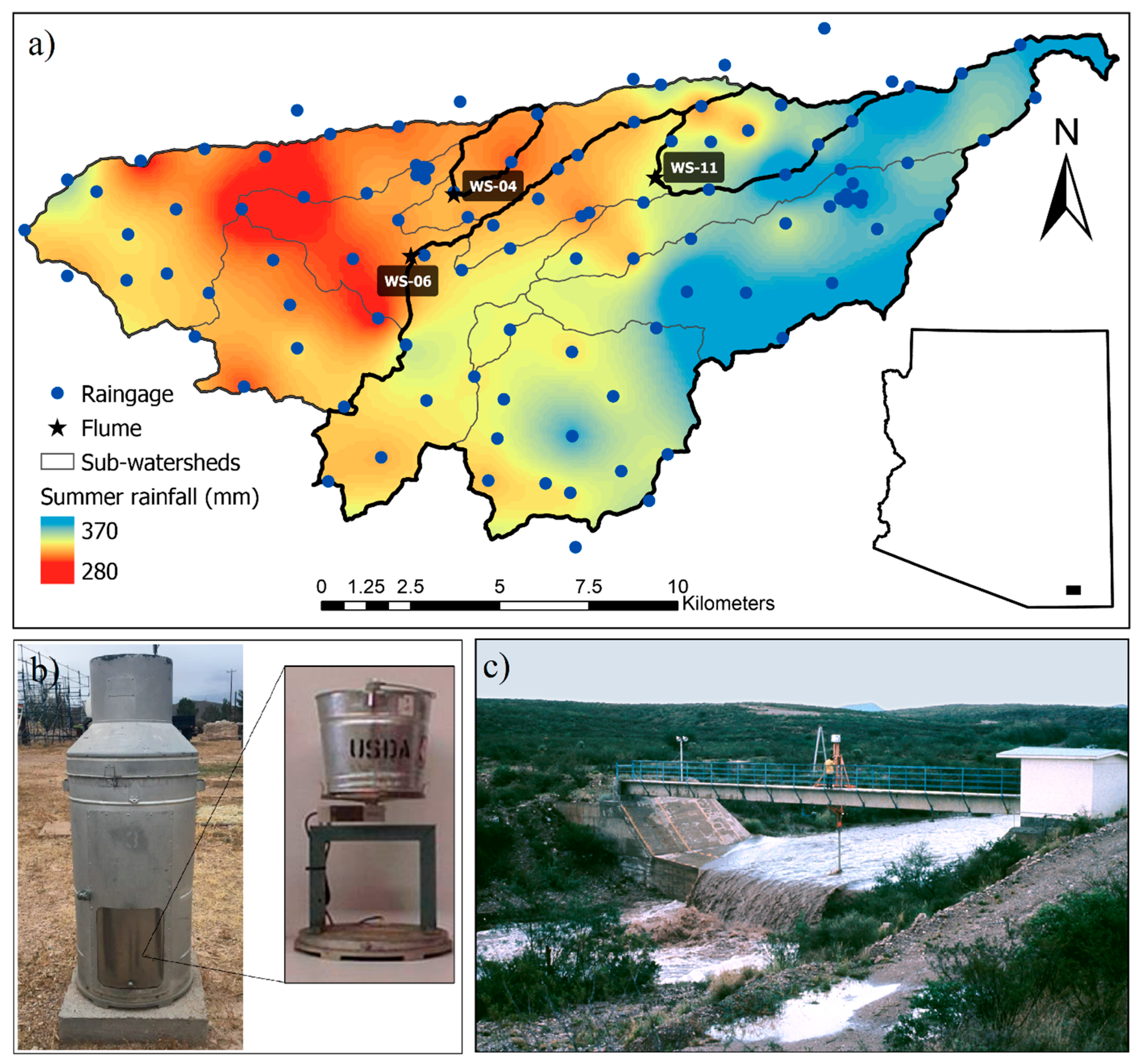
2.1. WGEW Data and Site Description

The WGEW (Figure 1a) was established by the USDA-ARS-SWRC in southeastern Arizona during the 1950s and has been in continuous operation since that time [33,35]. Average summer (May through September) rainfall, over the entire watershed for the 1961–2017 period, is approximately 293 mm (112 to 370 mm range) with~60% falling during summer monsoon [36]. Summer rainfall at WGEW typically occurs as intense, short duration, localized, spatially isolated thunderstorms characteristic of the North American Monsoon (NAM) [37,38]. To accurately measure and understand the complex processes resulting from spatially isolated thunderstorms and the resulting runoff during the summer season, WGEW is equipped with a dense network of rain gauges and runoff measurement structures. Based on experience from eastern and mid-western watersheds, 20 rain gauges were initially installed across the WGEW. This increased to 99 rain gauges over time to capture the high spatiotemporal variability of rainfall generated from thunderstorms during the summer NAM season [39]. Rain gauge density per area is approximately one gauge per 1.7 km2, making WGEW the densest rainfall network on a semiarid experimental watershed in the world [40,41]. Since the establishment of ARS experimental watersheds in other regions of the country starting in the mid-1930s, the primary precipitation gauges employed have been a Belfort 8-inch (0.2032 m) unshielded weighing-bucket gauge (Figure 1b), with a resolution of 0.01 inches (0.254 mm). With evolving digital technology, in the mid-1990s, the Belfort rain gauges were replaced with weighing gauges utilizing a strain gauge and a digital datalogger.
There is a total of 18 nested sub-watersheds within WGEW using v-notch weirs, H flumes, and supercritical flumes designed for the Walnut Gulch channel environment [42,43] (see. Figure 1c for supercritical flume photo) fitted with analog recorders. After 2000, potentiometers connected to data loggers were installed on the runoff stage recorders. This eliminated the labor-intensive weekly visits to wind clocks, change recording pens, and change charts. The WGEW watershed is also equipped with three meteorological stations, two eddy covariance flux towers, several soil moisture sensors at various depths, and eight gauged stock tanks/ponds [43,44]. In addition to the hydrologic observations, climate, and sediment, the SWRC has extensive datasets related to vegetation abundance and diversity and conducted extensive research in geology, soils, ecology, and range management, which provide a broad set of data and proxies to investigate changes in water resources. All WGEW data (current and historical) are available through the web-based portal (https://www.tucson.ars.ag.gov/dap/, accessed on 1 May 2022). The current study utilizes data across the entire watershed and includes focused analyses on rainfall and runoff data from three main sub-watersheds within WGEW: WS-04, WS-011, and WS-06 (Figure 1a), with contributing areas of 2.3, 8.2, and 95.1 km2, respectively. In the sub-watersheds, there are 5, 12, and 56 rain gauges, respectively. The outlets of the sub-watersheds are instrumented with supercritical flume structures, with each typically recording 3–8 runoff events per year. Almost 100% of the runoff is during the summer monsoon seasons, so the limited number of runoff events generated per year on each sub-watershed necessitates capturing each event accurately.
Rainfall and runoff observations have been archived in both paper and digital formats at sub-hourly frequency using breakpoint format, which consists of the times of change from one steady rate to another with a minimum time step of 1 min. In the breakpoint data, the data pairs consist of time and rainfall or runoff depth with zero values at the beginning and end of the event recordings. A direct, side-by-side comparison of events before and after the change from analog to digital gauges using co-located analog/digital rain gauges was conducted for a 5-year period for nine rain gauges from 2000–2004. This analysis concluded that no measurement discontinuities in raw and derived quantities (e.g., peak 30 min rainfall intensity) were introduced by the switch in the weighing and recording systems [45]. In preparation for the current study, however, we observed that the data from the analog period contained more errors than data from the digital period, which was largely attributed to mechanical clocks slowing down, speeding up, or stopping between visits, as well as expansion or contraction of paper charts, and the manual digitizing process.

2.2. Past and Present QAQC Processes

Substantial effort has been invested over the years to ensure the quality of the WGEW rainfall and runoff data [32,40]. For QA, rain gauges and flume installations are regularly inspected for electro-mechanical problems and potential environmental interference (like overgrown vegetation or damage from wildlife) and are calibrated annually prior to the monsoon season. For QC of data from the analog instrumentation, there were a number of steps after the paper charts were collected from the rain gauges and flumes. For rainfall, much of the work was devoted to identifying the days on which the rainfall occurred. Because most rain gauges had charts on drums that completed one rotation every 24 h, and the charts were collected weekly, there were 7 days of pen lines overlaid across each chart. This was partly mitigated by a handful of gauges across the watershed that were re-geared to rotate once per week. The charts were manually digitized, using technologies ranging from visually reading the charts, to an electro-mechanical digitizer connected to a keypunch machine, to a modern digitizing tablet connected to a computer. Review and correction to runoff data was usually done before digitizing, whereas correction to rainfall data was done primarily after digitizing. The main QC tool for rainfall was a computer program that produced crude printed maps showing categorized rainfall amounts or event starting times across the watershed. Large discrepancies between adjacent gauges were flagged for further investigation. This program was later upgraded to a graphical user interface that also included rainfall hyetographs.
Currently, the workflow from field measurement to storage in the database and public access through the web-interface includes several steps. The raw data and summary reports are transmitted to a central location daily and are internally accessible for monitoring, identifying malfunctions, and deploying maintenance technicians. The data undergoes a QC process by a trained technician every 2–3 weeks, which includes visual inspection of the hyetographs, hydrographs [4,23], and maps of daily rainfall. Using these procedures, most errors are identified. However, given the harsh environmental conditions, technician errors, and operational changes, maintaining data quality remains challenging. Furthermore, the continually growing number of instruments and the diversity of measurements makes this effort increasingly burdensome.
Data errors generally fall into five categories: instrument malfunctions, field technician errors, transmission errors, data processing errors, and documentation errors. The vast majority of instrument malfunctions were due to the mechanical clocks in the analog instrumentation, but errors due to wind, animals, and vandalism are also seen. Examples of errors by field technicians include writing an incorrect time or date on a chart or failing to toggle a maintenance switch when servicing a digital instrument. There were occasional transcription errors or omissions when processing the analog data, not surprising given the large volume of charts. A documentation error is an omission in the operational status of an instrument. WGEW data is event-based, as opposed to a continuous time series, so the absence of data implies zero values, and there are no “no data” values. Therefore, the user must consult external documentation (metadata) to determine if the instrument was offline at any time during the period of interest.

2.3. Methods

Three new QAQC procedures that exploit the causality and association between rainfall and runoff to augment the currently implemented procedures are presented in the following section. These procedures are based on fundamental hydrologic principles related to this ephemeral system and include five new tools for identifying potentially erroneous rainfall and runoff events. Furthermore, in developing these tools, objective operational bounds for these procedures were quantified. After identifying potentially erroneous events, we evaluated the accuracy of the procedures. These procedures are:
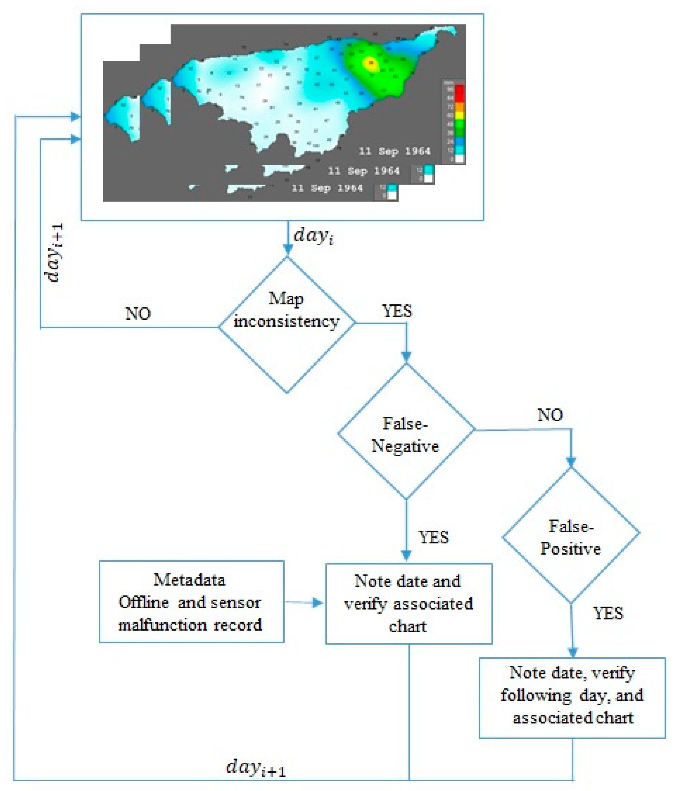
  • Visual inspection of spatial patterns of rainfall;
  • Evaluation of the temporal relationships between rainfall and runoff events:
  • Analysis of the relationship between the amount of rainfall and the amount of runoff.
Visual inspection of spatial patterns of rainfall: WGEW is uniquely equipped to measure rainfall at a high spatial resolution (one gauge per 1.6 km2), which allows for accurate representation of the summer thunderstorms typical of the region [45,46]. Rainfall measurements at adjacent rain gauges show strong spatial correlation, but Keefer et al. (2015) [38] found that correlation of storm totals decreases rapidly as the gauge separation distance increases beyond roughly 2 km. Additionally, [47] also showed the likelihood of independent storms when the spatial correlation falls below 0.27, equivalent to a separation distance greater than 8–8.5 km. This correlation was the basis for the QC method described earlier, using maps of rainfall depths and starting times to identify possible errors. While this procedure has been used as part of the data processing workflow, it has not been used retrospectively to check for errors that might have been missed.
Evaluation of temporal relationships between rainfall and runoff events: Within this ephemeral stream system, there is a direct relation between rainfall and runoff, as base flow is rare. The temporal correlation between rainfall and runoff is complex and influenced by watershed and channel properties, the spatial distribution of rainfall, and antecedent soil moisture conditions. However, one can exploit the basic relationships between rainfall and runoff at a broad level for QC purposes. For instance, runoff cannot exist without rainfall, and there are limits on how far apart these recorded events can be in time. Based on this, two methods were developed:
(1)
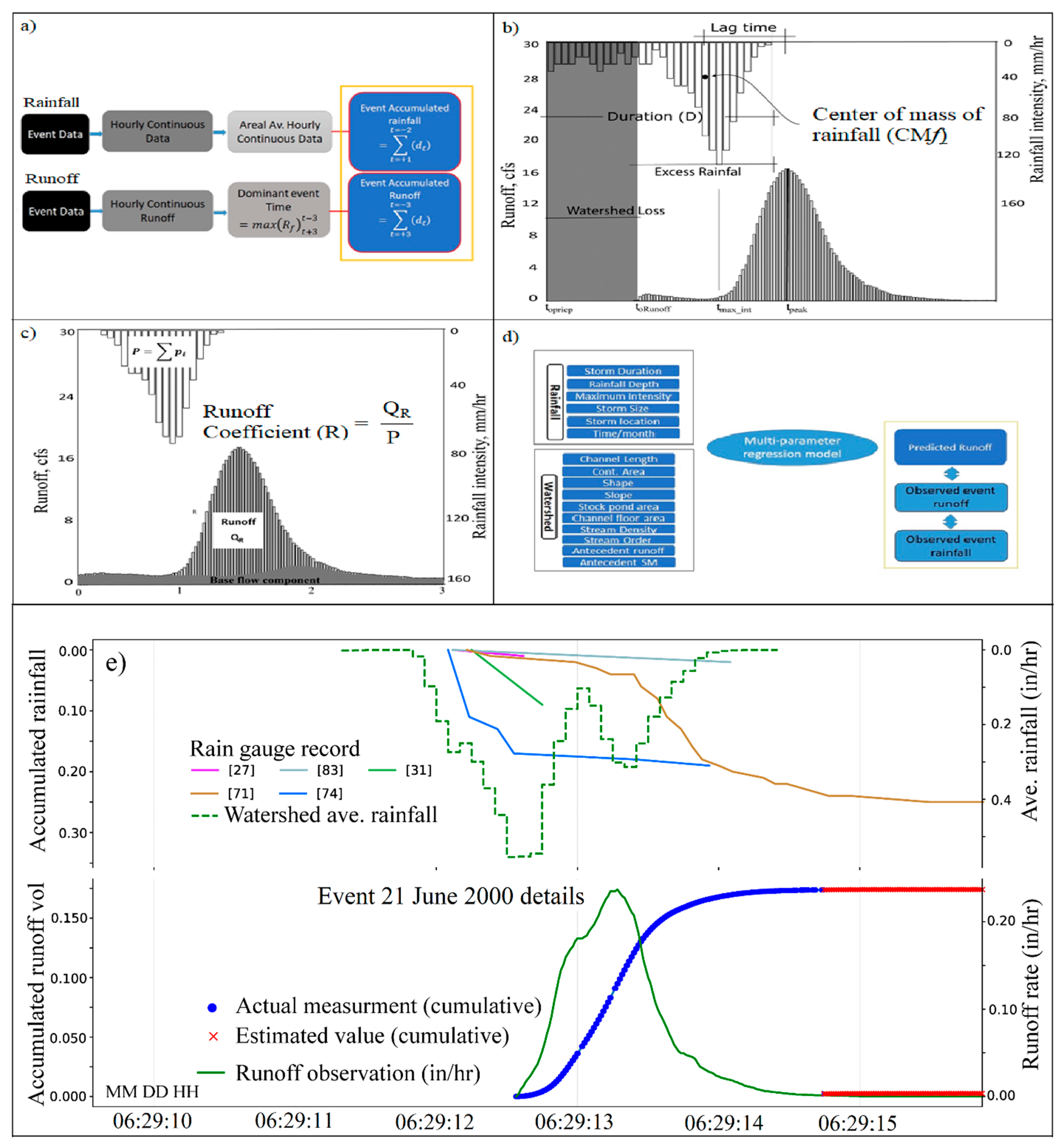
Rainfall-runoff association method: A one-to-one association of rainfall and runoff events in which we evaluate the amount of rain observed within a given window of time for each runoff event. If there is no associated rainfall with the runoff event, it is flagged for further consideration.
(2)
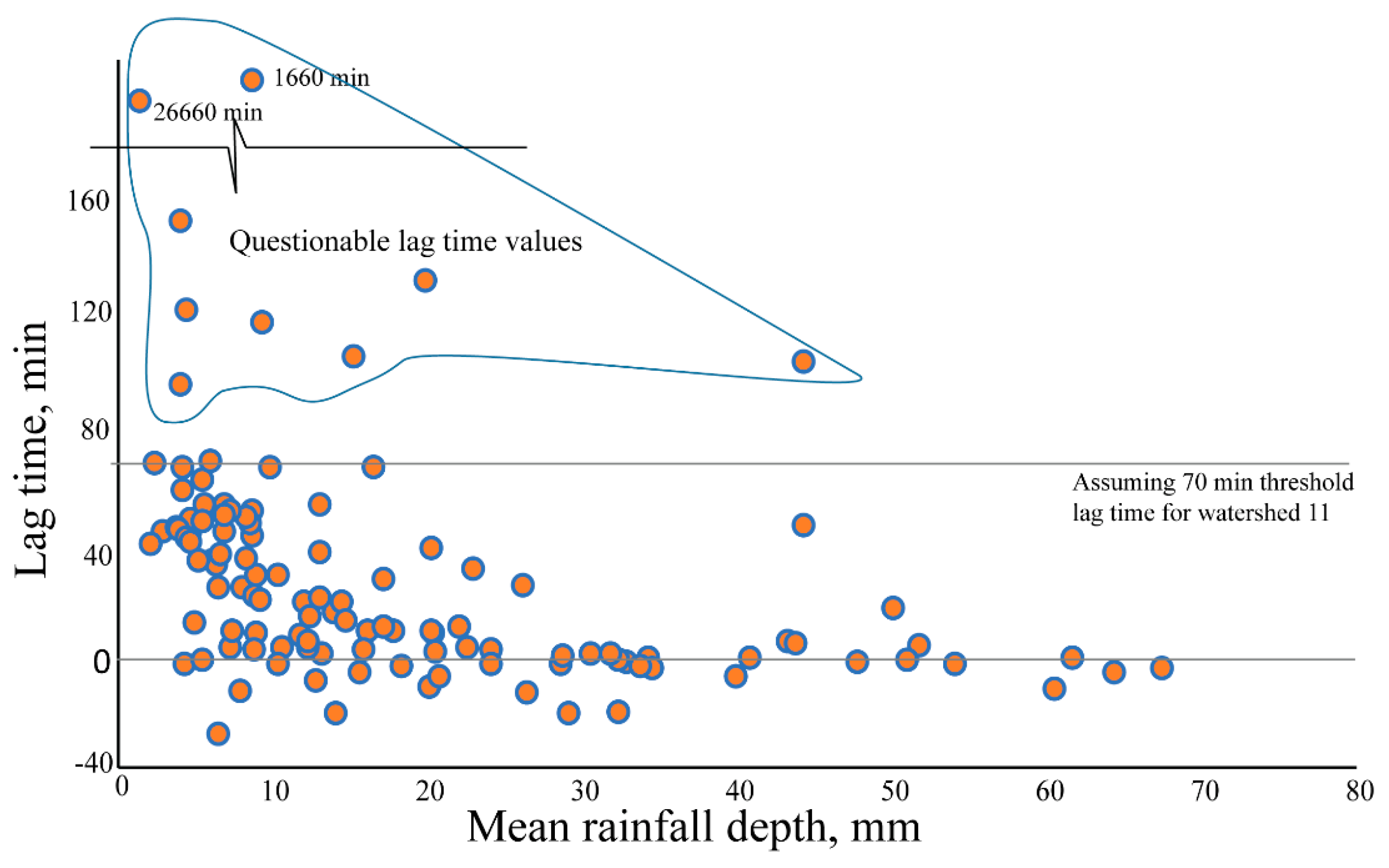
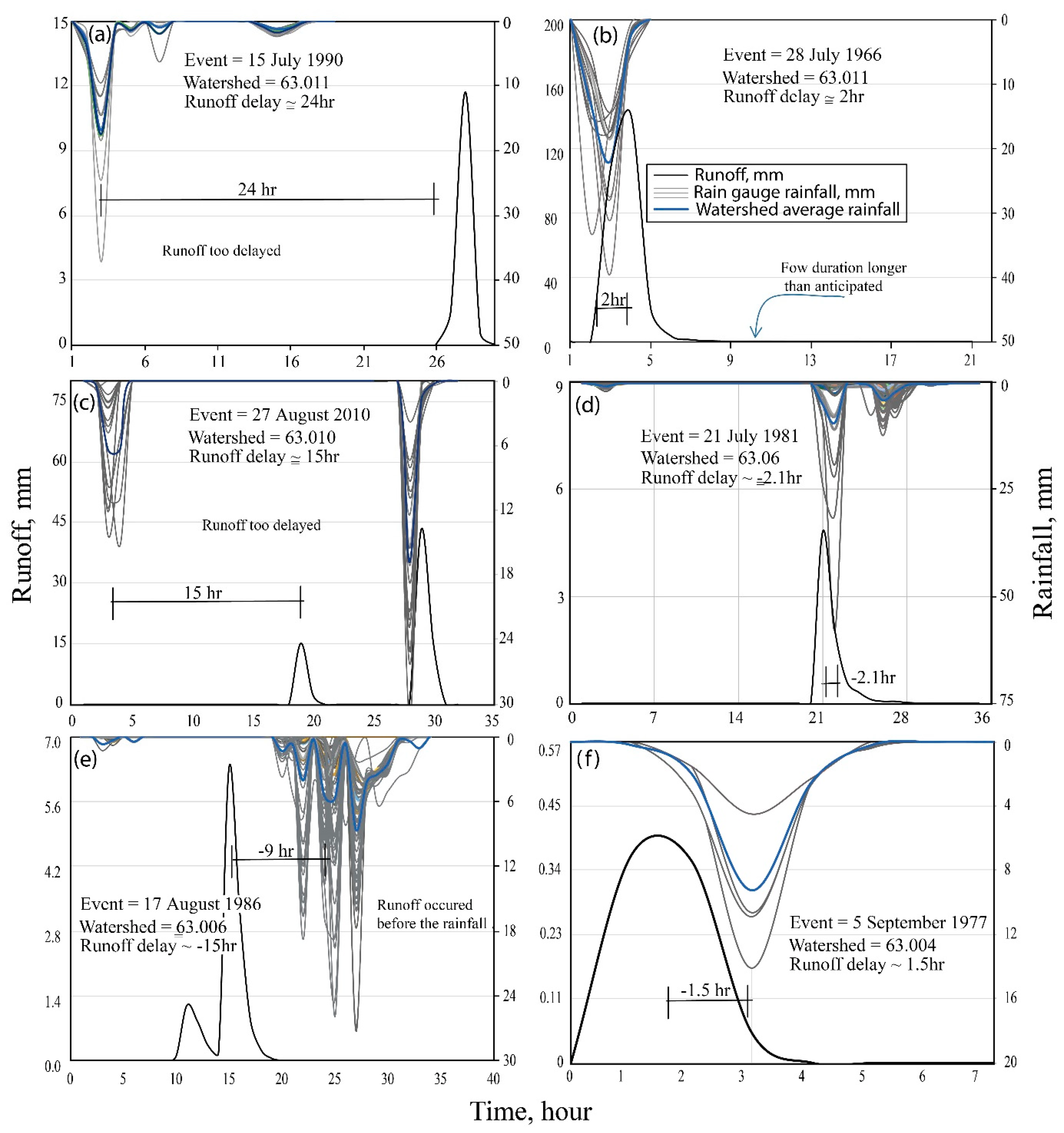
Lag time method: There is certain amount of time that rainfall on a watershed takes to reach the outlet. Computing the value of the delay time between the runoff and the time of precipitation occurrence (lag time) allows us to evaluate if this time is physically realistic. The runoff leaving the outlet should not be too early (e.g., runoff before the rainfall starts) or too late (more than 2 h for medium sized watersheds in Walnut Gulch).
Analysis of relationships between the amount of rainfall and runoff events: Not all rainfall is converted into runoff at WGEW. Runoff is highly dependent on the spatial extent and intensity of rainfall [48,49,50,51]. Moreover, the complex geology, with thick sand deposition in the ephemeral channels and highly conductive hillslopes, results in a highly nonlinear rainfall-runoff relationship [39,52,53]. All or a portion of the rainfall is usually stored the landscape (and eventually returned to the atmosphere) resulting in a runoff to rainfall ratio smaller than one. Losses can occur from infiltration into the upland hillslopes and into the streams via channel transmission losses [39]. These losses are usually large in arid and semiarid regions (>97% in WGEW), resulting in only a small portion of the rainfall converted into runoff; less than 10 mm/year in the driest region of the USA [30]. Given these losses, there are limits to how much runoff can be produced from a rainfall event. The limits depend on rainfall attributes (spatial extent, depth, intensity, duration, etc.) and watershed properties, including extent of ephemeral channels, ground cover, soil, slope shape, etc. While these losses can be very complex, the following tests serve to exploit these relationships for operational QAQC purposes:
(1)
Runoff coefficient method: The runoff coefficient (depth of rainfall divided by the depth of runoff across the watershed) is the metric used in this test to identify runoff events that are physically unrealistic. Specifically, runoff events that are unrealistically large (ratio approaching a value of one (RC)) or associated with no rainfall (infinite value). Runoff coefficients approaching zero are not considered here due to measurement sensitivity/threshold issues at the low end.
(2)
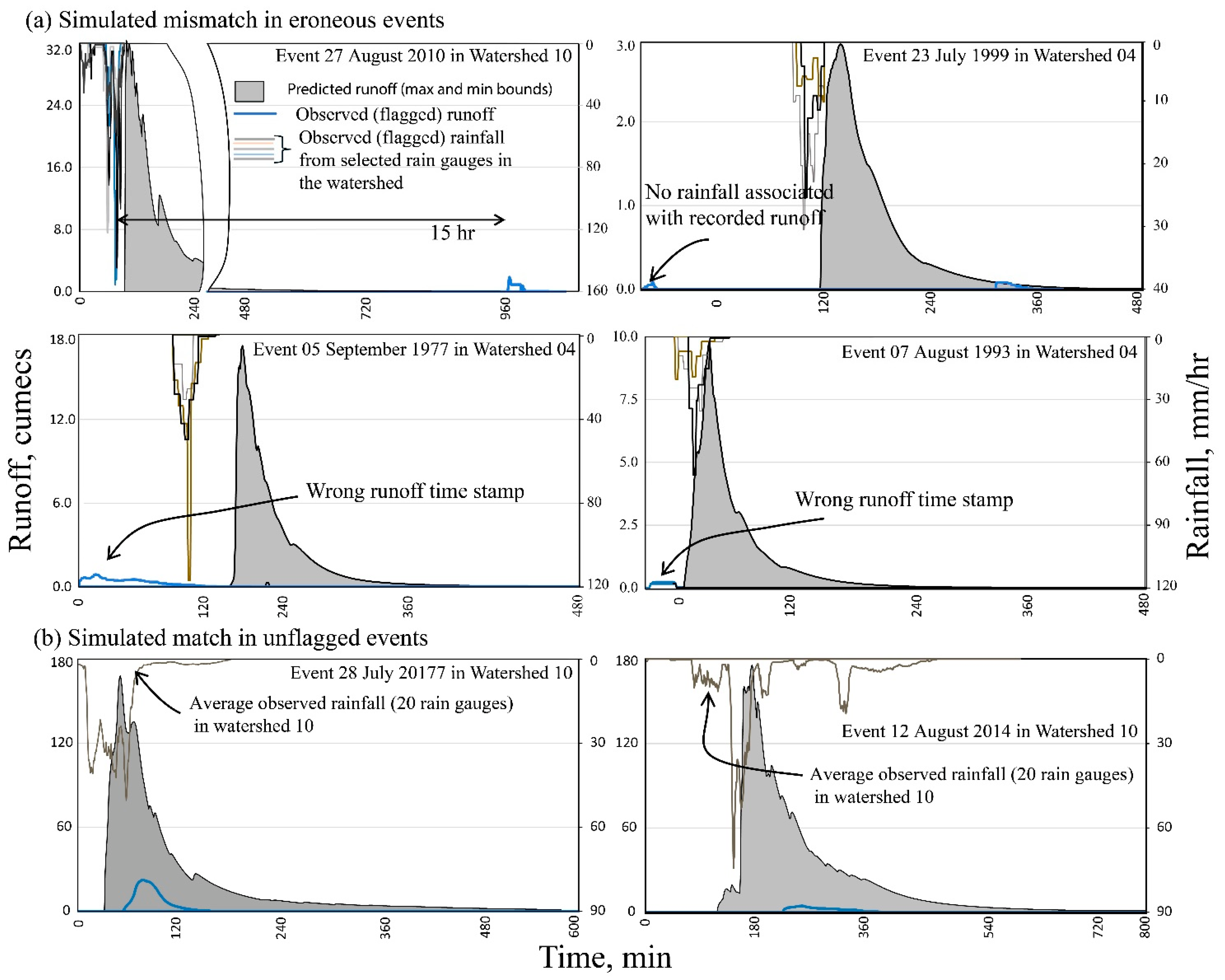
Regression method: This test uses a rainfall-runoff regression model, fully outlined in Bitew et al., 2019 [54], to evaluate the temporal relationships between runoff and precipitation and incorporate watershed properties and antecedent conditions specific to the runoff event and watershed. This method flags suspicious events through comparison between predicted runoff, observed runoff, and the input precipitation.

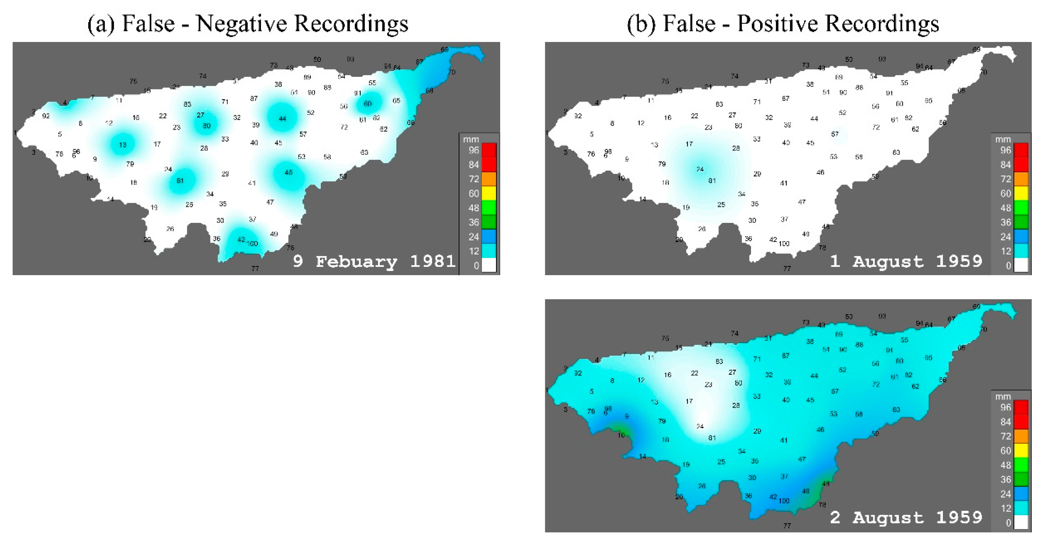
2.3.1. Visual Inspection of Spatial Patterns of Rainfall

Maps of interpolated daily rainfall data across the WGEW were produced for the period 1954–2014. The maps were based on data from 99 rain gauges interpolated at 100 m by 100 m grid spacing using Multiquadric-Biharmonic (MQ-B) interpolation, as described in Garcia et al., (2008) [41] and Houser et al., (2000) [55]. Input to the interpolation program included metadata on gauge installation dates and operational status. If a gauge did not exist or was offline on a given day, it was not included in the interpolation. The gridded data files were then rendered as color maps, with consistent color ramps (Figure 2), which shows either expected rainfall field across the watershed without an error or inconsistent maps with abrupt changes in the rainfall fields. In reviewing the rainfall maps, we identified two types of errors: (1) False-Negative recordings: the result of rain gauges being offline without any corresponding metadata or missing data due to other reasons such as instrument malfunctions; and (2) False-Positive recordings: the result of date errors (i.e., the wrong date was entered when digitizing the chart or the wrong time marked on the chart). The date of each flagged rainfall event and the rain gauge number were recorded for further investigation and possible correction in the database (Figure 2). The visual inspection flow chart of the daily interpolated rainfall maps to identify the inconsistencies in the recordings. The identified inconsistencies were cross-checked using the previous and following day interpolated maps.

2.3.2. Rainfall-Runoff Association Method

The association method (Figure 3a) was based on the fact that in ephemeral channels, runoff generation is always triggered by a precipitation event (i.e., base flow is very uncommon). If a given runoff event had no associated rainfall within a 3–4 h window before the onset of runoff, it was flagged for further investigation. The 3–4 h window was chosen based on the data from several sub-watersheds across WGEW.
The four steps to identify erroneous events include: (1) generating continuous hourly rainfall and runoff data from the breakpoint data; (2) calculating the spatial average of the aggregated hourly rainfall using the rain gauges in the sub-watershed that recorded rain, i.e., only non-zero values were included in the average. This approach was used to account for instances of relatively heavy rain in a small number of rain gauges that could have resulted in the runoff, but if averaged over all the rain gauges was small; (3) the computing total runoff volume using 7 h windows for each sub-watershed using the hourly runoff rate. The 7-h window of the runoff comprises the 3 h preceding and 3 h following the hour of the maximum runoff observation. Similarly, we computed the total rainfall depth within a 4-h window for each sub watershed. The 4-h window for the event rainfall depth consists of rainfall values within the 3 h preceding and 1 h succeeding the hour of maximum runoff record; and 4) finally, this results in a one-to-one association between the runoff volume and the corresponding rainfall depth, from which runoff events with insufficient rain (<1 mm) and no recorded rainfall are flagged as problematic data. Note that the processes employed iterative processes to identify the 7- and 4-h windows used for accumulating the runoff and rainfall that best represents the one-to-one association between the rainfall the runoff in WGEW.

2.3.3. Lag Time Method

The lag time method relies on the relationship between the timing of rainfall and the corresponding runoff. The lag time is defined as the time interval between the center of mass of excess rainfall (see Figure 3b for definition of excess rainfall) from the hyetograph for a given rainfall event (CMf) and the time of the peak runoff rate in the hydrograph for the associated runoff event (tpeak). The center of mass of excess rainfall (CMf), which is the amount of rain minus the initial abstraction, was estimated as the median of excess rainfall time, i.e., rainfall duration after the starting time of the runoff (Equation (1)). In long-duration rainfall events where only rainfall in a certain portion of the duration has resulted in runoff, equation 1 may not provide a representative CMf value. In such cases, the use of equation 2 provides a better estimate of (CMf). In most cases, the center of mass calculation based on the median of excess rainfall duration (Equation (1)) and time of maximum rainfall (Equation (2)) yielded similar results. The lag time-related parameters used in this analysis are the rainfall start time (toprecp), runoff start time (toRunoff), time of peak runoff rate (tpeak), time of maximum rainfall intensity (tmax_int), and rainfall duration (D) (Figure 3b).
In watersheds with multiple rain gauges, the hyetograph of the rain gauge with the minimum start time difference, i.e., toRunoff − toprecp was used to calculate (CMf) assuming the rain gauge provide representative rainfall distribution in the watershed. Rainfall events with unrealistically long lag times could be due to errors in the rainfall or runoff data start times and were flagged.
CM f = D t oRunoff t oprecp 2
CM f = t max _ int
Thresholds for flagging suspect events were based on the size of the drainage area and the distribution of estimated lag times from all of the events. The maximum threshold ranged from less than an hour in small hillslope-sized watersheds to 1–2 h in medium size sub-watersheds.
Lag   Time = t peak CM f
We calculated the lag time by applying Equation (3) to all rainfall-runoff events and subtracting the time to rainfall center of mass from the runoff lead time, which usually gives positive values. Some negative values are also possible in events with long duration rainfall and multiple peaks, which complicates the hyetograph and hydrograph structures for computing (CMf)values. Lag time was then plotted against the mean runoff rate for each event to visualize the outliers based on the distribution of the lag time values. An example of the visual aid for the outlier and threshold values is presented in Figure 4, which plots the lag time values vs. event rainfall depth.

2.3.4. Runoff Coefficient Method

The runoff coefficient (C) is computed as the total event runoff volume divided by the total sub-watershed-averaged rainfall volume from the 3-h preceding the beginning of runoff to the end of the runoff event (Figure 3c). The C values range from 0 to 1; 0 for no runoff generation and 1 when all rainfall is converted to runoff. Runoff coefficient values at WGEW range between roughly 0.065 at the hillslope scale (<5 ha) to 0.006 over the entire watershed [27]. This method was designed to identify two cases: (1) C equal to infinity, which is a runoff event without associated rainfall; and (2) a C approaching 1, which raises concerns about the accuracy of the rainfall and/or runoff measurements. In Case 1, where C equals infinity, the error is likely related to the runoff data, but in Case 2 it is important to flag both runoff and rainfall for further investigation. The upper limit of 0.065 [27] at the small scale may not be a valid threshold for single events given the large spatiotemporal variability of rainfall and antecedent conditions.

2.3.5. Regression Method

We selected several hydrometeorological variables from the WGEW data to develop a multi-parameter regression model (Figure 3d). The regression method incorporated both magnitude and timing of the inputs to shed light on errors related to not only the simulation output (runoff), but also the inputs (rainfall). The regression parameters were computed using a multi-model inference approach, the Akaike Information Criteria [56]. More specifically, we used 18 predictors that describe rainfall properties, watershed properties, and the antecedent soil moisture conditions of the contributing area and channel system. The rainfall properties included in the predictors were the conditional mean of hourly rainfall (average rainfall for observations greater than zero), the maximum 15 min intensity, conditional mean of rainfall duration (average duration for observations greater than zero), location of the center of the storm to the sub-watershed outlet, and the storm area as a fraction of the total watershed area. The physiographic watershed properties included area, shape, slope, flow length, stream density, stream order, size of stock ponds, channel bed area, saturated hydraulic conductivity, hydrologic soil group, and land cover properties. We also estimated antecedent moisture conditions for both hillslopes and channels based on the amount of runoff and rainfall observed using the Soil Conservation Service (SCS) categorical scale [57]. The simulated runoff depth predicted by the regression model was then compared with the measured runoff to identify questionable events based on three conditions. The regression equation provided predictions with a correlation coefficient of 0.46 and Nash-Sutcliffe efficiency (NSE) of 0.425, predicting runoff for 93% of the events with runoff and predicting no runoff for 86% of the events producing no runoff [54], which was sufficient for the purpose of identifying errors in both the rainfall and runoff data. The regression model’s performance varies from one sub-watershed to the other, showing the difficulty of identifying predictors that explain the interactions between rainfall and watersheds. To improve the regression model’s effectiveness in a QC application, we applied three conditional functions between the input and predicted runoff. The first condition was the identification of substantial rainfall events (>20 mm depth) that did not produce runoff. The second condition identified rainfall events with observed runoff (>0.5 mm depth) but zero predicted runoff. The third condition identified those rainfall events with observed runoff but no predicted runoff. Most of the errors identified based on applying the conditional functions to the regression model were during the analog period. For details of the regression model and its performance in a QC application at the WGEW, see Bitew et al., (2019) [54].

2.4. Verification/Validation

The verification process began with flagging events using the QC tools outlined above. Once the questionable rainfall and runoff events were identified, the accuracy of the flagged errors were evaluated using available information, which could also lead to understanding the causes of the errors and how to make the necessary corrections in the database. One important verification method was visual inspection using a plotting tool displaying cumulative runoff volume, the runoff rate, the corresponding cumulative spatial mean watershed rainfall, and the cumulative rainfall from each of the rain gauges in the sub-watershed (see Figure 3e). In addition to using the plots for verification of the flagged events, archived information was also used to gain insight to the cause of the error. This information included the original field notes and maintenance logs kept by technicians, original paper charts from the analog instrumentation, and information available from neighboring instruments. This demonstrated that complete automation of the error identification and subsequent correction in the database remains a challenge, as the necessary verification requires involvement of a technician or scientist.

2.5. Modeling of Ephemeral Systems

To show the importance of the QC tools, we used the KINEROS2 (Kinematic Runoff and Erosion) model to demonstrate the effects of erroneous data when modeling the quick runoff responses in Walnut Gulch. We set up the KINEROS2 (K2) model using both flagged and unflagged events and ran a full calibration of the model. We applied a Monte Carlo simulation that utilized over ten thousand parameter sets that represented a wide range of parameter values. K2 is a spatially distributed modeling system [58,59] that is well suited to event-based modeling [12]. It provides a physically based representation of highly variable semi-arid rainfall and the consequent infiltration and runoff processes at high spatiotemporal resolution as represented by cascades of overland flow (hillslope) elements flowing into stream channels. The K2 model has been widely applied to many watershed-related problems worldwide, especially in arid and semi-arid landscapes. The strategy here is to demonstrate the existence of irreconcilable mismatches between the flagged-data model predictions and observations even when the model is calibrated. Incorrect rainfall and runoff data should not result in a reasonable prediction while an unflagged event should provide a statistically and/or visually acceptable simulation. This verification process includes setting up the K2 model for three Walnut Gulch sub-watersheds, W-011, WS-06, and WS-04, to simulate four flagged and two unflagged events.

3. Results

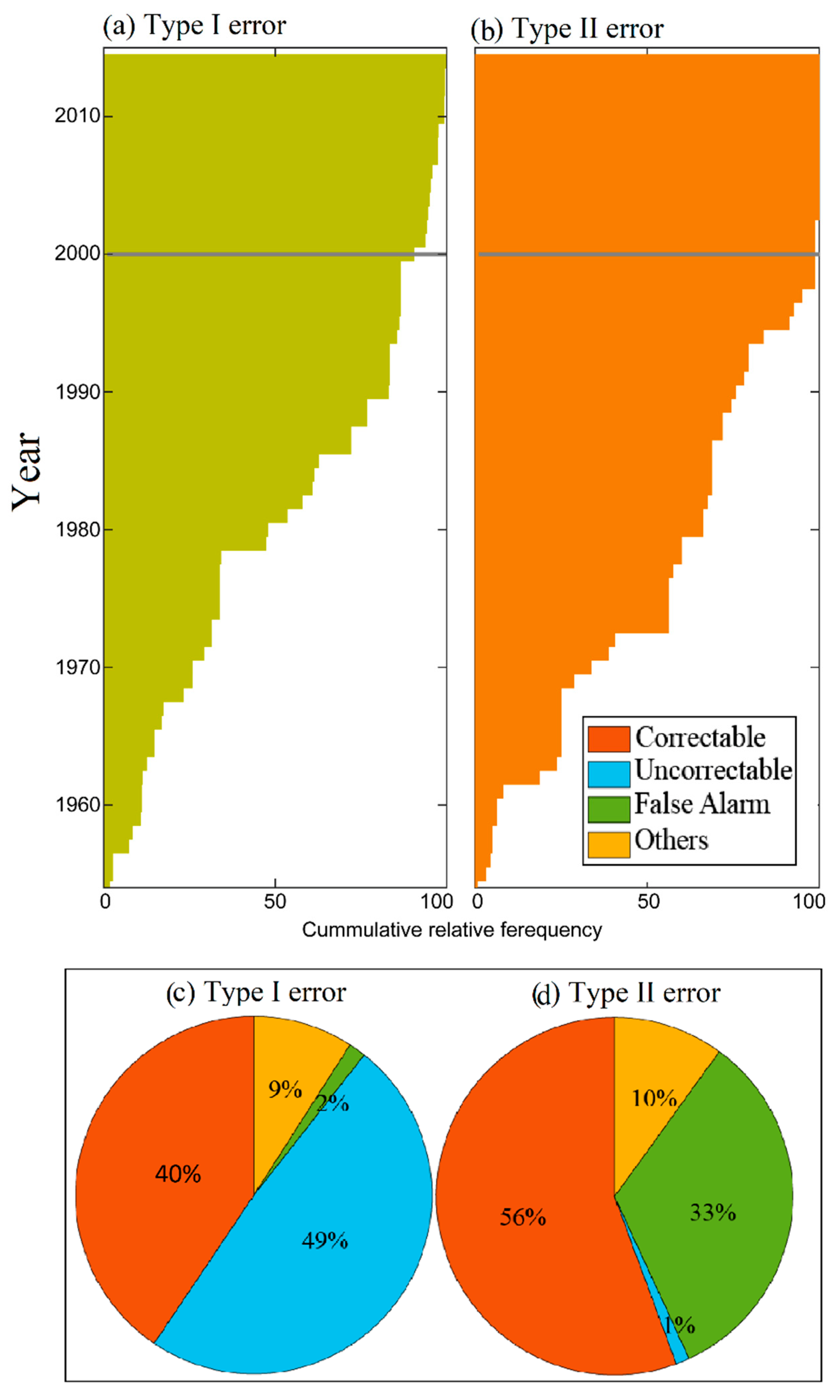
3.1. Rainfall Observation Errors

This section describes the types of rainfall data errors flagged through spatial patterns on the rainfall maps. A False-Negative error shows a gauge with no measured rainfall surrounded by gauges reporting rainfall (Figure 5a). A False-Positive error (Figure 5b) shows a single gauge or an isolated group of gauges with rainfall while no other rainfall is detected on the watershed. Often, the same gauges show a False-Negative error on a previous or subsequent day.
For each of the 6004 days with rainfall in the 62-year period, we visually inspected the map and identified the number of occurrences of each type of error. Figure 6a,b show the temporal changes in error type as cumulative relative frequency (%) for daily rainfall during the period 1954–2014. False-Negative errors are primarily associated with rain gauges not being operational. From the total number of cases, n = 641, 28% occurred during July-September while 72% were observed during October–March. The number of False-Negative errors was largest in the 1980s and mainly during the winter months, which was a period when most of the rain gauges were turned off during the winter due to budgetary restrictions. The percentage of reported False-Negative errors increased from 34% in 1978 to 76% in 1988. False-Positive errors totaled 160 cases during the 62-yr study period and were uniformly distributed through time, except in 1962 and 1970 with 17 and 25 cases, respectively. For both error types, the majority of cases were reported during the analog recording period (pre-2000), indicating that despite the technical expertise of the WGEW technicians and the QAQC procedures in place, human and mechanical equipment errors were sometimes difficult to detect and avoid. Of all the False-Negative errors, 49% of the cases were uncorrectable (unknown causes or lost information, etc.), while 51% were correctable (information available in the original charts or maintenance log) (see Figure 6c,d). For False-Positive errors, the largest contribution to total error was correctable (56%), while the false alarm cases (33%) were not errors but identified as errors due to visual limitations in the inspection of the maps.

3.2. Runoff Observation Errors

This section describes runoff errors flagged by the methods that require a relation between runoff and rainfall: the rainfall-runoff association, lag time, runoff coefficient, and regression methods. The four runoff tests in the three sub-watersheds found a total of 102 questionable events flagged by one or more of the tests for all runoff-producing events: 40 events in WS-04 (12% of events), 28 events in WS-11 (6% of events), and 40 events in WS-06 (6% of events). The tests identified runoff events that were assigned erroneous start times due to malfunctions in the analog clocks or human error. The errors in the runoff start times resulted, in some instances, in runoff occurring before the onset of the rainfall. In other instances, it resulted from excessively large lag times, in excess of the threshold time used. We also identified runoff events with excessively long hydrograph recessions due to sediment blocking the stilling well intakes. This accumulation of sediment slows drainage from the stilling well and consequently affects measurement of the water level. These long recessions are typically replaced with estimated data by fitting a theoretical curve along with a note in the metadata. Unfortunately, some of these types of errors have slipped into the database over the years. These errors were easy to identify with the association method because the 7-h window breaks the long runoff duration data into multiple 7-h runoff events where only the first window will have associated rainfall.
Overall, there were few instances when the four methods in Figure 7 simultaneously flagged runoff events, except when no rainfall is associated with runoff, which tended to be identified by all of the tools. Runoff events recorded before the onset of rain were, for instance, flagged only by the lag time method, especially when the start time between runoff and rainfall was less than 1 h. The lag time method flagged the largest percentage of events (51 to 80% for the three sub-watersheds), followed by the Regression method that identified between 40 and 50% of the flagged events (Figure 7a). The runoff coefficient method flagged the smallest number of events and also showed the largest variability between the watersheds. We did not find a direct relationship between the efficiency of any of the four methods in Figure 7 and the area of the sub-watershed. Each method, regardless of which one is used, was able to identify between 50–75% of the total number of flagged runoff events, but only 7–26% of the errors were detected by all of the methods simultaneously (Figure 7b).
The number of questionable events depends on the threshold values selected for each of the methods. These thresholds require expert knowledge of the watershed being examined, and will vary depending on the characteristics of the watershed. It is also important to note that the threshold values (7-h window in the association method, 1–2 h lag time, etc.) were determined iteratively based on detailed observation of the data. Determining the lag time through consideration of physical processes was beyond the scope of this work. Looking at the computed lag time distribution and plotting the lag time against the total event rainfall depth, though purely subjective, helped us visually define each watershed’s threshold lag time. Errors that were not previously identified in the database were flagged by these tools and confirmed by the metadata (Figure 8). The events in Figure 8 (except b) were flagged using lag time, showing a significant delay of the rainfall that possibly resulted in the runoff. The association method flagged all events in Figure 8 except e and f as all the runoff events did not have associated rainfall within the 4-h window leading to the peak runoff time. The main portion of the hydrograph in Figure 8b (28 July 1966 on watershed WS11) does not seem to have a problem, but the recession that continued over 14 h, with the runoff rate value close to 0.2 cfs (0.006 cumecs), was interpreted as a sequence of runoff events with no associated rainfall.
The runoff coefficient method identified the events in Figure 8a,c,d, and the events in Figure 8e,f were flagged by the regression method (see more in [54]). We applied the plotting tool on the 102 flagged events for which clock issues were the reason for inconsistencies in the data. From visual inspection, 72% of the flagged events were obviously problematic while the rest required more than visual inspection to verify the error. The flagged events had either no rain corresponding to the runoff or the rainfall was recorded after the runoff event started.
About 7% of the flagged events were false alarms, which were flagged mainly by the lag time and association method. False alarms were predominantly from runoff events created by long-duration rainfall events (more than 3 h), which resulted in longer lag times. There were instances in which runoff with multiple peaks or separate runoff events for the same long-duration rain occurred. In some cases, flow was recorded on the flumes only after the contributing area was saturated sufficiently, resulting in a large lag time.

3.3. K2 Simulation Application

When the K2 model is forced by the flagged (erroneous) data, the results are large mismatches between predictions and observations that cannot be explained by any physical processes in the watershed. In Figure 9a, the observed runoff (blue line) is way outside the bounds of the simulated runoff ranges (gray polygon). The simulated runoff ranges represent the model response to the specified rainfall input under a wide range of parameter values. Unless the parameter values are completely inappropriate, the observed hydrograph should fall within the bounds of the simulated hydrographs. This shows that it is impossible to reproduce the rainfall-runoff relation under any physical processes without correcting or removing the errors. This degree of mismatch between simulated and observed data is different from that discussed as a common challenge in modeling hydrologic processes. Lundquist et al., 2014 [9] also described that in these types of errors, efforts at model calibration repeatedly failed under several modeling approaches. The flagged events on 28 July 2010 in Figure 9a showed a runoff delay of 15 h, which is uncharacteristic for the ephemeral responses in Walnut Gulch watersheds. The other three events in Figure 9a illustrate a timing error resulting in runoff before any rainfall was recorded in any of the rain gauges within the watersheds, making any hydrologic analysis and prediction a near-impossible task. Given this, any event-based modeling effort cannot explain the watershed processes, or it will lead to a misinformed understanding of runoff generation processes. In all cases, statistical analysis of the Monte Carlo simulation of the events showed that the best model prediction was the no-runoff simulation. In Figure 9b, the K2 simulation of unflagged data (supposedly error-free data) resulted in observed runoff within the bounds of simulated runoff.

4. Discussion

The future of hydrologic science in light of the accuracies required to understand the impacts of development, management, and other disturbances on landscapes on hydrology and water quality anticipates increased quality data collection, storage, and availability. Errors and mismatches between model outputs and observations are not uncommon in hydrologic science, e.g., [60], which requires creative ways of identifying and correcting the errors that lead to inconsistencies and then to misinterpretations. In the absence of working tools that identify errors using traditional/existing QC measures, hydrologic relationships between the inputs and responses specific to the site are necessary to identify those errors. Before this study, there had not been a systematic study of the link between rainfall and runoff for all of the nested sub-watersheds on WGEW. Though the study here is limited to the formulation of QAQC tools and their application in this exceptional set of hydro-meteorological data that comprises sub-hourly and high spatial resolution observations in a semi-arid environment, the fact that all watershed responses follow similar fundamental hydrologic relations will allow the expansion of the approach to other experimental watersheds and beyond. The strengths and weaknesses of hydrologic logic-based QAQC tools depend on the type of hydrologic regime, the climate, and the dominant processes that affect watershed responses.
The summary of the strengths and weaknesses of each of the methods are given in Table 1. For instance, the daily rainfall maps clearly show if there is a “hole” in the spatial rainfall field due to an inoperable rain gauge. In the lag time method, the high temporal resolution of the data allows identification of errors that would be very difficult using other methods. Such errors include cases when the runoff started 1 min before the beginning of rainfall. It is also important to note that runoff occurring before the start of rainfall, especially by just a few minutes, could be heavy rain on the flume itself. In this case, it is not considered to be runoff, however, any indication of runoff appearing before rainfall is a good reason for suspecting error and flagging the event for further inspection. In this type of data, a plot of rainfall versus runoff (e.g., Figure 3e) may not show the apparent inconsistency. The lag time computation (Equations (1)–(3)) is a simplification that may result in erroneous lag time, especially in long-duration rainfall and for storms moving across the contributing area. The other limitation is the arbitrary definition of threshold lag times, as lag times depend on watershed size, topography, and surface roughness in addition to the spatiotemporal rainfall distribution. The applicability of these methods to other experimental watersheds depends on the type of data, instrumentation density, and temporal resolution of the data. In watersheds that contain a high density of rain gauges and streamflow observations, error detection by way of daily rainfall maps ought to be straightforward. Techniques such as outlier identification, use of interpolated rainfall, etc., were also applied by several researchers [4,8,22,23,26,61]. However, the use of hydrologic signatures for QC applications, which was also described by Yilmaz et al., (2008) [20] and Gupta et al., (1998) [60] in different watersheds, requires an understanding of their unique rainfall-runoff responses as well as observation time steps and the spatial density of the observations. Depending on watershed processes, observation time steps, and the spatial layout of the sensors, some of the QC tools might need adjustment of the procedures presented herein. For instance, in watersheds with groundwater contributions, the association method, lag time, and runoff coefficient method might require base flow separation prior to the application of the methods.
In the WGEW, the ephemeral nature of the headwater watersheds that directly links rainfall forms the basis for much of the data QC. These approaches can be used to improve datasets from similar arid systems such as the USDA-ARS Jornada Experimental Range (Las Cruces, NM, USA), USDA/University Santa Rita Experimental Range (Arizona), Boise State University Dry Creek Experimental Watershed (Idaho, USA), USDA-ARS Reynolds Creek Experimental (Idaho), etc., where event-based runoff and erosion models like RHEM, WEPP, and KINEROS2 are often employed.

5. Conclusions

Prior to this study, there had not been a systematic study of the link between rainfall and runoff for all of the nested sub-watersheds on WGEW. Due to the different forms of errors and how they were introduced into the historical WGEW dataset, multiple QAQC tools were required to reliably flag suspicious events. The respective five tools could be combined into a single, partially automated workflow, but verification through visual inspection by a trained technician or scientist is still necessary. Furthermore, the overlap between the four methods applied in this study was minimal, highlighting the importance of using more than one tool to check for errors. Due to the assumptions in each of our methods, some errors are more likely to be identified by any given method while missing other types of errors. Therefore, it is vital to apply all methods in order to flag as many events as possible, and then confirm the errors using the information available, such as metadata, the original paper-based charts, and the application of graphical visualization tools. Most of the inconsistencies in the WGEW database were due to date and time code errors, events with unreasonably long low-flow periods, false runoff events generated by rainfall on flumes, flume maintenance immediately after a flow, etc. This analysis found that 13% of the days with rainfall and 7% of the runoff events sampled had errors indicating that the prior or existing QAQC protocols are relatively robust. However, considering the widespread use of WGEW data and the substantial investment in data collection, continued investment to improve and develop measurement protocols and QAQC procedures are warranted, e.g., [62].
Given the challenges facing natural resource management, every effort should be made to ensure that accurate long-term datasets are used to understand, plan, and manage sustainable natural resources. Carefully curated datasets will ensure reliable and trustworthy data for monitoring and modeling ecosystem responses. The methods in this study have identified some errors that may otherwise require complex modeling approaches like complete water/energy balance analyses, e.g., [9]. One can transfer these hydrologic relationship-based methods to other similar systems where these principles are applicable or develop new relations by understanding the respective area’s specific fundamental hydrologic relationship.

Author Contributions

Conceptualization, M.B.M., E.M.C.D. and P.H.; methodology, M.B.M., E.M.C.D. and P.H.; software, M.B.M. and E.M.C.D.; validation, M.B.M., E.M.C.D. and A.T.P.; formal analysis, M.B.M.; investigation, M.B.M. and E.M.C.D.; resources, P.H. and D.C.G.; data curation, M.B.M., E.M.C.D. and C.U.; writing, original draft preparation, M.B.M. and E.M.C.D.; writing, review and editing, M.B.M., E.M.C.D., P.H., D.C.G., M.A.K., C.U., G.A. and H.W.; visualization, M.B.M., E.M.C.D. and C.U.; supervision, P.H. and D.C.G. All authors have read and agreed to the published version of the manuscript.

Funding

This research was funded by the Agricultural Research Service, US Department of Agriculture, Washington D.C., USA. The research was a contribution from the Long-Term Agroecosystem Research (LTAR) network. LTAR is supported by the US Department of Agriculture.

Institutional Review Board Statement

Not applicable.

Informed Consent Statement

Not applicable.

Data Availability Statement

Data derived from public domain resources. The data that support the findings of this study are publicly available (https://www.tucson.ars.ag.gov/dap/, accessed on 1 May 2022).

Acknowledgments

We thank the group of dedicated USDA-ARS technicians that for more than 60 years have professionally maintained the network of rain gauges, runoff structures, and general experimental watershed infrastructure used in this study and numerous research projects. Rainfall, runoff, sediment, meteorology and watershed characterization data are freely available from https://www.tucson.ars.ag.gov/dap/, accessed on 1 May 2022. This research was a contribution from the Long-Term Agroecosystem Research (LTAR) network. The US Department of Agriculture is an equal opportunity provider and employer. Mention of a proprietary product does not constitute endorsement by USDA and does not imply its approval to the exclusion of the other products that may also be suitable.

Conflicts of Interest

The authors declare no conflict of interest.

References

  1. Tetzlaff, D.; Carey, S.K.; McNamara, J.P.; Laudon, H.; Soulsby, C. The essential value of long-term experimental data for hydrology and water management. Water Resour. Res. 2017, 53, 2598–2604. [Google Scholar] [CrossRef] [Green Version]
  2. Kleinman, P.J.A.; Spiegal, S.; Rigby, J.R.; Goslee, S.C.; Baker, J.M.; Bestelmeyer, B.T.; Duncan, E.W. Advancing the sustainability of US agriculture through long-term research. J. Environ. Qual. 2018, 47, 1412–1425. [Google Scholar] [CrossRef] [PubMed]
  3. Spiegal, S.; Bestelmeyer, B.T.; Archer, D.W.; Augustine, D.J.; Boughton, E.H.; Boughton, R.K.; Walthall, C.L. Evaluating strategies for sustainable intensification of US agriculture through the Long-Term Agroecosystem Research network. Environ. Res. Lett. 2018, 13, 034031. [Google Scholar] [CrossRef]
  4. Westerberg, I.; Walther, A.; Guerrero, J.L.; Coello, Z.; Halldin, S.; Xu, C.Y.; Lundin, L.C. Precipitation data in a mountainous catchment in Honduras: Quality assessment and spatiotemporal characteristics. Appl. Clim. 2010, 101, 381–396. [Google Scholar] [CrossRef]
  5. Brantley, S.L.; McDowell, W.H.; Dietrich, W.E.; White, T.S.; Kumar, P.; Anderson, S.P.; Gaillardet, J. Designing a network of critical zone observatories to explore the living skin of the terrestrial Earth. Earth Surf. Dyn. 2017, 5, 841–860. [Google Scholar] [CrossRef] [Green Version]
  6. Knapp, A.K.; Smith, M.D.; Hobbie, S.E.; Collins, S.L.; Fahey, T.J.; Hansen, G.J.; Webster, J.R. Past, Present, and Future Roles of Long-Term Experiments in the LTER Network. Bioscience 2012, 62, 377–389. [Google Scholar] [CrossRef] [Green Version]
  7. Collinge, S.K. NEON is your observatory. Front. Ecol. Environ. 2018, 16, 371. [Google Scholar] [CrossRef] [Green Version]
  8. Kauffeldt, A.; Halldin, S.; Rodhe, A.; Xu, C.-Y.; Westerberg, I.K. Disinformative data in large-scale hydrological modelling. Hydrol. Earth Syst. Sci. 2013, 17, 2845–2857. [Google Scholar] [CrossRef] [Green Version]
  9. Lundquist, J.D.; Wayand, N.E.; Massmann, A.; Clark, M.P.; Lott, F.; Cristea, N.C. Diagnosis ofinsidious data disasters. Water Resour. Res. 2015, 51, 3815–3827. [Google Scholar] [CrossRef]
  10. Kautz, M.A.; Holifield Collins, C.D.; Guertin, D.P.; Goodrich, D.C.; van Leeuwen, W.J.; Williams, C.J. Hydrologic model parameterization using dynamic Landsat-based vegetative estimates within a semiarid grassland. J. Hydrol. 2019, 575, 1073–1086. [Google Scholar] [CrossRef]
  11. Korgaonkar, Y.; Guertin, D.P.; Goodrich, D.C.; Unkrich, C.; Kepner, W.G.; Burns, I.S. Modeling urban hydrology and green infrastructure using the AGWA urban tool and the KINEROS2 model. Front. Built Environ. 2018, 4, 1–15. [Google Scholar] [CrossRef] [Green Version]
  12. Goodrich, D.C.; Burns, I.S.; Unkrich, C.L.; Semmens, D.; Guertin, D.P.; Hernandez, M.; Yatheendradas, S.; Kennedy, J.R.; Levick, L. KINEROS2/AGWA: Model Use, Calibration, and Validation. Trans. ASABE 2012, 55, 1561–1574. [Google Scholar] [CrossRef]
  13. Houser, P.R.; Shuttleworth, W.J.; Famiglietti, J.S.; Gupta, H.V.; Syed, K.H.; Goodrich, D.C. Integration of soil moisture remote sensing and hydrologicmodeling using data assimilation. Water Resour. Res. 1998, 34, 3405–3420. [Google Scholar] [CrossRef] [Green Version]
  14. Doll, P.; Siebert, S. Global Modeling of Irrigation Water Requirements. Water Resour. Res. 2002, 38, 8-1–8-10. [Google Scholar] [CrossRef]
  15. Fekete, B.M.; Vörösmarty, C.J.; Roads, J.O.; Willmott, C.J. Uncertainties in precipitation and their impacts on runoff estimates. J. Clim. 2004, 17, 294–304. [Google Scholar] [CrossRef]
  16. Güntner, A. Improvement of Global Hydrological Models Using GRACE Data. Surv. Geophys. 2008, 29, 375–397. [Google Scholar] [CrossRef] [Green Version]
  17. Beven, K.; Westerberg, I. On red herrings and real herrings: Disinformation and information in hydrological inference. Hydrol. Processes 2011, 25, 1676–1680. [Google Scholar] [CrossRef]
  18. Beven, K.J.; Smith, P.J.; Wood, A. On the colour and spin of epistemic error, and what we might do about it. Hydrol. Earth Syst. Sci. 2011, 15, 3123–3133. [Google Scholar] [CrossRef] [Green Version]
  19. Sapač, K.; Rusjan, S.; Šraj, M. Assessment of consistency of low-flow indices of a hydrogeologically non-homogeneous catchment: A case study of the Ljubljanica river catchment, Slovenia. J. Hydrol. 2020, 583, 124621. [Google Scholar] [CrossRef]
  20. Yilmaz, K.K.; Gupta, H.V.; Wagener, T. A process-based diagnostic approach to model evaluation: Application to the NWS distributed hydrologic model. Water Resour. Res. 2008, 44, W09417. [Google Scholar] [CrossRef] [Green Version]
  21. de Vos, L.W.; Leijnse, H.; Overeem, A.; Uijlenhoet, R. Quality control for crowdsourced personal weather stations to enable operational rainfall monitoring. Geophys. Res. Lett. 2019, 46, 8820–8829. [Google Scholar] [CrossRef] [Green Version]
  22. Aguilar, E.; Peterson, T.C.; Obando, P.R.; Frutos, R.; Retana, J.A.; Solera, M.; Mayorga, R. Changes in precipitation and temperature extremes in Central America and northern South America, 1961–2003. J. Geophys. Res. 2005, 110, D23107. [Google Scholar] [CrossRef]
  23. Evett, S.R.; Marek, G.W.; Copeland, K.S.; Colaizzi, P.D. Quality Management for Research Weather Data: USDA-ARS, Bushland, TX. Agrosystems Geosci. Environ. 2018, 1, 1–18. [Google Scholar] [CrossRef] [Green Version]
  24. Kunkel, K.E.; Easterling, D.R.; Hubbard, K.; Redmond, K.; Andsager, K.; Kruk, M.C.; Spinar, M.L. Quality control of pre-1948 cooperative observer network data. J. Atmos. Ocean. Technol. 2005, 22, 1691–1705. [Google Scholar] [CrossRef] [Green Version]
  25. You, J.; Hubbard, K.G.; Nadarajah, S.; Kunkel, K.E. Performance of quality assurance procedures on daily precipitation. J. Atmos. Ocean. Technol. 2007, 24, 821–834. [Google Scholar] [CrossRef]
  26. Eischeid, J.K.; Baker, C.B.; Karl, T.R.; Diaz, H.F. The quality control of long-term climatological data using objetive data analysis. J. Appl. Meteor. 1995, 34, 2787–2795. [Google Scholar] [CrossRef] [Green Version]
  27. Renard, K.G.; Nichols, M.H.; Woolhiser, D.A.; Osborn, H.B. A brief background on the U.S. Department of Agricul-ture Agricultural Research Service Walnut Gulch Experimental Watershed. Water Resour. Res. 2008, 44, W05S02. [Google Scholar] [CrossRef] [Green Version]
  28. Goodrich, D.C.; Heilman, P.; Nearing, M.; Nichols, M.; Scott, R.; Williams, J.; Biederman, J. The USDA-Agricultural Research Service’s Long Term Agroecosystems Walnut Gulch Experimental Watershed. Hydro. Proces. 2021, 35, e14349. [Google Scholar] [CrossRef]
  29. Goodrich, D.C.; Heilman, P.; Anderson, M.; Baffaut, C.; Bonta, J.; Bosch, D.; Bryant, R.; Cosh, M.; Endale, D.; Veith, T.L.; et al. The USDA-ARS Experimental Watershed Network-Evolution, Lessons Learned, Societal Benefits, and Moving Forward. Water Resour. Res. 2021, 57, e2019WR026473. [Google Scholar] [CrossRef]
  30. Baffaut, C.; Baker, J.M.; Biederman, J.A.; Bosch, D.D.; Brooks, E.S.; Buda, A.R.; Demaria, E.M.; Yasarer, L.M. Comparative Analysis of Water Budgets across the U.S. Long-Term Agroecosystem Research Network. J. Hydrol. 2020, 588, 125021. [Google Scholar] [CrossRef]
  31. Fiebrich, C.A.; Crawford, K.C. The impact of unique meteorological phenomena detected by the Oklahoma Mesonet and ARS Micronet on automated quality control. Bull. Am. Meteorol. Soc. 2001, 82, 2173–2187. [Google Scholar] [CrossRef] [Green Version]
  32. Brakensiek, D.L.; Osborn, H.B.; Rawls, W.J. Field Manual for Research in Agricultural Hydrology. U. S.; Department of Agriculture, Agriculture Handbook No. 224; Department of Agriculture, Science and Education Administration: Washington, DC, USA, 1979; 550p. [Google Scholar]
  33. Moran, M.S.; Emmerich, W.E.; Goodrich, D.C.; Heilman, P.; Holifield Collins, C.; Keefer, T.O.; Nearing, M.A.; Nichols, M.H.; Renard, K.G.; Scott, R.L.; et al. Preface to special section on Fifty Years of Research and Data Collection: U.S. Department of Agriculture Walnut Gulch Experimental Watershed. Water Resour. Res. 2008, 44, W05S01. [Google Scholar] [CrossRef] [Green Version]
  34. Nichols, M.H.; Anson, E. Southwest watershed research center data access project. Water Resour. Res. 2008, 44, W05S03. [Google Scholar] [CrossRef] [Green Version]
  35. Renard, K.G.; Lane, L.J.; Simanton, J.R.; Emmerich, W.E.; Stone, J.J.; Weltz, M.A.; Goodrich, D.C.; Yakowitz, D.S. Agricultural impacts in an arid environment: Walnut Gulch studies. Hydrol. Sci. Technol. 1993, 9, 149–159. [Google Scholar]
  36. Demaria, E.M.C.; Goodrich, D.C.; Kunkel, K.E. Evaluating the reliability of the U.S. Cooperative Observer Program precipitation observations for extreme events analysis using the LTAR network. J. Atmos. Ocean Technol. 2019, 36, 317–332. [Google Scholar] [CrossRef] [Green Version]
  37. Roeske, R.H.; Garrett, J.M.; Eychaner, J.H. Floods of October 1983 in southeastern Arizona, U.S. Geol. Surv. Water Resour. Investig. Rep. 1989, 98-4225-c. [Google Scholar]
  38. Keefer, T.O.; Renard, K.G.; Goodrich, D.C.; Heilman, P.; Unkrich, C.L. Quantifying Extreme Precipitation Events and their Hydrologic Response in Southeastern Arizona. J. Hydrol. Eng. 2015, 21, 1–10. [Google Scholar] [CrossRef] [Green Version]
  39. Goodrich, D.C.; Lane, L.J.; Shillito, R.M.; Miller, S.N.; Syed, K.H.; Woolhiser, D.A. Linearity of basin response as a function of scale in a semiarid watershed. Water Resour. Res. 1997, 33, 2951–2965. [Google Scholar] [CrossRef]
  40. Keefer, T.O.; Moran, M.S.; Paige, G.B. Long-term precipitation database, Walnut Gulch Experimental Watershed, Arizona, United States. Water Resour. Res. 2008, 44, W05S07. [Google Scholar] [CrossRef] [Green Version]
  41. Garcia, M.; Peters-Lidard, C.D.; Goodrich, D.C. Spatial interpolation of precipitation in a dense gauge network for monsoon storm events in the southwestern United States. Water Resour. Res. 2008, 44, W05S13. [Google Scholar] [CrossRef] [Green Version]
  42. Smith, R.E.; Chery, D.L.; Renard, K.G.; Gwinn, W.R. Supercritical Flow Flumes for Measuring Sediment-Laden Flow; USDA ARS Technical Bulletins 1655; US Department of Agriculture, Agricultural Research Service: Washington, DC, USA, 1982.
  43. Stone, J.J.; Nichols, M.H.; Goodrich, D.C.; Buono, J. Longterm runoff database, Walnut Gulch Experimental Watershed, Arizona, United States. Water Resour. Res. 2008, 44, W05S05. [Google Scholar] [CrossRef] [Green Version]
  44. Nichols, M.H.; Stone, J.J.; Nearing, M.A. Sediment database, Walnut Gulch Experimental Watershed, Arizona, United States. Water Resour. Res. 2008, 44, W05S06. [Google Scholar] [CrossRef] [Green Version]
  45. Keefer, T.O.; Unkrich, C.L.; Smith, J.R.; Goodrich, D.C.; Moran, M.S.; Simanton, J.R. An event-based comparison of two types of automated-recording, weighing bucket rain gauges. Water Resour. Res. 2008, 44, W05S12. [Google Scholar] [CrossRef] [Green Version]
  46. Osborn, H.B.; Lane, L.J.; Myers, V.A. Rainfall/watershed relationships for southwestern thunderstorms. Trans. ASAE 1980, 23, 82–87. [Google Scholar] [CrossRef]
  47. Reich, B.M.; Osborn, H.B. Improving Point Rainfall Prediction with Experimental Data? Mississippi State University: Starkville, MS, USA, 1982; pp. 41–54. [Google Scholar]
  48. Osborn, H.B.; Lane, L. Precipitation-runoff relations for very small semiarid rangeland watersheds. Water Resour. Res. 1969, 5, 419–425. [Google Scholar] [CrossRef]
  49. Simanton, J.R.; Osborn, H.B. Runoff estimates for thunderstorm rainfall on small rangeland watersheds. In Hydrology and Water Resources in Arizona and the Southwest; Arizona-Nevada Academy of Science: Flagstaff, AZ, USA, 1983; Volume 13, pp. 9–15. [Google Scholar]
  50. Kampf, S.K.; Faulconer, J.; Shaw, J.R.; Lefsky, M.; Wagenbrenner, J.W.; Cooper, D.J. Rainfall thresholds for flow generation in desert ephemeral streams. Water Resour. Res. 2018, 54, 9935–9950. [Google Scholar] [CrossRef]
  51. Syed, K.H.; Goodrich, D.C.; Myers, D.E.; Sorooshian, S. Spatial characteristics of thunderstorm rainfall fields and their relation to runoff. J. Hydrol. 2003, 271, 1–21. [Google Scholar] [CrossRef] [Green Version]
  52. Goodrich, D.C.; Chehbouni, A.; Goff, B.; MacNish, B.; Maddock, T.; Moran, S.U.S.A.N.; Yucel, I. Preface paper to the Semi-Arid LandSurface-Atmosphere (SALSA) program special issue. Agric. For. Meteorol. 2000, 105, 3–20. [Google Scholar] [CrossRef]
  53. Yatheendradas, S.; Wagener, T.; Gupta, H.; Unkrich, C.; Goodrich, D.; Schaffner, M.; Stewart, A. Understanding uncertainty in distributed flash flood forecasting for semiarid regions. Water Resour. Res. 2008, 44, W05S19. [Google Scholar] [CrossRef]
  54. Bitew, M.M.; Goodrich, D.C.; Demaria, E.; Heilman, P.; Nichols, M.; Levick, L.; Unkrich, C.L.; Kautz, M. Multi-parameter regression modeling for improving the quality of measured rainfall and runoff data in densely instrumented watersheds. J. Hydrol. Eng. 2019, 24, 04019036. [Google Scholar] [CrossRef] [Green Version]
  55. Houser, P.; Goodrich, D.; Syed, K. Runoff, precipitation, and soil moisture at Walnut Gulch. In Spatial Patterns in Catchment Hydrology: Observations and Modelling; Grayson, R., Blöschl, G., Eds.; Cambridge University Press: Cambridge, UK, 2000; pp. 125–157. [Google Scholar]
  56. Akaike, H. Information Theory and An Extension of the Maximum Likelihood Principle. In International Syrup on Information Theory, 2nd ed.; Petrov, B.N., Csaki, F., Eds.; Akademia Kiado: Budapest, Hungary, 1973; pp. 267–281. [Google Scholar]
  57. SCS (Soil Conservation Service). Hydrology National Engineering Handbook; SCS: Washington, DC, USA, 1972. [Google Scholar]
  58. Semmens, D.; Goodrich, D.C.; Unkrich, C.L.; Smith, R.E.; Woolhiser, D.A.; Miller, S.N. Hydrological Modelling in Arid and Semi-arid Areas; KINEROS2 and the AGWA Modeling Framework; Cambridge University Press: Cambridge, UK, 2005; pp. 49–68. [Google Scholar]
  59. Smith, R.E.; Goodrich, D.C.; Woolhiser, D.A.; Unkrich, C.L. KINEROS2—A KINematic Runoff and EROSion Model. In Computer Models of Watershed Hydrology; Singh, V.P., Ed.; Water Resources Publication: Highlands Ranch, CO, USA, 1995; pp. 697–732. [Google Scholar]
  60. Gupta, H.V.; Wagener, T.; Liu, Y. Reconciling theory with observations: Elements of a diagnostic approach to model evaluation. Hydrol. Processes 2008, 22, 3802–3813. [Google Scholar] [CrossRef]
  61. McMillan, H.; Krueger, T.; Freer, J. Benchmarking observational uncertainties for hydrology: Rainfall, river discharge and water quality. Hydrol. Processes 2012, 26, 4078–4111. [Google Scholar] [CrossRef]
  62. McCord, S.E.; Webb, N.P.; Van Zee, J.W.; Burnett, S.H.; Christensen, E.M.; Ericha, C.M.; Laney, C.M.; Lunch, C.; Maxwell, C.; Karl, J.W.; et al. Provoking a cultural shift in data quality. Front. Ecol. Environ. 2021, 71, 647–657. [Google Scholar] [CrossRef]
Figure 1. Illustration showing (a) the Walnut Gulch Experimental Watershed (WGEW) geographic location with associated sub-basins (primary (WS-04, WS-06, and W-011) delineated in bold lines and secondary delineated in thin lines), average total summer rainfall (2000–2017), and spatial distribution of 99 rain gages; (b) a US Department of Agriculture digital weighing rain gage typical to WGEW; and (c) typical flume in WGEW, example from WS-06-Flume 6.
Water 14 02198 g001
Figure 2. The flow chart of visual inspection of the daily interpolated rainfall maps to identify the inconsistencies in the recordings. The identified inconsistencies were cross-checked using previous and flowing day interpolated maps. False-Negative recording errors are errors due to turned off rain gauges or missing gauges whose records are referred to in the metadata, while False-Positive recording errors are errors resulting from date coding.
Water 14 02198 g002
Figure 3. Schematic description of the five approaches used for runoff quality assurance and quality control (QAQC). (a) Rainfall-runoff association method, (b) Lag time, (c) Runoff coefficient, (d) Regression method, and (e) plots of runoff and corresponding rainfall. The red “x” represents the estimated runoff rate when hydrograph recordings are truncated from the long tail baseflow due to the stilling basin’s siltation.
Water 14 02198 g003
Figure 4. Example showing questionable events identified by lag time method and visual aid to determine the value of threshold lag time for WS-11. The suspicious events are those with outlier lag times. The threshold lag time for WS-11 based on the distribution of the computed lag time values is 70 min, where it showed clear separation from the rest of the calculated values.
Water 14 02198 g004
Figure 5. Rainfall errors identified with the aid of rainfall maps, (a) False-Negative recording error that shows zero rainfall is a large portion of the watershed while in reality those gauges were turned off and (b) False-Positive recording errors: a closer look at inconsistent and abrupt changes in interpolation field showed errors resulting from date coding.
Water 14 02198 g005
Figure 6. Cumulative relative frequency of days with errors in the rainfall dataset from 1954 to 2014 (a,b) and the percentage contribution of each source of error to total error (c,d). The horizontal line in a and b indicates the date when the analog system was replaced by the digital system.
Water 14 02198 g006
Figure 7. (a) Percentage of events flagged by the four of the five methods for the three sub-watersheds, (b) Percentage of the total number of flagged events identified by one to four methods simultaneously.
Water 14 02198 g007
Figure 8. Examples of flagged runoff events, showing runoff (black line) and rainfall from multiple gauges (gray lines) on the inverted y-axis. The solid blue line represents conditional mean of the different rain gauges in the watersheds. The figure shows excessively delayed runoff in (a,c), runoff events not associated with the corresponding rainfall in (b,d), and runoff occurred before the rainfall was being recorded in (e,f).
Water 14 02198 g008
Figure 9. Event scale K2 modeling of runoff processes using flagged and unflagged events. The simulated runoff ranges (gray polygon) representing possible processes in Walnut Gulch and observed runoff (blue line). (a) Example of mismatch in flagged events simulation, and (b) Examples of unflagged events simulation representing error-free data.
Water 14 02198 g009
Table 1. Pros and cons of the four methods implemented for the runoff QC.
MethodProsCons
Rainfall Interpolation method (Rainfall)Effectively identified rain gauge errors through the visual inspection of rainfall fields at daily time scale.Inaccurate times coded to rainfall within a given day are hard to detect.
Implementation at sub-daily time step is time consuming.
It does not include identification of runoff.
Lag time method (Runoff)Identified erroneous runoff events with runoff start time as early as one minute before the rainfall start time.
Excessively large lag times indicate clear errors in the timing of either the runoff or the rainfall.
Runoff events triggered by heavy rain on the flumes could be erroneously flagged.
Long duration rainfall and storms moving across the contributing areas may result in erroneous lag time.
A threshold lag time value depends on the size of the watershed.
The center of mass of the excess rainfall was computed for one of the rain gauges in the watershed, which may not be representative of the watershed scale observed rainfall.
Association method (Runoff)Effectively identified runoff events without associated rainfall.
The 7-h window, i.e., 3 h preceding and 3 h succeeding the maximum observation, was found to be a reasonable window for the rainfall or runoff.
Effectively identified erroneous events with excessively long low flows once the runoff had receded.
An hourly mean of multiple rain gauges in the watershed was used which may remove some important information from the rainfall observations.
An arbitrary threshold rainfall depth of less than 1 mm was considered as no rain. In some cases, the threshold value was a false alarm.
It is hard to detect errors with short time error code shifts (<1 h).
Runoff Coefficient (Runoff)Easy to implement in multiple sub-watersheds.
Effectively identified runoff events without associated rainfall.
Sensitive to the threshold time used for computing C.
Regression method (Runoff and rainfall)Successfully applied to all events regardless of observed runoff data.Predicted runoff largely underestimated observations.
High likelihood of predicting runoff from a given rainfall event for which no observations were available.
Publisher’s Note: MDPI stays neutral with regard to jurisdictional claims in published maps and institutional affiliations.

