Modeling the 2D Inundation Simulation Based on the ANN-Derived Model with Real-Time Measurements at Roadside IoT Sensors

Abstract

This study aims to develop a smart model for the two-dimensional (2D) inundation simulation based on the derived artificial neural network (ANN) model with real-time measurements at the roadside IoT (Internet of Things) sensors; in detail, the flooding zones and associated area can be quantified by combining the inundation-depth estimates at the ungauged locations (defined by the virtual IoT sensor, VIOT) via the corresponding inundation-estimation equations, established using the ANN-derived model with the measurements at the IoT sensors (named SM_EID_VIOT model). Moreover, the resulting inundation-depth estimates at the ungauged locations from the proposed SM_EID_VIOT model can be improved by means of the real-time error-correction approach for the 2D inundation simulation. To demonstrate the reliability of the results from the proposed SM_EID_VIOT model, 1000 simulations of the rainfall-induced flood events within the study area of the Miaoli City of Northern Taiwan are generated as the model-training and validation datasets. Consequently, the proposed SM_EID_VIOT could estimate the inundation depths with an acceptable accuracy at the ungauged locations in time and space based on a low root mean square error (RMSE) of under 0.01 m and a high coefficient of determination (R²) of over 0.8; and it also can delineate the flooding zone to quantify the corresponding area in high reliability in terms of the precision ratio of about 0.7.

1. Introduction

Due to climate change and extreme rainstorm events, rainfall-induced flood frequently occurs, causing severe damage to people’s lives and property [1]. Therefore, modeling flood simulation plays a vital role in providing relevant information on preventing flood-induced hazards. When carrying out the flood early warning to mitigate the flood-induced hazard, the flooding information is necessarily measured and estimated in advance to delineate the potential inundation regions and estimate the inundation depths at the gauged and ungauged locations. Recently, because of the establishment of the levee system, flood is rarely triggered by overtopping from the embankments; on the contrary, inundation frequently occurs in urban areas attributed to the failure of the surface drainage system [2]; thus, regarding the flood information issued, the inundation depths at the specific locations and induced flooding area are needed for detecting the detail of flood-induced hazard/disaster to configure the facing supplement.

The hydraulic/hydrodynamic models are comprehensively utilized to numerically exhibit the complicated hydrological process and flood dynamics [3] under consideration of the precipitation observations/forecasts. That is, through the hydraulic numerical models, the inundation depths and the potential flooding zones, as well as the associated area, can be estimated in the case of the various types of rainfalls, such as the design rainfall events of the different return periods and the precipitation forecasts as well as observations [2,4,5,6,7]. Despite the hydraulic numerical models being applied in the flood simulation, their reliability and accuracy might be affected by the uncertainties in the requirement of sufficient observations, the complex model structures, hydrological/hydraulic features, and extensive computation time [3,4,8]. Recently, the artificial intelligence (AI) models have been comprehensively employed in flood-induced inundation based on machine learning (ML) techniques [9]. Of the relevant ML approaches commonly used, the two types of natural network (NN) methods, the convolutional NN (CNN) and artificial NN (ANN) models, are both more efficiently established for describing the nonlinear mathematic relationships by configuring the linear multi-layer network with all possible predictor variables under the multiple training algorithm. In addition to the input and output layers, the CNN model includes the convolution and pooling layers, differing from the ANN model with the hidden layers.

With computation power increasing, the CNN-based and ANN-derived models are widely applied to the relevant hydrological/hydraulic analysis, especially in flood-related simulations/forecasts [1,3,4,9,10,11,12,13,14]. In detail, the CNN-based model is derived via the neutral network, comprising the convolution, pooling, and fully connected layers, requiring extensive 2D data (i.e., gridded data) as datasets (e.g., the image and videos) for the model training and application [3,4,15]; accordingly, the CNN model can efficiently provide the single model output from the grid-format model inputs. That is to say, the CNN-based model is advantageous concerning the 2D flood simulations for predicting or estimating the spatiotemporal flood-related variates (e.g., the inundation depths and corresponding area) [9]. The CNN-derived models have been proven to be efficiently implemented in the 2D flood forecast with the gridded inputs (such as the grid-based radar precipitation); however, without the mixed data, including the single dataset (e.g., at-site water level) and grid-format data under high-performance computing servers [3], it might cause the extensive computation time in the model training and application. Additionally, the resulting inundation results from the CNN-based models are just identified from the existing flood-related images database solved in the pooling layers used in the model training without considering the changes in the required hydrological factors (e.g., the precipitation) and merely reflecting the experimental flooding conditions in terms of the real-time recorded observations at the gauges and IoT (internet of thing) sensors.

In contrast, the ANN model with the multilayer artificial neural networks is a pioneering approach for the AI models [15] in which the activation function, number of hidden layers, and associated neurons should be known in advance; moreover, the corresponding weights of neurons at various layers are commonly calibrated via the backpropagation (BP) algorithm. However, the ANN model is hardly configured due to the problems with the neural network, e.g., the difficulty of determining the proper network structures, unexplained behavior of the network, the difficulty of evaluating the mathematical shape of a nonlinear relationship between outputs and inputs, and extensive computation time of model training [16,17]. Nevertheless, the ANN-derived model can establish the linear and nonlinear relationships between various input-output combinations by configuring the linear multi-layer network using all possible predictor variables through the multiple training algorithm, especially for hydrological forecasts, such as the precipitation, discharge, and water level [16].

However, the simulations of spatiotemporal hydrological variables are barely carried out by the ANN-derived models with simultaneous considering the correlation in time and space [18]. Nonetheless, the ANN-derived model is advantageous for estimating the at-site hydrological variables; thus, the spatiotemporal hydrological variable could be obtained by aggregating the temporal results from the ANN-derived models at various locations or forecasting the temporal average via the ANN-derived models [19,20]. As a result, in this study, the 2D inundation simulation intends to be accomplished by combining the gridded inundation depths estimated by the ANN-derived model for different locations. Moreover, it is well known that the roadside IoT sensors have recently been implemented in the real-time measurement of the hydrological variables (e.g., water levels), and they are proven to be advantageous to water conservation computerization [1,9,21]. Therefore, to efficiently estimate the inundation depths at all ungauged locations (named virtual IoT sensors, VIOTs) with the real-time measurements at the roadside IoT sensors for delineating the flooding zones, this study aims to model the 2D inundation simulation based on the ANN-derived model; in detail, the relationship of the estimated inundation depths at each ungauged location with the real-time measurements at the roadside IoT sensors (VIOTs) could be established based on the ANN-derived model (called the SM_EID_VIOT model).

Additionally, to boost the reliability of the proposed SM_EID_VIOT model in the 2D inundation simulation, a significant number of rainfall-induced inundation simulations are treated as the training dataset. Additionally, in seeking to enhance the accuracy of the resulting inundation-depth estimates at the ungauged locations, the proposed SM_EID_VIOT model is developed by coupling it with the real-time error-correction technique regarding the hydrological variables based on the different estimations and observations at the previous times during the rainfall-induced flood event. It is expected that the proposed SM_EID_VIOT can provide the inundation depths at the ungauged locations with high reliability and delineate the flooding area induced, which is helpful for the early warning operation.

2. Methodology

2.1. Model Concept

As mentioned in Section 1, an ANN-derived inundation-depth estimation model at the ungauged locations (named the virtual IoT sensors, VIOT) is developed herein, called the SM_EID_VIOT model. In seeking to facilitate the accuracy and reliability of the results from the proposed SM_EID_VIOT model, a significant number of the regional rainstorms are simulated via the stochastic modeling for generating the gridded short-term rainstorms (i.e., SM_GSTR model) [22]; they are then adopted in reproducing numerous two-dimension (2D) inundation simulations employing the hydraulic dynamic numerical model (i.e., SOBEK) [23]. Thus, the resulting datasets, containing the simulations of the gridded rainstorms and the corresponding inundation depths at all grids, including the ungauged locations and the roadside IoT sensors, could be utilized in the development of the proposed SM_EID_VIOT model by training the ANN_derived model ANN_GA-SA_MTF model [1] for quantifying the relationships of the inundation depths between the inundation depths at the ungauged locations and the IoT sensors. Afterward, as a result of reducing the uncertainties in the observations and model parameters which commonly influences the reliability and accuracy of the model outputs, the proposed SM_EID_VIOT model is coupled with the real-time error correction method for 2D inundation simulation, RTEC_2DIS [2] to immediately adjust the resulting inundation-depth estimates at the ungauged locations from the proposed SM_EID_VIOT model. Eventually, by overlaying the resulting inundation-depth estimates at all grids on the digital elevation map (DEM), the flooding zone can be delineated, and the corresponding inundation area can be accordingly quantified by multiplying the number of the inundated grids multiplied by the size of the grid (i.e., the spatial resolution in the DEM).

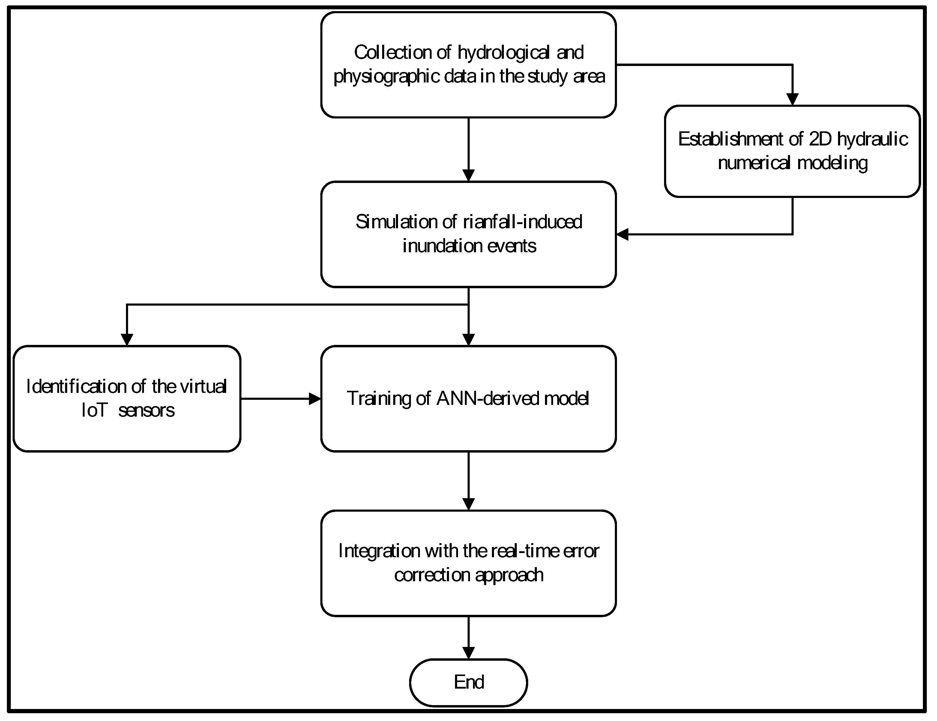
To obtain more reliable and accurate results from the proposed SM_EID_VIOT model, regarding the model development, 1000 simulations of the rainfall-induced flood events are produced in advance, and the real-time error correction method of the resulting gridded inundation depths from the proposed SM_EID_VIOT model is carried out in the model application. As a result, the framework of the model development and application can comprise five parts: (1) generation of the gridded rainstorm events in the study area; (2) 2-D inundation simulations using the well-known hydrodynamic numerical modeling and (3) identification of the ungauged locations as the virtual IoT sensors; (4) establishment of an ANN-derived model for estimating inundation depths at the ungauged locations and (5) integration with the real-time error method as shown in Figure 1. The aforementioned relevant methods and concepts are addressed below:

2.2. Simulation of Rainfall-Induced Inundation Events

Generally speaking, an excellent training dataset is essential in training the ANN-based models. Thus, in this study, to train the ANN_GA-SA_MTF model of interest, a significant number of the rain fields consisting of the rainstorms at all grids in the study reproduced by the SM_GSTR model are used in the 2D inundation simulation carried out by the SOBEK model to obtain the gridded inundation-depth simulations in the study area.

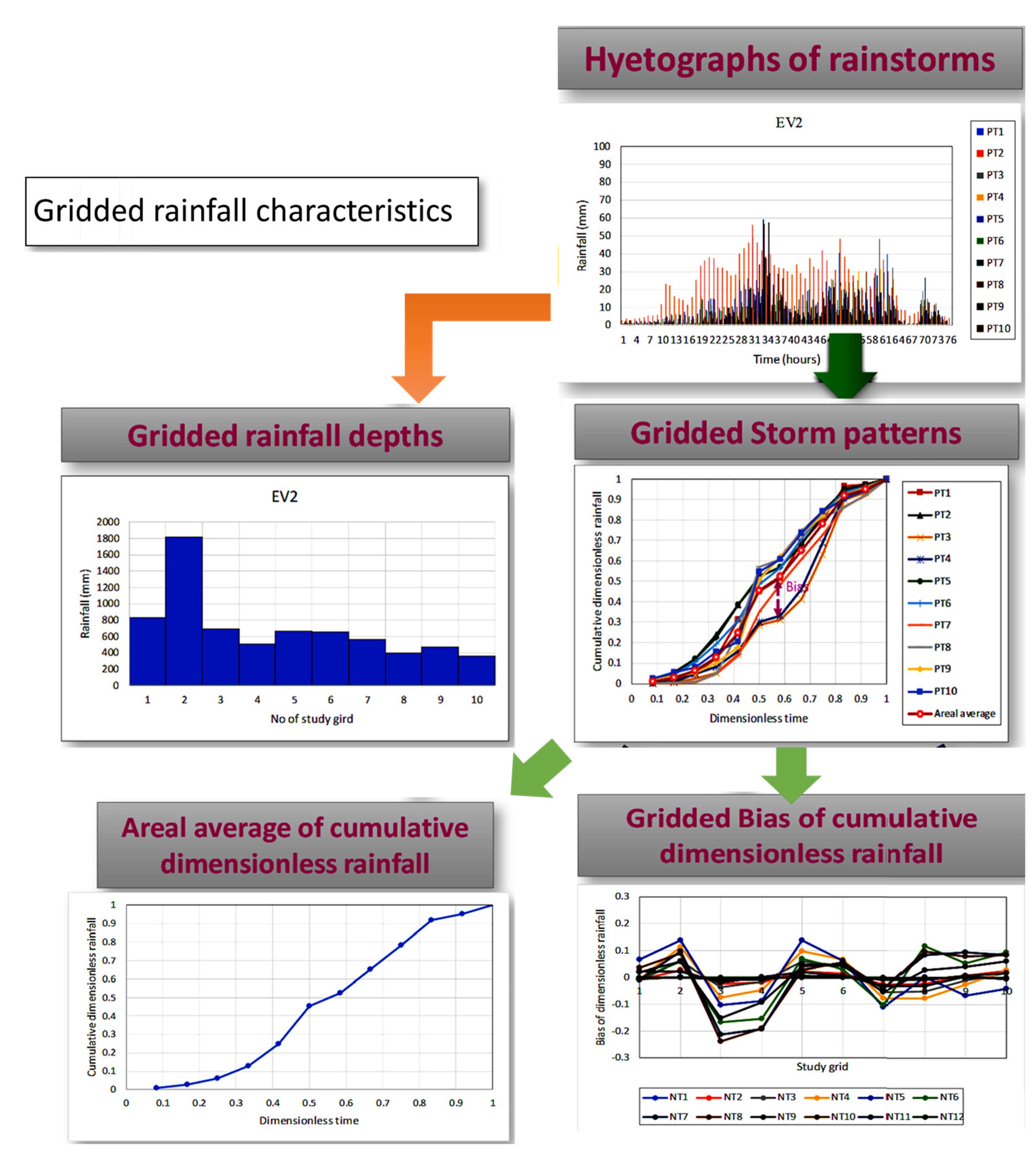
Regarding the SM_GSTR model, the event-based rainstorm is characterized in terms of three rainfall characteristics, the event-based rainfall duration, gridded rainfall depths (regarded as the spatial variates), and gridded storm depths comprised of the dimensionless rainfalls at the various dimensionless times (treated as the Spatio-temporal correlated variates); as for the gridded storm pattern, it can be grouped into two components, the areal average of the dimensionless rainfalls (i.e., the storm pattern) and the associated deviations at the various dimensionless times. Figure 2 graphically illustrates the process of characterizing the gridded rainstorms into the five gridded rainfall characteristics.

After that, the statistical analysis for the gridded rainfall characteristics is performed to quantify their uncertainties in time and space, including the first four statistical moments, correlation coefficients, and the appropriate probability functions. However, a great number of the gridded rainfall characteristics are re-produced using the correlated multivariate Monte Carlo simulation method [24] with the normalized-based algorithms, including the standardized, orthogonal, and inverse transformations, in which their correlations are calculated via the Nataf distribution [25]:

$${\mathsf{\rho }}_{ij}=\underset{-\infty }{\overset{\infty }{{\displaystyle \int }}}\underset{-\infty }{\overset{\infty }{{\displaystyle \int }}}\lfloor \frac{x_i-{\mu }_i}{{\sigma }_i}\rfloor \lfloor \frac{x_j-{\mu }_j}{{\sigma }_j}\rfloor {\varnothing }_{ij}(⟨z_i,z_j|{\rho }_{ij}^{*}⟩){\mathrm{dz}}_i{\mathrm{dz}}_j$$

(1)

$$z_i=\frac{x_i-{\mu }_i}{{\sigma }_i};z_j=\frac{x_j-{\mu }_j}{{\sigma }_j}$$

(2)

where $x_i$ and $x_j$ are the correlated variables at the points i and j, respectively, with the means ${\mu }_i$ and ${\mu }_j$, the standard deviations ${\sigma }_i$ and ${\sigma }_j$, and the correlation coefficient ${\rho }_{ij}$; $z_i$ and $z_j$ are corresponding bivariate standard normal variables to the variable $x_i$ and $x_j$ with the correlation coefficient and the joint standard normal density function ${\varnothing }_{ij}\left(·\right)$. Eventually, the simulations of the gridded storm patterns are reproduced by combing the simulations of the areal averages of dimensionless cumulative rainfalls and the associated gridded bias; then, the gridded rainstorms are emulated by coupling the simulated storm patterns at all grids with the simulations of the gridded rainfall depths for the simulated event-based duration. The detailed introduction to the SM_GSTR model can be referred to in the investigation by Wu et al. [22].

Afterward, using the SOBEK model comprehensively applied in the 2D inundation simulation, especially in regions with various hydraulic structures, a significant number of simulations of the rainfall-induced flood events could be accordingly accomplished with a large number of simulated gridded rainstorms. The resulting massive rainfall-induced inundation simulations would be treated as the training and validating datasets for the proposed SM_EID_VIOT model.

2.3. Identification of the Virtual IoT (VIOT) Grids

Based on the results derived from the simulation of the gridded rainstorm events within the study area, a 2D inundation simulation with high spatial and temporal resolution could be used to determine the locations of the virtual IoT (VIOT) grids. In this study, the VIOT grids are defined as the locations in association with high flooding risk quantified from the above rainfall-induced inundation simulations by the following equation:

$$\begin{gathered} P_f\left(h_f>0\right)=\frac{{{\displaystyle \sum }}_{i=1}^{N_{GRS}}\left(I_f\left(h_f^i\right)\right)}{N_{GRS}} \\ {I}_f\left(h_f^i\right)=1,ifmax\left(h_f\right)>0_{}^{} \\ {I}_f\left(h_f^i\right)=0,ifmax\left(h_f\right)=0_{}^{} \end{gathered}$$

(3)

where $I_f\left(h_f^i\right)$ is the flooding indicator, and $max\left(h_f\right)$ stands for the maximum value of gridded inundation depth $max\left(h_f\right)$ resulting from a rainfall-induced flood event. In Equation (7), if the maximum of gridded inundation depth is greater than zero, the corresponding flooding probability $I_f\left(h_f^i\right)$ is equal to one; otherwise, it is similar to 0.

Consequently, the locations of the VIOT grids can be recognized based on the results from the quantification of gridded flooding risk within the region considered; namely, in this study, the VIOT is defined as the grid in association with the nonzero flooding probability.

2.4. Artificial Neural Network Model Associated with Multiple Transfer Functions

In this study, to reduce the variation in the outputs of the ANN-derived models attributed to the uncertainties in the selection of the activation/transform functions, the calibration of the weights between layers, the ANN_GA-SA_MTF model [1] is used to establish the relationship between the inundation-depth estimates at virtual spots and observations at the practical IoT sensors. The ANN_GA-SA_MTF model is developed by adopting the network structure of three layers with the multiple transfer functions (see

Table 1. The formula for estimating the number of hidden neurons [1].

No of Formula	Formula
1	$N_{HN}=\left(\sqrt{1+8\times N_{IP}}-1\right)/2$
2	$N_{HN}=N_{IP}-1$
3	$N_{HN}=\raisebox{1ex}{$2\times N_{IP}$}\!\left/ \!\raisebox{-1ex}{$N_{IP}$}\right.$+1
4	$N_{HN}=\sqrt{N_{IP}\times N_{OP}}$
5	$N_{HN}=2^{N_{IP}}-1$
6	$N_{HN}=\raisebox{1ex}{$\left[4\times {(N_{IP})}^2+3\right]$}\!\left/ \!\raisebox{-1ex}{$\left[{(N_{IP})}^2-8\right]$}\right.$

) and the number of the associated neurons calculated using the equations (see

Table 2. Transform functions commonly used [1].

Transfer Function		Formula	Derivative
TF1	Logistic(soft step, Sigmoid)	$\mathrm{f}\left(\mathrm{x}\right)=\frac{1}{1+e^{-\propto x}}$	$\mathrm{f}\prime \left(\mathrm{x}\right)=\mathrm{f}\left(\mathrm{x}\right)\left(1-\mathrm{f}\left(\mathrm{x}\right)\right)$
TF2	Tanh	$\mathrm{f}\left(\mathrm{x}\right)=\tanh \left(\mathrm{x}\right)=\frac{2}{1+e^{-2\propto x}}-1$	$\mathrm{f}\prime \left(\mathrm{x}\right)=1-f{\left(x\right)}^2$
TF3	Arctan	$\mathrm{f}\left(\mathrm{x}\right)=ta{n}^{-1}\left(\propto x\right)$	$\mathrm{f}\prime \left(\mathrm{x}\right)=\frac{1}{{\left(\propto x\right)}^2+1}$
TF4	Identity	$\mathrm{f}\left(\mathrm{x}\right)=\propto$ x	$\mathrm{f}\prime \left(\mathrm{x}\right)= \propto$
TF5	Rectified linear unit (ReLU)	$\mathrm{f}\left(\mathrm{x}\right)=\{\begin{array}{c}0 for x<0\\ x for x\ge 0\end{array}$	$\mathrm{f}\prime \left(\mathrm{x}\right)=\{\begin{array}{c}0 for x<0\\ 1 for x\ge 0\end{array}$
TF6	Parameteric rectified linear unit (PReLU, leaky ReLU)	$\mathrm{f}\left(\mathrm{x}\right)=\{\begin{array}{c}\propto x for x<0\\ x for x\ge 0\end{array}$	$\mathrm{f}\prime \left(\mathrm{x}\right)=\{\begin{array}{c}\propto for x<0\\ 1 for x\ge 0\end{array}$
TF7	Exponential linear unit(ELU)	$\mathrm{f}\left(\mathrm{x}\right)=\{\begin{array}{c}\propto \left(e^x-1\right)for x<0\\ x for x\ge 0\end{array}$	$\mathrm{f}\prime \left(\mathrm{x}\right)=\{\begin{array}{c}f\left(x\right)+\propto for x<0\\ 1 for x\ge 0\end{array}$
TF8	Inverse abs (IA)	$\mathrm{y}\left(\mathrm{x}\right)\frac{x}{1+\left|\propto x\right|}$	$\mathrm{y}\prime \left(\mathrm{a}\right)=\frac{1}{{\left(1+\left|a\propto x\right|\right)}^2}$
TF9	Rootsig (RS)	$\mathrm{y}\left(\mathrm{x}\right)=\frac{\propto x}{1+\sqrt{1+{\left(\propto x\right)}^2}}$	$\mathrm{y}\prime \left(\mathrm{x}\right)=\frac{1}{\left(1+\sqrt{1+{\left(\propto x\right)}^2}\right)\sqrt{1+a{\left(\propto x\right)}^2}}$
TF10	Sech function (SF)	$\mathrm{y}\left(\mathrm{x}\right)=\frac{2}{\exp \left(\propto x\right)+\exp \left(-\propto x\right)}$	$\mathrm{y}\prime \left(\mathrm{x}\right)=-\mathrm{y}\left(\mathrm{x}\right)\tan \mathrm{h}\left(\propto x\right)$

), in which the associated ANN weights are calibrated using the genetic algorithm based on the sensitivities to the model parameters (called the GA-SA algorithm) [26].

When training the ANN_GA-SA_MTF model to determine the associated parameters using the GA-SA algorithm, the weighted averages of the model estimates are defined as the resulting model outputs using the following equation:

$$\begin{gathered} {\widehat{Y}}_{WA}={\displaystyle \sum }_{i=1}^{N_{TF}}\left[W_{TF}^i\times \widehat{Y}\left({\theta }_{T{F}_i}^j\right)\right] \\ {W}_{TF}^i=\frac{\frac{1}{E\left({\theta }_{TF}^i\right)}}{{{\displaystyle \sum }}_{i=1}^{N_{TF}}\frac{1}{E\left({\theta }_{TF}^i\right)}} \end{gathered}$$

(4)

in which $N_{TF}$ is the number of transfer functions considered; $Y_k and {\widehat{Y}}_k\left({\theta }_{TF}^i\right)$ denote the observed model inputs and estimated model outputs by the ANN_GA-SA_MTF model with the jth set of the appropriate parameters ${\theta }_{TF}^i$, respectively; and $W_{TF}^i$ represents the weighted factor of the ith transfer function with the appropriate parameters. ${\theta }_{TF}^i$ calculated with the $E\left({\theta }_{TF}^i\right)$ is the objective-function value corresponding to the following equation:

$$E\left({\theta }_{TF}^i\right)=\sqrt{\frac{1}{N_{data}}{\displaystyle \sum }_{\mathrm{k}=1}^{N_{data}}{\left[Y_k-{\widehat{Y}}_k\left({\theta }_{TF}^i\right)\right]}^2}$$

(5)

where $N_{data}$ is the number of observed hydrological estimates. The detailed concept of the ANN_GA-SA_MTF can be referred to in the investigation by

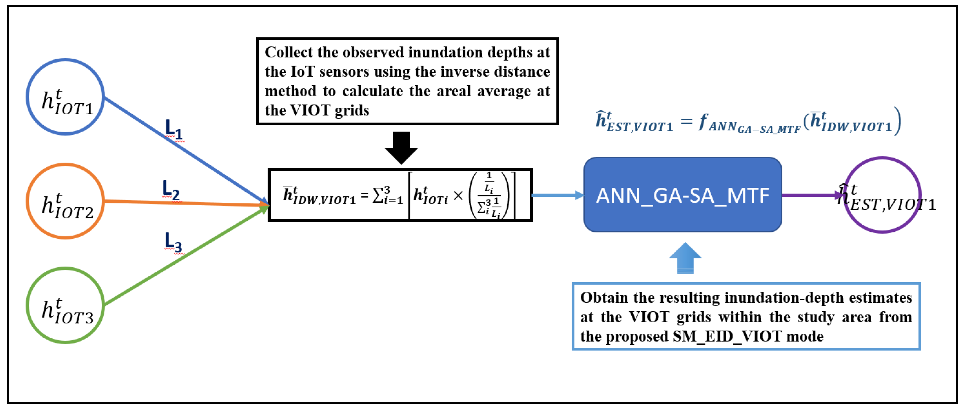
In this study, deriving the SM_EID_VIOT model, the inundation depths at the VIOT spots are first estimated by the geostatistical approach (i.e., the inverse distance method) treated as the spatial average ${\overline{h}}_{IDW,VIOT}^t$ using the following equation:

$${\overline{h}}_{IDW, VIOT=}^t{{\displaystyle \sum }}_{i=1}^3\left[h_{IOTi}^t\times \left(\frac{\frac{1}{L_i}}{{{\displaystyle \sum }}_i^3\frac{1}{L_i}}\right)\right]$$

(6)

where $h_{IOTi}^t$ and L_i stand for the observed inundation depth at the ith IoT sensor and associated distance to the virtual IoT grids (VIOT), respectively; the equations of the estimated inundation depths at the VIOT grids with the observations at the roadside IoT sensors are then established based on the ANN_GA-SA_MTF model; namely, the ANN_GA-SA_MTF model derived can be regarded as an equation for adjusting the estimated spatial averages of the inundation depths at the specific VIOT grids (${\overline{h}}_{IDW, VIOT1}^t$) to be the corresponding inundation-depth estimates (${\widehat{h}}_{EST,VIOT1}^t$) as follows:

$${\widehat{h}}_{EST,VIOT1}^t=f_{AN{N}_{GA-SA\_MTF}}({\overline{h}}_{IDW,VIOT1}^t)$$

(7)

Figure 3 presents the graphical process of calculating the average of the IoT-related inundation depths as the model inputs for the ANN_GA-SA_MTF model to estimate the inundation depths at the VIOT grids within the proposed SM_EID_VIOT model.

2.5. Integration with Real-Time Correction Approach

Despite the proposed SM_EID_VIOT model providing the more reliable inundation depths at the VIOT grids using the ANN_GA-SA_MTF model, the accuracy of the resulting inundation depths at the ungauged locations and corresponding flooding area are probably impacted due to the uncertainties in the parameters of the ANN_GA-SA_MTF model (i.e., ANN weights); also, in referring to Equation (6), the correlation between the estimated inundation depths at the VIOT grids and observation at the roadside IoT sensors might decline with their distances from the VIOT spots, accounting for the less accurate inundation-depths from the proposed SM_EID_VIOT model would be obtained at the VIOT spots further away from the IoT sensors. Therefore, to boost the accuracy of the estimated inundation depths at the VIOT grids, the proposed SM_EID_VIOT model collaborates with the real-time error correction method for the 2D inundation simulation (named RTEC_2DIS) [2].

The RTEC_2DIS model has two steps: at-site correction and regional correction. With respect to the at-site correction, the water-level error at the current time $t^{*}$ and $t^{*}+1$ estimated equations are derived through the time-series approach and Kalman filtering algorithm (name RTEC_TS&KF) [27], respectively:

$${\epsilon }_{corr}^{t^{*}}=h_{obs}^{t^{*}}-h_{est}^{t^{*}}$$

(8)

$${\epsilon }_{corr}^{t^{*}+1}={\epsilon }_{TS}^{t^{*}+1}+{\epsilon }_{KF}^{t^{*}+1}$$

(9)

where $h_{obs}^{t^{*}}$ and $h_{est}^{t^{*}}$ stand for the observed and estimated water level at the current time $t^{*}$, respectively; and ${\epsilon }_{TS}^{t_{pred}} and {\epsilon }_{KF}^{t_{pred}}$ serve as the forecast error estimated by the time series approaches and Kalman filtering method, respectively; after that, within the regional-correction step, the corresponding water-level errors at the ungauged locations can be quantified using the Kriging equation with the weighted semivariogram functions [28,29].

Within the adjustment of the inundation–depth estimates at the VIOT grids using the RTEC_2DIS algorithm, the spatial averages (${\overline{h}}_{IOT}^t$) of the estimated inundation depths $h_{VIOTi}^{t^{*}}$) by the proposed SM_EID_VIOT model at the four VIOT grids around the specific IoT sensors are treated as the corresponding simulations via the following equation:

$${\overline{h}}_{IOT}^t=\frac{1}{4}{\displaystyle \sum }_1^4{h}_{VIOTi}^t$$

(10)

Thus, the corresponding errors at the IoT sensors could be quantified based on the difference between the simulations and observations at the previous time steps during the rainstorm using Equations (8) and (9). Since the proposed SM_EID_VIOT model estimates the inundation depths at the VIOT grids with the measurements at the road IoT sensors, the errors of the estimated inundation depths at the current time are considered in quantifying the error of the inundation-depth estimates at the VIOT grids within the regional error correction. Eventually, the correction of the VIOT-related inundation depths estimated via the proposed SM_EID_VIOT model can be achieved by the following equation:

$$h_{Corr, VIOTi}^t=h_{Est, VIOTi}^t+{\epsilon }_{corr,VIOTi}^{t^{*}}$$

(11)

where $h_{Est, VIOTi}^t$ is the estimated inundation depth at the ith VIOT grid regarding the current time step t; $h_{Est, VIOTi}^t$ is the estimated error of the inundation-depth estimate at the ith VIOT grid by the RTEC_2DIS method; and $h_{Corr, VIOTi}^t$ denotes the corrected inundation-depth estimate at the ith VIOT grid.

2.6. Model Framework

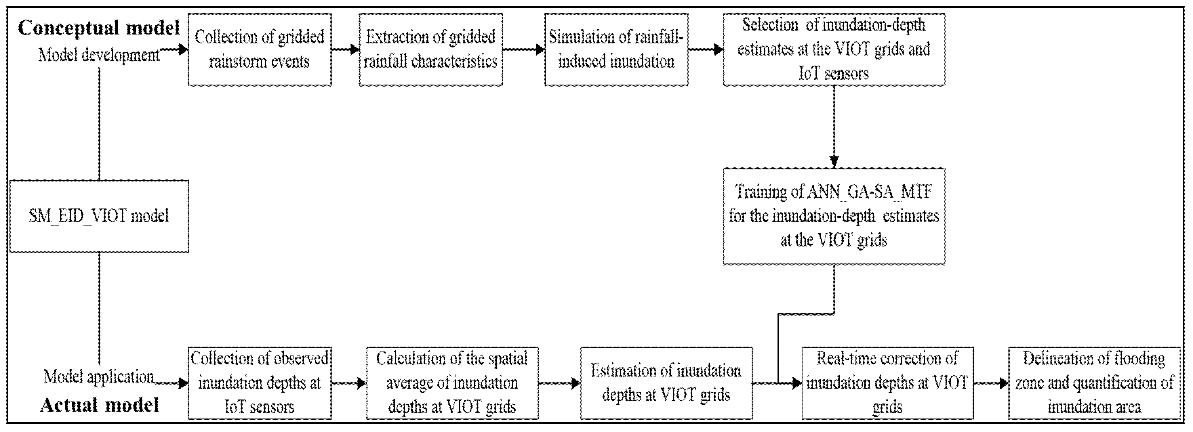
To sum up the introduction to the concepts mentioned above, the development and application of the proposed SM_EID_VIOT model can be classified into five parts: (1) generation of the rainstorm events at all grids within the study area; (2) 2D rainfall-induced inundation simulations; (3) Identification of the ungauged grids as the virtual IoT (VIOT) grids; (4) Training of the ANN_GA-SA_MTF model in the estimation of the inundation depths at the VIOT grids; and (5) Integration with the 2D real-time error correction model for the 2D inundation simulation. Note that the proposed SM_EID_VIOT model can be separated into two parts: the conceptual and actual models. In detail, the proposed SM_GA-SA_MTF model developed can be regarded as the conceptual model for training the ANN-GA-SA_MTF model using the simulations of rainfall-induced flood events obtained by the SOBEK with the generated rainstorms. Then, the proposed SM_EID_VIOT model can be treated as an actual model in which the resulting ANN-GA-SA_MTF model can be applied in the estimation of the ungauged locations. The detained framework of the model development (conceptual model) and application (actual model) are addressed as follows:

2.6.1. Conceptual Model

Step 1: Collect the gridded hyetographs of historical rainstorm events within the study area and extract their gridded characteristics, i.e., rainfall duration, gridded rainfall depth, the areal average of the cumulative dimensionless rainfall, and the associated bias;

Step 2: Generate a significant number of rainfall fields with high spatiotemporal resolutions comprised of the simulated gridded rainfall characteristics by the SM_GSTR model with the statistical properties of gridded rainfall characteristics extracted at Step [1].

Step 3: Perform the 2D inundation simulation using the SOBEK model with the numerous gridded rainstorms simulated at Step 2 to obtain the simulations of inundation depths at all the grids, including the VIOT grids and IoT sensors.

Step 4: Recognize the inundated grids defined as the virtual (VIOT) grids associated with the probabilities of the corresponding nonzero inundation depths at all the grids from a great number of rainfall-induced rainfall flood events.

Step 5: Extract inundation-depth estimates regarding the specific time steps during the simulated flood events at the VIOT grids and IoT sensors regarding the particular time steps.

Step 6: Calculate the spatial average of inundation-depth estimates obtained in Step 5 at the roadside IoT sensors through Equation (6) as the model inputs of the ANN_GA-SA_MTF at the VIOT grids, where the corresponding simulations of the inundation depth are treated as the model outputs.

Step 7: With the model inputs and outputs summarized in Step 6, training the ANN_GA-SA_MTF model regarding the VIOT grids to determine the associated ANN-related coefficients as the parameters of the SM_EID_VIOT model.

2.6.2. Actual Model

Step 1: Collect the observed inundation depths during the rainfall-induced flood events at the IoT sensors using the inverse distance method to calculate the areal average at the VIOT grids of interest, as shown in Figure 4.

Step 2: Obtain the resulting inundation-depth estimates at the VIOT grids within the study area from the proposed SM_EID_VIOT model.

Step 3: Compute the averages of the inundation-depth estimates at the four VIOT grids around the IoT sensors of interest as the corresponding estimations via Equation (9).

Step 4: Carry out the real-time correction for the resulting inundation-depth estimates at all the VIOT grids from the proposed SM_EID_VIOT model coupled with the RTEC_2DIS method based on the bias of the inundation-depth estimates in comparison to the measurements at the IoT sensors obtained in Step 4.

Step 5: Delineate the flooding zone according to the corrected inundation-depth estimates at all VIOT grids and summarize the number of the inundated VIOT grids to quantify the flooding area. The framework for the model development and application regarding the proposed SM_EID_VIOT can be referred to in Figure 4.

3. Study Area and Data

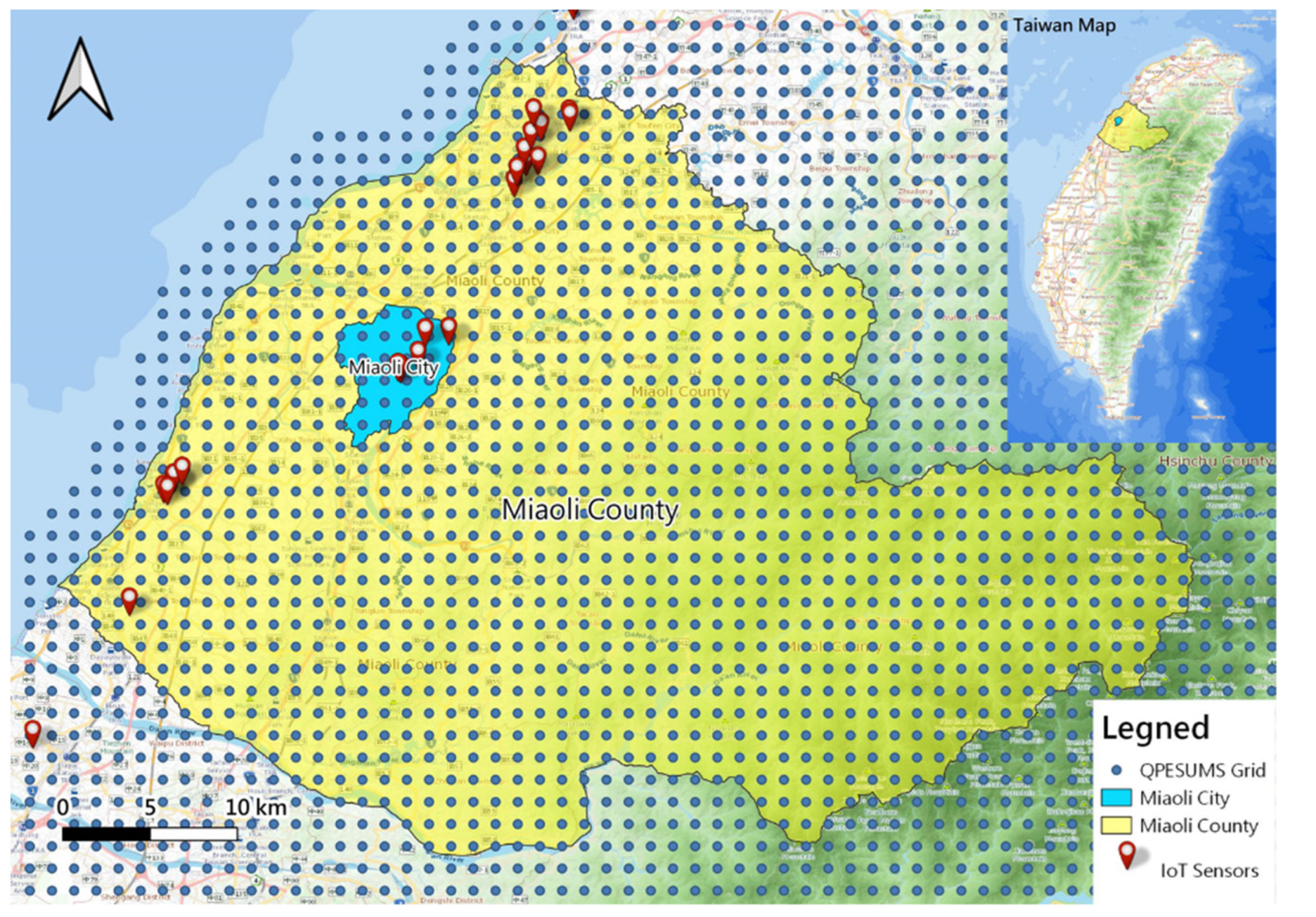
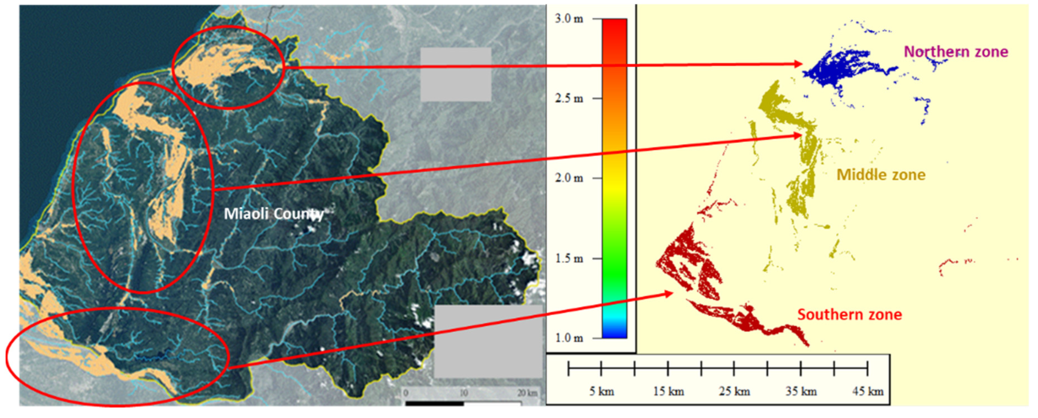
Miaoli County is a county in western Taiwan adjacent to Hsinchu County and Hsinchu City to the north, Taichung to the south, and borders the Taiwan Strait to the west (see Figure 5). Miaoli County comprises the eighteen townships in which Miaoli City, selected as the study area, is the county’s capital. Of the main neighboring rivers within Miaoli County, including the Houlong River and Zhonggang River, the Houlong River is the biggest one in Miaoli County, of which the watershed area and length are approximately 537 km² and 58.3 km, respectively.

Within Miaoli County, various hydrological measurement sites have been set up, including 65 rain-gauges, three water-level stations, and two reservoirs (Min-Te and Liyu-Lake). Note that the 22 roadside IoT sensors, whose symbol is the redpoint (see Figure 5), immediately detect the inundation depths through the internet of Things (IoT) technique configured in Miaoli City. In addition to the hydrological measurement sites, the 1045 radar-precipitation grids (symbolled as the blue circles) with a high resolution in time (15 min) and space $\left(1.5\mathrm{km}\times 1.5\mathrm{km}\right)$ provided by the Taiwan Central Weather Bureau (CWB), the 22 radar-precipitation grids of which are located in the Miaoli City. In this study, the 50 rainstorm events recorded from 2009 to 2018 are utilized to simulate the rainfall-induced inundation as the training and validating datasets for the proposed SM_EID_VIOT model.

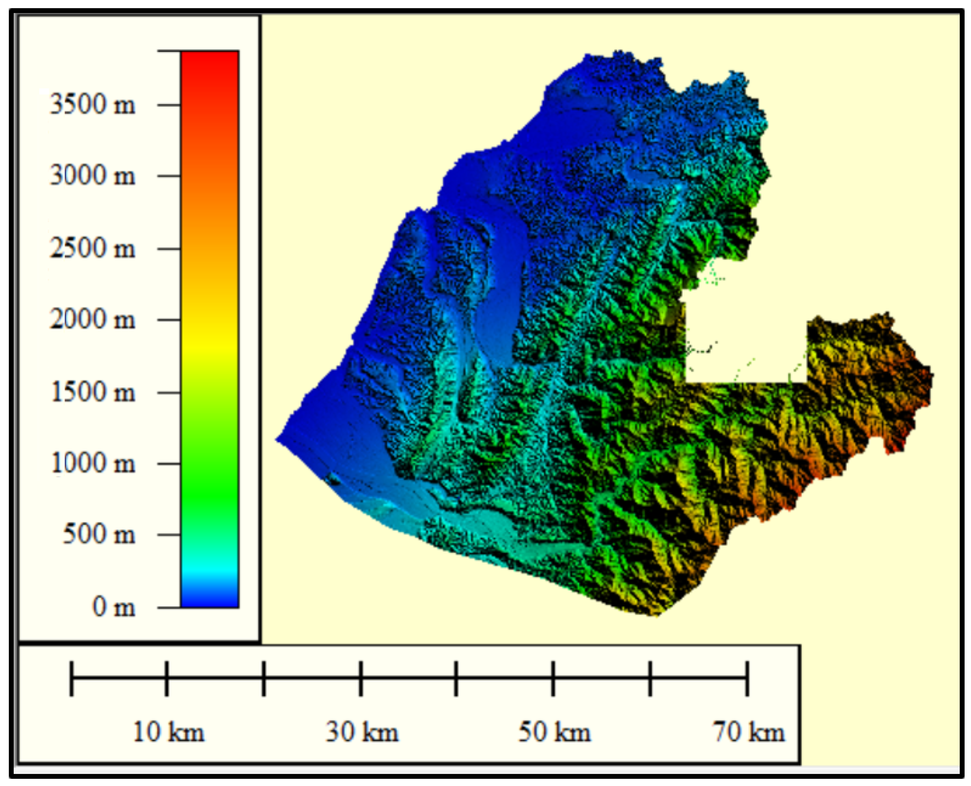
In addition to the gridded rainstorms, the topographical data are supposed to be required in the hydraulic modeling, of which the topographical information, the digital elevation map (DEM), is comprehensively used for describing the flow paths triggered by flood events so that the DEM within in Miaoli County (see Figure 6) is applied in the 2D inundation simulation. In Figure 6, it can be seen that the west of Miaoli County is the plain region, and the other side is an alpine zone, meaning that apparent variation exists in the elevation within Miaoli County.

4. Results and Discussions

4.1. Simulation of Rainfall-Induced Inundation

4.1.1. Extraction of Gridded Rainstorms

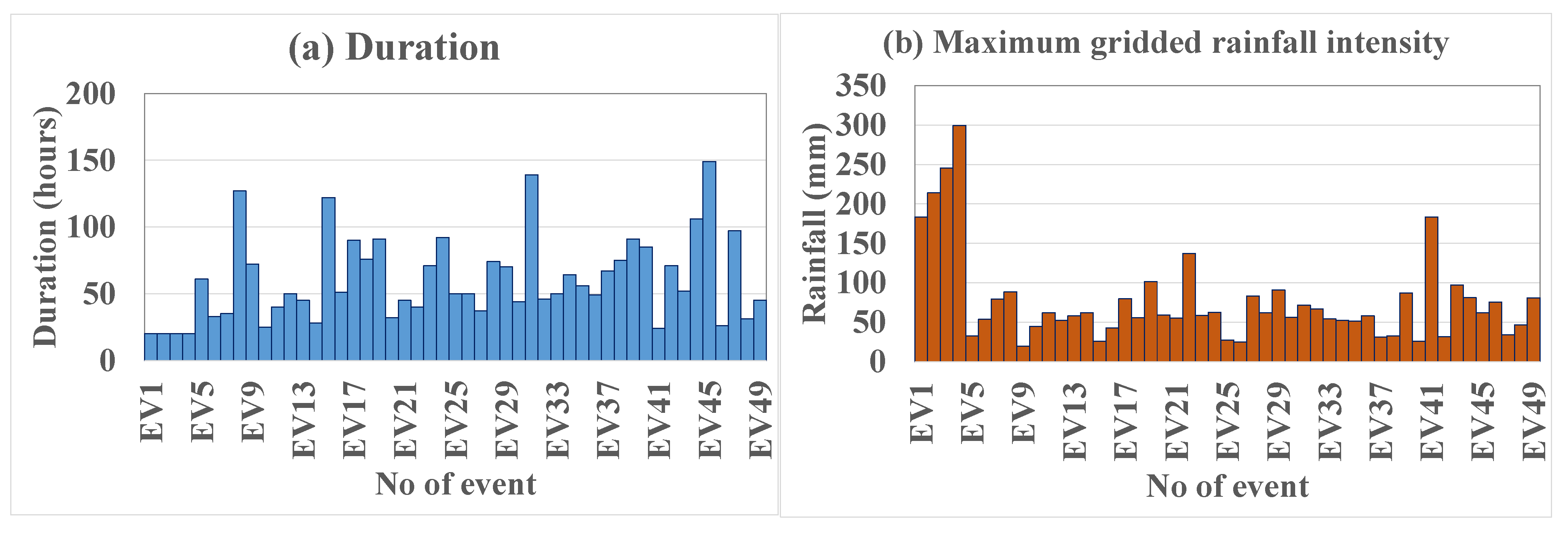
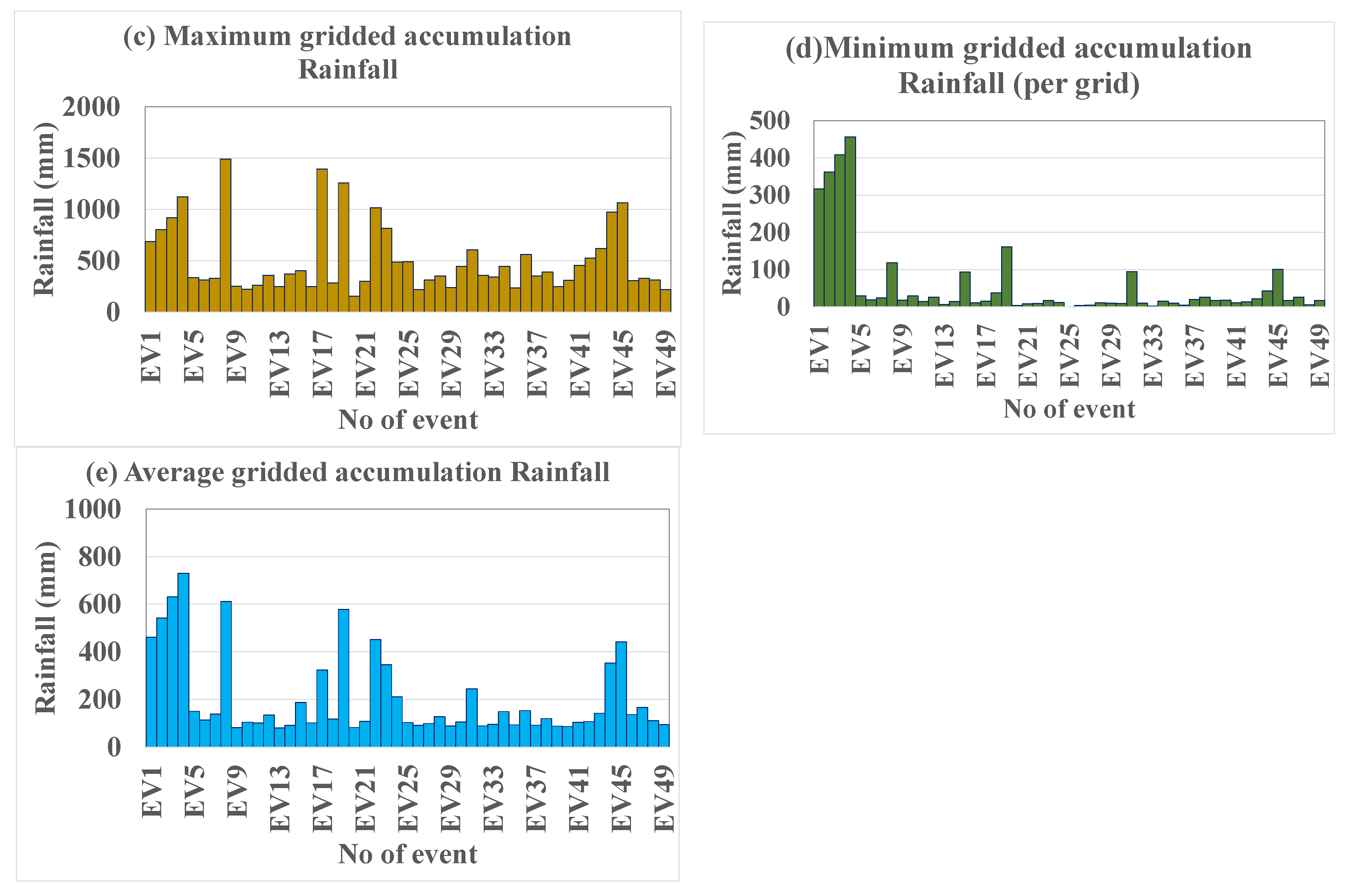
Before carrying out the rainfall-induced inundation in the model development, as shown in Figure 5, the gridded rainfall characteristics should be extracted from the 50 historical events (see Figure 7), meaning that the maximum and minimum duration of historical rainstorms of interest are approximate 149 h and 20 h, respectively, with the average of 60 h; the maximum gridded rainfall depths in space at each time step are located between 5 mm and 1490 mm associated with a spatial average ranging from 100 to 800 mm; additionally, the maximum of the rainfall intensity regarding 50 events, on average, approximates 77 mm/h, with a significant variance coefficient of 0.75. In summary, it can be said that the various storm patterns, the distribution of rainfall in time, can be recognized, implying a variety of the rainstorms with significantly different spatial and temporal variations in Miaoli County.

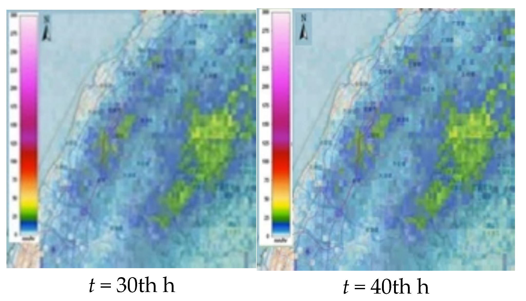
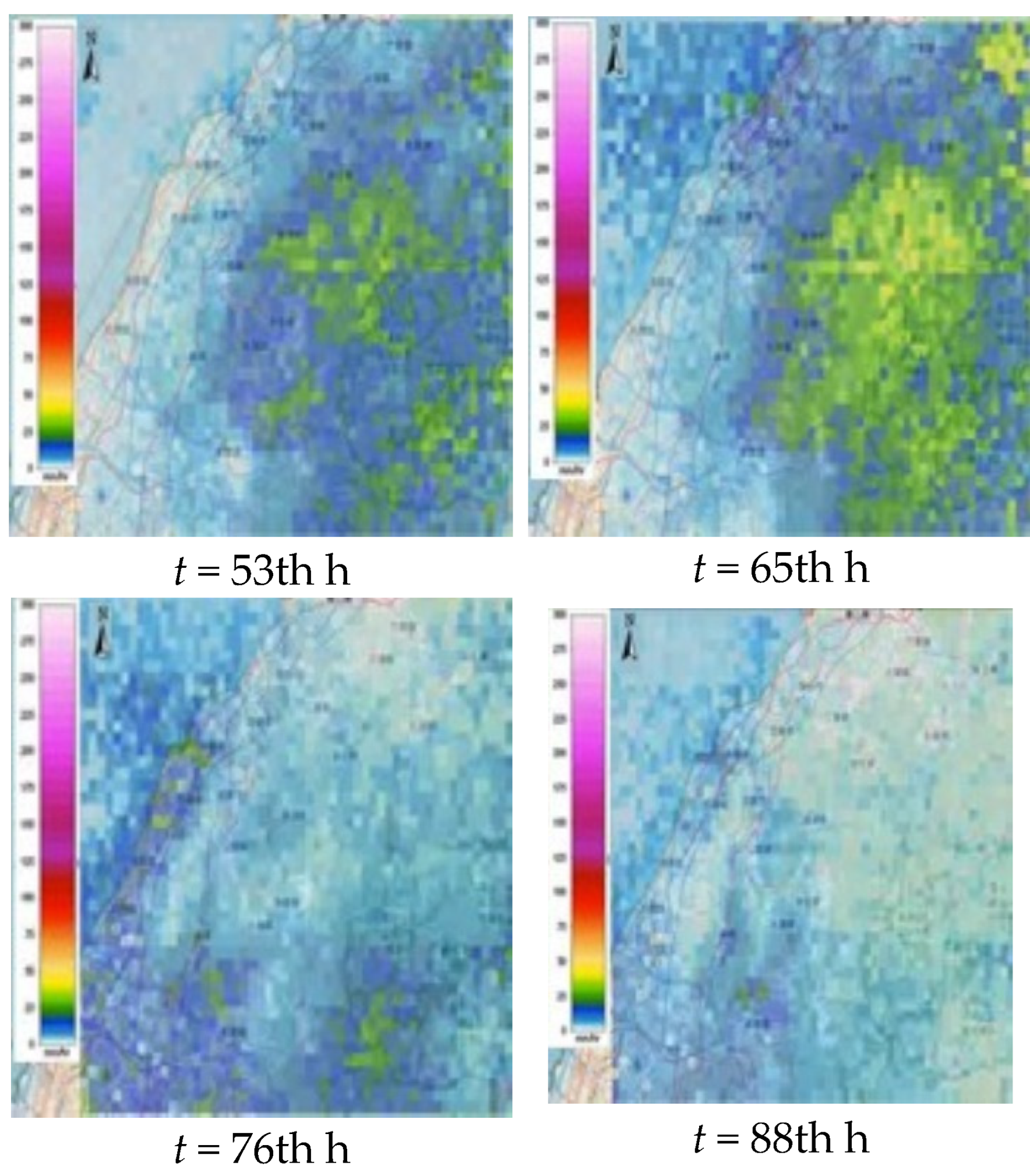
Using the SG_GSTR model with the statistical features of the gridded rainfall characteristics, the 1000 simulations of the rain fields consisting of the simulated gridded rainfall characteristics can be obtained. Figure 8 presents the varying trend of the simulated rainstorm of 101 h at all grids in time, showing that the simulated rainstorm realistically moves from the ocean beach (East) to the Mountain zone (West) within the study area (Miaoli County). The maximum rainfall occurs near the mountain zone, apparently in response to the gridded rainfall characteristics in Miaoli County.

4.1.2. Simulation of Rainfall-Induced Inundation Events

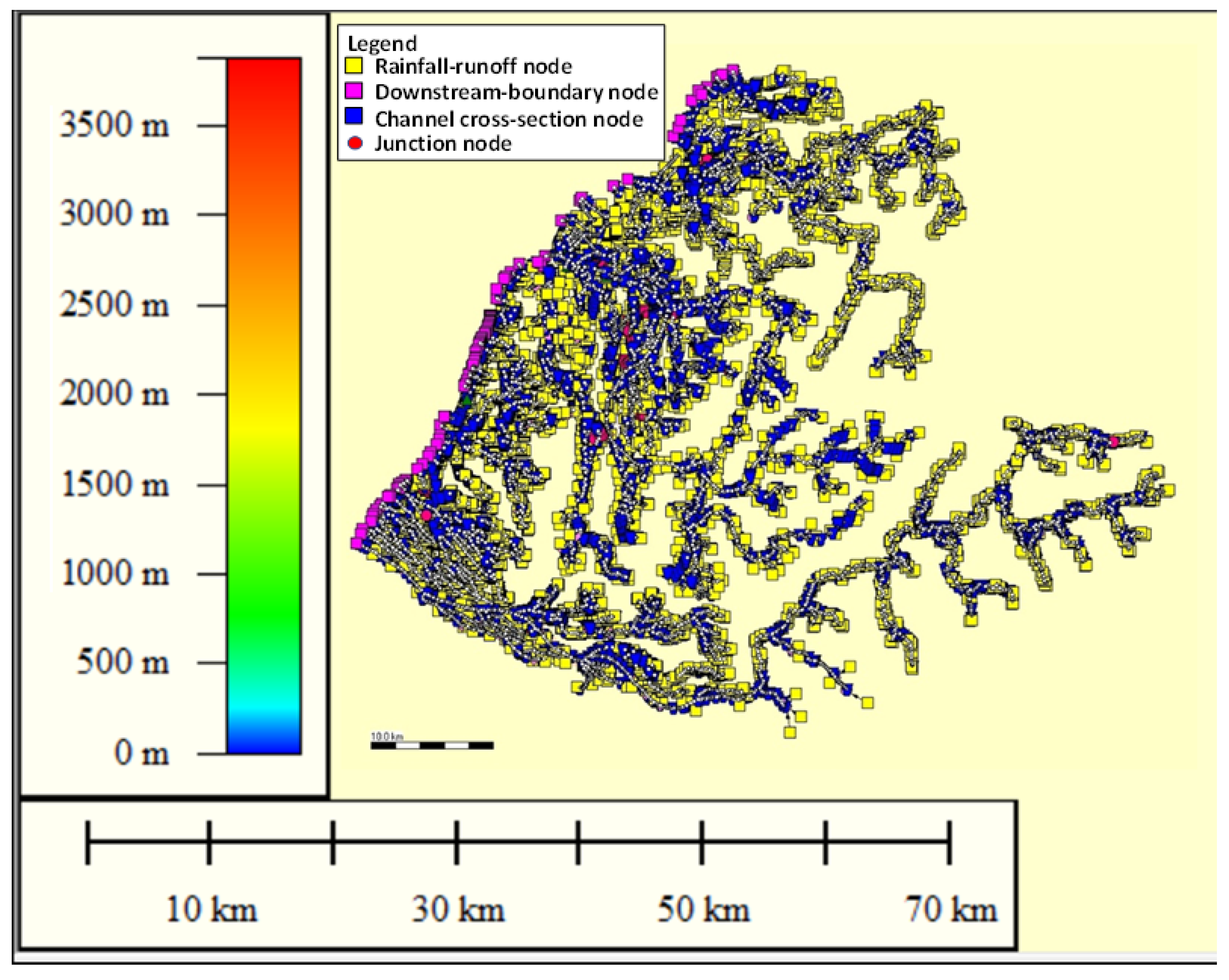
This study employs the SOBEK 1D-2D hydrodynamic model to implement the inundation simulation with 40 m $\times 40$ m DEM (see Figure 6). In addition to the DEM of Miaoli County, a variety of hydraulic structures, such as the drainage channel, the pumping stations, sewer system, and draining gates, are required in seeking to configure the 2D inundation simulation model;

Table 3. Summary of computation objects adopted in the SOBEK model regarding Miaoli County.

Function	Facilities	Number
Hydraulic analysis	Sub-basins	4731
	Cross-sections	9838
	Gates	62
	Bridges	9018
	Sewer	68.6 km
	Maintenance of sewer system	1382
Hydrological analysis	Rainfall-runoff node	4097

lists the computation objects, simulating the hydrological and hydraulic analysis, adopted in the configuration of the 2D SOBEK regarding Miaoli County. Furthermore, in the resulting SOBEK model, rainfall-induced runoff is quantified via rainfall-runoff models (e.g., SCS-UH and SAC-SMA). Consequently, Figure 9 shows the river-channel network and the computation objects (as listed in Table 3) set up in the SOBEK model based on the DEM of Miaoli County.

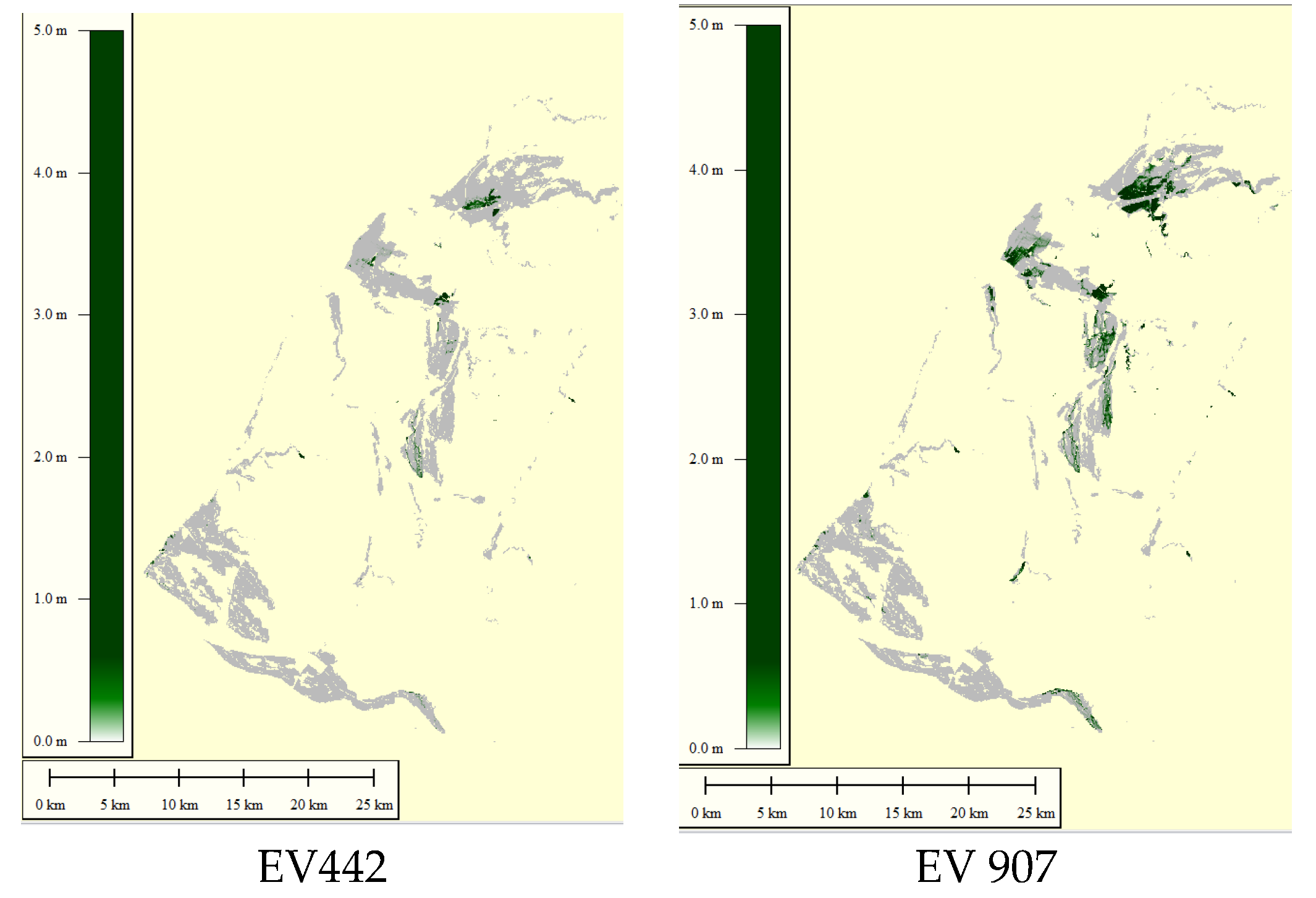
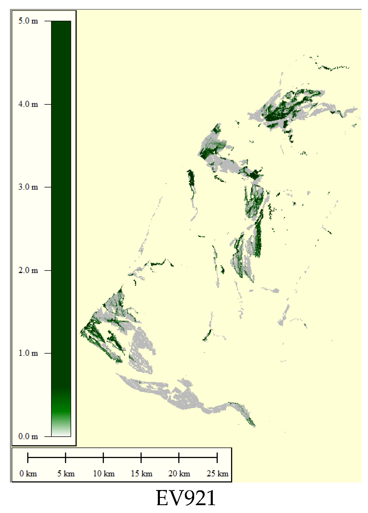
Finally, using the SOBEK model derived for Miaoli County with the 1000 simulations of the gridded rainstorm events, the resulting 2D inundation simulations, including the gridded inundation depths and corresponding flooding area, could be accordingly reproduced. Figure 10 illustrates the simulated flooding areas drawn based on the maximum inundation depths for three simulated rainfall-induced flood events (i.e., EV402, EV907, and EV921), indicating that the flooding regions in Miaoli County could be briefly grouped into the three zones, including the Northern, Middle and Southern zones as shown in Figure 11. Since Miaoli City is the capital of Miaoli County near the Middle zone, this study selects Miaoli City as the primary study area where the model development and validation regarding the proposed SM_EID_VIOT would be achieved.

4.2. Identification of Ungauged Locations as VIOT Grids

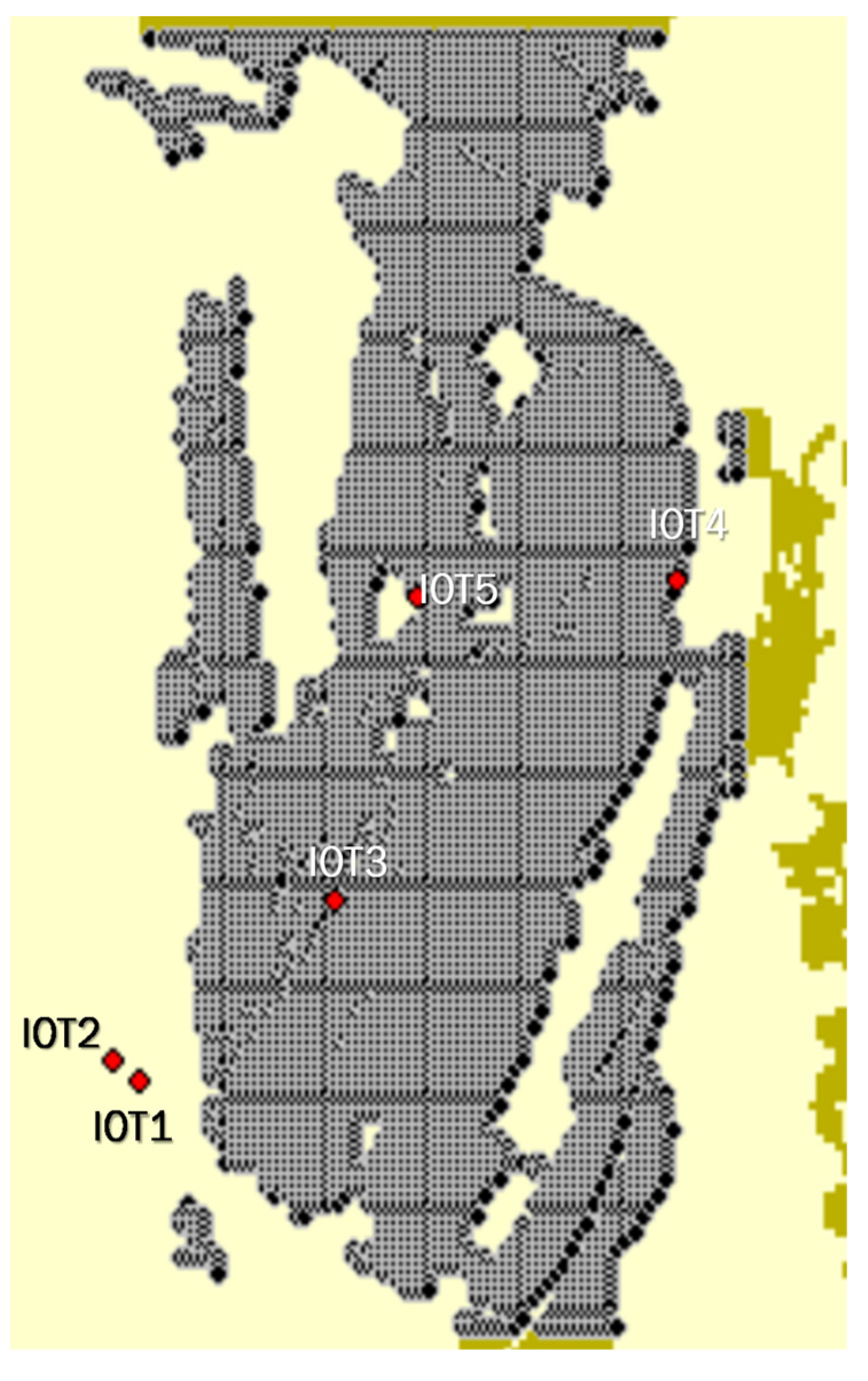
According to the framework of developing the proposed SM_EID_VIOT model, the ungauged locations are treated as the VIOT grids based on the results from the simulated grid-based inundation depths within the study area; the flooding risk at all the grids in the study area Miaoli City can be quantified through Equation (3) in terms of the probability of the inundated grids ($P_f\left(h_f>0\right)$) as shown in Figure 12, involving the five IoT sensors. As a result, it can be known that the 6823 ungauged locations can be defined as the VIOT grids (symbolized as the white points); additionally, among the five roadside IoT sensors, IOT3, IOT4 and IOT5 sit within the VIOT grids.

4.3. Training of ANN-Derived Model

Based on the model-development framework, the proposed SM_EID_VIOT model in estimating the inundation depths at VIOT is derived by calibrating the parameters of the ANN_GA-SA_MTF model with the model inputs and outputs related to the estimated inundation depths at the 6823 VIOT grids and three roadside IoT sensors. In detail, when developing the SM_EID_VIOT model for the 6823 VIOT grid, as shown in Figure 12, the simulations of inundation depths at the IoT3-IoT5 sensors are extracted in advance to calculate their average corresponding to the VIOT grids through Equation (6) as the model inputs of the ANN_GA-SA_MTF model; whereas, the corresponding simulated inundation depths at the VIOT grids are then treated as the model output. It should be noted that the parameters of the ANN_GA-SA_MTF model can be calibrated for each VIOT grid; namely, the VIOT grids have their parameters of the ANN_GA-SA_MTF. Therefore, the 6823 sets of the ANN_GA-SA_MTF-appropriate parameters are supposed to be determined for the SM_EID_VIOT model for the study area Miao City.

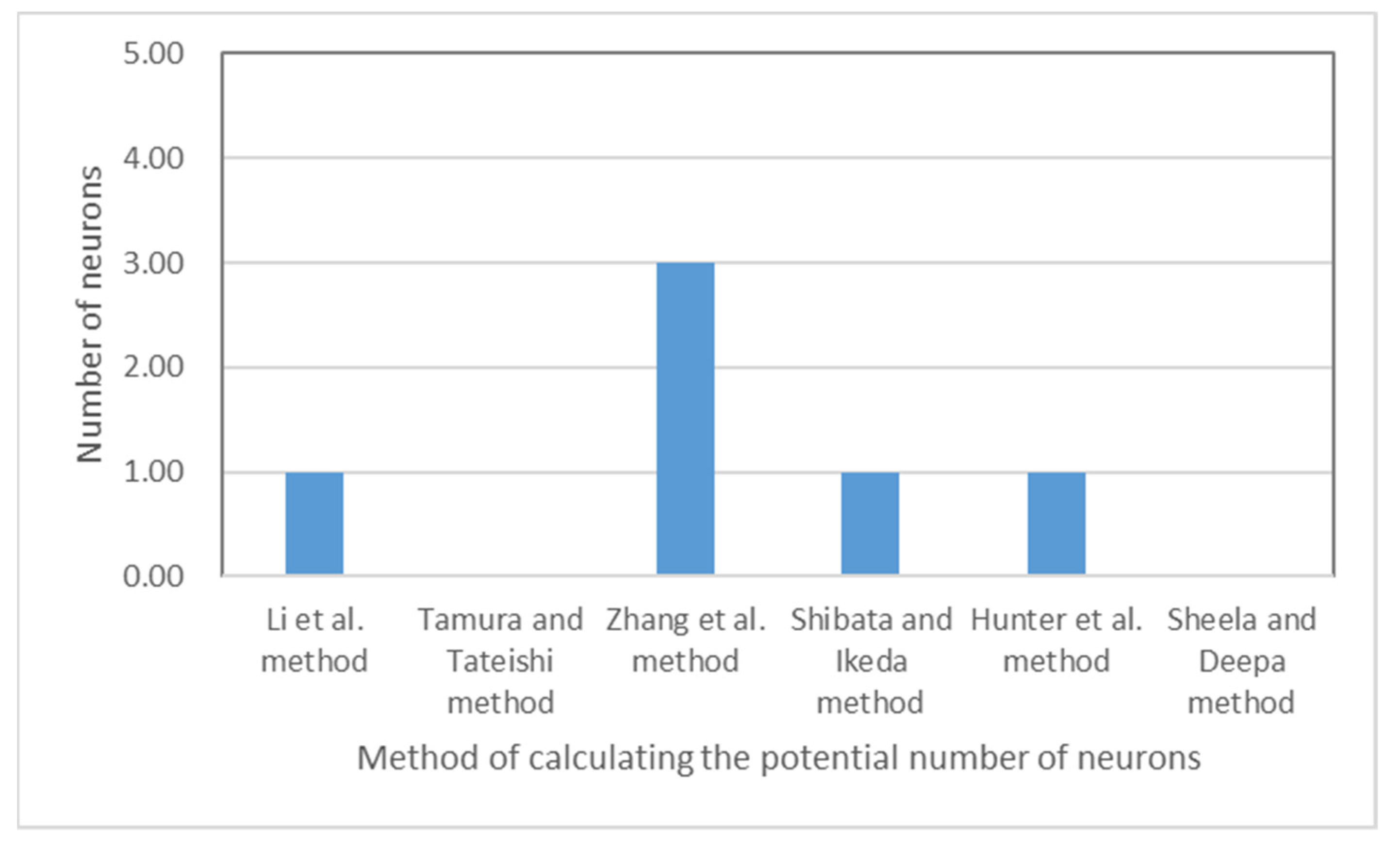
When training the ANN-derived models, the initial conditions, including the number of hidden layers, the total number of neurons, and transfer functions of interest (see Table 2), should be given in advance. It is well-known that the 3-layer network structure: one input layer, one output layer, and one hidden layer, is frequently utilized in hydrological/hydraulic modeling [1,14]; thus, the proposed SM_EID_VIOT model is developed using the 3-layer ANN_GA-SA_MTF model. Additionally, the number of neurons can be estimated via the numerous formulae (see Table 1) with the number of model inputs and outputs. Figure 13 shows the resulting number of neurons from the different equations ranging from one to three, implying that the three neurons are suitable for exhibiting the nonlinear relationship between the inundation depths at the VIOT grids and roadside IoT sensors. Concerning the remaining parameters, e.g., the statistical moments of ANN weights and bias and adjustment factor, their initial conditions can be considered in

Table 4. Settings of the proposed ANN-GA-SA_MTF model.

Parameters	Definition
Transfer functions used	TF1-TF10
Input factors	Resulting areal average of Inundation depth from IoT sensors	${\overline{h}}_{IDW,VIOT1}^t$
Output factor	Inundation depth at VIOT grids	${\widehat{h}}_{EST,VIOT1}^t$
Number of hidden levels	1
Number of neurons	3
Calibration of parameters of transfer function	Number of optimizations	10
	$\mathrm{Weights}\mathrm{of}\mathrm{neurons}({\mathsf{\omega }}_{HL})$	Mean	1
		Standard deviation	3
	$\mathrm{Bias}\mathrm{of}\mathrm{function}({\mathsf{\theta }}_{TF})$	Mean	0
		Standard deviation	1
	$\mathrm{Adjusting}\mathrm{factor}({\propto }_{TF})$	Mean	1
		Standard deviation	0.005

.

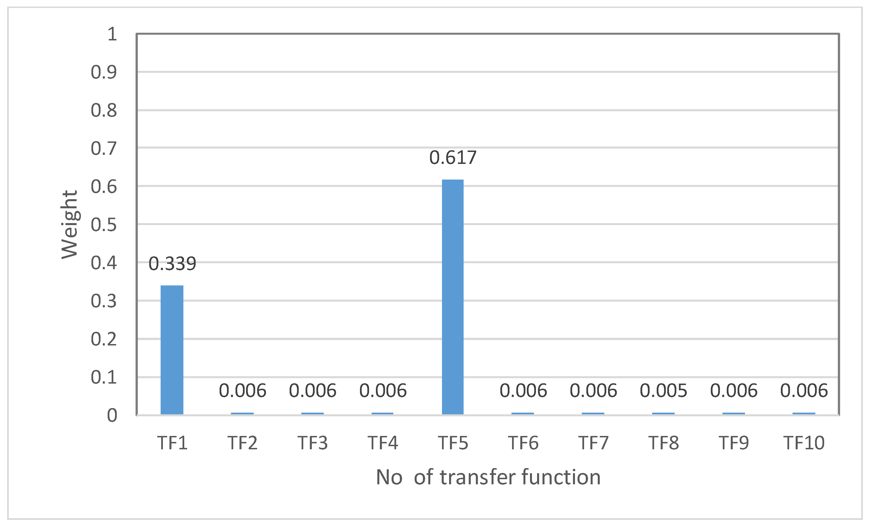
Using the parameter definition shown in

Table 5. Summary for the appropriate calibrated parameters of the ANN_GA-SA_MTF model at the 500th VIOT grid.

Transfer Function	No of Optimization	Adjust Factor $\left({\propto }_{\mathit{T}\mathit{F}}\right)$	1.00113
1	OPT1	Weights of $\mathrm{neurons}{\omega }_{HL}$	The 1st hidden layer		Input factors
					1	Bias
			Neuron	1	2.27251	−1.14272
				2	0.58986	−2.71961
				3	4.56974	−4.28293
			Output layer		The 1st hidden layer
					1	2	3	Bias
			Input factor	1	−0.87316	1.04999	0.08291	−0.21039

, the SM_EID_VIOT model can be developed by training the ANN_GA-SA_MTF model with the simulations of the inundation depths regarding the specific time steps, equal to the ratio of 0.3, 0.4, 0.5, 0.7, 0.8 and 0.9 multiplied by duration, at the IoT sensors and the VIOT grids, extracted from 1000 rainfall-induced inundation-simulation datasets. Table 5 summarizes the appropriate parameters of the ANN_GA-SA_MTF model calibrated using the transfer function TF1 (Sigmoid function). Additionally, Figure 14 presents the weighted factors of the transfer functions used for calculating the weighted average of the resulting inundation-depth estimates from various transfer functions, indicating that the various transfer functions with the different scales of the weighted factors significantly contribute to the estimation of the inundation depths at the VIOT grids. Among the transfer functions, the TF1 and TF5 contribute to estimating the inundation depths at the 500th VIOT grid due to the extensive weights, 0.33(TF1) and 0.62 (TF6), respectively.

$\mathrm{neurons}{\omega }_{HL}$ Consequently, within the ANN_GA-SA_MTF model for the estimated inundation depths at the VIOT grids, uncertainty in the formulation of the transfer functions on the estimation of model outputs can be effectively reduced by computing the corresponding weighted average of the results from the multiple transfer functions. Since the 6823 VIOT grids are recognized in the study area Miaoli City, the 6823 sets of the appropriate parameters of the ANN_GA-SA_MTF models should be determined; Table 5 illustrates the results from the parameter calibration of the ANN_GA-SA_MTF model for the 500th VIOT grid, the location (TWD97_X: 231658.5, TWD97_Y: 271841).

4.4. Model Validation

To demonstrate the reliability and accuracy of the proposed SM_EID_VIOT model, its performance could be made in comparison to the inundation depths at the ungauged locations (i.e., VIOT grids) and corresponding flooding area. In theory, the accuracy and reliability of the results from the proposed model should be compared with the observations. However, flooding merely taking place the Miaoli City leads to few inundation depths observed at the IoT sensors considered. Thereby, a simulated rainfall-induced inundation event, i.e., the 921st simulated rainstorm event of 51 h, in which the associated simulations of the inundation-depth and flood-area hydrographs would be applied in the model development and validation.

4.4.1. Extraction of Validation Data

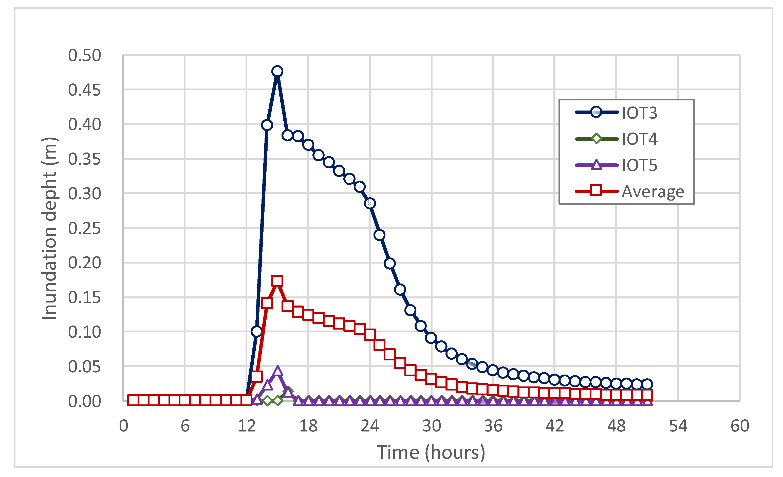
Since the proposed SM_EID_VIOT model estimates the inundation depths at the ungauged locations (i.e., VIOT grids) based on the measurements at the roadside IoT sensors, the inundation-depth estimates at the roadside IoT sensors should be extracted from the training data as shown in Figure 15 and Figure 16 (named the validated data). From Figure 15, it can be known that inundation obviously occurs from t = 13-h, meaning that the inundation-depth estimates at the IoT4-5 are 0 m between t = 1-h and 12-h; whereas the inundation-depth estimates increase with time and reach the maximum values, 0.47 m (IOT3), 0.04 m (IOT5) at t = 15-h; then, they generally decline to 0.02 m (ITO3) and 0.0002 m (IOT4 and IOT5) from t = 16-h to t = 51-h.

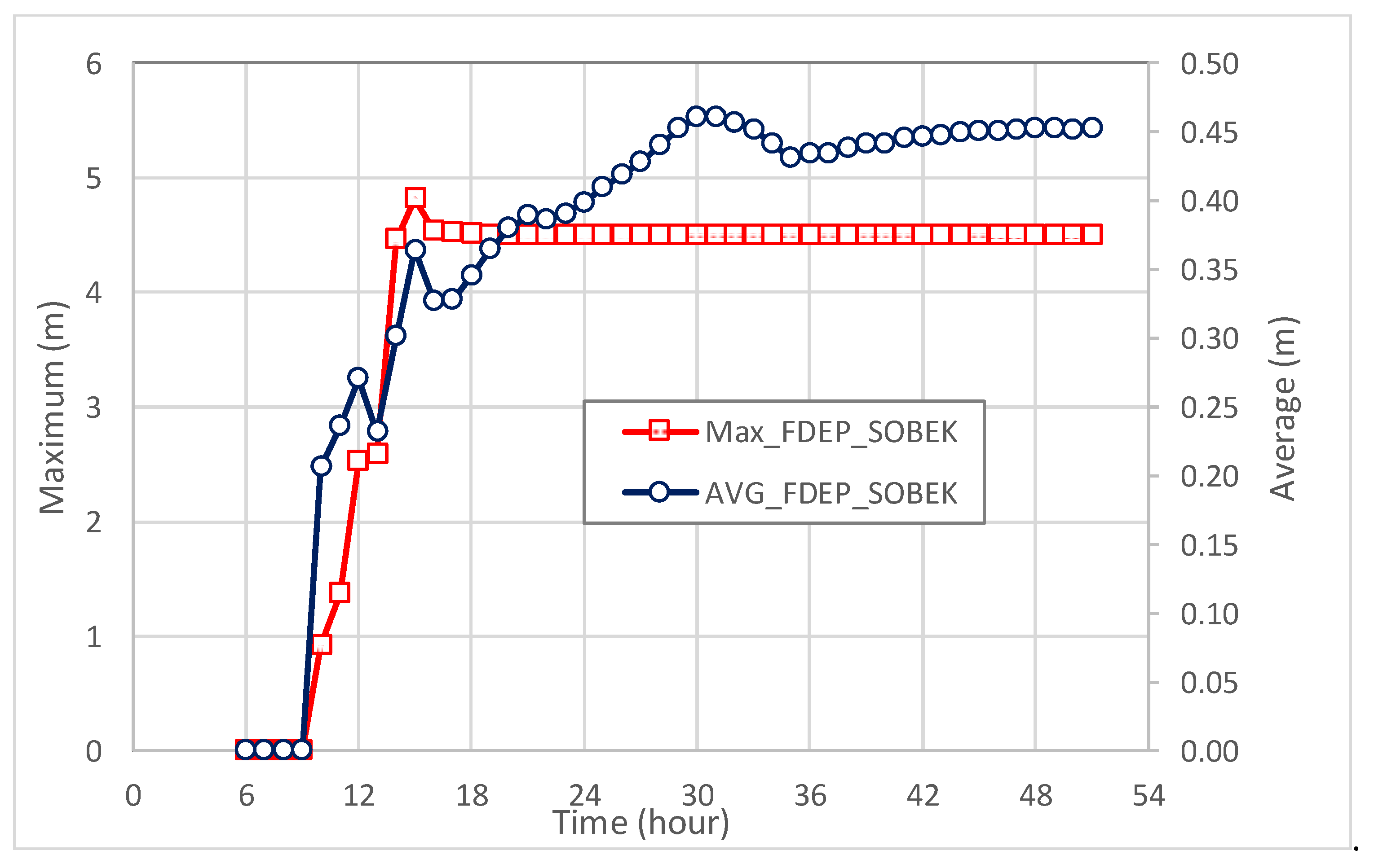
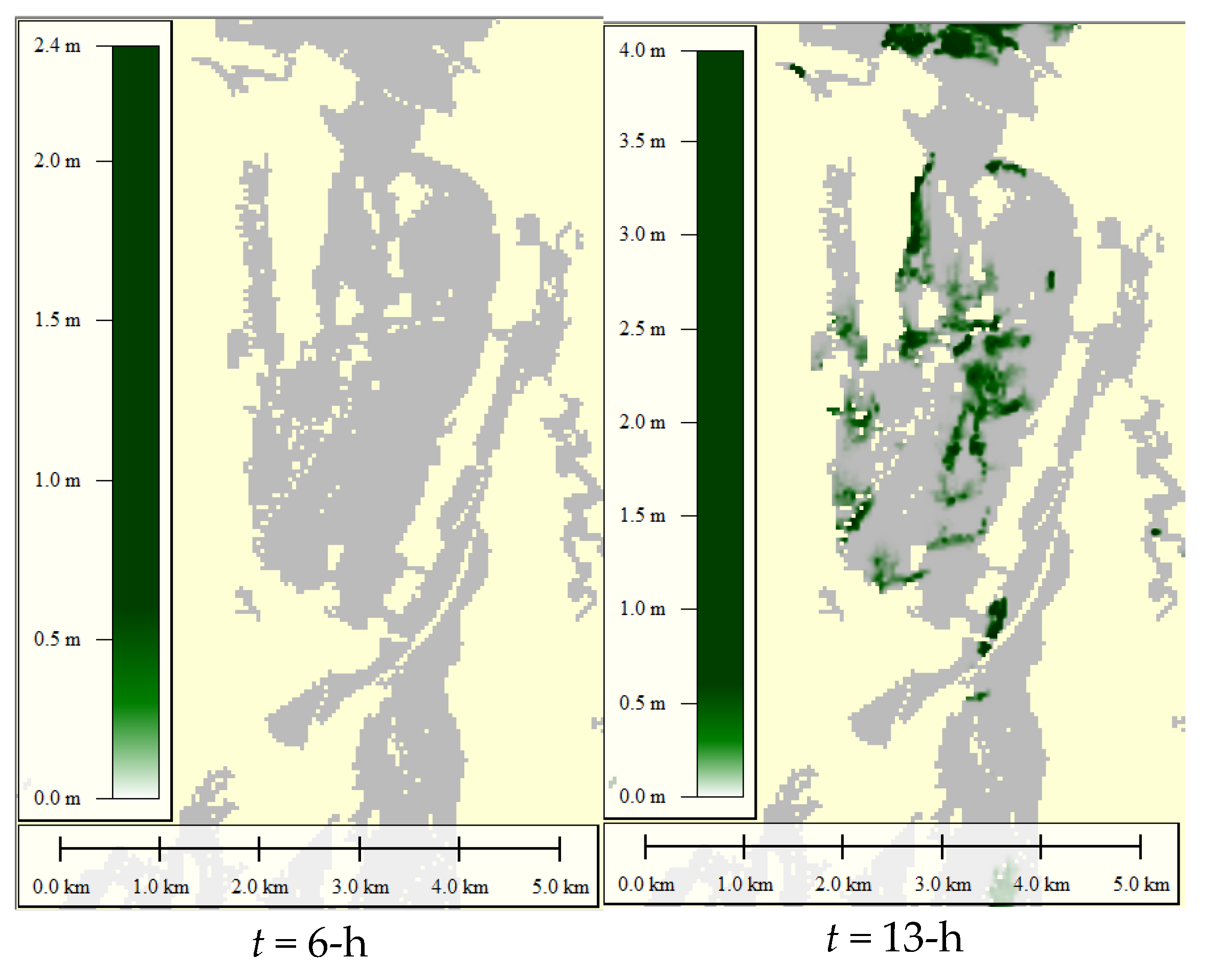
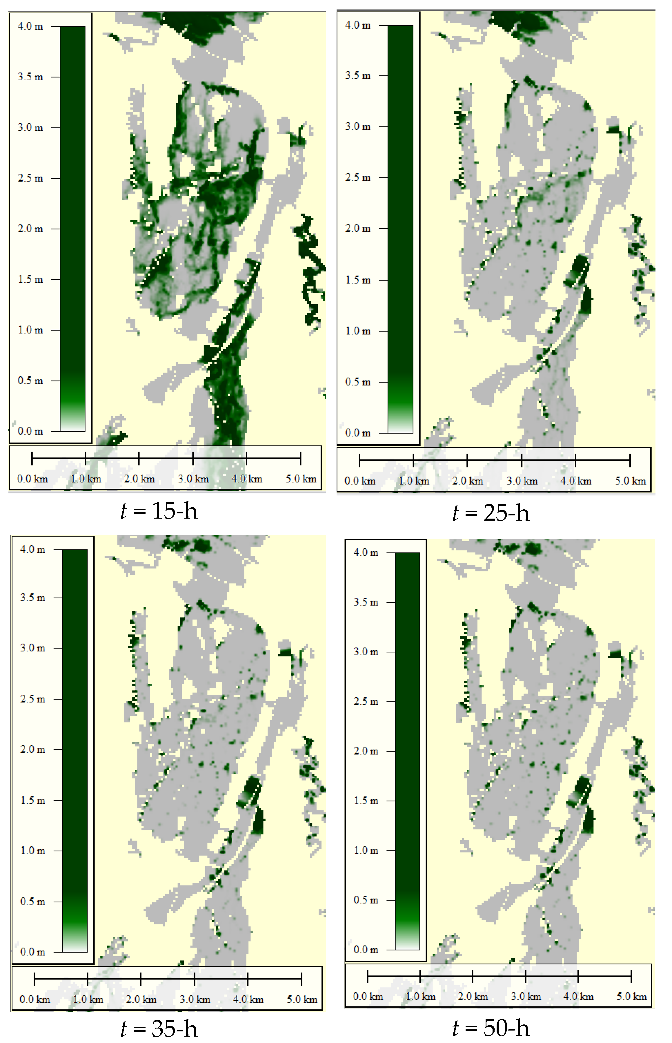
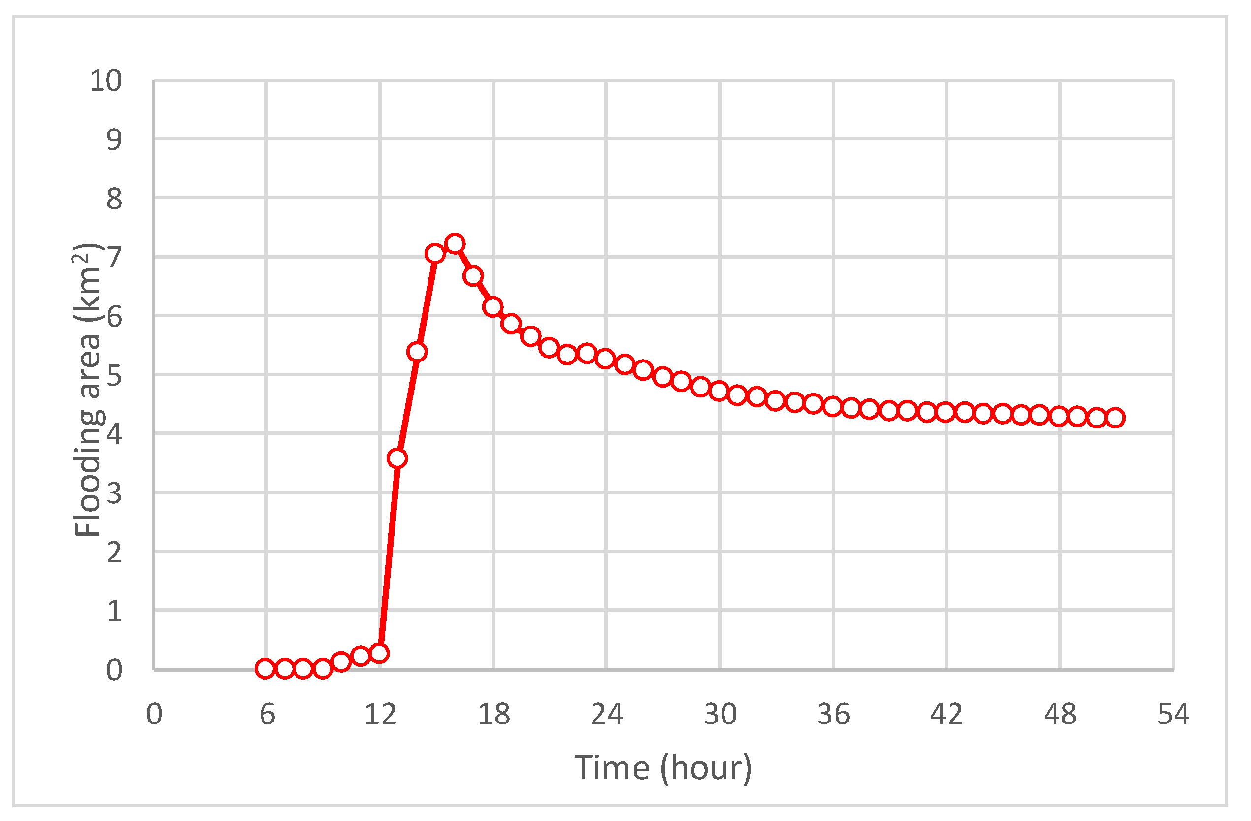
Additionally, Figure 16 shows the maximum and average of the resulting inundation-depth estimates from the SOBEK model, meaning that the average has a slight increase with time from 0 m (t = 8-h) to 0.46 m (t = 32-h); after that, the inundation-depth estimates remain as a constant (about 0.44 m). As for the maximum of the inundation-depth estimates at the VIOT grids, the estimated inundation depth generally increases from 0 m to 4.8 m (t = 15-h), and the maximum approximates a constant (about 0.49 m), indicating that the flood mainly occurs between t = 10-h and t = 15-h; accordingly, the inundation depth sharply rises in 15 h, but slowly drains away until the final time step (t = 51-h). Moreover, by observing the flooding maps composed of the inundation-depth estimate at all VIOT grids regarding the various time steps (see Figure 17), the corresponding inundation area exhibits a similar varying change in time to the maximum inundation-depth estimate in referring to Figure 18, meaning that the flooding area obviously rises with time to the maximum at t = 15-h (approximately 7 km²) and then gradually decreases to 2 km².

As a result, the performance of the proposed SM_EID_VIOT model can be quantified and evaluated in comparison to the results from the SOBEK model, including the inundation-depth estimates of the VIOT grids and flooding areas regarded as the validated data. In detail, the performance for evaluating the difference in the average and maximum of the resulting inundation depths and the flooding area from the SOBEK and SM_EID_VIOT models, respectively, can be described in terms of the root mean square error (RMSE) and coefficient and determination (R²) (i.e., the square of the coefficient of correlation) which are commonly utilized in the evaluation of the ANN-derived models [24,26,27]. Furthermore, to evaluate the accuracy of the proposed SM_EID_VIOT in the quantification of the flooding area composed of the inundation-depth estimates, three types of performance indices, including the precision index, recall-index, and F1-index, are addressed as follows [3]:

$$\mathrm{Precision}=\frac{N_{IG\_EST\_VAL}}{N_{IG\_EST}}$$

(12)

$$\mathrm{Recall}=\frac{N_{IG\_EST\_VAL}}{N_{IG\_VAL}}$$

(13)

$$\mathrm{F}1=2\times \left(\frac{\mathrm{Precision}\times \mathrm{Recall}}{\mathrm{Precision}+\mathrm{Recall}}\right)$$

(14)

where N_{IG_EST} and N_{IG_VAL} serve as the number of the grids regarded as the inundated ones based on the associated nonzero inundation depths estimated by the proposed SM_EID_VIOT model and SOBEK model as the validated data, respectively, and N_{IG_EST_VAL} denotes the number of the inundated grids identified both by the proposed SM_EID_VIOT model and SOBEK model. In referring to Equations (12)–(14), a high precision index means that the grids with the most of the nonzero inundation depths estimated by the proposed SM_EID_VIOT model can be regarded as the inundated ones by the SOBEK model, revealing that the proposed SM_EID_VIOT model can provide the practically inundated grids with high reliability, while a great recall-index value indicates that the inundated grids identified by the proposed SM_EID_VIOT model can also be treated as the inundated ones by the SOBEK model, implying that the proposed SM_EID_VIOT model can capture the practically inundated grids with high likelihood. Eventually, by substituting the precision- and recall-index calculated in Equation (14), the F1-index can be obtained, the high value of which implies that the resulting flooding regions from the proposed SM_EID_VIOT model have excellent agreement with the validated data.

4.4.2. Evaluation of the Inundation-Depth Estimates

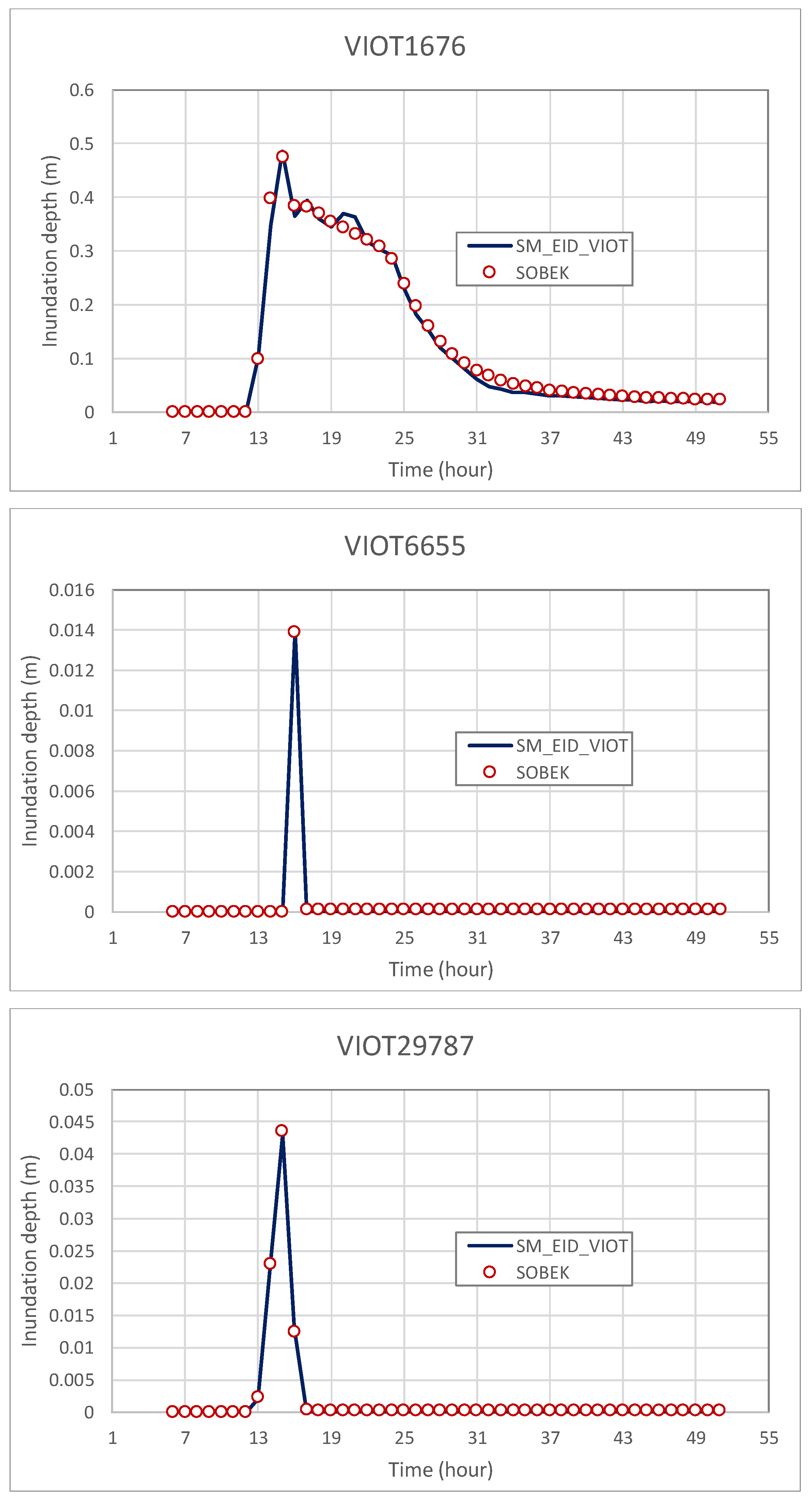
Since the proposed SM_EID_VIOT model aims to estimate the inundation depths at the ungauged locations, named VIOT grids in this study, with the measurements at the experimental roadside IoT sensors, its performance related to the estimations of the inundation depths at the VIOT grids should be evaluated in advance. As mentioned above, the maximum and average estimated inundation depths by the proposed SM_EID_VIOT model can be compared to the validated data, i.e., results from the SOBEK model. From Figure 15, although the validation event mainly begins inundating at t = 13-h, the inundation depths between t = 6-h and t = 51-h are adopted in the model validation to assess the applicability of the proposed SM_EID_VIOT model, which should provide the inundation depths of 0 m as a result of the non-inundation occurred at the IoT sensors. In addition, the three VIOT grids close to the IoT sensors, including the VOT 1676 (TWD97X: 232258.5; TWD97_Y: 2717301), VOT6655 (TWD97X: 234018.6; TWD97_Y: 2718821) and VOT2978 (TWD97X: 232698.5; TWD97_Y: 2718741) are selected in the comparison of the inundation-depth hydrograph. The above relevant results for the model evaluation can be found in Figure 19 and Figure 20 and

Table 6. Performance indices of the resulting inundation-depth estimates from the proposed SM_EID_VIOT model.

Performance Index	Inundation Depth
	Average	Maximum	VIOT1676	VIOT6655	VIOT2978
Root mean square error RMSE (m)	0.103	0.015	0.002	0.000	0.000
Coefficient of determination (R2)	0.891	0.703	0.993	1.000	1.000

.

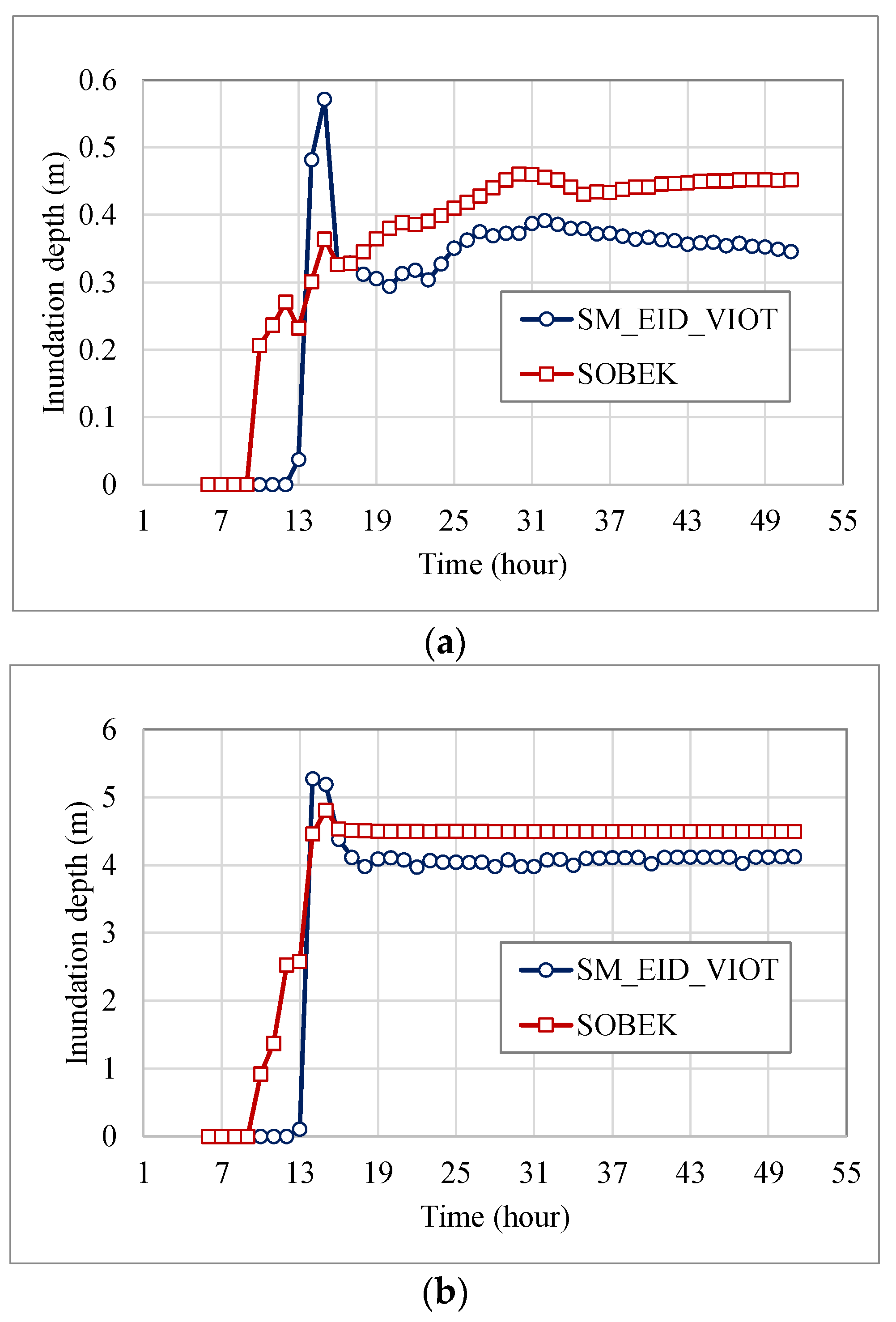
Figure 19 indicates that the average and maximum from the proposed SM_EID_VIOT model are 0 m between t = 6-h and t = 13-h; they steeply rise to the maximum value at t = 13-h and gradually decline with time. A similar conclusion can be found regarding the maximum inundation depth. In detail, as for the average of the inundation-depth estimates at the VIOT girds, the validated data from the SOBEK model significantly exceed the results from the proposed SM_EID_VIOT model, excluding the inundation-depth estimate at t = 14-h and t = 15-h, 0.48 m and 0.57 m, respectively. Among them, the underestimated average and the maximum of the inundation depths via the proposed SM_EID_VIOT model at the time step t less than 13-h are obtained due to the zero inundation depths at the IoT sensors; this reveals that the proposed SM_EID_VIOT model can reasonably produce the inundation depths at the ungauged locations in response to the non-inundation situation at the roadside IoT sensors. Additionally, regarding the results at the time steps t > 13-h, although the average and maximum of the estimated inundation depths via the proposed SM_EID_VIOT model are also less than the validated data, the RMSE values of which are about 0.103 m and 0.015, their varying trend in time have a good match with the validated data as a result of the high coefficient of determination (R²) correlation coefficient of 0.8 (see Table 6). Moreover, in the case of the comparison regarding the inundation-depth hydrograph, as shown in Figure 20, the estimated hydrographs at the specific VIOT grids approach the validated data with a small RMSE value on average, less than 0.002 m. Moreover, the temporal change in the inundation depths estimated by the proposed SM_EID_VIOT model significantly resembles validated data by a high coefficient of determination (R²), over 0.98.

To sum up the above results, the proposed SM_EID_VIOT model can effectively produce the reasonable inundation depths at the ungauged locations based on the observation at the roadside IoT sensors under an acceptable bias and high correlation in time and space. In particular, the accuracy of the inundation depths estimated by the proposed SM_EID_VIOT model can be markedly related to the inverse distance of the corresponding VIOT grids to the roadside IoT sensors.

4.4.3. Assessment of the Flooding Area

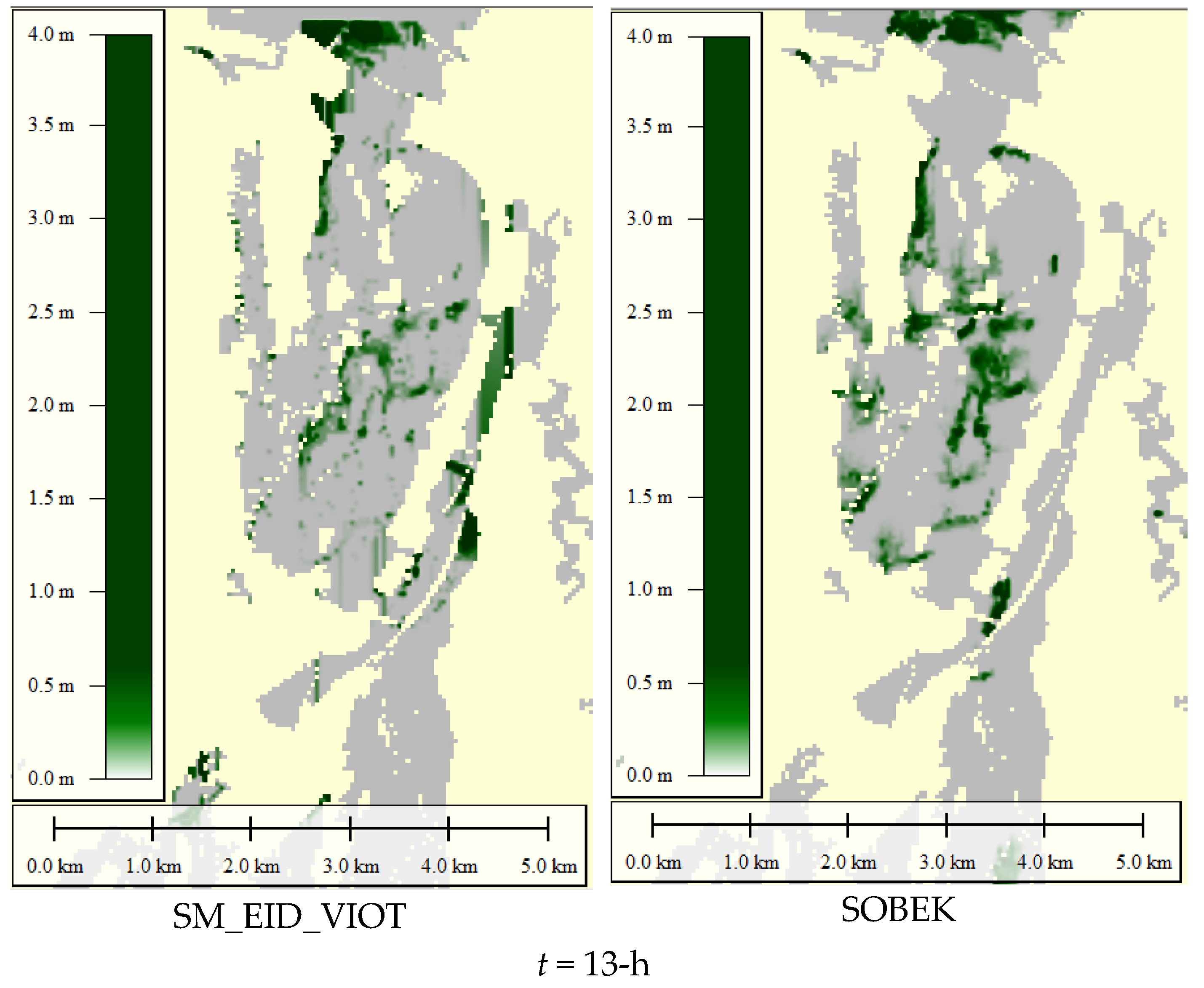
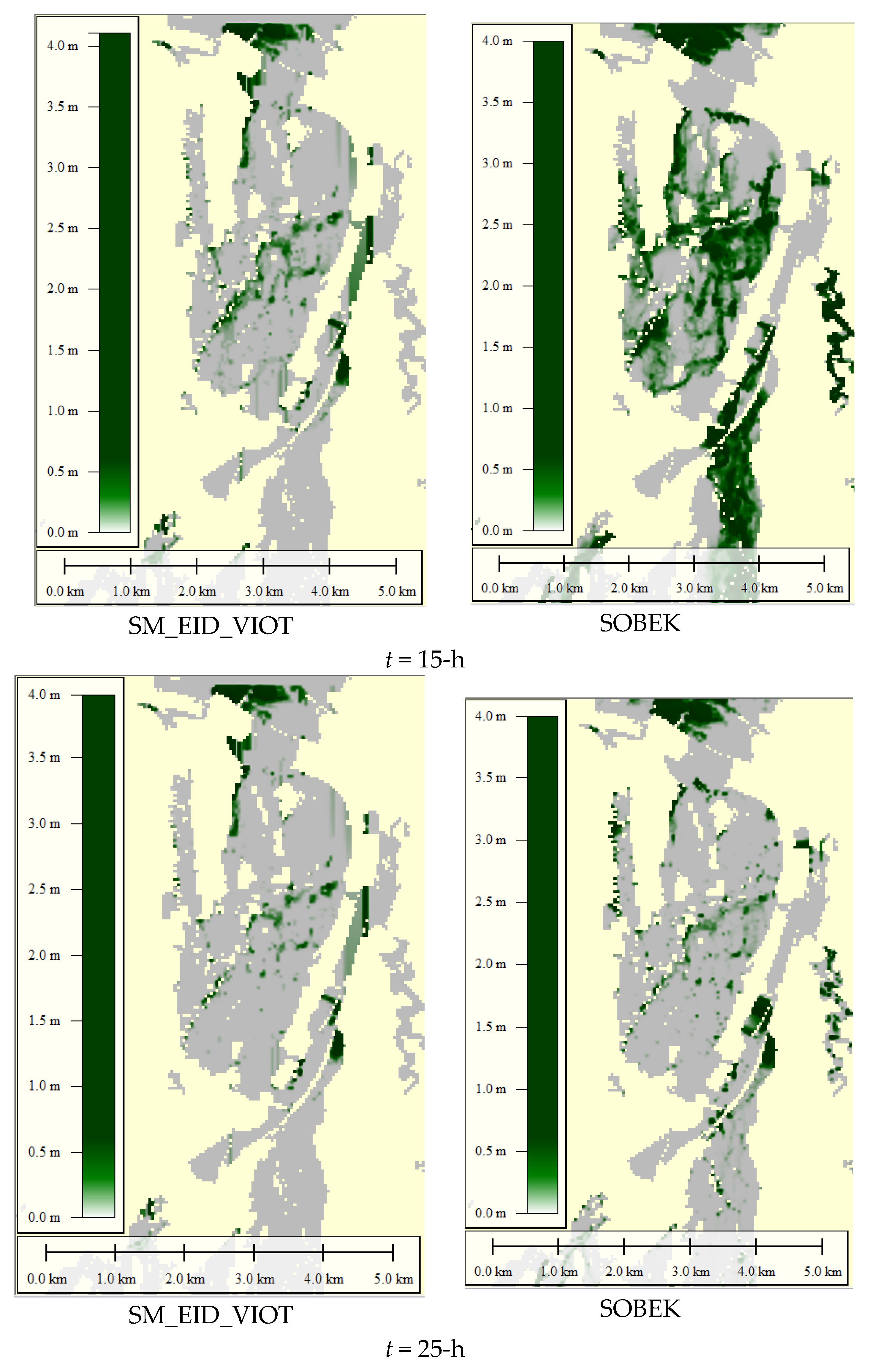
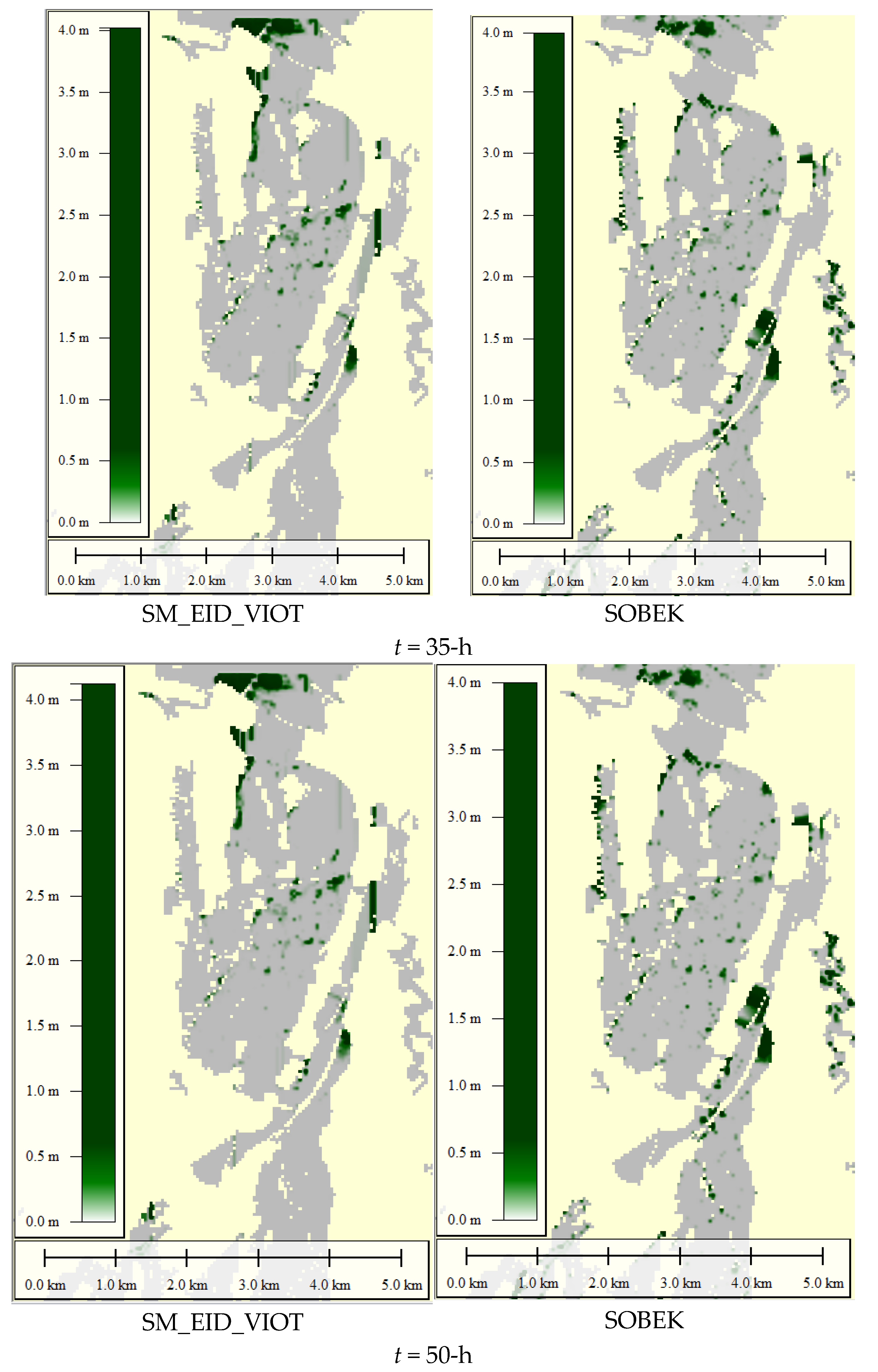
In addition to the evaluation of the gridded inundation depths, the performance for delineating the flooding zones and quantifying the corresponding areas comprised of the estimated inundation depths at the VIOTs grids are supposed to be tested by graphically comparing the validated data at the specific time steps as shown in Figure 21 and Figure 22 and calculating the corresponding performance indices, i.e., the precision-index and recall-index through the Equations (12)–(14) as shown in Figure 21 in which their statistical properties are listed in

Table 7. Statistics of the performance indices of the estimated flooding region.

Performance Index		Precision Index	Recall Index	F1	RMSE (km2)	R2
Statistical properties	Mean	0.669	0.364	0.461	0.161	0.65
	Standard deviation	0.209	0.220	0.208
	Maximum	1.000	1.000	1.000
	Minimum	0.000	0.000	0.000

; additionally, the corresponding root mean square and coefficient of determination (R²) can be found in Table 7.

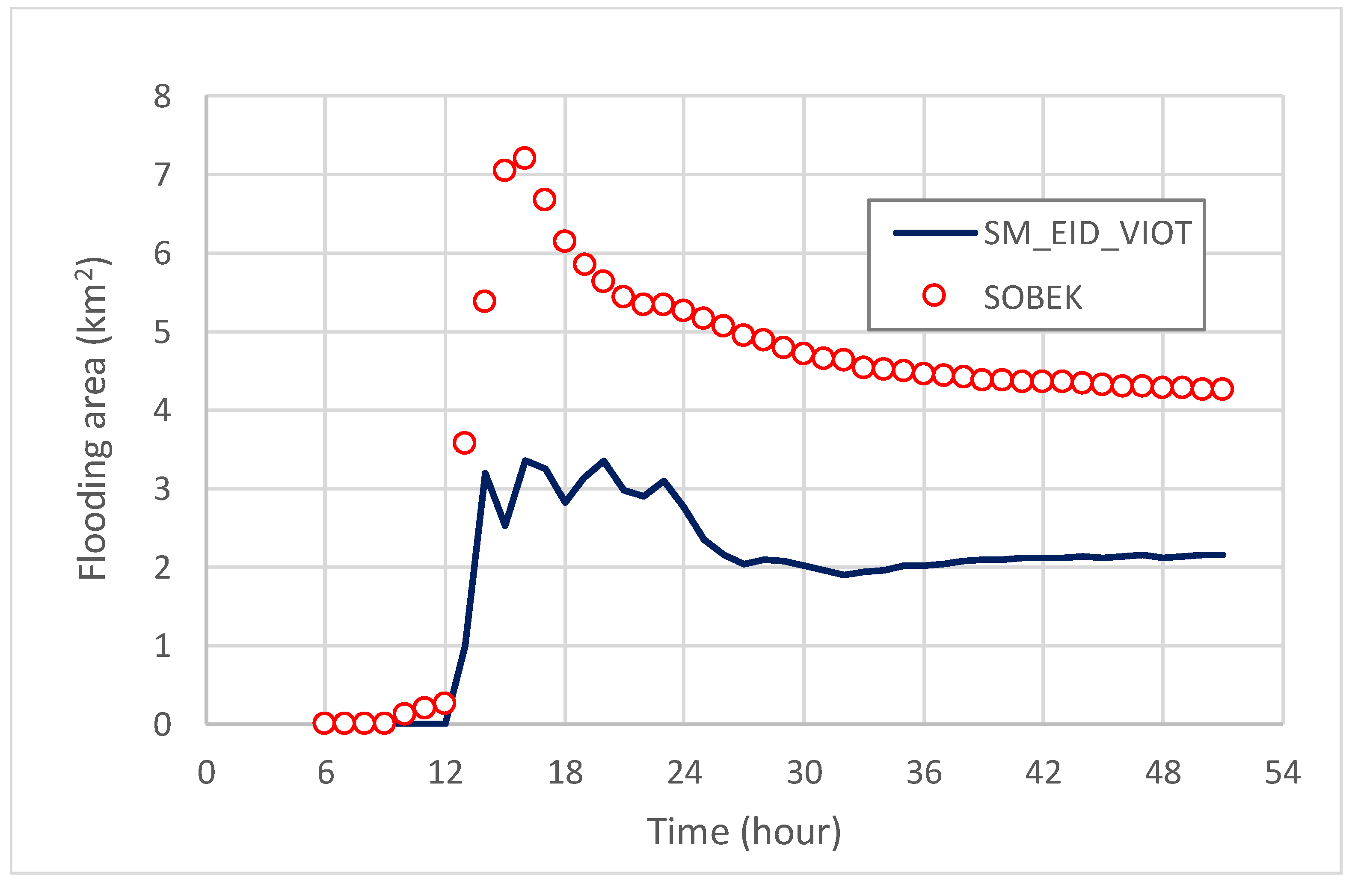
Figure 21 presents the resulting flooding regions from the proposed SM_EID_VIOT model as less than the validated data from the SOBEK model; however, the joint flooding region can be found near the central zone and the three roadside IoT sensors. Additionally, as compared with Figure 22, although the flooding area via the proposed SM_EID_VIOT model increases from t = 6-h to 15-h and then declines with time to a constant in association with the result of the RMSE being 0.161 (km²), the temporal change in the flooding-area estimates is similar to the validated data with a high correlation coefficient of 0.65 (see Table 7).

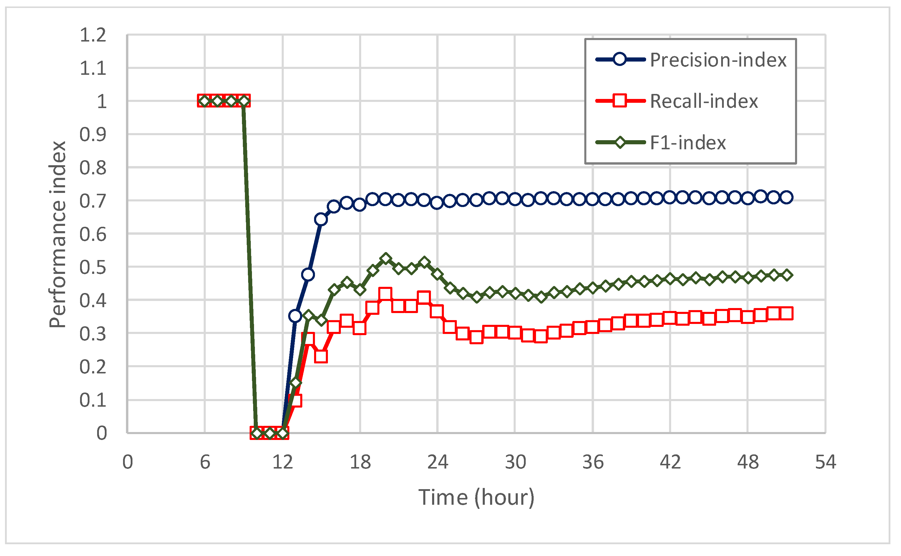
Regarding the performance indices of the resulting flooding region, as shown in Figure 23 and their statistical properties (see Table 7), the performance indices (i.e., the precision and recall index) are equal to 1.0 between t = 6-h and 9-h and 0.0. They are then zero from t = 10-h to t = 12-h, indicating that the performance indices gradually rise with time. Of the performance indices, the precision-index increases from 0.4 to a constant (about 0.7), while the recall index has a similar, varying trend in time, approximately from 0.1 to 0.3. Based on the results from the precision index and recall index, the corresponding F1 index exhibits a similar change with time to the precision and recall indices, excluding those between t = 6-h and t = 12-h in which the magnitudes are 1.0 and 0.0, respectively; the F1 index sharply increases to a constant, approximating 0.5.

In detail, the reason for the high precision and low recall index is that the VIOT grids with the low validated inundation depths obtained by the SOBEK model, probably caused by the light rainfall-induced flood, are excluded as the inundated grids identified by the proposed SM_EID_VIOT model; hence, the amount of the inundation data declines, obtaining the low recall index. Additionally, the proposed SM_EID_VIOT can produce the accurate non-inundation simulation under conditions of IoT sensors with zero inundation-depth observations; nonetheless, the proposed SM_EID_VIOT model could capture the completed flooding zones with somewhat difficulty according to the low recall index (on average 0.4). However, the resulting inundated grids are the accurate flooding locations with a high likelihood based on the high precision index (about 0.7). Eventually, as a result of the F1index, on average, of 0.5, the flooding regions comprising the inundation-depth estimates via the proposed SM_EID_VIOT model can nearly match the validated ones.

In conclusion, it can be proven that the proposed SM_EID_VIOT model can effectively achieve the goal of estimating the inundation depths at the ungauged locations based on the roadside IoT sensors. Additionally, it can delineate the flooding zones to quantify the flood-induced acreage by accounting for the grids of nonzero inundation-depth estimates (named inundated grids) times the grid size. As a result, the proposed SM_EID_VIOT model can provide more reliable and realistic 2D inundation information, including the hydrographs of ungauged inundation depths, the potential flooding regions, and associated area in response to the flood characteristics at the roadside IoT sensors.

5. Conclusions

This study aims to develop the intelligent modeling for estimating the inundation depths at the ungauged locations (i.e., the virtual roadside IoT water-level sensors, VIOT grids) named SM_EID_VIOT model applied in the 2D inundation simulation to obtain the resulting flooding zones and at-site inundation depths. Using the proposed SM_EID_VIOT model, the flooding zones and associated areas could be achieved by combining the inundation-depth estimates at all VIOT grids through the ANN_GA-SA_MTF with the three-layer neural network based on the measurements recorded at the roadside IoT sensors. To carry out the model development and demonstration, the hydrological and geographical data in the Miaoli City of North Taiwan are used in the 1000 simulations of rainfall-induced flood events as the model-training and validating datasets.

According to the results from the model validation, the spatial average and maximum of the estimated inundation depths via the proposed SM_EID_VIOT model have good agreement with those from the validation datasets based on the corresponding low root mean square error (RMSE) of under 0.01 and high coefficient of determination (R²) and over 0.8, respectively, meaning that the inundation-depth estimates at the ungauged grids close to the roadside IoT sensors are significantly correlated with the validated data at the roadside IoT sensors. Nevertheless, the proposed SM_EID_VIOT model could possibly capture the completed flooding zones with some difficulty due to a low recall index of about 0.4, but the resulting inundated grids recognized by the proposed SM_EID_VIOT model are classified as the actual flooding locations with a high precision ratio of approximately 0.7. This reveals that the proposed SM_EID_VIOT model can delineate the flooding zones and quantify the corresponding flooding area in agreement with the validation datasets regarding the spatial variation.

The proposed SM_EID_VIOT can efficiently issue the flooding zones according to the real-time observations at the existing roadside IoT sensors; however, it hardly emulates inundation without the available inundation depths at the IoT sensors during a rainfall-induced flood event. Therefore, selecting the specific ungauged locations as the study spots would be helpful to further enhance the reliability and accuracy of the proposed SM_EID_VIOT model, especially for the delineation of the flooding region by adopting the rainfall factors as the input factors of the ANN-derived model. To simplify the model improvement, the above VIOT grids, where the rainfall factors are treated as the model inputs, can be selected based on the resulting potential flooding-risk maps from the simulations of the rainfall-induced flood events. Eventually, in addition to the observation at the roadside IoT sensor, the relevant flood forecast models which can produce the water-level forecasts at the IoT sensors would be coupled with the proposed SM_EID_VIOT model to provide the gridded inundation-depth forecasts which are advantageous for the flooding early warning and flooding hazard mitigation.

References

- Wu, S.J.; Hsu, C.T.; Chang, C.H. Stochastic modeling of artificial neural networks for real-Time hydrological forecasts based on uncertainties in transfer Functions and ANN weights. Hydrol. Res. 2021, 52, 1490–1525. [Google Scholar] [CrossRef]
- Wu, S.J.; Chang, C.H.; Hsu, C.T. Real-time error correction of two-dimensional flood-inundation simulations during rainstorm events. Stoch. Environ. Res. Risk Assess. 2020, 34, 641–667. [Google Scholar] [CrossRef]
- Kabir, S.; Patidar, S.; Xia, X.; Liang, Q.; Jeffrey Neal, J.; Gareth Pender, G. A deep convolutional neural network model for rapid prediction of fluvial flood inundation. J. Hydrol. 2020, 560, 125841. [Google Scholar] [CrossRef]
- Chen, Y.C.; Chang, T.Y.; Chow, H.Y.; Li, S.L.; Ou, C.Y. Using convolutional neural networks to build a lightweight flood height prediction model with grid-cam for the selection of key grid cells in radar echo maps. Water 2020, 14, 155. [Google Scholar] [CrossRef]
- Ming, X.; Liang, Q.; Xia, X.; Li, D.; Fowler, H.J. Real-time flood forecasting based on a high-performance 2-D hydrodynamic model and numerical weather predictions. Water Resour. Res. 2019, 56, e2019WR025583. [Google Scholar] [CrossRef]
- Ongdas, N.; Akiyanova, F.; Karakulov, Y.; Muratbayeva, A.; Zinabdin, N. Application of HEC-RAS (2D) for Flood Hazard Maps Generation for Yesil (Ishim) River in Kazakhstan. Water 2020, 12, 2672. [Google Scholar] [CrossRef]
- Chang, C.H.; Chung, M.K.; Yang, S.Y.; Chih-Tsung Hsu, C.T.; Wu, S.J. A Case Study for the Application of an Operational Two-Dimensional Real-Time Flooding Forecasting System and Smart Water Level Gauges on Roads in Tainan City, Taiwan. Water 2018, 10, 574. [Google Scholar] [CrossRef] [Green Version]
- Chu, H.; Wu, W.; Wang, Q.J.; Nathan, R.; Wei, J. An ANN-based emulation modelling framework for flood inundation modelling: Application, challenges and future directions. Environ. Model. Softw. 2020, 124, 104587. [Google Scholar] [CrossRef]
- Kwon, S.H.; Kim, J.H. Machine learning and urban drainage systems: State-of –the-art review. Water 2021, 12, 3545. [Google Scholar] [CrossRef]
- Wang, W.C.; Chau, K.W.; Cheng, C.T.; Qiu, L. A comparison of performance of several artificial intelligence methods for forecasting monthly discharge time series. J. Hydrol. 2009, 374, 294–306. [Google Scholar] [CrossRef] [Green Version]
- Ioannou, K.; Myronidis, D.; Lefakis, P.; Stathis, D. The use of artificial neural networks (ANNs) for the forecast of precipitation levels of lake Doirani (N. Greece). Fresenius Environ. Bull. 2010, 19, 1921–1927. [Google Scholar]
- Chang, L.C.; Shen, H.Y.; Chang, F.J. Regional flood inundation nowcast using hybrid SOM and dynamic neural networks. J. Hydrol. 2014, 519, 476–489. [Google Scholar] [CrossRef]
- Huashi, A.O.; Abdirahman, A.A.; Elmi, M.A.; Hashi, S.Z.M.; Rodriguez, O.E.R. A real-time flood detection system based on machine learning algorithms with emphasis on deep learning. Int. J. Eng. Trends Technol. 2021, 69, 219–256. [Google Scholar]
- Wu, S.J.; Hsu, C.T.; Chang, C.H. Stochastic Modeling for Estimating Real-Time Inundation Depths at Roadside IoT Sensors Using the ANN-Derived Model. Water 2021, 12, 3128. [Google Scholar] [CrossRef]
- Sit, M.; Demiray, B.Z.; Xiang, Z.; Ewing, G.J.; Sermet, Y.; Demir, I. A comprehensive review of deep learning applications in hydrology and water resources. Water Sci. Technol. 2020, 82, 2635–2670. [Google Scholar] [CrossRef]
- Khashei, M.; Bijiai, M. An artificial neural network (p, d, q) model for timeseries forecasting. Expert Syst. Appl. 2010, 37, 479–489. [Google Scholar] [CrossRef]
- Mustafa, M.R.; Rezaur, R.B.; Rahardjo, H.; Isa, M.H.; Arif, A. Artificial Neural Network Modeling for Spatial and Temporal Variations of Pore-Water Pressure Responses to Rainfall. Adv. Meteorol. 2015, 2015, 273730. [Google Scholar] [CrossRef] [Green Version]
- Chang, L.C.; Amin, M.Z.M.; Yang, S.N.; Chang, F.J. Building ANN-Based Regional Multi-Step-Ahead Flood Inundation Forecast Models. Water 2018, 10, 1283. [Google Scholar] [CrossRef] [Green Version]
- Tu, J.V. Advantages and disadvantages of using artificial neural networks versus logistic Regression for predicting medical outcomes. J. Clin. Epidemiol. 1996, 49, 1225–1231. [Google Scholar] [CrossRef]
- Najafzadeh, M.; Zahiri, A. Neuro-Fuzzy GMDH-Based Evolutionary Algorithms to Predict Flow Discharge in Straight Compound Channels. J. Hydrol. Eng. 2015, 20, 04015035. [Google Scholar] [CrossRef]
- Delasalles, E.; Ziat, A.; Denoyer, L.; Gallinari, P. Spatio-temporal neural networks for space-time data modeling and relation discovery. Knowl. Inf. Syst. 2019, 61, 1241–1267. [Google Scholar] [CrossRef]
- Amiri, M.A.; Zmerian, Y.; Mesgari, M.S. Spatial and temporal monthly precipitation forecasting using wavelet transform and neural network, Qara-Qum catchment, Iran. Arab. J. Geosci. 2016, 9, 421–438. [Google Scholar] [CrossRef]
- Wu, S.J.; Hsu, C.T.; Chang, C.H. Stochastic modeling of gridded short-term rainstorms. Hydrol. Res. 2021, 52, 876–904. [Google Scholar] [CrossRef]
- Delft Hydraulics. SOBEK Software User’s Manual; WL|Delft Hydraulics: Delft, The Netherlands, 2013; Available online: https://content.oss.deltares.nl/delft3d/manuals/SOBEK_User_Manual.pdf (accessed on 6 June 2022).
- Chang, C.H.; Yang, J.C.; Tung, Y.K. Incorporate marginal distributions in point estimate methods for uncertainty analysis. J. Hydraul. Eng. 1997, 123, 244–251. [Google Scholar] [CrossRef] [Green Version]
- Nataf, A. Determination des distributions don’t les marges sontdonnees. Comptes Rendus L’académie Sci. 1962, 225, 42–43. [Google Scholar]
- Wu, S.J.; Lien, H.C.; Chang, C.H. Calibration of a conceptual Rainfall-Runoff Model using a Genetic Algorithm Integrated with Runoff Estimation Sensitivity to Parameters. J. Hydroinform. 2011, 14, 497–511. [Google Scholar] [CrossRef]
- Wu, S.J.; Lien, H.C.; Chang, C.H.; Shen, J.C. Real-Time Correction of Water Stage Forecast during Rainstorm Events Using Combination of Forecast Errors. Stoch. Environ. Res. Risk Assess. 2012, 26, 519–531. [Google Scholar] [CrossRef]
- Wu, S.J.; Chen, P.H.; Yang, J.C. Application of Weighted Semivariogram Model (WSVM) based on fitness to experimental semivariogram on estimation of rainfall amount. Hydrol. Earth Syst. Sci. Discuss. 2011, 8, 4229–4259. [Google Scholar]
Figure 1.
The graphic framework of the development and application regarding the proposed SM_EID_VIOT model.
Figure 2.
Graphical process of extracting the gridded rainfall characteristics from observed photographs of rainstorm events [22].
Figure 3.
The brief graphical framework for estimating the inundation depths at the VIOT spots via the ANN_GA-SA_MTF model within the SM_EID_VIOT model.
Figure 4.
The framework for the development and application of the proposed SM_EDI_VIOT model.
Figure 5.
Location of Miaoli County (note: blue circles are the radar-precipitation grid, and red points are the roadside IoT sensors).
Figure 6.
The DEM of Miaoli County.
Figure 7.
Summary of the gridded rainfall characteristics from 50 historical rainstorms in Miaoli County.
Figure 8.
Spatial distributions of gridded rainfall depths at specific times in Miaoli County.
Figure 9.
2D SOBEK model for Miaoli County.
Figure 10.
Graphical illustration of the flooding area within Miaoli County drawn based on the maximum of the resulting inundation depths.
Figure 11.
Potential inundation zones within Miaoli County.
Figure 12.
Locations of VIOT grid and IoT sensors within Miaoli City.
Figure 13.
Summary of the estimation of the number of hidden neurons via various methods.
Figure 14.
Summary of the transfer function weights for calculating the weighted average of inundation-depth estimates.
Figure 15.
The SOBEK model simulated inundation-depth hydrographs at the IoT sensors for the 921st simulation case as the validated data.
Figure 16.
Maximum and average of the simulated inundation depths at the VIOT grids in the SOBEK model for the 921st simulation case.
Figure 17.
Resulting flood map from the SOBEK model in study area Miaoli City.
Figure 18.
Flooding-area hydrograph estimated by the SOBEK model in study area Miaoli City.
Figure 19.
Comparison of the average and maximum of the inundation depths at the VIOT grids by the proposed SM_EID_VIOT model with the validated data. (a) Average inundation depth. (b) Maximum inundation depth.
Figure 20.
Comparison of the resulting inundation-depth hydrograph at the specific VIOT grids from the proposed SM_EID_VIOT model with the validated data.
Figure 21.
Comparison of the estimated flooding regions via the proposed SM_EID_VIOT model with results from the SOBEK model at the specific time steps.
Figure 22.
Comparison of flooding-area hydrograph quantified estimated via the proposed SM_EID_VIOT model with the results from the SOBEK as validated data.
Figure 23.
Summary of the performance indices of the estimated flooding region by the proposed SM_EID_VIOT model.