Hydrological Retrospective and Historical Drought Analysis in a Brazilian Savanna Basin

Abstract

Analyzing historical droughts is essential to improve the assessment of future hydrological risks and to understand the effects of climate variability on streamflow. However, prolonged and consistent hydrological time series are scarce in the Brazilian savanna region. This study aimed to analyze the performance of climate reanalysis products in precipitation estimation, hydrological modeling, and historical drought analysis in a Brazilian savanna basin. For this purpose, precipitation data from the twentieth-century atmospheric model ensemble (ERA-20CM) and the land component of the fifth generation of European ReAnalysis (ERA5-Land) with bias correction were used. The weather variables were obtained from the Climatic Research Unit (CRU) and the hydrological modeling was performed using the Soil and Water Assessment Tool (SWAT). The Standardized Streamflow Index (SSI) was used to calculate hydrological drought in the basin. Overall, ERA5-Land performed satisfactorily in precipitation estimation, mainly on the monthly time scale, hydrological modeling, and drought prediction. Since ERA-20CM showed unsatisfactory values for the performance statistics in all analyses, the hydrologic drought (1950 to 2018) was performed with ERA5-Land. The results showed both an increase in the number of dry months and a decrease in wet months in recent decades.

1. Introduction

Understanding the hydrological condition and its spatial and temporal behavior is important in many disciplines, such as water resources and natural hazards [1]. Long and consistent hydrometeorological data are needed to better comprehend the hydrological cycle components in watersheds. However, these data are scarce in many Brazilian regions, presenting gaps and a low network density of observed data, which limit their use in hydrological studies [2,3,4].

To overcome the lack of long-term hydrometeorological data, recent studies have sought to produce climate reanalysis, i.e., a consistent reprocessing of archived weather observations using modern forecasting systems [5]. Some groups have produced global climate reanalysis data at a fine spatial and temporal resolution, such as the European Centre for Medium-Range Weather Forecasts (ECMWF), which has different products that have reconstructed several climate variables, including many that are not directly observed, since the early twentieth century.

Climate reanalysis provides continuous estimates of weather variables, including precipitation, for any terrestrial location worldwide, extending over several decades [6]. Contrasting with ground measured data, reanalysis is uniform in time and space and provides spanned weather elements [7]. Given this, climate reanalysis has been considered a surrogate for local observations since the 1990s [8].

The climate reanalysis has presented satisfactory results [9,10]. However, since these products use observed data for assimilation, atmospheric forcing, and boundary conditions (e.g., [11,12,13]), there is a greater uncertainty for the older years due to the lower availability of observational sources in relation to recent decades. In addition, the quality of the climate reanalysis data varies by region because the same product may present different performances according to the study area [8], and it is influenced by a non-uniform monitoring network. Therefore, more studies are needed to evaluate its applicability in different climate regions and its reliability for older years.

When associated with hydrological models, the climate reanalysis allows the simulation of long and consistent hydrometeorological variables, such as streamflow series. This process is known as Hydrological Retrospective (HR) [14]. According to Auerbach et al. [6], HR is required for applications focused on seasonal and interannual variability to assess water supply risk and ecological studies. Some researchers have adopted this methodology and achieved satisfactory results [1,14,15,16]. In Brazil, Correa et al. [14,17] addressed HR in the Amazon basin; however, there are no studies involving HR in Brazilian savanna basins, an ecologically relevant [18,19] and important biome for freshwater distribution in South America [20].

HR can also be important for assessment of historical drought events, which is essential to improve our understanding of the hydrological risks and the effects of climate variability [14]. Managing the impacts of the deficit on the hydrological system is currently one of the main concerns of water resources managers across the globe [21,22], since this deficit can affect the ecological system [23,24], several economic sectors [23], and the urban population [25]. Although the number of hydrological drought studies in the Brazilian savanna has increased in recent years (e.g., [26,27,28]), there is still limited research related to the occurrence of drought events for longer periods in the past, mainly due to limitations involving the observed data. Therefore, HR is expected to improve the understanding of past extreme events, contributing to better management of the impacts caused by droughts.

In this context, this study aimed to (i) validate different precipitation products of climate reanalysis in a Brazilian savanna basin; (ii) analyze the performance of these products in hydrological modeling; (iii) test the simulated streamflow based on reanalysis products in predicting the occurrence of hydrological droughts; and (iv) perform HR and historical drought analysis in the basin.

2. Materials and Methods

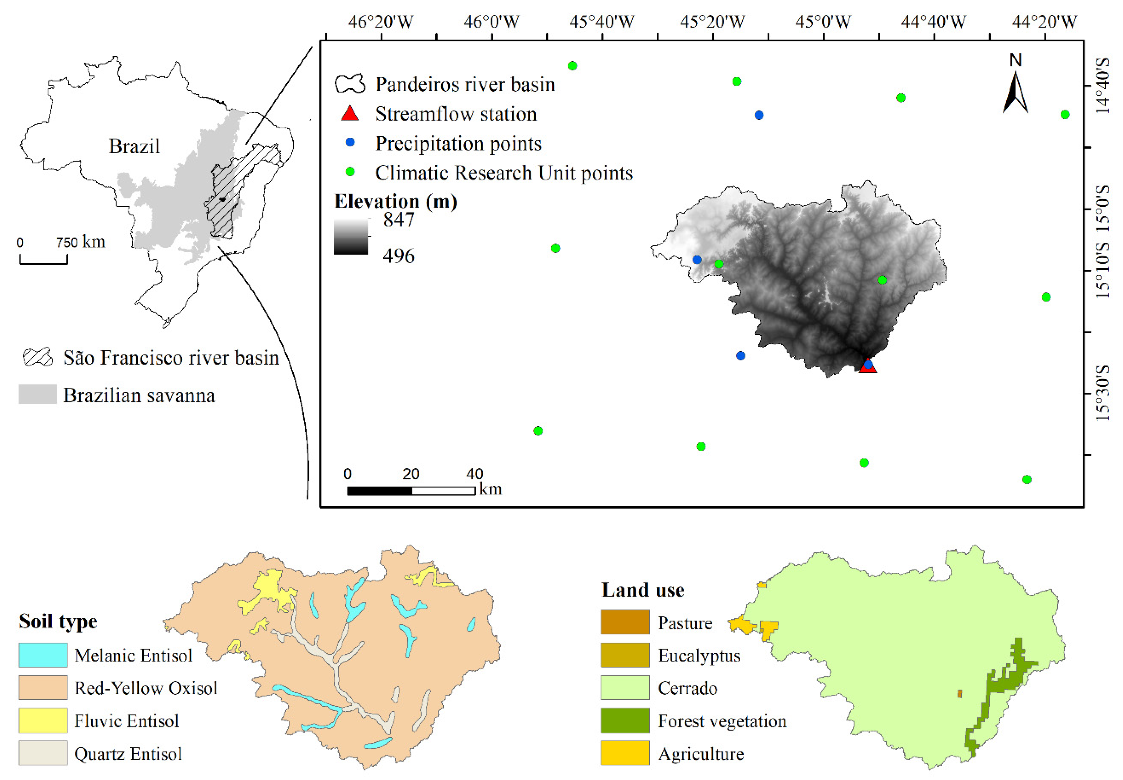
2.1. Study Area

The Pandeiros River basin (PRB), delimited from the “Usina do Pandeiros Montante” streamflow station, has an area of 3220 km² and is completely inserted in the Brazilian savanna [29]. Its altitude varies from 496 to 897 m, with an average of 677 m, and an average slope of 5.9%. Figure 1 presents the PRB location, the streamflow station, and the Digital Elevation Model (DEM) ALOS (Advanced Land Observing Satellite) PALSAR (Phased Array L-band Synthetic Aperture Radar), with a spatial resolution of 12.5 m.

PRB is strategically used for the reproduction and development of the ichthyofauna of the São Francisco River midstream [30]. To protect the growth and reproduction of native fish species, the Pandeiros River Environmental Protection Area was created in 1995 through State Law no. 11,901, the largest unit for sustainable use in Minas Gerais State [31].

The Köppen climate type for PRB is tropical, with predominant precipitation in summer and dry winter (Aw). According to the Thornthwaite climate classification, the climate is defined as dry sub-humid (C1) [32]. The annual temperature varies from 17.9 °C to 31.6 °C, with an average of 23.8 °C.

The average annual precipitation in the PRB is 1085 mm, of which 92% occurs during the rainy period (October to March), and evapotranspiration corresponds to 81.4% of rainfall [33]. The precipitation in the Brazilian savanna is significantly influenced by the South Atlantic Convergence Zone (SACZ), which is characterized by the coupling of the convergent winds and moisture to transient vortices from higher latitudes and remains quasi-stationary for several days, mainly in the austral summer (December to February) [34,35]. In addition, other climatic phenomena, such as the El Niño-Southern Oscillation (ENSO), can influence precipitation in the basin [33].

2.2. SWAT Model

The Soil and Water Assessment Tool (SWAT) [36] is a physically based hydrological model developed to simulate and predict the impacts of management on water, sediment, and agricultural chemicals in basins over long periods [37]. In this model, the basin is divided into multiple sub-basins, subdivided into Hydrological Response Units (HRUs), which are territorial units with similar hydrological behavior [38]. SWAT is based on the water balance in each of the HRUs, according to Equation (1) [39].

$${\mathrm{SW}}_{\mathrm{t}}{=\mathrm{SW}}_0+{\displaystyle \sum }_{\mathrm{i}=1}^{\mathrm{t}}{(\mathrm{R}}_{\mathrm{day}}-{\mathrm{Q}}_{\mathrm{surf}}-{ \mathrm{E}}_{\mathrm{a}}-{\mathrm{w}}_{\mathrm{seep}}-{\mathrm{Q}}_{\mathrm{gw}})$$

(1)

where SW_t is the final soil water content (mm); SW₀ is the initial soil water content on the day i (mm); t is the time (days); R_day is the amount of precipitation on the day i (mm); Q_surf is the amount of surface runoff on the day i (mm); E_a is the amount of evapotranspiration on the day i (mm H2O); w_seep is the amount of water entering the vadose zone from the soil profile on the day i (mm); Q_gw is the amount of return flow on the day i (mm).

In this study, the Curve Number (CN) method [39] was used to estimate the surface runoff from HRUs, and the Penman–Monteith equation [40,41] to estimate the evapotranspiration in the basin. The variable storage routing method [42] was adopted for routing the water through the channel network.

2.3. SWAT Model Input Data

Daily streamflow was obtained from the Brazilian National Water Agency (ANA) to calibrate and validate SWAT from August 1973 to December 2018. The weather variables (mean, minimum, and maximum temperatures, and vapor pressure) were obtained from the Climatic Research Unit (CRU) Time Series (TS) version 4.04 from 1901 to 2018 at a spatial resolution of 0.5° and monthly time scale [43].

As the wind speed is not available in CRU TS v. 4.04 and has low monthly variability [44], it was obtained from the monthly climatological normal for the period 1961–1990 from CRU CL version 2.0 [45], at the same points as CRU TS v. 4.04, and replicated for the entire period (1901–2018). This product provides wind speed data at 10 m in height, which was converted to 1.7 m [46]. Solar radiation (derived from Hargreaves methodology) and relative humidity were estimated according to the methodology of Allen et al. [44]. The location of hydrometeorological variables and maps of soil type and land use are in Figure 1.

The soil type [47] and land use maps [48] at a scale of 1:650,000 and 1:1,000,000, respectively, were used to generate the HRUs. The DEM (Figure 1) was used to generate the slope map, which was divided into four classes: 0–3%, 3–5%, 5–8%, and >8%. The Red-Yellow Oxisol (LVA) is the predominant soil unit in the PRB (88.3% of the basin’s area), followed by the Fluvic Entisol (RQ, 4.1%), Quartz Entisol (RY, 4.0%), and Melanic Entisol (GM, 3.7%). Cerrado is the predominant land use (CERR, 96.3%), followed by agriculture (AGRL, 2.0%), forest vegetation (FRST, 1.7%), and pasture (PAST, 0.1%).

2.4. Reanalysis Data

2.4.1. ERA-20CM

The twentieth-century atmospheric model ensemble (ERA-20CM) is an ensemble of ten atmospheric model integrations that provide data from 1900 to 2010. Its resolution is T159 (approximately 125 km in grid-point space) in the spectral horizon, using 91 levels in the vertical from the surface up to 1 Pa (approximately 80 km altitude), and a time step of one hour [11,49].

According to Hersbach et al. [11], ERA-20CM is a variation in the atmosphere and ocean-wave forecast model components of Cy38r1, and daily sea surface temperature (SST) and sea ice cover are prescribed by an ensemble of ten realizations (HadISST2.1). These realizations are a biased reflection of the estimates and uncertainties in the observed sources. The forcing terms in the model radiation scheme follow Coupled Model Intercomparison Project Phase 5 recommendations, which incorporate both long-term climate evolution and the periodic occurrence events, such as the El Niño-Southern Oscillations and volcanic eruptions.

In this study, we used the ten ERA-20CM ensemble members (Ens0 to Ens9) with precipitation data every 3 h, accumulated for a daily scale, and a 0.125° × 0.125° grid from January 1900 to December 2010 [11,50]. The values of the ten ERA-20CM ensemble members were averaged (AE) for further analysis.

2.4.2. ERA5-Land

The land component of the fifth generation of European ReAnalysis (ERA5-Land) is a reanalysis dataset that produces precipitation and 52 other variables describing the water and energy cycle globally over land, with a temporal resolution of 1 h and spatial resolution of 9 km. This dataset is available from January 1950 to the present (with up to a 3-month lag) [12,51,52].

The land surface model used in the ERA5-Land production is the Carbon Hydrology-Tiled ECMWF Scheme for Surface Exchanges over Land (CHTESSEL) from the model cycle Cy45r1. The ERA5-Land does not assimilate observations directly; however, atmospheric observations (air temperature, specific humidity, wind speed, and surface pressure) are added as atmospheric forcing and corrected using a daily lapse rate correction derived from ERA5 [12]. According to Muñoz-Sabater [51], these forcings are essential so that the model estimates do not deviate from the real pattern.

This study uses the accumulated hourly precipitation data, which was converted to a daily time scale from January 1950 to December 2018 [51,52].

2.5. Bias Correction

Several methodologies have been developed to remove the bias of the precipitation outputs from climatic models, among which the linear scaling (LSC) [53] stands out due to its simplicity and efficiency [17]. This method is based on the difference between observed precipitation (OP) and estimated precipitation, corrected with a factor based on the long-term monthly average ratio [54], according to Equation (2).

$${\mathrm{P}}_{\mathrm{rean}}^{\ast }{=\mathrm{P}}_{\mathrm{rean}}\times \left[\frac{{\mathsf{\mu }}_{\mathrm{m}}\left({\mathrm{P}}_{\mathrm{obs}}\right)}{{\mathsf{\mu }}_{\mathrm{m}}\left({ \mathrm{P}}_{\mathrm{rean},\mathrm{obs}}\right)}\right]$$

(2)

where ${\mathrm{P}}_{\mathrm{rean}}^{\ast }$ is the final value of precipitation with bias correction; P_rean is the precipitation without bias correction; P_obs is the observed precipitation; P_rean,obs is the precipitation without bias correction for the period when observed data are available; µ_m is the average parameter of the normal distribution for month m.

This study applied the bias correction to the ten ERA-20CM ensemble members, the AE, and the ERA5-Land.

2.6. Calibration, Validation, and Uncertainty Analysis

The SWAT-CUP software package version 5.2.1 with the SUFI-2 algorithm was used for calibration, validation, and uncertainty analysis. According to Abbaspour et al. [55], this algorithm seeks all uncertainties (parameter, conceptual model, input, etc.) on the parameters and tries to envelop most of the observations within the 95% prediction uncertainty (95PPU) of the model. The 95PPU is calculated at the 2.5% and 97.5% levels of the cumulative distribution of an output variable using Latin hypercube sampling.

In this study, the calibration (2004–2011) was carried out with OP of four rain gauge stations from ANA (station codes 1545006, 1445000, 1545005, and 1544032) and CRU climate data, with the warm-up period from June 2000 to December 2003. The initial parameters were selected based on previous studies in the basin [56]. It used two iterations of 600 simulations each and Nash–Sutcliffe efficiency (NSE) as the objective function. The best set parameters and the final range obtained in the calibration were replicated in the validation phase with OP and CRU setup from January 2012 to December 2018. Afterward, the validation of the hydrological simulation with the ten ERA-20CM ensemble members, AE, and ERA5-Land with bias correction and CRU climate data was conducted with the best parameters obtained in the calibration phase from August 1973 to December 2010.

The uncertainty during the calibration and validation phases with OP and CRU data was quantified using two statistics: p-factor, which relates to the percentage of observed data enveloped by the modeling result, the 95PPU; and r-factor, which is associated with the thickness of the 95PPU envelop [57]. Abbaspour et al. [55] highlighted that there should be a balance between these two indices; however, p-factor >0.7 and r-factor <1.5 for discharge are recommended.

2.7. Performance of Precipitation and Hydrological Modeling

To analyze the quality of estimated precipitation data and identify the reanalysis product that most adequately represents the past climatic conditions, the ten ERA-20CM ensemble members, AE, and ERA5-Land were compared with the OP on daily and monthly time scales through the point-to-pixel approach, using the most extended as possible same period between the reanalysis and OP products. This methodology compares the rain gauge values with the corresponding pixel value of reanalysis products [58]. For this purpose, the Pearson correlation coefficient (r), Root Mean Square Error (RMSE), and Kling–Gupta efficiency (KGE) were used (

Table 1. Statistical metrics used to evaluate the performance of precipitation and hydrological modeling with reanalysis products for the PRB.

Statistical Metrics	Equation	Ideal Value	Unit
Pearson correlation coefficient	$\mathrm{r}=\frac{{{\displaystyle \sum }}_{\mathrm{i}=1}^{\mathrm{N}}\left({\mathrm{O}}_{\mathrm{i}}-{\mathrm{O}}_{\mathrm{m}}\right){\times (\mathrm{E}}_{\mathrm{i}}-{\mathrm{E}}_{\mathrm{m}})}{\sqrt{{{\displaystyle \sum }}_{\mathrm{i}=1}^{\mathrm{N}}{\left({\mathrm{O}}_{\mathrm{i}}-{\mathrm{O}}_{\mathrm{m}}\right)}^2\times {{\displaystyle \sum }}_{\mathrm{i}=1}^{\mathrm{N}}{{(\mathrm{E}}_{\mathrm{i}}-{\mathrm{E}}_{\mathrm{m}})}^2}}$	1	-
Root Mean Square Error	$\mathrm{RMSE}=\sqrt{\frac{{{\displaystyle \sum }}_{\mathrm{i}=1}^{\mathrm{N}}{\left({\mathrm{E}}_{\mathrm{i}}-{\mathrm{O}}_{\mathrm{i}}\right)}^2}{\mathrm{N}}}$	0	mm
Kling–Gupta efficiency	$\mathrm{KGE}=1-\sqrt{{\left(\mathrm{r}-1\right)}^2+{\left(\mathsf{\beta }-1\right)}^2+{\left(\mathsf{\gamma }-1\right)}^2}$ $\mathsf{\beta }=\frac{{\mathrm{E}}_{\mathrm{m}}}{{\mathrm{O}}_{\mathrm{m}}}$ $\mathsf{\gamma }=\frac{{\mathsf{\sigma }}_{\mathrm{E}}{/\mathrm{E}}_{\mathrm{m}}}{{\mathsf{\sigma }}_{\mathrm{O}}{/\mathrm{O}}_{\mathrm{m}}}$	1	-
Percent bias	$\mathrm{PBIAS}=\left[\frac{{{\displaystyle \sum }}_{\mathrm{i}=1}^{\mathrm{N}}{(\mathrm{O}}_{\mathrm{i}}-{\mathrm{E}}_{\mathrm{i}})}{{{\displaystyle \sum }}_{\mathrm{i}=1}^{\mathrm{N}}{\mathrm{O}}_{\mathrm{i}}}\right]\times 100$	0	%
Nash–Sutcliffe efficiency	$\mathrm{NSE}=1-\left[\frac{{{\displaystyle \sum }}_{\mathrm{i}=1}^{\mathrm{N}}{{(\mathrm{O}}_{\mathrm{i}}-{\mathrm{E}}_{\mathrm{i}})}^2}{{{\displaystyle \sum }}_{\mathrm{i}=1}^{\mathrm{N}}{{(\mathrm{O}}_{\mathrm{i}}-{\mathrm{O}}_{\mathrm{m}})}^2}\right]$	1	-
Logarithmic Nash–Sutcliffe efficiency	$\mathrm{LNSE}=1-\left\{\frac{{{\displaystyle \sum }}_{\mathrm{i}=1}^{\mathrm{N}}{\left[\log \left({\mathrm{O}}_{\mathrm{i}}\right)-\log \left({\mathrm{E}}_{\mathrm{i}}\right)\right]}^2}{{{\displaystyle \sum }}_{\mathrm{i}=1}^{\mathrm{N}}{\left[\log \left({\mathrm{O}}_{\mathrm{i}}\right)-\log \left({\mathrm{O}}_{\mathrm{m}}\right)\right]}^2}\right\}$	1	-

Note(s): E and O are the estimated and observed variables, respectively; E_m and O_m are the averages of the estimated and observed variables, respectively; σ_E and σ_O are the standard deviations of the estimated and observed variables, respectively; i is the time sequence of observed and simulated pairs; N is the number of observed and simulated pairs; β is a bias term; and γ measures the streamflow variability error.

).

KGE, percent bias (PBIAS), NSE, and its logarithmic version (LNSE) (Table 1) were used in this study to analyze the performance of best fit in the hydrological modeling. Moriasi et al. [59] developed an overall performance rating for NSE and PBIAS to evaluate the model during the calibration and validation in a monthly time step: “very good” (NSE > 0.75; PBIAS < ±10); “good” (0.65 < NSE ≤ 0.75; ±10 ≤ PBIAS < ±15); “satisfactory” (0.50 < NSE ≤ 0.65; ±15 ≤ PBIAS < ±25); and “unsatisfactory” (NSE ≤ 0.50; PBIAS ≥ ±25). Because of the similarities, the same classification of NSE was used for the LNSE. KGE values above 0.6 are generally considered good [10].

2.8. Hydrological Drought Analysis

The Standardized Streamflow Index (SSI) is a hydrological drought index, helpful in making comparisons over a wide variety of river regimes and flow characteristics [60]. In this study, the SSI was calculated to validate the hydrological drought with simulated streamflow (from 1973 to 2010) and then calculate the historical drought with the simulation that provided the best streamflow estimates.

To calculate the SSI, the hydrological year mean annual observed and simulated streamflow was considered (October to September). In this historical series, the Gamma probability density function (PDF) was fitted. Then, the inverse normal distribution was used to obtain the respective “z” value for each non-exceeded probability prior estimated by Gamma PFD. The adherence of the Gamma PDF was tested with the Kolmogorov–Smirnov test.

The coefficient of correlation (r) between observed and simulated SSI was calculated (α = 0.05). This analysis assists in understanding which product has better performance in simulating SSI, either drought or wet events, in the PRB.

Finally, the SSI was classified according to Svoboda et al. [61], the same classification adopted by the National Oceanic and Atmospheric Administration of the United States (NOAA), which divides drought into four levels: “moderate drought” - D1 (−0.8 ≥ SSI > −1.3); “severe drought” - D2 (−1.3 ≥ SSI > −1.6); “extreme drought” - D3 (−1.6 ≥ SSI > −2.0); and “exceptional drought” - D4 (SSI ≤ −2.0). Additionally, this classification includes a fifth category, D0 (−0.5 ≥ SSI > −0.8), which designates those areas experiencing either “abnormally dry” conditions that may precede a drought or that portend persistent impacts following a drought event.

The reanalysis product that presents the best performance in the validation of hydrological modeling and best hydrological drought estimation was used to develop the HR and historical drought analysis on the monthly time scale.

The Run Theory [62] characterizes the droughts’ severity and duration. In this methodology, drought events are grouped independently, and the duration is obtained by the number of years that the event persisted below a threshold. In contrast, the severity is a result of the sum of the drought index of all the months, in absolute values ($\mathrm{S}=-{\displaystyle \sum }_{\mathrm{i}=1}^{\mathrm{D}}\mathrm{SSI}$, where S is the severity and D is the duration).

3. Results and Discussion

3.1. Precipitation Product Evaluation

Table 2. Statistical results for the ten ERA-20CM ensemble members, AE, and ERA5-Land in daily (*) and monthly (**) time scales in the PRB, with N-value equal to 352 for monthly time scale and 10,725 for daily time scale and p-value = 0.05.

Statistic	ERA-20CM Ensemble Members										AE	ERA5-Land
	Ens0	Ens1	Ens2	Ens3	Ens4	Ens5	Ens6	Ens7	Ens8	Ens9
r *	0.14	0.17	0.17	0.15	0.15	0.16	0.17	0.19	0.18	0.17	0.30	0.43
RMSE (mm.day−1) *	10.9	10.6	10.5	10.9	10.7	10.8	10.6	10.4	10.5	10.6	9.1	9.1
KGE *	0.09	0.12	0.11	0.09	0.08	0.11	0.10	0.14	0.11	0.12	0.06	0.36
r **	0.64	0.70	0.64	0.67	0.65	0.62	0.66	0.67	0.68	0.68	0.78	0.89
RMSE (mm.month−1) **	99.7	90.7	98.8	96.0	95.3	101.4	96.0	94.7	92.2	92.2	75.3	56.1
KGE **	0.64	0.70	0.63	0.66	0.63	0.61	0.65	0.66	0.67	0.67	0.70	0.86

presents the average statistical results on daily and monthly time scales related to the accuracy of the ten ERA-20CM ensemble members, AE, and ERA5-Land with bias correction regarding observed precipitation (OP) in PRB. The reanalysis products presented a better performance on a monthly scale, mainly due to higher r and KGE values, which agrees with the results obtained by Gehne et al. [63] with reanalysis products on a global scale.

The ERA5-Land presented the best performance, which can be associated with the climate variables used, such as air temperature, air humidity, pressure, and radiative forcing, which are not used in ERA-20CM [12]. In addition, ERA5-Land uses a more recent model cycle than ERA-20CM (Cy45r1 from 2018 vs. Cy38r1 from 2012). Cy45r1 showed relevant updates in the dynamic coupling between the ocean, sea ice, and atmosphere compared to previous versions, as well as other appropriate changes [64].

AE performed better than the ten ERA-20CM ensemble members, especially on a monthly scale. On the other hand, Kim and Han [8] found a better performance of other ensemble members in relation to AE in South Korea. There was a slight variation in performance among the ten ERA-20CM ensemble members, with the Ens7 and Ens1 performing better on a daily and monthly scale, respectively. However, Gao et al. [9] reported that Ens7 and Ens1 did not perform well in China, and each performed worst in two of the eight regions analyzed. Therefore, these members should be cautiously used in hydrological studies in the Brazilian savanna.

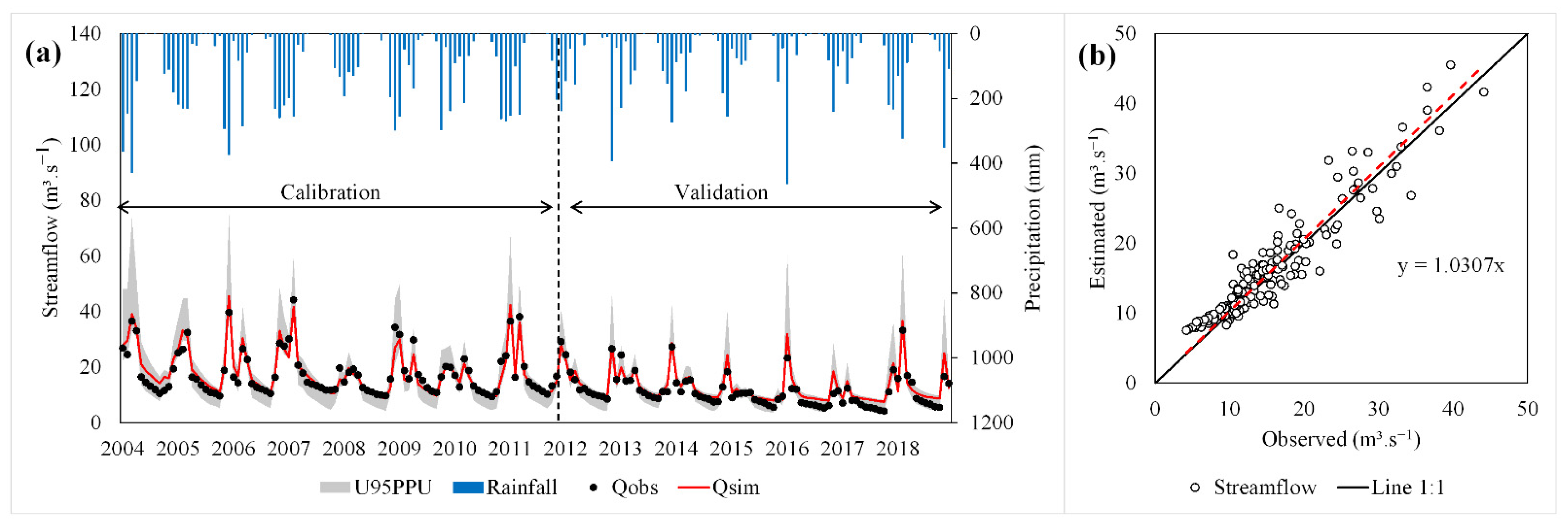
3.2. Calibration, Validation, and Uncertainty Analysis

Ten parameters were used in the SWAT calibration and validation with OP and CRU climatological data, selected based on previous studies in the PRB [56]. The final range and the best parameters obtained in the calibration (

Table 3. Parameters used to calibrate the SWAT model with OP and CRU climatological data and their initial and final ranges, and best parameters (BP).

Parameters	Description	Initial Range		Final Range		BP
r_CN2.mgt	SCS runoff Curve Number for moisture condition II	−0.100	0.100	−0.100	0.002	−0.090
v_ALPHA_BF.gw	Baseflow alpha factor	0.0050	0.0100	0.0050	0.0078	0.0051
a_GW_DELAY.gw	Groundwater delay	0.00	60.00	22.72	60.00	50.09
a_GWQMN.gw	Threshold depth of water in the shallow aquifer required for return flow to occur	0	2000	0	1208	925
v_CH_K2.rte	Effective hydraulic conductivity in main channel alluvium	0.00	20.00	5.92	17.78	14.27
v_GW_REVAP.gw	Groundwater “revap” coefficient	0.020	0.200	0.109	0.200	0.190
r_SLSUBBSN.hru	Average slope length	0.00	1.00	0.39	1.00	0.78
v_RCHRG_DP.gw	Deep aquifer percolation fraction	0.000	0.200	0.093	0.200	0.198
v_CH_K1.sub	Effective hydraulic conductivity in tributary channel alluvium	0.00	20.00	0.00	12.48	2.86
v_CH_N2.rte	Manning’s “n” value for the main channel	0.000	0.300	0.149	0.300	0.259

) agree with the result obtained by Junqueira et al. [65] in the same basin using OP and observed climatological data from 2004 to 2018. However, there are divergences such as RECHG_DP (deep aquifer percolation fraction) and CH_K1 (effective hydraulic conductivity in tributary channel alluvium), which showed best values equal to 0.050 and 11.44 mm.h⁻¹, respectively, in the previous study.

Figure 2 presents the simulated streamflow in the calibration and validation using the best parameters and the 95PPU with OP and CRU climatological data (from 2004 to 2018) and the scatter plots of observed and simulated streamflow. In addition,

Table 4. Results of uncertainty and performance analysis of SWAT for the calibration and validation with OP and CRU climate data.

	p-Factor	r-Factor	NSE	LNSE	PBIAS (%)	KGE
Calibration	0.98	1.29	0.89	0.88	−1.8	0.94
Validation	0.95	1.24	0.78	0.72	−12.7	0.85

presents the uncertainty analysis and performance results for the calibration and validation, expressed by the p-factor, r-factor, NSE, LNSE, PBIAS, and KGE.

The hydrological modeling showed low uncertainty during the calibration, with a p-factor close to 1 and r-factor less than 1.5, as recommended by Abbaspour et al. [55]. This result can be confirmed by Figure 2a, where it is observed that the 95PPU presented a small band covering most of the observed data. Regarding the performance of the hydrological modeling, NSE, LNSE, and PBIAS gave a result classified as “very good” according to the classification of Moriasi et al. [59]. In addition, the KGE close to 1 indicates a high fit between the simulated and observed data.

In the validation phase, there was a reduction in the r-factor, which caused a reduction in the p-factor. Abbaspour et al. [55] suggest that there should be a balance between the two factors. Therefore, there is no difference between the calibration and validation phases’ uncertainty. However, the performance of the hydrological simulation in the validation was worsened with a decrease in NSE, LNE, and KGE and an increase in PBIAS (in absolute values).

According to Junqueira et al. [33], an intense hydrological drought from 2013 to 2018 affected the basin, reducing the average streamflow rate by more than 50%. This drought can be related to the most significant overestimation of the simulated streamflow in the validation, since the hydrological conditions were distinct during the calibration period. This behavior was also observed in the scatter plot (Figure 2b), where there was an overestimation of the lowest observed streamflow, which occurred during the drought years’ recession period. Despite that, there was a satisfactory performance of the hydrological modeling. The year 2008 was also considered a drought year; however, the reduction in minimum streamflow was not as large as in 2013 to 2018 due to its shorter duration. Thus, the model did not present difficulty in representing the streamflow in 2008.

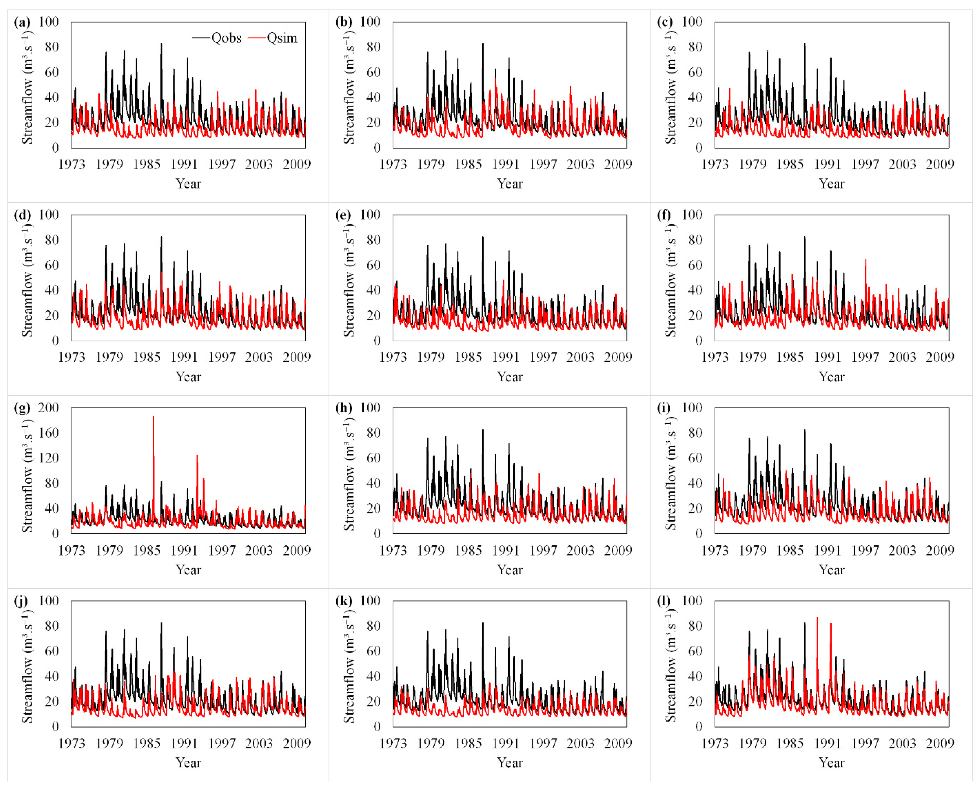
3.3. Hydrological Validation Based on Reanalysis Products

The hydrological modeling validation using precipitation products of climate reanalysis and CRU climate data was performed from August 1973 to December 2010 (Figure 3). Additionally,

Table 5. Statistical results of hydrological validation with the ten ERA-20CM ensemble members, the AE, and the ERA5-Land from August 1973 to December 2010 in monthly time scale to PRB.

Statistic	ERA-20CM Ensemble Members										AE	ERA5-Land
	Ens0	Ens1	Ens2	Ens3	Ens4	Ens5	Ens6	Ens7	Ens8	Ens9
NSE	−0.41	−0.25	−0.47	−0.09	−0.31	−0.24	−1.08	−0.34	−0.16	−0.50	−0.42	0.62
LNSE	−0.86	−0.61	−1.04	−0.24	−0.63	−0.34	−0.66	−0.74	−0.48	−1.12	−0.92	0.47
PBIAS (%)	29.6	24.6	34.4	18.5	31.3	18.6	14.3	30.6	27.5	31.1	38.6	20.0
KGE	0.20	0.32	0.21	0.37	0.28	0.29	0.07	0.26	0.38	0.19	0.25	0.75

presents the statistical results of the validation with the different products.

All reanalysis products were able to simulate the seasonal behavior of the streamflow (Figure 3); however, some divergences are observed. The ERA5-Land was the only reanalysis product to show satisfactory results, i.e., NSE > 0.5 and a PBIAS ranging from ± 25% [59]. Despite this, the LNSE was found to be unsatisfactory (<0.5) [59], a result influenced by the greater underestimation of streamflow in the early 1970s. In addition, the KGE was greater than 0.6, considered good according to Tarek et al. [10]. These results corroborate with the precipitation validation, where the ERA5-Land presented accumulated precipitation values closer to OP and better statistics on a daily and monthly scale.

Approximately 68.6% of the observed streamflow is covered by the range of simulated streamflow with the ten ERA-20CM ensemble members, with no difference between the rainy and dry periods (68.9% and 68.3%, respectively). However, the performance of these products was unsatisfactory, according to the classifications of Moriasi et al. [59] and Tarek et al. [10]. Correa et al. [14] also found unsatisfactory performance with ERA-20CM applied to hydrological modeling in the Amazon basin (average of ~20% against 27 gauge observations).

Overall, the performance in the validation with all products improved from the beginning of the 1990s. This probably occurred due to the bias correction of precipitation, which was performed with four rain gauges from the beginning of their data, being the first in 1981, the second in 1993, and the last two in 2000. Bias correction, according to a study of Correa et al. [17], improved the performance of hydrological modeling in the Amazon basin using ERA-20CM. In addition, the uncertainty of the model estimates is higher for the older period due to a smaller number of observations available to create an atmospheric forcing of adequate quality [12]. A similar situation occurs with the CRU data estimate, where the availability of observed data is low at the beginning of the 20th century in Brazil and increases over the years [43].

Another possible cause for the underestimation of the simulated streamflow at the beginning of the validation was a shift in the climatic regime around the 1970s, which generated a general increase in extreme precipitation events worldwide [66]. In South America, Jacques-Coper and Garreaud [67] found positive anomalies in precipitation in subtropical regions in the mid-1970s. These changes may not have been completely captured by climate reanalysis models and impacted hydrological modeling in the 1970s.

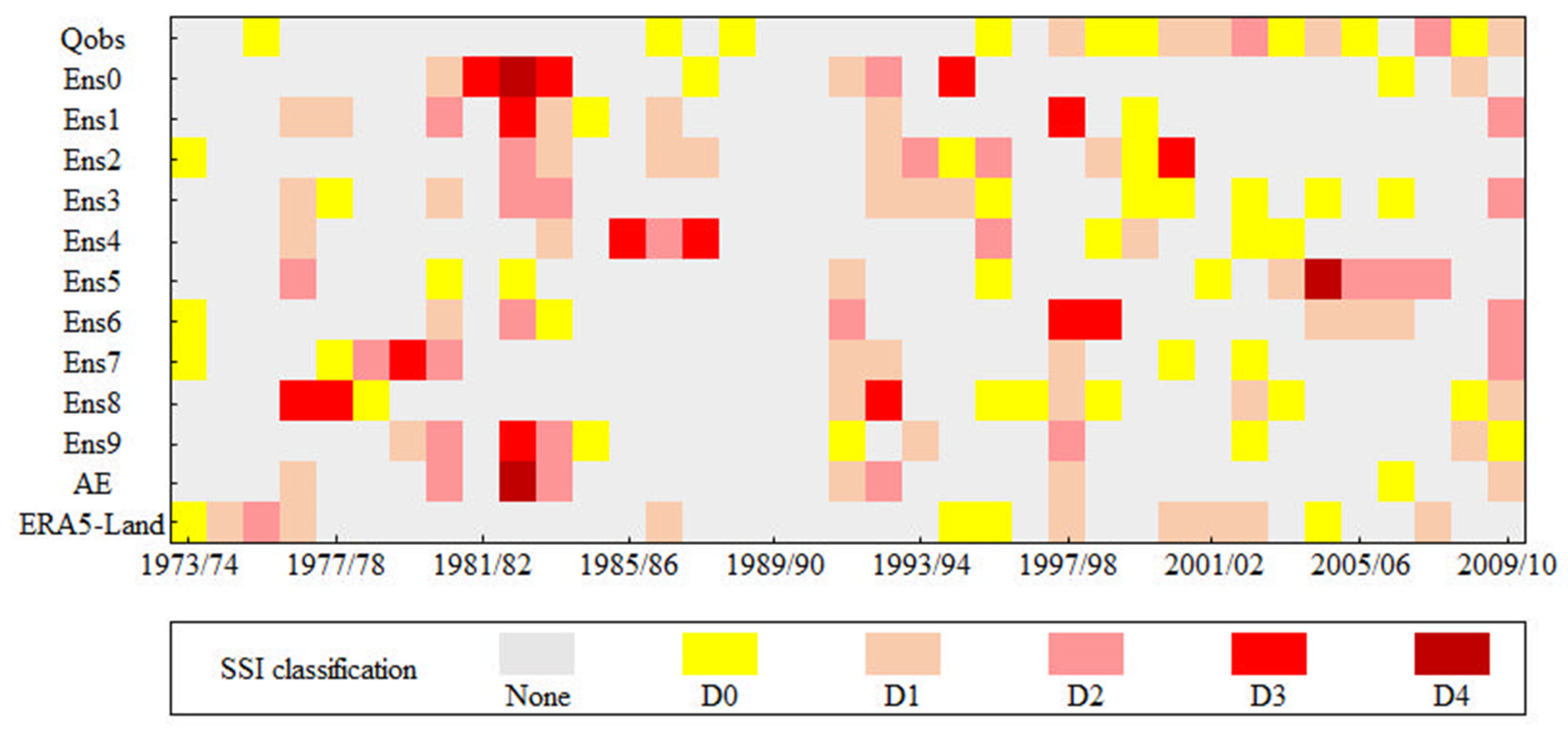
3.4. Drought Analysis

The Kolmogorov–Smirnov test (α = 0.05) indicated the suitability of the Gamma PDF for all products. Therefore, the SSI was calculated for the observed and simulated streamflow, as shown in Figure 4.

The main observed hydrological drought events occurred in 1997/98, 2000/01 to 2002/03, 2004/05, 2007/08, and 2009/10, all in the second half of the time series. In addition, abnormally dry years were observed in 1975/76, 1986/87, 1988/89, 1995/96, 1998/99, 1999/00, 2003/04, 2005/06, and 2008/09, and most of them occurred after drought years. From 1997/98 to 2009/10 only the year 2006/07 was not considered as drought or abnormally dry, with SSI equal to −0.19.

ERA5-Land was the reanalysis product that presented the best capacity to represent the hydrological drought occurrence in the basin, reflecting the best performance of this product in precipitation estimation and hydrological modeling. The ERA5-Land setup could predict five of the seven observed hydrological drought years from 1973 to 2010, representing 71.4% of the total events.

The longest hydrological drought that affected the basin occurred from 2000/01 to 2002/03, with severity equal to 3.72. The SSI based on the ERA5-Land setup was able to correctly estimate the duration (three years) and severity (3.11) of the drought in this period. On the other hand, the SSI based on ERA-20CM products did not provide an appropriate estimate of the drought in this period.

Among the ten ERA-20CM ensemble members, Ens6 and Ens8 showed a better ability to represent drought compared to the other members, with 42.9% of coincidence (1997/98, 2002/03, and 2009/10). However, Ens6 overestimated the drought intensity in two of the three events. Ens0 and Ens4 setups could not capture any drought events in the basin. On the other hand, Correa et al. [17], using data assimilation techniques and different approaches for bias correction, report that ERA-20CM was able to capture extreme events in the Amazon basin. Although AE performed better in estimating precipitation than the ERA20CM members individually, it was not able to perform an acceptable hydrological simulation and, consequently, a satisfactory simulation of drought years.

Pearson’s correlation coefficient indicates an adequate fit of the estimated SSI based on ERA5-Land to the observed SSI (r = 0.82), while the SSI calculated based on the ERA-20CM products showed a low correlation to the observed SSI (r < 0.2). This result indicates the better ability of ERA5-Land to simulate drought, wet, and average periods.

Although ERA5-Land has a shorter historical series than ERA-20CM, the performance was superior in all analyses conducted. Thus, ERA5-Land should be considered in hydrological studies that require long precipitation time series in the Brazilian savanna.

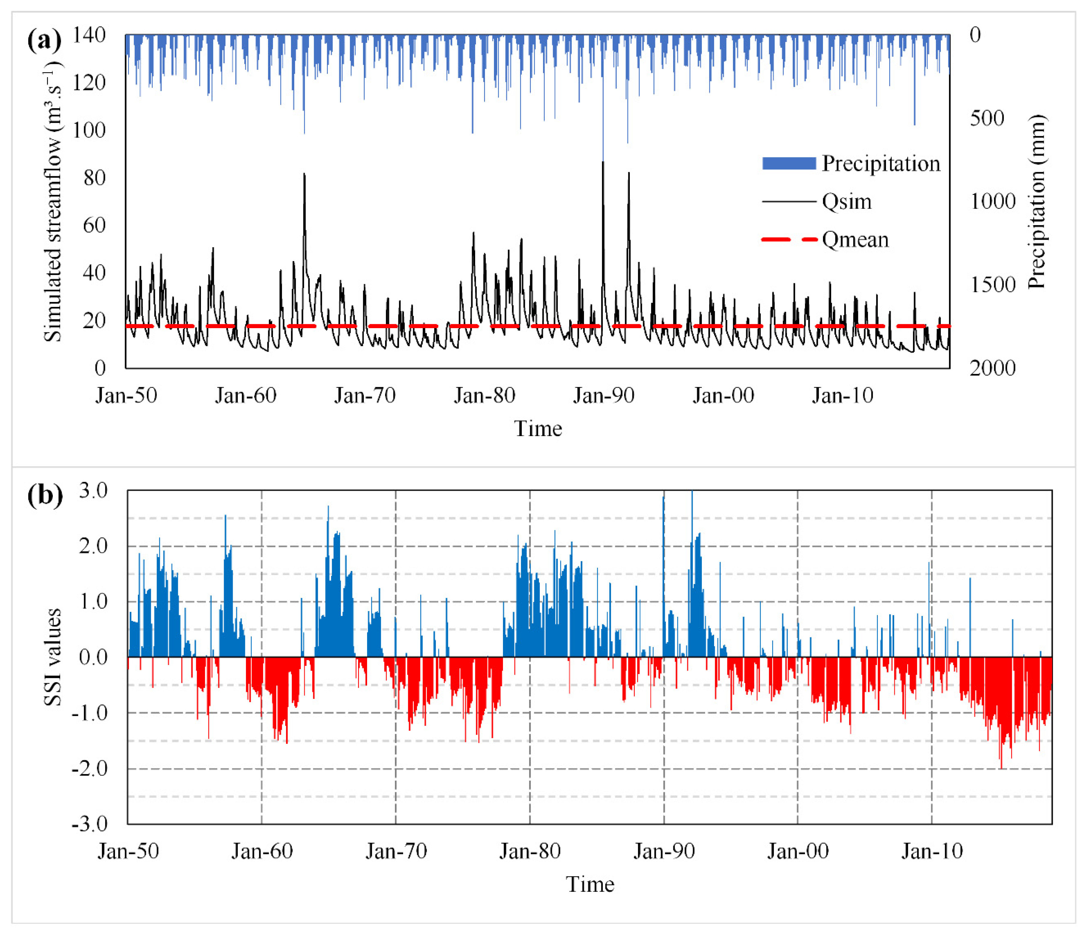
3.5. Hydrological Retrospective (HR) and Historical Droughts

Based on results obtained in the precipitation validation, hydrological modeling, and drought analysis, the HR was developed using ERA5-Land precipitation data and CRU climate data from January 1950 to December 2018 (Figure 5a). The inter- and intra-annual behavior of the simulated streamflow was similar to the behavior of the basin-scale precipitation, which shows the model’s capacity to simulate the streamflow in different meteorological conditions, such as wet and dry periods.

The most severe and most extended droughts that hit the PRB from 1950 to 2018 occurred in 1958/62, 1970/72, 1974/77, 2001/03, and 2012/18 (Figure 5b), although there were some non-drought months within these events. Other Brazilian regions also experienced drought events in some of these years, such as the state of Ceará in 1958 and 2012/18 [68]; Northeastern Brazil in 1958, 1970, 1976, 2001/02, and 2012/16 [69]; São Paulo city in 1962/63 and the metropolitan region of Belo Horizonte in 1970/71 [70], both in Southeastern Brazil; in the Doce River basin in 2000/01 and 2013/17 [71], Southeastern Brazil; and the Tocantins River basin from 2015 to 2017 [28], located in the Brazilian savanna; this confirms the adopted procedure’s ability to represent the most relevant droughts.

In 2001, a severe drought hit a large part of the Southeastern Brazilian region, resulting in a national energy crisis due to the reduction in the reservoir level of hydropower plants [72]. The drought of the last decade was one of the most severe in recent years in several basins in Brazil, causing impacts on agricultural production, hydropower generation, and over the environment [28,65,68,73]. From 2012 to 2016, 33.4 million people were affected by the droughts in Brazil, with estimated damage of BRL 104 billion (approximately USD 20 billion) [69]. Cuartas et al. [73] and Junqueira et al. [28] report that, in addition to reduced precipitation, temperature increases have intensified the drought conditions in basins located in the Brazilian savanna. Junqueira et al. [33] highlight that there was a 1.3 °C increase in temperature from 2013 to 2018 in the PRB, resulting in an increase in the evapotranspiration rate from 81.4% to 88.4%.

Overall, 294 months presented SSI values classified as drought or abnormally dry, of which 51.7% occurred in the last third of the period (1996–2018), behavior also observed in other studies of hydrological drought in Brazil [65,71,73]. Consequently, this period from 1996 to 2018 displayed the lowest number of months with SSI ≥ 0.5, only 7.9% of the total. Oliveira et al. [20] found a significant increase in evapotranspiration across the Brazilian savanna in recent years, which may have contributed to the higher frequency and intensity of droughts. According to Junqueira et al. [28], recent droughts have generated a reduction in the aquifer recharge and in the reservoir level in the Tocantins River basin, Brazilian savanna, negatively affecting the hydropower production. In addition, Ribeiro et al. [74] report a reduction in soil moisture and primary productivity in the Brazilian savanna in recent years. On the other hand, the second third of the period (1973–1995) showed a high incidence of wet months (47.9% of the total) and a low incidence of drought months (20.1%). Therefore, there has been an increase in droughts and a reduction in wet periods (precipitation above average) in recent decades.

Considering only the periods when the SSI was less than −0.5, the longest and most severe drought occurred from January 2014 to December 2015, totaling 24 months of duration and severity equal to 32.57, followed by the drought from April 1960 to December 1961, with a duration of 21 months and severity of 21.77, and by the drought from March 2017 to January 2018 (11 months), with a severity of 12.53. Therefore, there is a strong correlation between drought duration and severity, as observed by [75], i.e., the longer the duration of the drought, the greater its severity. This result is confirmed by Pearson’s correlation coefficient between drought severity and duration (r = 0.96). A similar analysis was conducted by Shiau [76] at a rain gauge station in Southern Taiwan, who found a correlation of 0.756.

4. Conclusions

ERA5-Land performed better in the precipitation validation for daily and monthly time scales when compared to ERA-20CM, with superior results in all statistics (r, RMSE, and KGE). Among the ERA-20CM products, AE performed better than the ten ERA-20CM ensemble members, especially on a monthly scale.

In hydrological modeling, ERA5-Land was the only product to show satisfactory performance in most statistics, following the criteria of Moriasi et al. [61] and Tarek et al. [10] (NSE = 0.62, LNSE = 0.47, PBIAS = 20.0%, and KGE = 0.75). On the other hand, the ERA-20CM ensemble members and the AE showed unsatisfactory performance in most statistics. A similar result was obtained in the drought analysis, where ERA5-Land simulated five out of seven drought events from 1973 to 2010. Therefore, ERA5-Land was able to simulate past streamflow and hydrological droughts.

The main historical drought events occurred in 1958/62, 1970/72, 1974/77, 2001/03, and 2012/18, with most of the months classified as drought or abnormally dry (51.7% of the total) occurring in the last third of the historical series (1996–2018). In addition, there was a reduction in the months with excess precipitation in the final third of the historical series (only 7.9% of the total).

References

1. Uniyal, B.; Dietrich, J.; Vu, N.Q.; Jha, M.K.; Arumí, J.L. Simulation of regional irrigation requirement with SWAT in different agro-climatic zones driven by observed climate and two reanalysis datasets. Sci. Total Environ. 2019, 649, 846–865. [Google Scholar] [CrossRef] [PubMed]
2. Gadelha, A.N.; Hugo, V.; Coelho, R.; Xavier, A.C.; Romero, L.; Melo, D.C.D.; Xuan, Y.; Hu, G.J.; Petersen, W.A.; Almeida, N. Grid box-level evaluation of IMERG over Brazil at various space and time scales. Atmos. Res. 2019, 218, 231–244. [Google Scholar] [CrossRef] [Green Version]
3. Xavier, A.C.; King, C.W.; Scanlon, B.R. Daily gridded meteorological variables in Brazil (1980–2013). Int. J. Climatol. 2016, 36, 2644–2659. [Google Scholar] [CrossRef] [Green Version]
4. Rozante, J.R.; Vila, D.A.; Chiquetto, J.B.; Fernandes, A.d.A.; Alvim, D.S. Evaluation of TRMM/GPM Blended Daily Products over Brazil. Remote Sens. 2018, 10, 882. [Google Scholar] [CrossRef] [Green Version]
5. Dee, D.P.; Balmaseda, M.; Balsamo, G.; Engelen, R.; Simmons, A.J.; Thépaut, J.-N. Toward a consistent reanalysis of the climate system. Bull. Am. Meteorol. Soc. 2014, 95, 1235–1248. [Google Scholar] [CrossRef]
6. Auerbach, D.A.; Easton, Z.M.; Walter, M.T.; Flecker, A.S.; Fuka, D.R. Evaluating weather observations and the Climate Forecast System Reanalysis as inputs for hydrologic modelling in the tropics. Hydrol. Process. 2016, 30, 3466–3477. [Google Scholar] [CrossRef]
7. IPCC. Climate Change 2013: The Physical Science Basis. Contribution of Working Group I to the Fifth Assessment Report of the Intergovernmental Panel on Climate Change; Stocker, T.F., Qin, D., Plattner, G.-K., Tignor, M., Allen, S.K., Boschung, J., Nauels, A., Xia, Y., Bex, V., Midgley, P.M., Eds.; Cambridge University Press: Cambridge, UK; New York, NY, USA, 2013.
8. Kim, D.-I.; Han, D. Evaluation of ERA-20cm reanalysis dataset over South Korea. J. Hydro-Environ. Res. 2019, 23, 10–24. [Google Scholar] [CrossRef]
9. Gao, L.; Bernhardt, M.; Schulz, K.; Chen, X.; Chen, Y.; Liu, M. A first evaluation of ERA-20CM over China. Mon. Weather Rev. 2016, 144, 45–57. [Google Scholar] [CrossRef]
10. Tarek, M.; Brissette, F.P.; Arsenault, R. Evaluation of the ERA5 reanalysis as a potential reference dataset for hydrological modelling over North America. Hydrol. Earth Syst. Sci. 2020, 24, 2527–2544. [Google Scholar] [CrossRef]
11. Hersbach, H.; Peubey, C.; Simmons, A.; Berrisford, P.; Poli, P.; Dee, D. ERA-20CM: A twentieth-century atmospheric model ensemble. Q. J. R. Meteorol. Soc. 2015, 141, 2350–2375. [Google Scholar] [CrossRef]
12. Muñoz-Sabater, J.; Dutra, E.; Agustí-Panareda, A.; Albergel, C.; Arduini, G.; Balsamo, G.; Boussetta, S.; Choulga, M.; Harrigan, S.; Hersbach, H.; et al. ERA5-Land: A state-of-the-art global reanalysis dataset for land applications. Earth Syst. Sci. Data 2021, 13, 4349–4383. [Google Scholar] [CrossRef]
13. Slivinski, L.C.; Compo, G.P.; Whitaker, J.S.; Sardeshmukh, P.D.; Giese, B.S.; McColl, C.; Allan, R.; Yin, X.; Vose, R.; Titchner, H.; et al. Towards a more reliable historical reanalysis: Improvements for version 3 of the Twentieth Century Reanalysis system. Q. J. R. Meteorol. Soc. 2019, 145, 2876–2908. [Google Scholar] [CrossRef] [Green Version]
14. Correa, S.W.; de Paiva, R.C.D.; Espinoza, J.C.; Collischonn, W. Multi-decadal Hydrological Retrospective: Case study of Amazon floods and droughts. J. Hydrol. 2017, 549, 667–684. [Google Scholar] [CrossRef] [Green Version]
15. Jajarmizadeh, M.; Sidek, L.M.; Mirzai, M.; Alaghmand, S.; Harun, S.; Majid, M.R. Prediction of Surface Flow by Forcing of Climate Forecast System Reanalysis Data. Water Resour. Manag. 2016, 30, 2627–2640. [Google Scholar] [CrossRef]
16. Alfieri, L.; Lorini, V.; Hirpa, F.A.; Harrigan, S.; Zsoter, E.; Prudhomme, C.; Salamon, P. A global streamflow reanalysis for 1980–2018. J. Hydrol. X 2020, 6, 100049. [Google Scholar] [CrossRef] [PubMed]
17. Correa, S.W.; Paiva, R.C.D.; Siqueira, V.; Collischonn, W. Hydrological reanalysis across the 20th century: A case study of the Amazon Basin. J. Hydrol. 2019, 570, 755–773. [Google Scholar] [CrossRef]
18. Colli, G.R.; Vieira, C.R.; Dianese, J.C. Biodiversity and conservation of the Cerrado: Recent advances and old challenges. Biodivers. Conserv. 2020, 29, 1465–1475. [Google Scholar] [CrossRef] [Green Version]
19. Myers, N.; Mittermeier, R.A.; Mittermeier, C.G.; da Fonseca, G.A.B.; Kent, J. Biodiversity hotspots for conservation priorities. Nature 2000, 403, 853–858. [Google Scholar] [CrossRef]
20. Oliveira, P.T.S.; Nearing, M.A.; Moran, M.S.; Goodrich, D.C.; Wendland, E.; Gupta, H.V. Trends in water balance components across the Brazilian Cerrado. Water Resour. Res. 2014, 50, 7100–7114. [Google Scholar] [CrossRef] [Green Version]
21. Kim, D.-I.; Kwon, H.; Han, D. Exploring the Long-Term Reanalysis of Precipitation and the Contribution of Bias Correction to the Reduction of Uncertainty over South Korea: A Composite Gamma-Pareto Distribution Approach to the Bias Correction. Hydrol. Earth Syst. Sci. Discuss. 2018, 1–53. [Google Scholar] [CrossRef] [Green Version]
22. Smith, K.A.; Barker, L.J.; Tanguy, M.; Parry, S.; Harrigan, S.; Legg, T.P.; Prudhomme, C.; Hannaford, J. A multi-objective ensemble approach to hydrological modelling in the UK: An application to historic drought reconstruction. Hydrol. Earth Syst. Sci. 2019, 23, 3247–3268. [Google Scholar] [CrossRef] [Green Version]
23. Van Loon, A.F. Hydrological drought explained. Wiley Interdiscip. Rev. Water 2015, 2, 359–392. [Google Scholar] [CrossRef]
24. Hasan, H.H.; Razali, S.F.M.; Muhammad, N.S.; Ahmad, A. Research trends of hydrological drought: A systematic review. Water 2019, 11, 2252. [Google Scholar] [CrossRef] [Green Version]
25. Zhang, X.; Chen, N.; Sheng, H.; Ip, C.; Yang, L.; Chen, Y.; Sang, Z.; Tadesse, T.; Lim, T.P.Y.; Rajabifard, A.; et al. Urban drought challenge to 2030 sustainable development goals. Sci. Total Environ. 2019, 693, 133536. [Google Scholar] [CrossRef] [PubMed]
26. Amorim, J.d.S.; Viola, M.R.; Junqueira, R.; de Mello, C.R.; Bento, N.L.; Avanzi, J.C. Quantifying the Climate Change-Driven Impacts on the Hydrology of a Data-Scarce Watershed Located in the Brazilian Tropical Savanna. Hydrol. Process. 2022, 36, 1–15. [Google Scholar] [CrossRef]
27. Rodrigues, J.A.M.; Viola, M.R.; Alvarenga, L.A.; Mello, C.R.; Chou, S.C.; Oliveira, V.A.; Uddameri, V.; Morais, M.A.V. Climate change impacts under representative concentration pathway scenarios on streamflow and droughts of basins in the Brazilian Cerrado biome. Int. J. Climatol. 2019, 40, 2511–2526. [Google Scholar] [CrossRef]
28. Junqueira, R.; Viola, M.R.; de Mello, C.R.; Vieira-Filho, M.; Alves, M.V.G.; Amorim, J.D.S. Drought severity indexes for the Tocantins River Basin, Brazil. Theor. Appl. Climatol. 2020, 141, 465–481. [Google Scholar] [CrossRef]
29. IBGE-Instituto Brasileiro de Geografia e Estatística. Biomas e Sistema Costeiro-Marinho do Brasil-1:250.000; IBGE, Coordenação de Recursos Naturais e Estudos Ambientais: Rio de Janeiro, Brazil, 2019; pp. 125–138.
30. Nunes, Y.R.F.; Azevedo, I.F.P.; Neves, W.V.; Veloso, M.d.D.M.; Souza, R.D.A.; Fernandes, G.W. Pandeiros: O Pantanal Mineiro. MG. Biota 2009, 2, 4–17. [Google Scholar]
31. Santos, U.; Silva, P.C.; Barros, L.C.; Dergam, J.A. Fish fauna of the Pandeiros River, a region of environmental protection for fish species in Minas Gerais state, Brazil. Check List 2015, 11, 1507. [Google Scholar] [CrossRef] [Green Version]
32. Martins, F.B.; Gonzaga, G.; Dos Santos, D.F.; Reboita, M.S. Classificação climática de Köppen e de Thornthwaite para Minas Gerais: Cenário atual e projeções futuras. Rev. Bras. Climatol. 2018, 1, 149–164. [Google Scholar] [CrossRef] [Green Version]
33. Junqueira, R.; Viola, M.R.; Amorim, J.d.S.; Mello, C.R. De Hydrological Response to Drought Occurrences in a Brazilian Savanna Basin. Resources 2020, 9, 123. [Google Scholar] [CrossRef]
34. Ambrizzi, T.; Ferraz, S.E.T. An objective criterion for determining the South Atlantic convergence zone. Front. Environ. Sci. 2015, 3, 23. [Google Scholar] [CrossRef] [Green Version]
35. Prado, L.F.; Wainer, I.; Yokoyama, E.; Khodri, M.; Garnier, J. Changes in summer precipitation variability in central Brazil over the past eight decades. Int. J. Climatol. 2021, 41, 4171–4186. [Google Scholar] [CrossRef]
36. Arnold, J.G.; Srinivasan, R.; Muttiah, R.S.; Williams, J.R. Large area hydrologic modeling and assessment part I: Model development. J. Am. Water Resour. Assoc. 1998, 34, 73–89. [Google Scholar] [CrossRef]
37. Neitsch, S.L.; Arnold, J.G.; Kiniry, J.R.; Grassland, W.J.R. Soil & Water Assessment Tool Theoretical Documentation: Version 2009; Texas Water Resources Institute: Forney, TX, USA, 2011. [Google Scholar]
38. Gassman, P.W.; Reyes, M.R.; Green, C.H.; Arnold, J.G. The soil and water assessment tool: Historical development, applications, and future research directions. Trans. ASABE 2007, 50, 1211–1250. [Google Scholar] [CrossRef] [Green Version]
39. Soil Conservation Service (SCS). Section 4, Hydrology. In National Engineering Handbook; United States Department of Agriculture: Washington, DC, USA, 1972. [Google Scholar]
40. Monteith, J.L. Evaporation and environment. Symp. Soc. Exp. Biol. 1965, 19, 205–234. [Google Scholar] [PubMed]
41. Penman, H.L. Evaporation: An introductory survey. Neth. J. Agric. Sci. 1956, 4, 9–29. [Google Scholar] [CrossRef]
42. Williams, J.R. Flood Routing With Variable Travel Time or Variable Storage Coefficients. Trans. ASAE 1969, 12, 100–103. [Google Scholar] [CrossRef]
43. Harris, I.; Osborn, T.J.; Jones, P.; Lister, D. Version 4 of the CRU TS monthly high-resolution gridded multivariate climate dataset. Sci. Data 2020, 7, 109. [Google Scholar] [CrossRef] [Green Version]
44. Allen, R.G.; Pereira, L.S.; Raes, D.; Smith, M. FAO Irrigation and Drainage Paper No. 56-Crop Evapotranspiration; FFood and Agriculture Organization of the United Nations: Rome, Italy, 2006. [Google Scholar]
45. New, M.; Lister, D.; Hulme, M.; Makin, I. A high-resolution data set of surface climate over global land areas. Clim. Res. 2002, 21, 1–25. [Google Scholar] [CrossRef] [Green Version]
46. Haltiner, G.J.; Martin, F.L. Dynamic and Physical Meteorology. McGraw-Hill Book Company: New York, NY, USA, 1957. [Google Scholar]
47. FEAM-Fundação Estadual do Meio. Ambiente Mapa de solos do Estado de Minas Gerais; FEAM: Belo Horizonte, Brazil, 2010.
48. IBGE-Instituto Brasileiro de Geografia e Estatística. Mapa de Cobertura e Uso da Terra do Brasil 2010; IBGE: Rio de Jeneiro, Brazil, 2018.
49. Poli, P.; Hersbach, H.; Dee, D.P.; Berrisford, P.; Simmons, A.J.; Vitart, F.; Laloyaux, P.; Tan, D.G.H.; Peubey, C.; Thépaut, J.N.; et al. ERA-20C: An atmospheric reanalysis of the twentieth century. J. Clim. 2016, 29, 4083–4097. [Google Scholar] [CrossRef]
50. Hersbach, H.; Peubey, C.; Simmons, A.; Poli, P. ERA-20CM: A twentieth century atmospheric model ensemble. Report 2013, 46, 1–44. [Google Scholar] [CrossRef]
51. Muñoz-Sabater, J. ERA5-Land Hourly Data from 1981 to Present; Copernicus Climate Change Service Climate Data Store: Brussels, Belgium, 2019. [Google Scholar]
52. Muñoz-Sabater, J. ERA5-Land Hourly Data from 1950 to 1980; Copernicus Climate Change Service Climate Data Store: Brussels, Belgium, 2021. [Google Scholar]
53. Lenderink, G.; Buishand, A.; van Deursen, W. Estimates of future discharges of the river Rhine using two scenario methodologies: Direct versus delta approach. Hydrol. Earth Syst. Sci. 2007, 11, 1145–1159. [Google Scholar] [CrossRef]
54. Teutschbein, C.; Seibert, J. Bias correction of regional climate model simulations for hydrological climate-change impact studies: Review and evaluation of different methods. J. Hydrol. 2012, 456–457, 12–29. [Google Scholar] [CrossRef]
55. Abbaspour, K.C.; Rouholahnejad, E.; Vaghefi, S.; Srinivasan, R.; Yang, H.; Kløve, B. A continental-scale hydrology and water quality model for Europe: Calibration and uncertainty of a high-resolution large-scale SWAT model. J. Hydrol. 2015, 524, 733–752. [Google Scholar] [CrossRef] [Green Version]
56. Junqueira, R.; Viola, M.R.; Amorim, J.d.S.; Camargos, C.; de Mello, C.R. Hydrological modeling using remote sensing precipitation data in a Brazilian savanna basin. J. South Am. Earth Sci. 2022, 115, 103773. [Google Scholar] [CrossRef]
57. Abbaspour, K.C. SWAT-CUP: SWAT Calibration and Uncertainty Programs; Swiss Federal Institute of Aquatic Science and Technology: Dübendorf, Switzerland, 2015. [Google Scholar]
58. Nogueira, S.M.C.; Moreira, M.A.; Volpato, M.M.L. Evaluating precipitation estimates from Eta, TRMM and CHRIPS data in the south-southeast region of Minas Gerais state-Brazil. Remote Sens. 2018, 10, 313–329. [Google Scholar] [CrossRef] [Green Version]
59. Moriasi, D.N.; Arnold, J.G.; Van Liew, M.W.; Bingner, R.L.; Harmel, R.D.; Veith, T.L. Model Evaluation Guidelines for Systematic Quantification of Accuracy in Watershed Simulations. Trans. ASABE 2007, 50, 885–900. [Google Scholar] [CrossRef]
60. Vicente-Serrano, S.M.; López-Moreno, J.I.; Beguería, S.; Lorenzo-Lacruz, J.; Azorin-Molina, C.; Morán-Tejeda, E. Accurate Computation of a Streamflow Drought Index. J. Hydrol. Eng. 2012, 17, 318–332. [Google Scholar] [CrossRef] [Green Version]
61. Svoboda, M.; LeComte, D.; Hayes, M.; Heim, R.; Gleason, K.; Angel, J.; Rippey, B.; Tinker, R.; Palecki, M.; Stooksbury, D.; et al. The drought monitor. Bull. Am. Meteorol. Soc. 2002, 83, 1181–1190. [Google Scholar] [CrossRef] [Green Version]
62. Yevjevich, V.M. Objective Approach to Definitions and Investigations of Continental Hydrologic Droughts. Ph.D. Thesis, Colorado State University, Fort Collins, Colorado, 1967. [Google Scholar]
63. Gehne, M.; Hamill, T.M.; Kiladis, G.N.; Trenberth, K.E. Comparison of global precipitation estimates across a range of temporal and spatial scales. J. Clim. 2016, 29, 7773–7795. [Google Scholar] [CrossRef]
64. ECMWF. IFS Documentation CY45R1; ECMWF: Reading, UK, 2018. [Google Scholar]
65. Junqueira, R.; Amorim, J.d.S.; Viola, M.R.; De Mello, C.R.; Uddameri, V.; Prado, L.F. Drought occurrences and impacts on the upper Grande river basin, Brazil. Meteorol. Atmos. Phys. 2022, 134, 45. [Google Scholar] [CrossRef]
66. Sarkar, S.; Maity, R. Global climate shift in 1970s causes a significant worldwide increase in precipitation extremes. Sci. Rep. 2021, 11, 1–11. [Google Scholar] [CrossRef]
67. Jacques-Coper, M.; Garreaud, R.D. Characterization of the 1970s climate shift in South America. Int. J. Climatol. 2015, 35, 2164–2179. [Google Scholar] [CrossRef]
68. Pontes Filho, J.D.; Souza Filho, F.d.A.; Martins, E.S.P.R.; Studart, T.M.D.C. Copula-Based Multivariate Frequency Analysis of the 2012–2018 Drought in Northeast Brazil. Water 2020, 12, 834. [Google Scholar] [CrossRef] [Green Version]
69. Marengo, J.A.; Alves, L.M.; Alvala, R.C.S.; Cunha, A.P.; Brito, S.; Moraes, O.L.L. Climatic characteristics of the 2010-2016 drought in the semiarid northeast Brazil region. An. Acad. Bras. Cienc. 2018, 90, 1973–1985. [Google Scholar] [CrossRef] [PubMed]
70. Silva, V.O.; Mello, C.R. Meteorological droughts in part of southeastern Brazil: Understanding the last 100 years. An. Acad. Bras. Cienc. 2021, 93, 1–17. [Google Scholar] [CrossRef]
71. Jesus, E.T.; Amorim, J.S.; Junqueira, R.; Viola, M.R.; Mello, C.R. Meteorological and hydrological drought from 1987 to 2017 in Doce River Basin, Southeastern Brazil. Rev. Bras. Recur. Hídricos 2020, 25, 1–12. [Google Scholar] [CrossRef]
72. Marengo, J.A.; Alves, L.M. Crise Hídrica em São Paulo em 2014: Seca e Desmatamento. GEOUSP Espaço Tempo 2015, 19, 485. [Google Scholar] [CrossRef] [Green Version]
73. Cuartas, L.A.; Cunha, A.P.M.d.A.; Alves, J.A.; Parra, L.M.P.; Deusdará-Leal, K.; Costa, L.C.O.; Molina, R.D.; Amore, D.; Broedel, E.; Seluchi, M.E.; et al. Recent Hydrological Droughts in Brazil and Their Impact on Hydropower Generation. Water 2022, 14, 601. [Google Scholar] [CrossRef]
74. Ribeiro, F.L.; Guevara, M.; Vázquez-Lule, A.; Paula Cunha, A.; Zeri, M.; Vargas, R. The impact of drought on soil moisture trends across Brazilian biomes. Nat. Hazards Earth Syst. Sci. 2021, 21, 879–892. [Google Scholar] [CrossRef]
75. de Almeida, R.; Barbosa, P.S.F. Simulation of the occurrence of drought events via copulas. RBRH 2020, 25, 1–13. [Google Scholar] [CrossRef] [Green Version]
76. Shiau, J.T. Fitting Drought Duration and Severity with Two-Dimensional Copulas. Water Resour. Manag. 2006, 20, 795–815. [Google Scholar] [CrossRef]
Figure 1. Location of PRB and its DEM, hydrometeorological data, and soil and land use maps.
Water 14 02178 g001
Figure 2. (a) Average precipitation, observed (Qobs) and simulated (Qsim) monthly streamflow, and uncertainty band; (b) scatter plots of the observed and simulated monthly streamflow from January 2004 to December 2018.
Water 14 02178 g002
Figure 3. Hydrological validation with the ten ERA-20CM ensemble members (aj), AE (k), and the ERA5-Land (l) from August 1973 to December 2010 to PRB.
Water 14 02178 g003
Figure 4. SSI classification for the observed (Qobs) and simulated streamflow with the ten ERA-20CM ensemble members, the AE, and the ERA5-Land from 1973/74 to 2009/10 for the PRB, where D0 is “abnormally dry”, D1 is “moderate drought”, D2 is “severe drought”, D3 is “extreme drought”, and D4 is “exceptional drought”.
Water 14 02178 g004
Figure 5. HR (Qsim), mean streamflow (Qmean), and basin-scale precipitation (a); historical drought results for PRB from January 1950 to December 2018 (b), where blue columns represent SSI above 0 and red columns mean SSI below zero.
Water 14 02178 g005