
Study of Non-Point Pollution in the Ashe River Basin Based on SWAT Model with Different Land Use


School of Hydraulic and Electric Power, Heilongjiang University, Harbin 150080, China
*
Author to whom correspondence should be addressed.
Water 2022, 14(14), 2177; https://doi.org/10.3390/w14142177
Submission received: 9 June 2022
/
Revised: 7 July 2022
/
Accepted: 7 July 2022
/
Published: 10 July 2022
(This article belongs to the Special Issue Water Quality Changes of Lakes and Rivers)
Abstract
:The Ashe River Basin (ARB), long known as the “Golden Waterway” in Manchu, has become one of China’s most polluted rivers. The basin area of the Ashe River is 3545 km2 and the total length of the river is 257 km. There have not been specific studies on land use change and non-point pollution in the ARB region. This paper uses the ARB watershed as the study area, simulates the watershed using the SWAT (Soil and Water Assessment Tool) model, and analyzes the hydrological processes and the temporal and spatial changes of total nitrogen and total phosphorus in the watershed with hydrology and water quality as the objectives under different periods of land use to reduce pollution in the watershed and protect the environment. The results show that the simulation of runoff, and even the R2 and NS (both the coefficient of determination and the Nash–Sutcliffe efficiency coefficient are simulated by SWAT-CUP, which is generally used to validate the simulation results of the hydrological model, where the closer the result is to 1, the better the effect) of total nitrogen and total phosphorus in the watershed, are also all above 0.75 and have good applicability during regular and validation periods. Since 2000, the simulated monthly average total nitrogen and total phosphorus levels have progressively grown. The most polluted areas are concentrated in the middle and lower reaches of the watershed near the main streams owing to the rise in load per unit area caused by the collection of pollutants from the upper watershed to the watershed outlet, and even an increase in fertilizer application due to the larger area of cultivated land.
1. Introduction
While water is a precious resource all around the world, pollution is today a significant cultural concern, limiting long-term economic growth. The most significant aspect of water pollution is non-point source pollution, which is the most complicated to control [1]. Because non-point source pollution is tightly tied to human activities and environmental elements such as soil, atmosphere, hydrology, and vegetation, it is difficult to monitor it for spatial and temporal changes [2]. Land use/cover change (LUCC) has a clear effect on the redistribution of water resources in spatial and temporal patterns, along with changes in the transport patterns of various pollutants mediated by water in watershed hydrology [3]. It also causes more ecological problems, such as water environment degradation, soil erosion, and land degradation, all of which have an impact on a society’s long-term sustainability [4]. Due to the progressive evolution of contemporary life, which has produced the fastest increasing population, expanding urbanization, and checks and balances on local production conditions, crop production has become one of the most challenging operations [5]. Changes in land management and consumer preferences had a tremendous impact on marine life, resulting in the progressive rise of water blooms and eutrophication that were previously absent [6].
The field monitoring method, emission factor method, and hydrological water quality modeling method are the three basic techniques for analyzing water pollution used across the world [7]. Field monitoring is essential in field monitoring methods, which results in increased labor intensity, high expense, and long periodicity, and often the precision of pollutant load cannot be predicted owing to a variety of factors such as information unavailability or low dependability [8]. Hydrological and water quality models have been widely applied in surface source contamination modeling in recent years [9].
The USDA in Tamburlaine, Texas and the Texas A&M University Research Office developed the Soil and Water Assessment Tool (SWAT), a watershed-scale ecohydrological model [10]. SWAT is a physical, chemical, and continuous time dynamic model that includes a variety of elements with physical and semi-empirical features. This model allows us to simulate the hydrological cycle in a watershed by inputting various spatial and attribute data such as changes in pollution sources, and to change a certain value to perform a simulation for pollution, so that certain solutions can be found [11].
Chanasyk et al. utilized the SWAT model to investigate the hydrology–soil interaction for various land use types and to determine the model’s functional properties for realistic simulation in watersheds with low rainfall [12]. Arnold et al. adapted the SWAT model in 1993 and applied it to the Montana watershed’s high elevation sector. Because of the high forest cover and unique geography of the area, snowmelt is the primary supply of water [13]. Wang et al. used the SWAT model to simulate spring snowmelt pollution sources in the Liao River’s source area and discovered that the SWAT model performs well in simulating seasonal non-point pollution with snowmelt. They also discovered that rainfall and snowmelt are the main drivers of non-point pollution in cold regions [14]. Shen et al. employed SWAT to estimate nitrogen and phosphorus loads in the Three Gorges Reservoir watershed and discovered that rice paddies and non-irrigated cropland were the most significant sources [15]. Einheuser et al. investigated nutrient concentrations in the Saginaw River and found that nutrient concentrations had the largest impact on river health, confirming that this combination can forecast river health as well as specify specific protection measures. Where the combination of conservation measures includes no-till, residual management, and native grasses, results suggest that nutrient concentrations have the strongest influence on all three macroinvertebrate measures. Consistently, average annual organic nitrogen showed the most significant association with EPTtaxa and HBI [16]. Thus, the SWAT model may be employed to its full potential in the area and produce good results [17].
A study in Thailand showed that in concepts of the land use study, it was realized that the environment of the site was prone to flooding and water quality deterioration during the period of drastic land use change, and that non-point source pollution increased with land use change in almost all spatial and temporal pollution loads [18]. Studies have also shown that farmland and grasslands are considered to be sources of pollution in cities, while forest vegetation improves water quality and is the best filter for pollutants compared to urban sources [19]. According to agricultural research, increased crop area and long-term fertilizer use from Dalyan led to a slight rise in nitrogen flow into rivers [20]. Experiments conducted in the Gachon watershed and the main watershed of the Kum-gang River in Korea showed that the reduction in agricultural land or the difference in management practices due to fertilizer application was accompanied by a reduction in nitrogen and phosphorus loads [21].
In the upper San Pedro River basin, urbanization was the most significant factor in increasing surface runoff and water production, while replacement of desert shrubs/grasses with herbs was the most significant factor in reducing baseflow/seepage and leading to increased evapotranspiration [22]. An increase in surface flow will reduce groundwater recharge. In changing the cultivation of agricultural land to vegetated grassland or forest, there is some possibility of reducing the frequency of flooding, but not necessarily the duration [23].
The Ashe River Basin (ARB) is a primary tributary of the right bank of the Songhua River and one of the biggest and best grain production bases, located close to Harbin, Heilongjiang Province [24]. The ARB has always had serious problems, such as low flood control standards, poor water environment, wasted water resources, and degraded social service functions, with rising food production and economy from upstream to downstream, from mountainous areas to cities, and from Class III water bodies to poor V water bodies in terms of China’s surface water environmental quality. In the Northeast, no studies on the combination of surface pollution and land use have been produced. Studies on runoff response are often applied, but the Ashe River Basin is generally investigated for hydrology, and no studies on point source pollution utilizing land use as a medium have been conducted [25].
This paper focuses on the ARB as the research object and evaluates the non-point pollution load of the ARB, as well as the nitrogen and phosphorus pollution load and spatial and temporal distribution pattern under extensive land use scenarios, by using SWAT non-point pollution model. It also serves as a foundation for technical techniques for controlling non-point pollution in the ARB, as well as supporting the protection of water resources and monitoring water pollution in the water source region.
2. Materials and Methods
2.1. Study Area
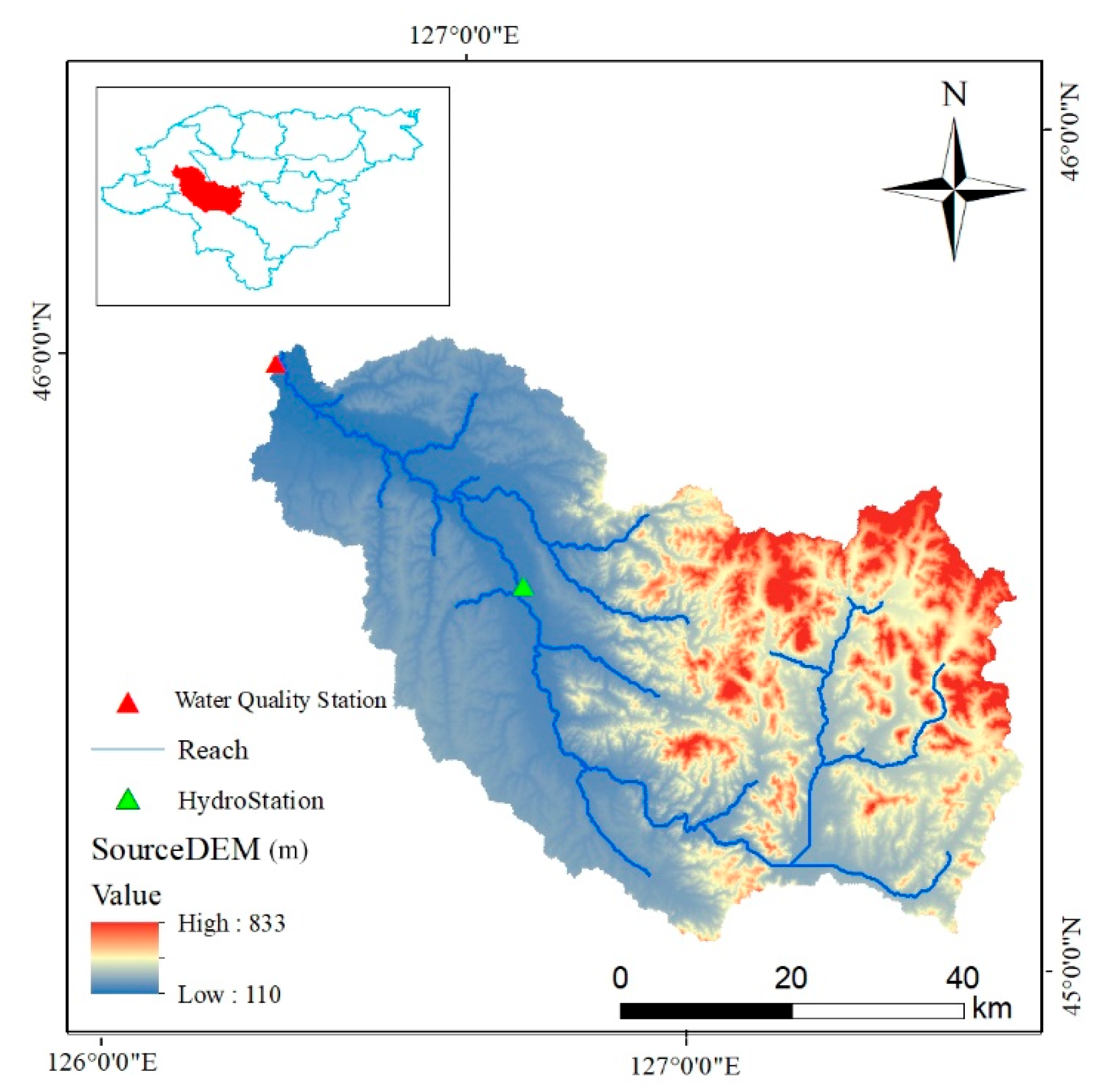
The Ashe River basin, which flows from Mount Maoer, is a primary tributary on the Songhua River’s right bank. The main stream of the Ashe River is 213 km long, with a basin area of 3545 km squared, as shown in Figure 1. The elevations in Figure 1 are in meters.
The Ashe River flows into the Songhua River from Shangzhi City, Wuchang City, Acheng District, and Harbin City, among other cities and counties, and the eastern suburbs of Harbin City. The river flows through Acheng District for 169 km, the upper reaches of the terrain have a large height difference, the river is fast, the river bed is narrow, the middle reaches have a medium height difference, the river bed is slightly wide, the water flow is slow, the downstream river bed is wide, and the river is curved.
The Ashe River is a mountainous stream that has abundant water in the summer but freezes in winter, relying primarily on mudflats for flooding.
The watershed has a continental monsoon climate; it has less rain and more drought in spring, and is warm and rainy in summer. In autumn, it is cooler in the morning and evening and is easy to frost, while in winter it is cold and easy to freeze. It is cooler in the mornings and evenings in autumn and prone to frost, and it is cold and prone to ice in winter.
The hydrological station shown in Figure 1 has the name of Acheng Station. It receives an average annual rainfall of 532 mm, with June to September receiving 75% of the annual rainfall. Spring and summer bring more southeast breezes, while autumn and winter bring more northwest winds. The maximum wind speed for the last year has been 37 m/s, while the average temperature has been 3.4 °C. The average multi-year extreme maximum temperature is 39.2 °C, the average multi-year extreme low temperature is −37.3 °C, and the average soil freezing depth is 1.7–2.0 m.
2.2. Data Collection
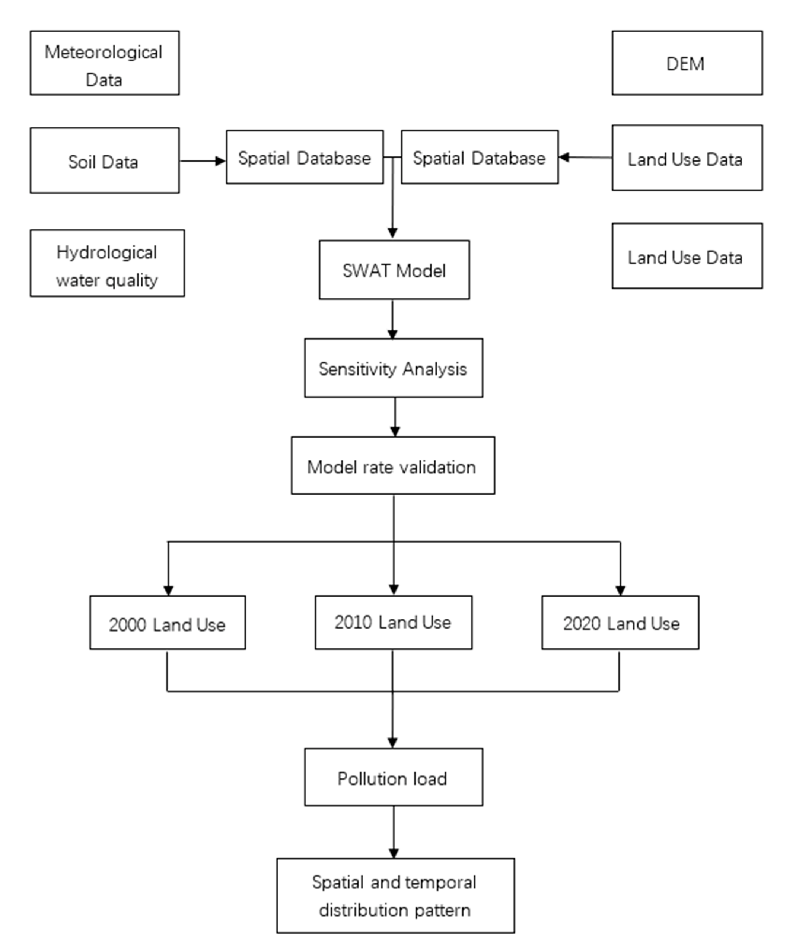
The SWAT model requires both spatial and attribute data. DEM (Digital Elevation Model), land use maps, soil type maps, and watershed hydrology maps are among some of the spatial data. More importantly, meteorological data are used to simulate the watershed model’s climate and precipitation sources. The coordinate system used in this paper is the WGS 1984. The projection coordinates are used in the UTM projection, which is called WGS 1984 UTM Zone 52° N because this geographical location of the Ashe River basin is between 126°40′ E 127°43′ E and 45°05′ N 45°50′ N. The following table lists the data sources and basic information needed for this paper (Table 1).
2.2.1. Watershed System Data
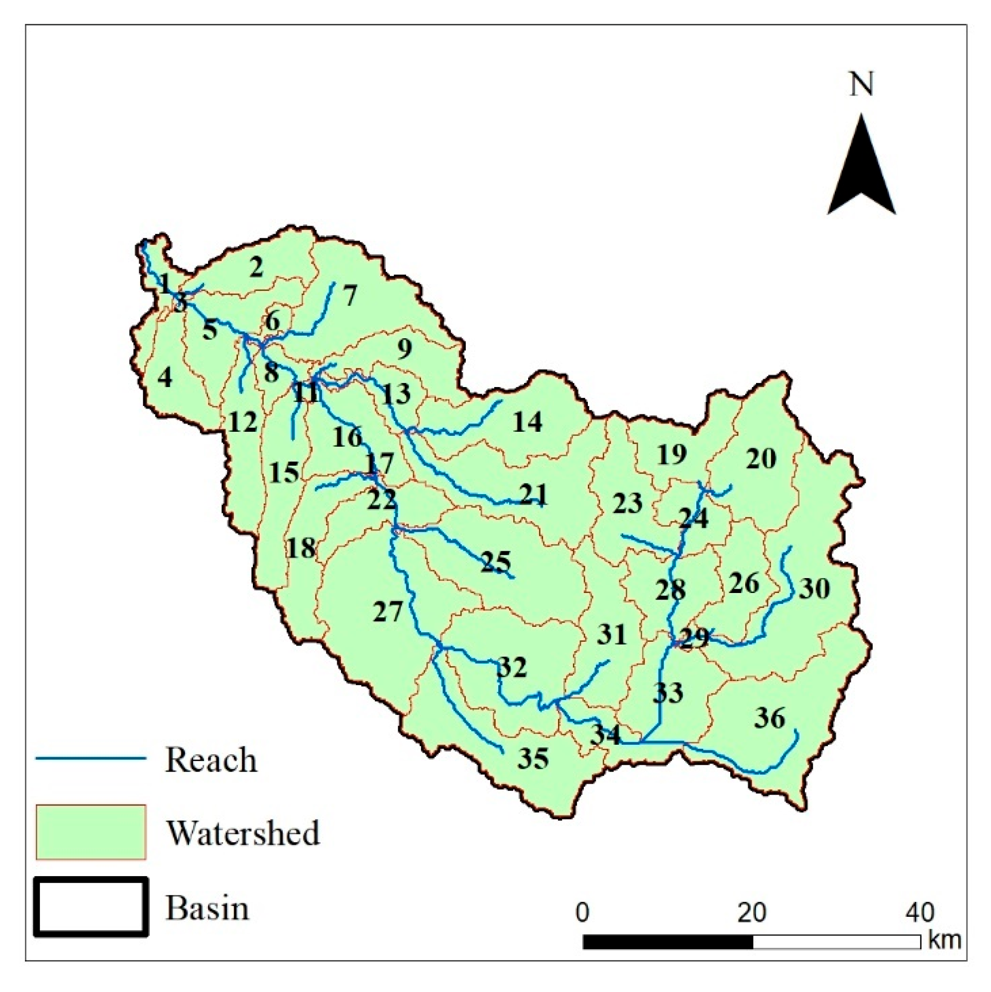
The watershed system was digitized using Google Earth software and extracted using ArcGIS 10.2, and the watershed was divided into 36 sub-basins, as shown in Figure 2.
2.2.2. Types of Land Use
The type of land use has a relatively large impact on the model’s simulation results, and the land use in 2000, 2010, and 2020 were chosen due to the different changes in each period. The study area was uniformly processed to a raster size of 90 × 90 m by cropping it and converting it to GRID format, as shown in Figure 3. In Figure 3, AGRL represents agricultural land, BERM represents grassland, FRST represents forest land, URMD represents urban land, URML represents unused land, and WATR represents water.
2.2.3. Types of Soil Data
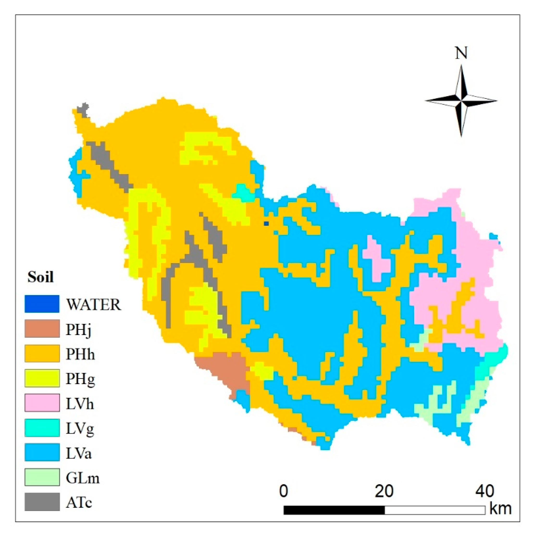
Soil data were obtained from the HWSD China Soil District; more specifically, they were obtained from the 1:1 million soil data provided by the second survey of all Chinese soils in GIRD format. They were then classified by the FAO-90 soil classification system and processed by the soil classification system. Figure 4 depicts the soil type map and Table 2 depicts the soil classification correspondence.
2.2.4. Meteorological Data
2.3. Model Introduction
SWAT is a watershed-scale model for assessing the effects of various land use and management practices on water quantity and quality over time. Weather, hydrology, soil temperature and properties, plant growth, and land management are the main components of the phase model, and all hydrologic processes can be simulated using the water balance equation (Equation (1)) [26].
where is the final soil water content (mm) at time t (days), is the initial soil water content on day (mm), is the precipitation of the -th day (mm), is the surface runoff on day (mm), is the evapotranspiration on day (mm), is the infiltration water at the bottom of the soil on day (mm), and is the amount of water returned to groundwater on day (mm).
Figure 6 describes the whole process of SWAT model operation.
2.4. Validation Criteria and Model Parameter Rates
In this paper, we choose 2 methods—decision coefficient (R2) and Nash–Sutcliffe simulation efficiency coefficient (NS)—as the measure of model efficiency [27].
The coefficient of determination (R2) is calculated as Equation (2).
The Nash–Sutcliffe simulation efficiency factor (NS) is calculated as Equation (3).
Both R2 and NS are simulated and calibrated by SWAT-cup, where Qobs is the measured value, Qsim is the simulated value, and Qavg is the average of all simulated values.
3. Results and Analysis
3.1. Model Practicality Analysis
The relevance of the selected parameters and the values taken are presented in Table 5 by selecting sub-basin 17 as the rate determination of monthly runoff data and sub-basin 1 discharge as the simulation validation of nitrogen and phosphorus, based on the studies of Ahmad and Chen, et al. for reference [28,29].
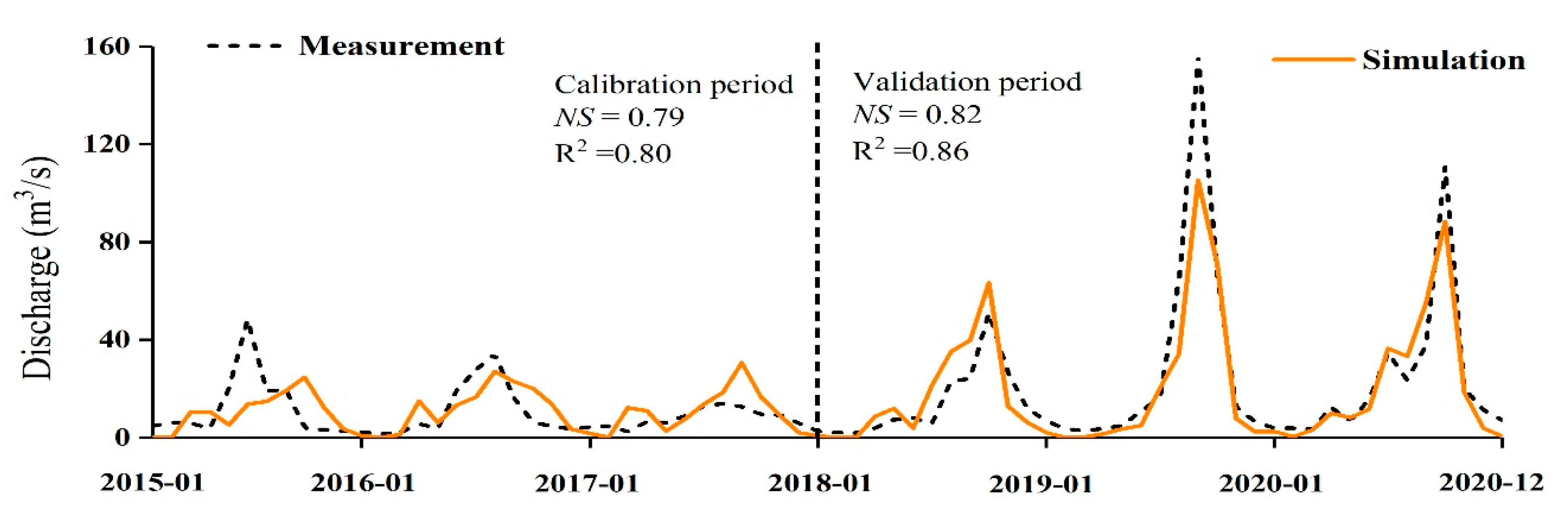
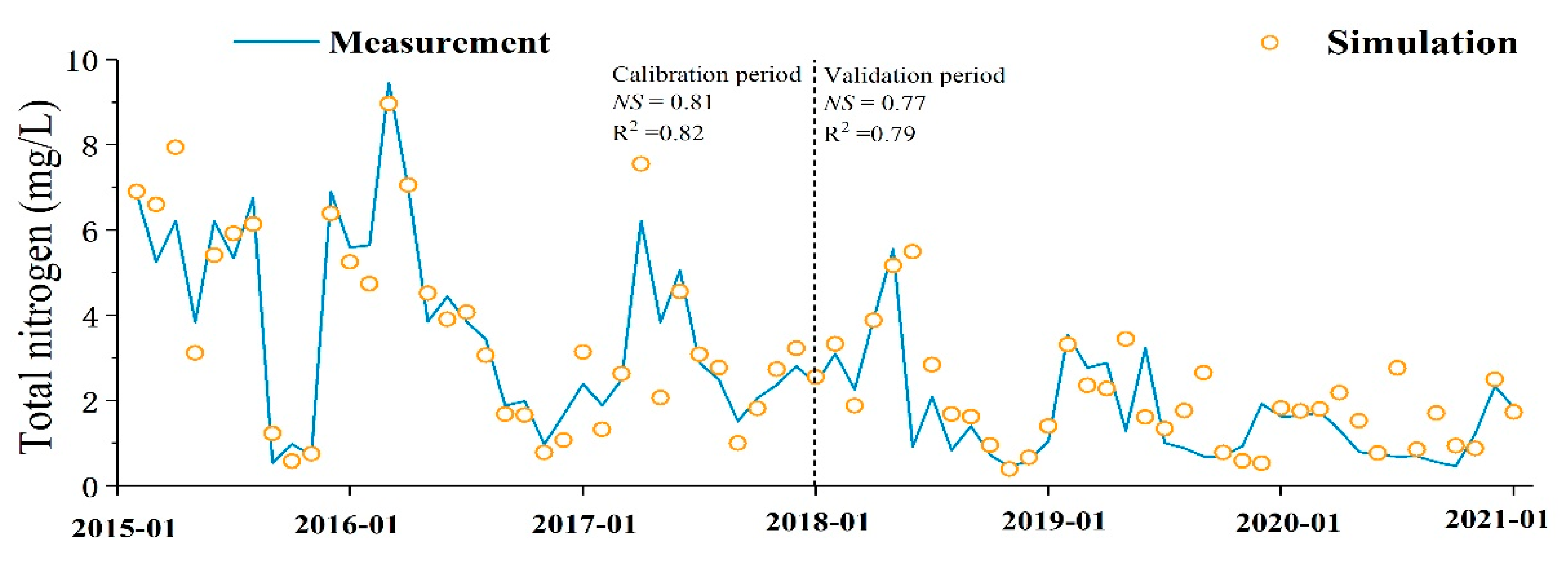
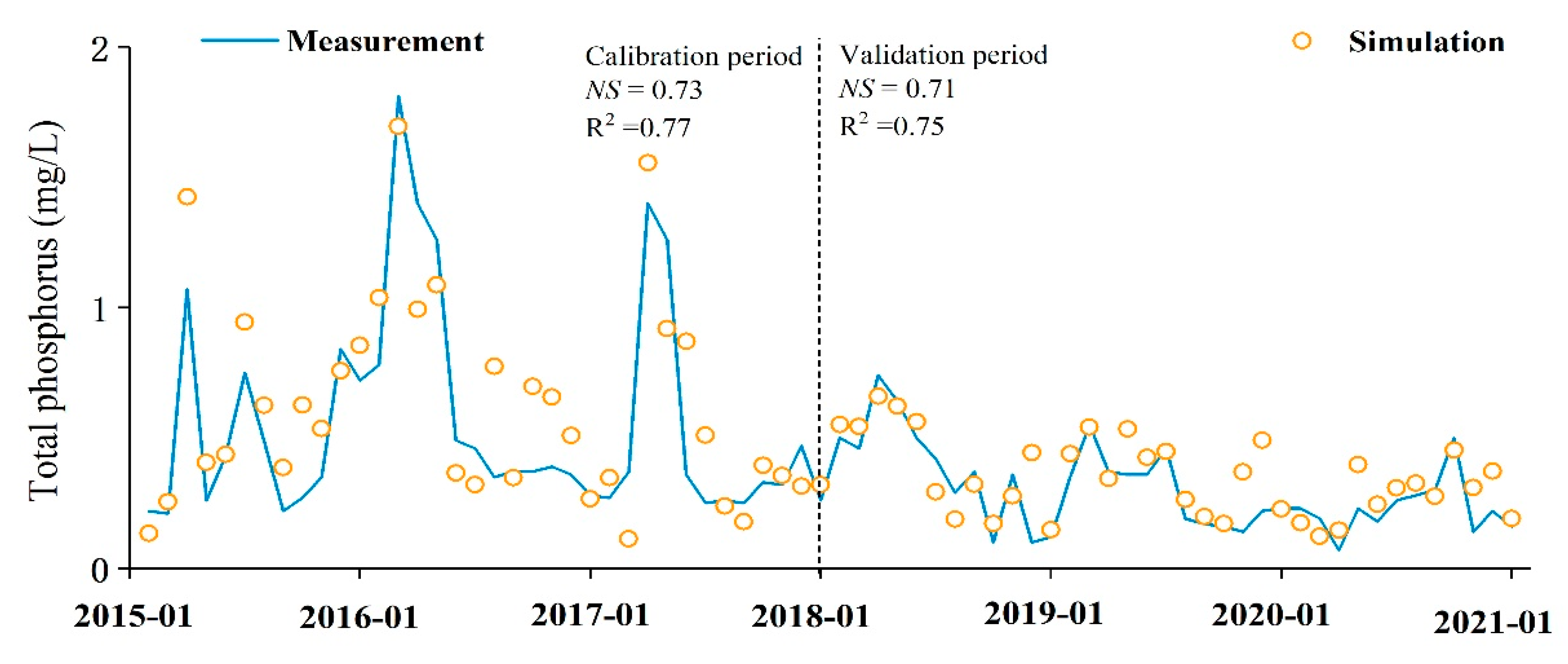
In this research, the model warm-up term is 2012–2014, the rate period is 2015–2017, and the validation term is 2018–2020. Figure 7, Figure 8 and Figure 9 depict the model simulation but also the measured effects.
The effect of monthly simulated runoff is relatively good, as can be seen in Figure 7. The rate period’s NS and R2 are 0.79 and 0.80, respectively, and the validation period’s NS and R2 are 0.82 and 0.86, respectively, while Figure 8 and Figure 9 display the simulation effect of total nitrogen and total phosphorus, which both surpassed 0.75, indicating that the simulation effect is very suitable for the area and can fully describe changes in soil and water pollution in the area, which can be simulated and analyzed in some way.
3.2. Analysis of Quantitative Changes in Land Use in the ARB
3.2.1. Land Use Change
The statistics of land use area of the Ashe River Basin were carried out using ArcGIS software’s statistical categorization for three periods of 2000, 2010, and 2020, and the land use area changes were produced in Table 6.
The main land types in the Ashe River basin are arable land and forest land, as shown in Table 6. In the years 2000, 2010, and 2020, 3234.92 km2 (92.4%), 3227.92 km2 (92.2%), and 3115.89 km2 (89.0%), respectively, are inhabited. The area of arable land, forest land, and grassland has been steadily decreasing according to many types of statistics. The amount of water, urban land, and undeveloped land, on the other hand, is gradually increasing. Arable land shrinks the most, by 27.34 km2 from 2000 to 2010, and by 72.95 km2 from 2010 to 2020, followed by forest land, which grows by 17.89 km2 from 2000 to 2010 but then shrinks by 38.45 km2 from 2010. From 2000 to 2020, grassland declines by 17.02 km2, while the increase or decrease of the water area is the least among the six kinds. From 2000 to 2010, 1.03 km2 decreased, then increased by 2.37 km2 from 2010. Both urban and unused land are expanding, with 92.07 and 44.50 km2 added, respectively. Both land for urban use and unused land are increasing, with 92.07 and 44.50 km2 increases, respectively.
Overall, the decline in arable land, grassland, and forest land is the highest, totaling 100.29 km2; on the other hand, the rise in urban land is the largest, totaling 92.07 km2.
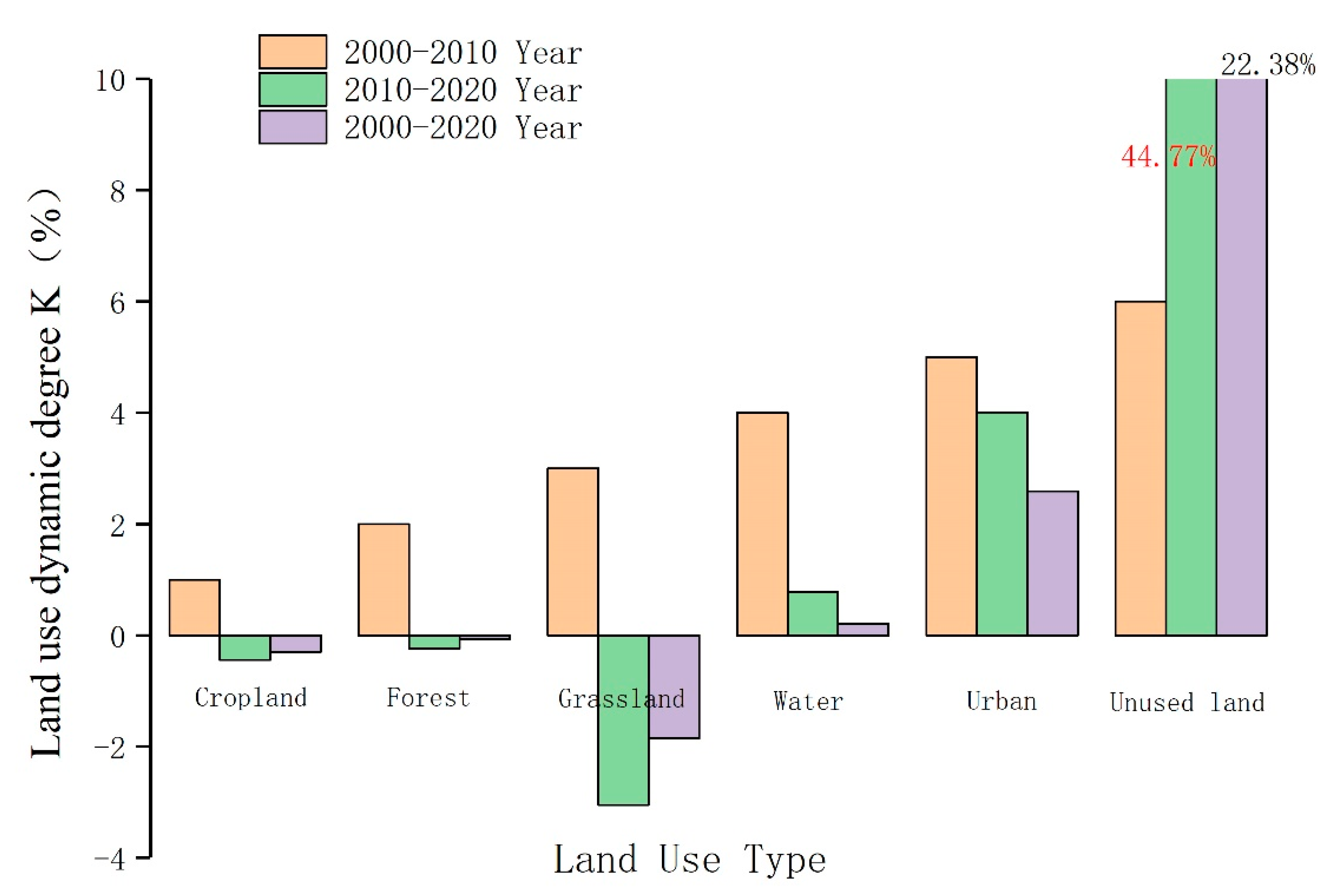
Land use change can also be analyzed using a land use dynamic degree [30], which uses a single land use type to depict the rate of change of that type through time, with the formula written as Equation (4).
where is a particular land use single land use dynamic degree during the study period, is the area of a certain land use/cover type at moment a at the beginning of the study (km2), is the area of a certain land use/cover type at moment b at the beginning of the study (km2), is the length of the study period, and if the unit is year, is the dynamic degree of a certain land use in the study area during the time period.
When > 0, it means that the area of the type is in a gradual growth trend; on the contrary, when < 0, it means that the area of the type is in a decreasing trend. Meanwhile, when = 0, it means that the area of the type in the area has not changed during this period.
Table 6 depicts that arable land and grassland have been declining in recent years, while unused land and urban land have been rising, forest land has been increasing and then reducing, and watershed has been falling and then increasing. The largest increases in the magnitude of land use from the dynamic degree in the period 2000–2010 is in towns, with a coefficient of 0.83%, while the largest reduction is in grasslands, with a coefficient of −0.94%. Cropland and forest land are changing at slower paces of −0.16 and −0.11%, respectively. −0.33% is a moderate rate of change in water area. The state of undeveloped land remained stable. From 2000 to 2020 as a whole, the most significant change, excluding the change in unused land, is in urban land, followed by grassland, with 2.59% and −1.85%, respectively. The gradual growth of urban land is closely related to the economic development within the ARB. From 2000 to 2020 as a whole, the most significant change, excluding the change in unused land, is in urban land, followed by grassland, with 2.59% and −1.85%, respectively. The gradual growth of urban land is closely related to the economic development within the ARB. The dynamic degree of land use is shown in Figure 10, which is presented by means of markers because 44.77% of unused land varies too much from 22.38% and other values.
3.2.2. Land Use Transfer Matrix
From the analysis of changes in land use quantities as well as dynamic degrees, only a single change of situation can be known. However, the total area of the watershed constant, as well as the matrix transfer table, can be evaluated by changes in land use types through time. The land use matrix can reflect dynamic information on the change of various land types over time and can be studied by the area transferred into and out of a certain land area over time [31].
The matrix expression is Equation (5).
where is the area of the land use type in the i-th land use type conversion , indicates the total number of land use types.
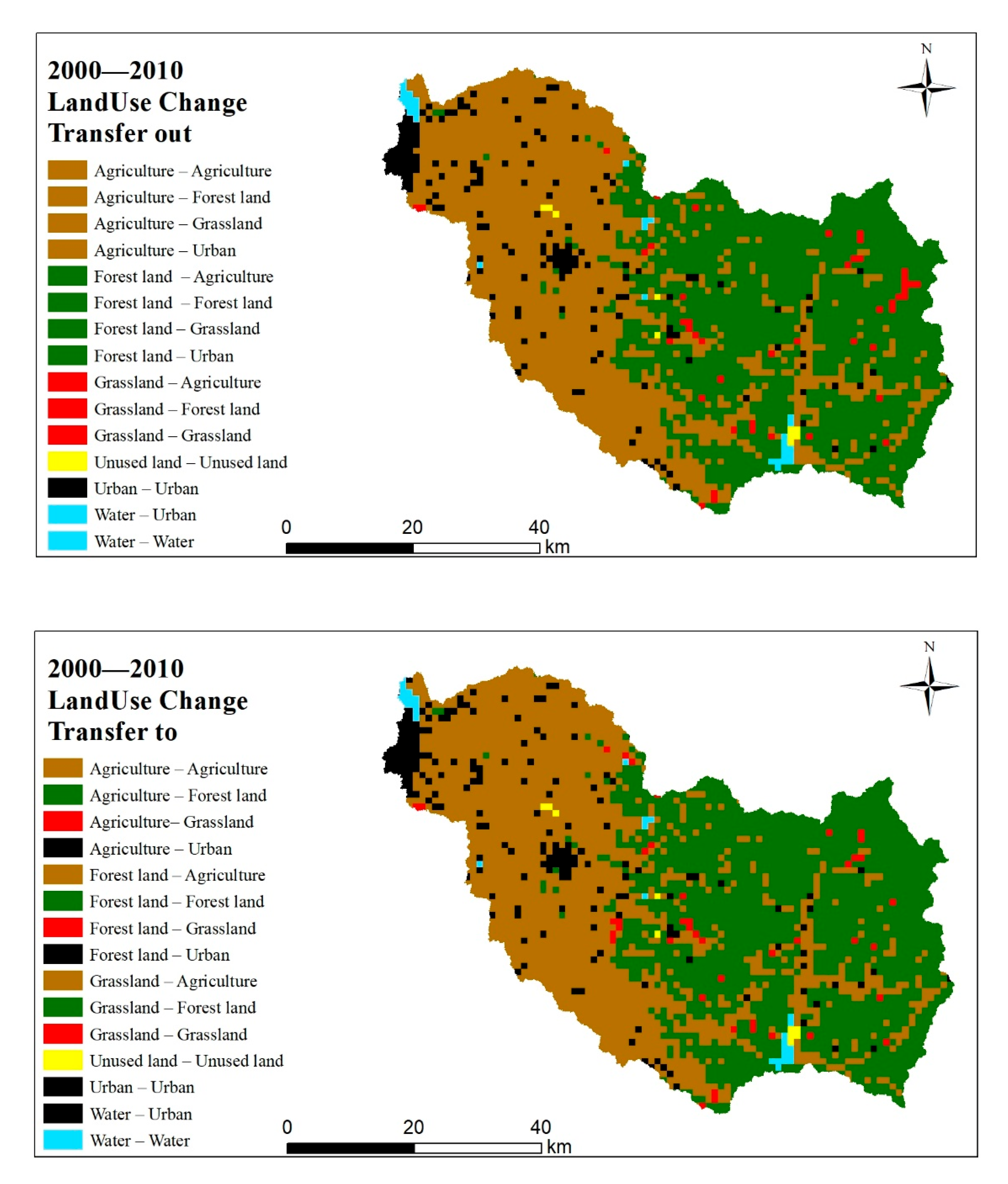
According to Table 7, the transfer out in 2000 was as follows: initially, the majority of the arable land was transferred out to urban and forest land, with just a tiny portion transferred out to grassland. The total area transported out was 12.73, 10.91, and 5.78 km2. The area of forest land transferred to cropland, grassland, and urban land is 1.04 km2; grassland is mostly transferred to forest land, with an area of 10.10 km2 accounting for 22% of grassland area; and there is essentially no change in water, urban land, and unused land. The area of arable land transferred to forest land and grassland is equal but tiny at 1.01 km2; forest land was transferred from arable land and grassland to 10.91 and 10.10 km2 correspondingly, and grassland was transferred to 5.78 km2 of arable land area and 1.04 km2 of forest land area. Through arable land, forest land, and water area, urban land was shifted to 12.73, 1.04, and 1.04 km2, respectively. Taken as a whole, the land use transition from 2000 to 2010 was minimal since development was still in its early stages. The most arable land, forest land, and grassland were transferred out, with 29.43, 3.12, and 11.15 km2 transferred out, respectively.
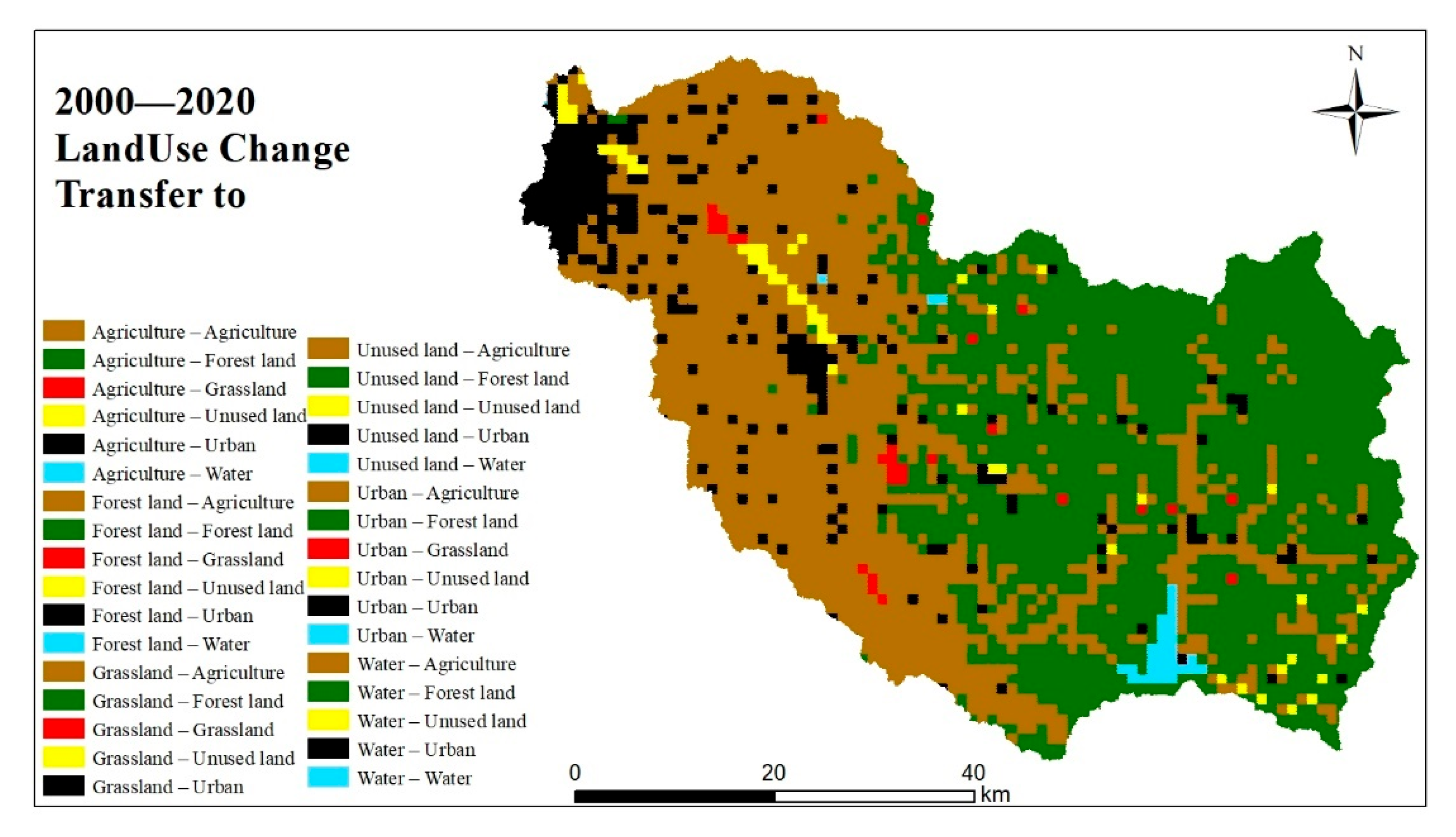
There are two diagrams in Figure 11, representing the transfer out and transfer in of land use. We can see the same color of each transfer out by the transfer out graph, while in the bottom one we can compare well that the transfer out part is transformed into a different land use. For example, in the middle part of the unused land represented in red, some of it turns into yellow for cropland and some of it turns into green for forest land. (Figure 11).
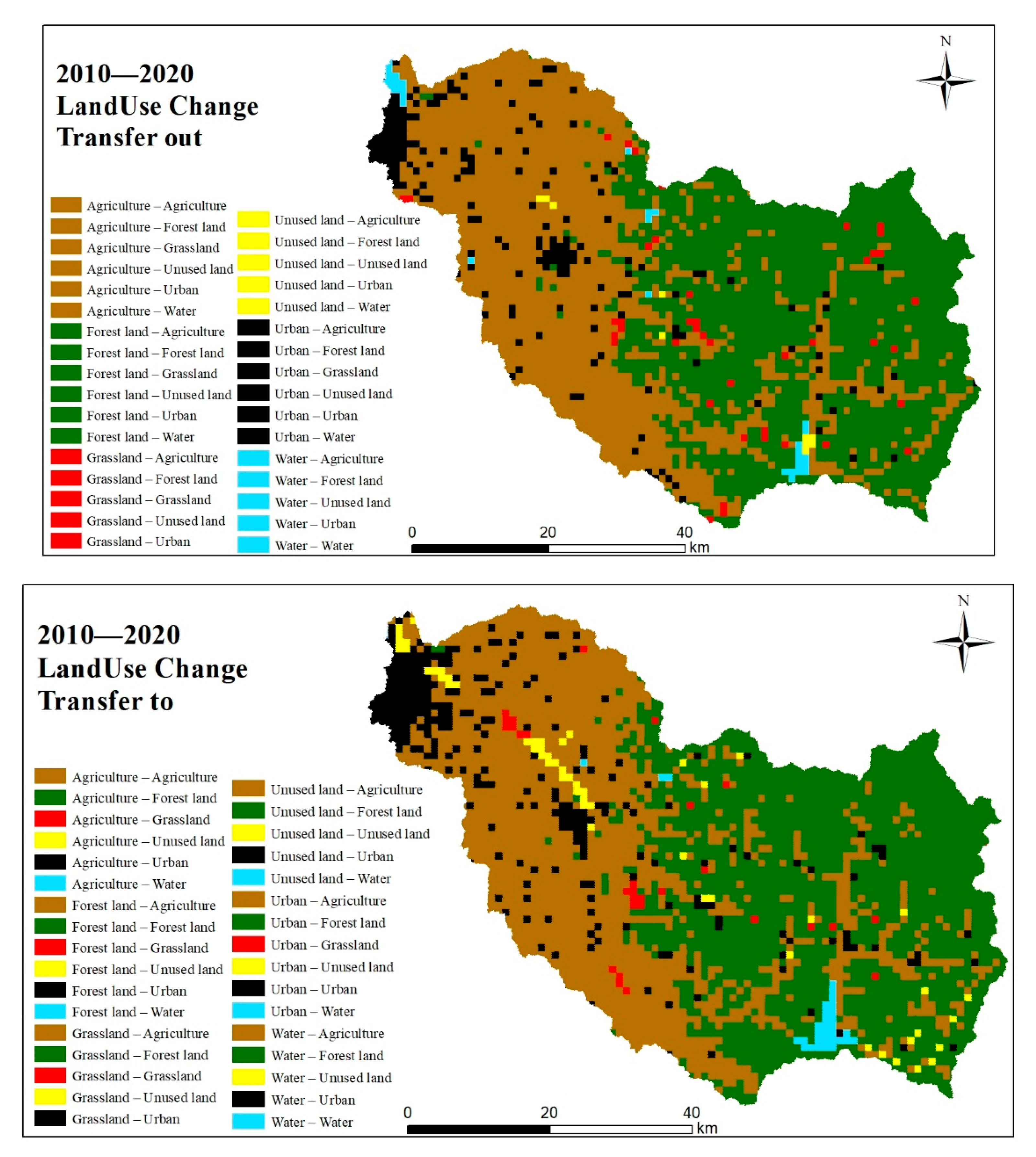
According to Table 8, between 2010 and 2020, arable land was predominantly turned into forest land and towns, totaling 188.19 and 161.90 km2, respectively, with a tiny part converted into grassland, water, and unused land. The transfer of forest land was primarily to cropland, with an area of 221.86 km2 accounting for 14% of forest land. A small portion of urban land was turned into arable land, but as far as the 2010 transfer out is concerned, urban land increased by 161.90 km2, which indicates that it is tending to be urbanized. 12.60 km2 of grassland was transferred to cropland and 23.93 km2 to forest land, accounting for 30 and 57% of grassland, respectively. The area transferred out of waters is smaller, but even the area transferred between unused land to waters is larger, accounting for more than half of the total. Concerning the 2020 transfer in, first and foremost, agricultural transfer in was mostly by forest land and urban land, with areas of 221.86 and 94.57 km2, respectively. The area shifted from agriculture to forest land totals 188.19 km2. In comparison to 2010, the area transferred from grassland to forest land totals 188.19 km2. In comparison to 2010, the transfer of grassland is around 10 km2 less than the transfer out; the major difference is the transfer of cropland, which reaches 161.90 km2 and will reach 269.87 km2 in 2020 (Figure 12).
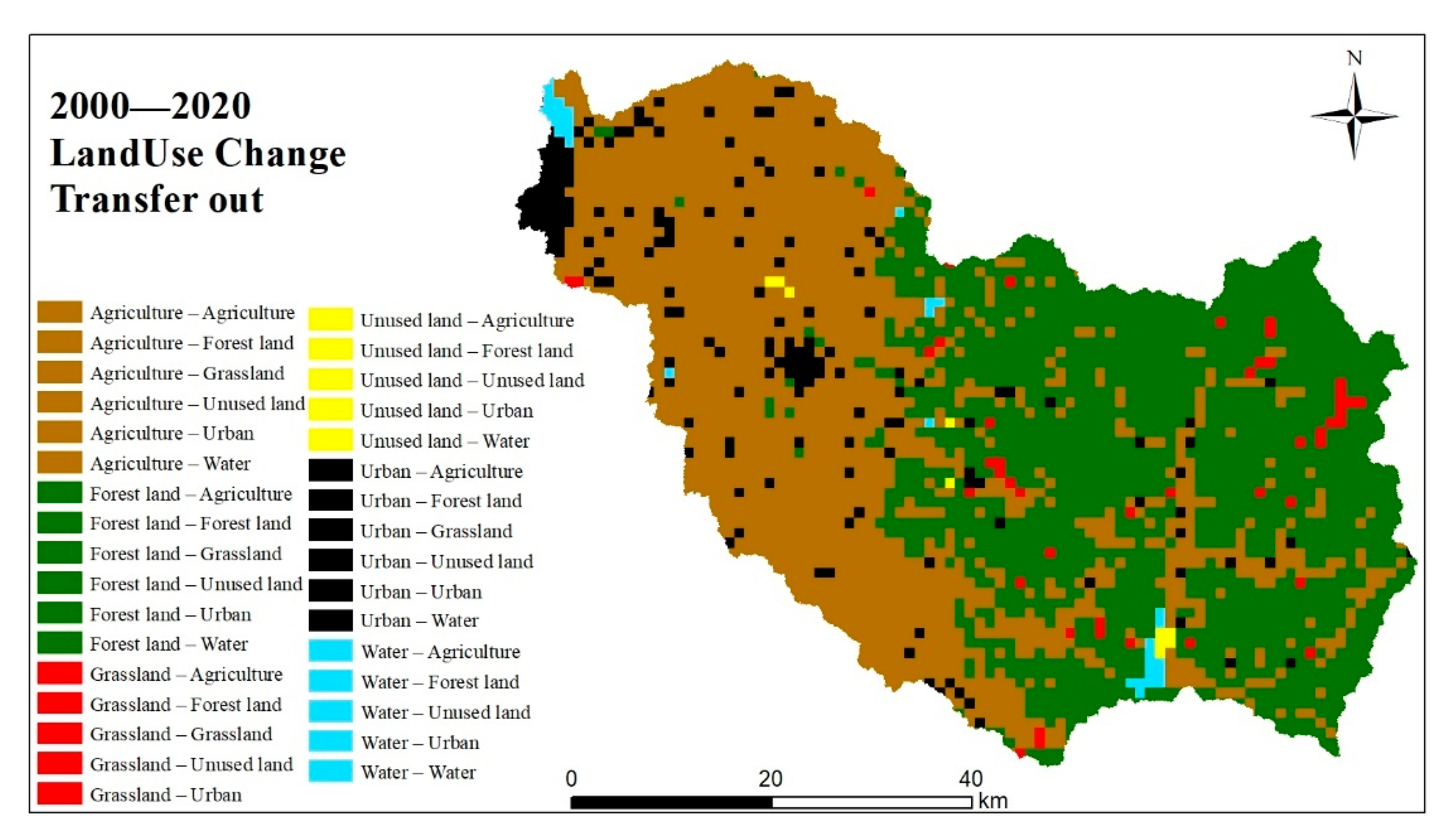
The land use changes were analyzed using the aforementioned tabular observations of the two time periods. Table 9 shows the entire land use transfer matrix analysis for 2000–2020 to better examine the changes in land use area in the ARB.
Looking at the land use types in the ARB over the last twenty-one years, 191.07 km2 of arable land transferred since 2000 has been transferred to forest land, while 171.82 km2 has been transferred to urban land. Forest land has primarily been transferred to arable land, with an area of 217.01 km2. Watershed is transferred into forest land, townland, and unused land, with areas of 6.32, 6.27, and 5.19 km2, respectively. Townland is mostly transferred out of arable land (90.97 km2), and unused land is mainly transferred out of watershed, with an area of 5.02 km2.
According to the transfer situation in 2020, arable land is primarily transferred through forest land and urban land, with areas of 217.01 and 90.97 km2, respectively. Forest land is primarily transferred through arable land and grassland, with areas of 191.07 and 33.29 km2, respectively.
Grassland is transferred from cropland and forest land, which provide areas of 15.36 and 10.24 km2, respectively. Water is transferred principally through 13.30 km2 of cropland, and urban land is transferred predominantly through cropland and forest land, which have areas of 171.82 and 19.77 km2, respectively. The percentage of unused land has increased from 9.94 in 2000 to 54.44 in 2020, owing primarily to population growth. The amount of unused land increased from 9.94 km2 in 2000 to 54.44 km2 in 2020, owing mostly to the transfer of 28.65 km2 of arable land and 14.77 km2 of forest land.
In summary, the mainland types transferred out are arable land and forest land, with 451.89 km2 and 296.69 km2 transferred out, respectively. Even though the area transferred out of grassland is just 46.03 km2, the proportion of transferred out area is 99.9%. Cultivated land is the primary source of transfer to other types of land (Figure 13).
3.3. Runoff Changes under Different Land Use Scenarios
3.3.1. Analysis of Simulation Results at the Annual Scale
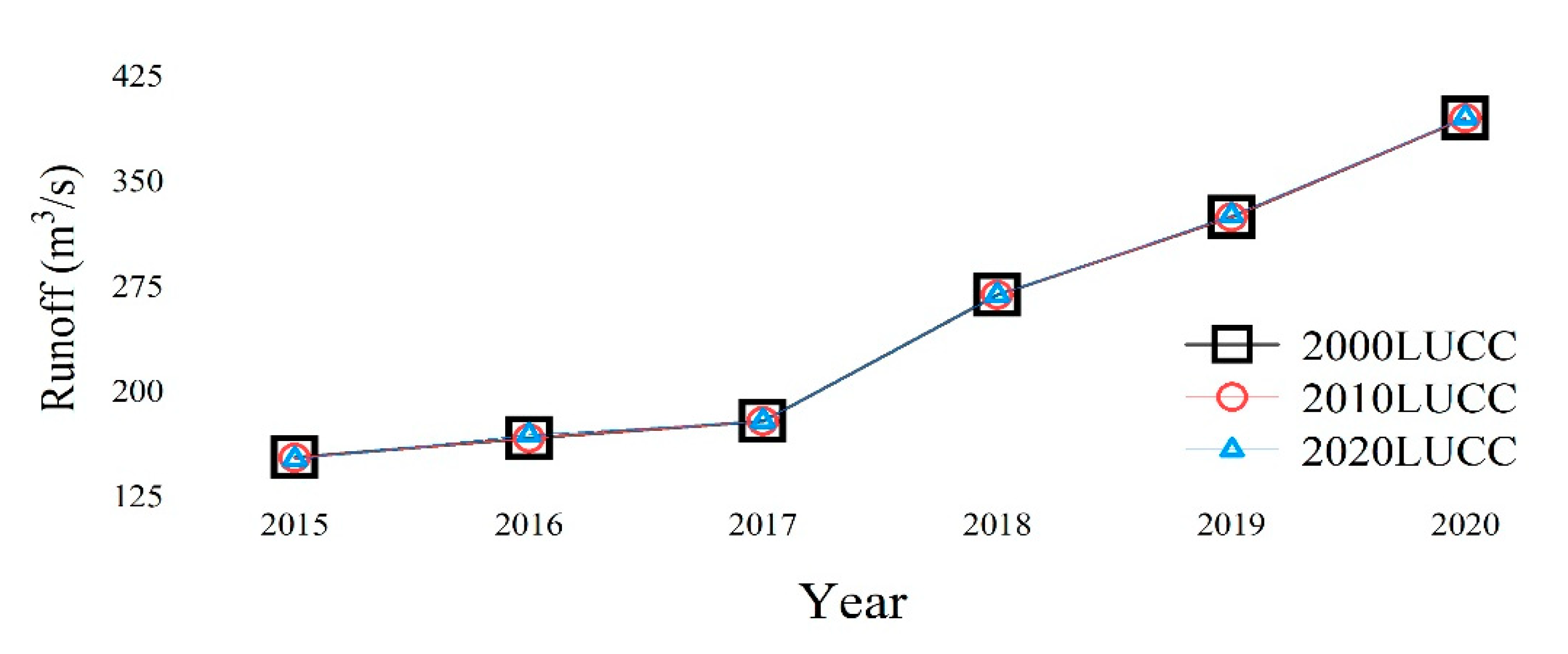
The runoff data selected for the period from 2015 to 2020 are considered the observations for rate determination and validation in this paper. The land use in 2020 is loaded into the SWAT model, and the yearly variation of runoff is produced by examining the monthly scale and then the land use maps of 2000, 2010, and 2020, and reducing calculation error by holding the other values and thresholds constant (Figure 14).
The figure indicates that the value of yearly runoff increases year after year, but the land use map of the three phases has little or no effect on the change of runoff. The land use in the study area has no substantial impact on runoff.
3.3.2. Analysis of Simulation Results at the Monthly Scale
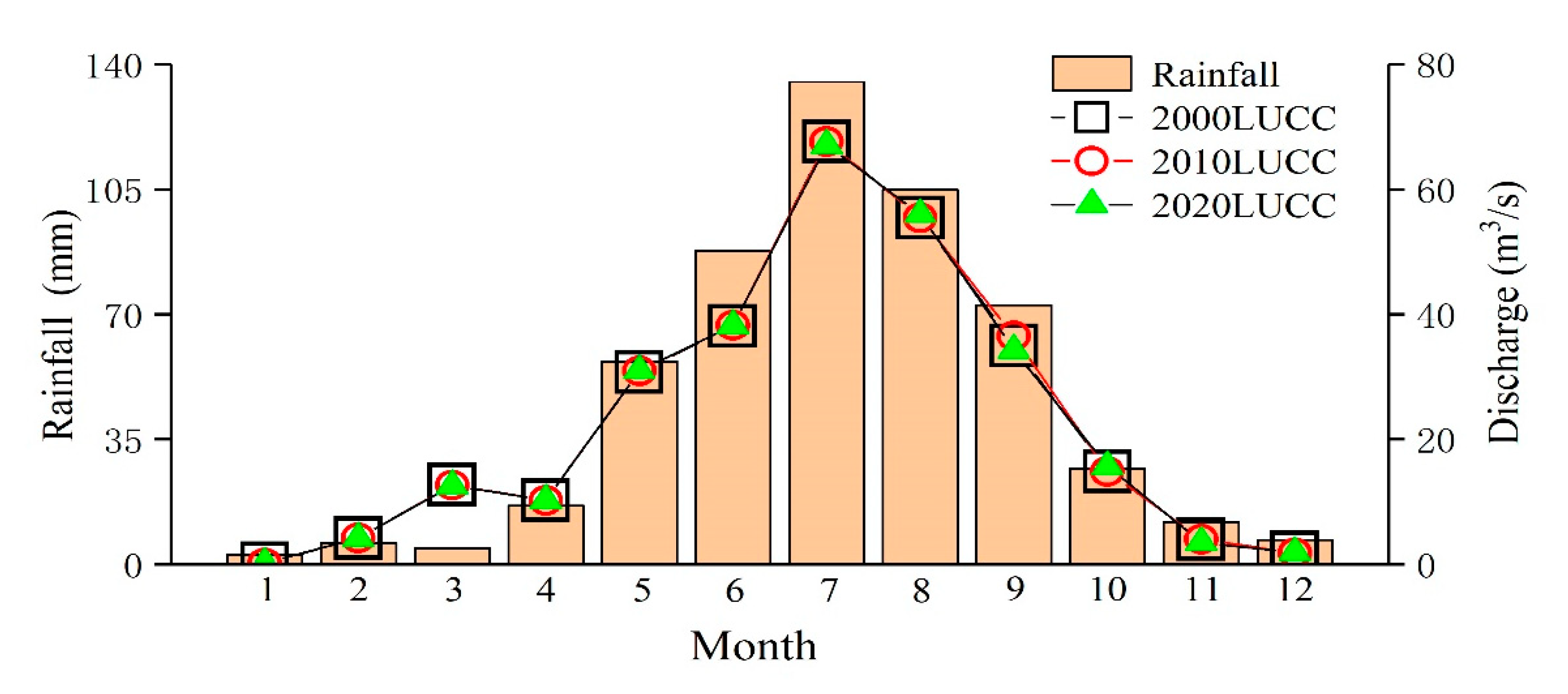
The monthly runoff simulation differs from the annual simulation in that the monthly runoff varies positively with rainfall. The changes in land use and annual runoff are constant and do not range much across the three time periods (Figure 15).
On a monthly scale, the runoff volume reveals an increasing and subsequently decreasing tendency. The runoff volume from May to September is higher, accounting for 81% of the total annual runoff volume, and the runoff volume in the other months is low, which is related to the Ashe River’s weather, with less rain in spring and winter and more rain in summer, i.e., from June to September, than the rest of the year, so the net flow is also higher. The volume of runoff is modest from January to April, begins to increase in May, and progressively decreases after reaching a peak in July.
During the modeled years, the multi-year average monthly runoff in the Ashe River basin is 275.5 m3/s, with the average monthly runoff in 2010 being 0.29 m3/s higher than in 2000 and 0.57 m3/s higher in 2020 than in 2010, indicating that runoff is not strongly related to land use changes, but rather to weather changes such as precipitation, evaporation, and seepage.
3.4. Changes in Total Nitrogen under Different Land Use Scenarios
3.4.1. Simulation Analysis of Total Nitrogen at Annual Scale
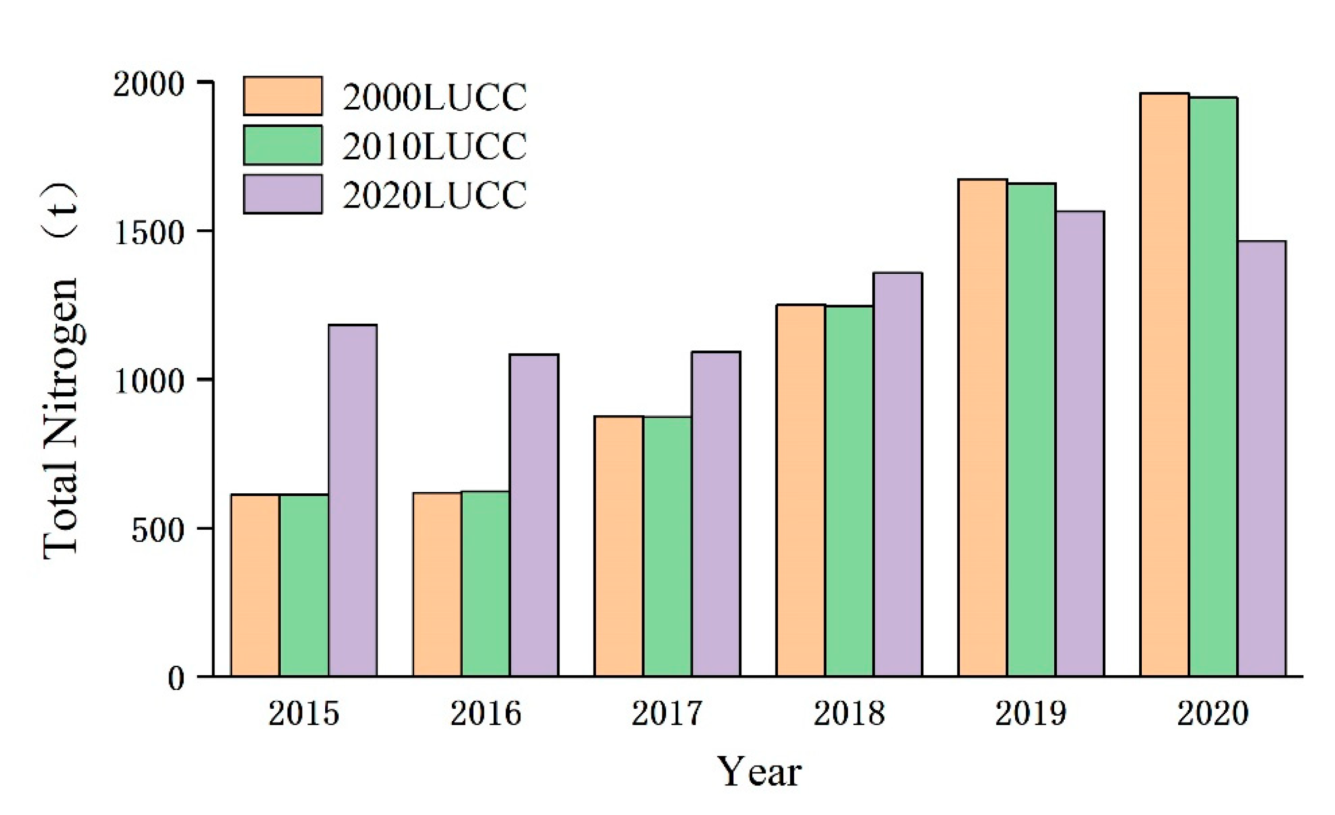
The research was carried out on an annual scale using land use data from three separate periods (Figure 16). The nitrogen loads exported from the basin show a heterogeneous pattern of nitrogen changes from 2015 to 2020. The land use map load for 2020, for example, where the highest load was achieved in 2020 with a value of 1962.39 t. The lowest value was achieved in 2015, with a value of 611.63 t. In the period 2015–2020, the average yearly total nitrogen load was 7234.12 t.
When the total nitrogen load is examined over three different periods, it is clear that the trajectory of load changes differs; the load in 2000 and 2010 increases, whereas the total nitrogen load in 2020 first declines and then grows in the state, from 611.62 t in 2000 to 1182.03 t in 2010. It is clear here that the influence of increased urbanization on nitrogen begins to grow steadily larger. The changes in 2015, 2016, and 2017 are visible in the three land use differences, but the changes in 2018, 2019, and 2020 begin to diminish progressively.
3.4.2. Simulation Analysis of Total Nitrogen at Monthly Scales
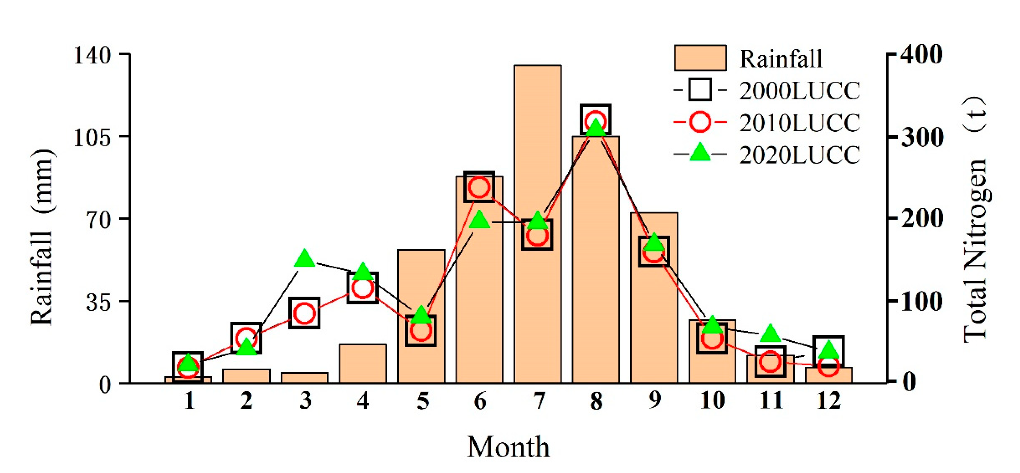
The simulated process at the monthly scale has an increasing and subsequently declining tendency, with the total nitrogen export in the research area being evaluated. This figure demonstrates that the total nitrogen load has a clear peak in months 6 and 8, and for the land usage in 2020, for example, total nitrogen hits 185.94 t in June and then begins to fall until it reaches 302.80 t in August. The rainfall in the research area is mostly focused on May to September, with only a minor fluctuation in the total nitrogen load (Figure 17).
Overall, by studying land use in each of the three eras, it is discovered that the change in total nitrogen also varies very little due to the small variation in land use change between 2000 and 2010. In contrast, the land use change in 2020 is more visible, and it can be seen that as towns grow, woodlands and grasslands shrink. As towns grow and woodlands and grasslands shrink, the nitrogen content grows. The monthly average total nitrogen load gradually climbed from 96.71 t in 2000 to 98.68 t in 2010, and eventually to 107.59 t in 2020.
3.4.3. Spatial Distribution Characteristics of Total Nitrogen
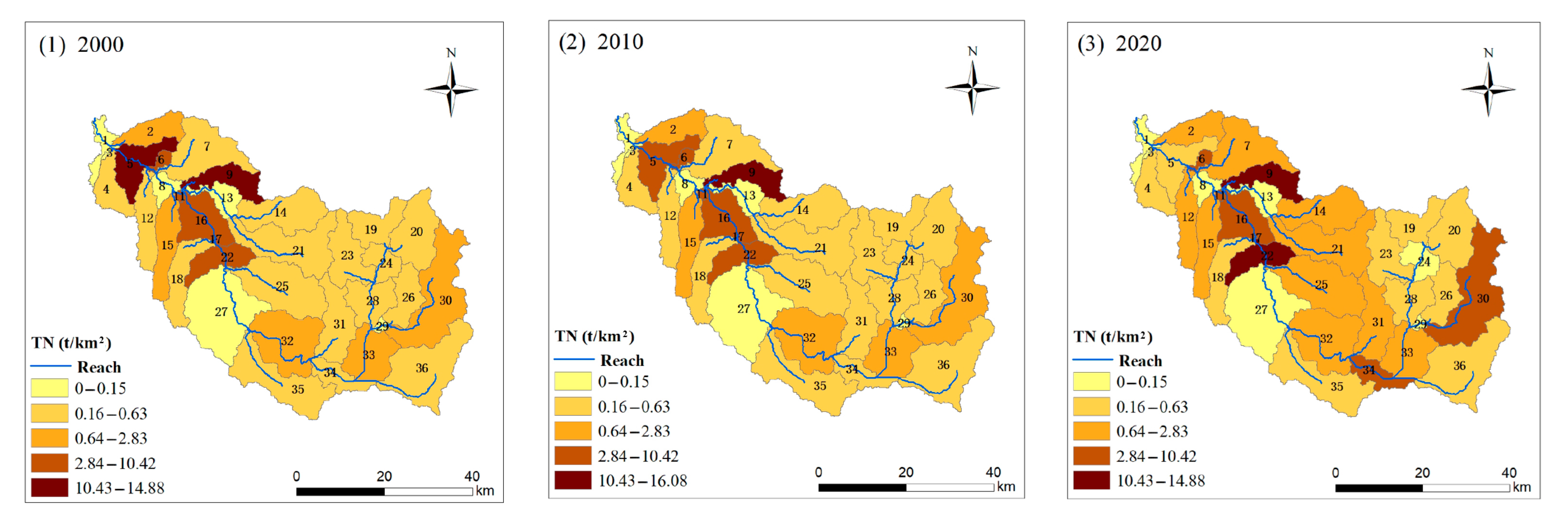
The three land use maps were fed into the SWAT model, which calculated the average annual load per unit for each sub-basin in 2000, 2010, and 2020 (Figure 18). From here on, everything written is the simulated value from the software simulation, not the actual measured value.
According to the estimate, the average annual load of total nitrogen per unit area usually increased, rising from 2.40 t/km2 in 2000 to 2.74 t/km2 in 2010 and 2.78 t/km2 in 2020. The average yearly load of total nitrogen per unit in all sub-basins in 2000 may be observed from the geographical distribution, which is normally in the range of 0–16.19 t/km2.
The more serious pollution is in the main stream’s downstream section, and the average annual unit load of each sub-basin, namely 5, 6, 9, 11, 16, 17, and 22, is more than 2.83 t/km2, with sub-basins 5 and 9 reaching more than 10, 10.42 and 13.47 t/km2, respectively. Because of the smaller area of the two sub-basins and the bigger average yearly total nitrogen load pooled, the total nitrogen per unit area of the watershed is relatively high.
The total nitrogen load per unit in 2010 is typically more balanced than in 2000, owing to minor land use changes and the presence of larger loads in main streams and downstream of watersheds. For the more heavily loaded watersheds 5, 6, 9, 11, 16, 17, and 22, 2010 remains the same as 2000. The total load per unit area has dropped; however, the difference is not especially substantial.
The total nitrogen load per unit in 2020 is more varied than in 2000, but it is also concentrated in the watersheds of the main streams, where seven sub-basins, namely 6, 9, 11, 16, 17, 22, 34, and 30, surpass 2.83 t/km2. 34 and 30, respectively, greater than in 2000, whereas sub-basin 5 is reduced. Sub-basins 9 and 22 were the most contaminated, with 14.89 and 12.83 t/km2, respectively. This is linked to changes in land use, human activity, and geography. Land use changes in the Ashe River basin can be recognized as the key factor in this study based on modeling results.
3.5. Changes in Total Phosphorus under Different Land Use Scenarios
3.5.1. Simulation Analysis of Total Phosphorus at Annual Scale
SWAT model rate determination was used to analyze changes in total phosphorus loadings in the Ashe River basin over three time periods and then integrated into land use maps for 2000, 2010, and 2020 (Figure 19).
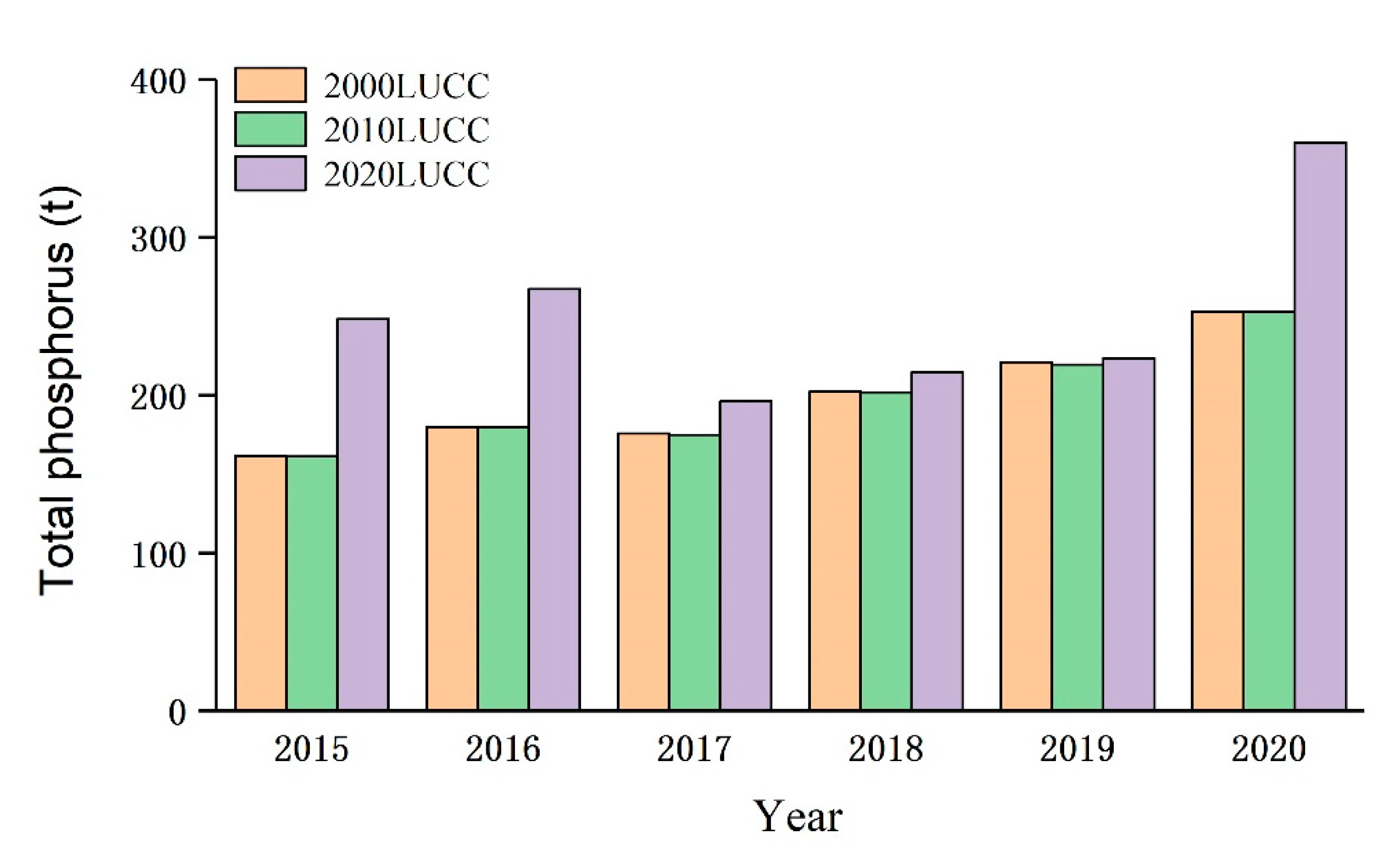
For example, the average annual load of total phosphorus was 251.3 t in the period of 2020, reaching a maximum of 360 t in 2020, followed by 2016 and 2015. The changes in the total phosphorus load in three different periods were not very different, but both had a trend of increasing year by year, with the average annual load in the 2000 period being 198.82 t and reaching 201.21 t in the 2010 period, whereas the load in the 2020 period gradually increased from 248.1 to 267.18 t in 2015, and then gradually decreased to 248.1 t in 2016. The load in the 2020 era climbed progressively from 248.1 to 267.18 t in 2015, then decreased for three years before reaching its maximum amount of 360 t in 2020.
3.5.2. Simulation Analysis of Total Phosphorus at Monthly Scales
By examining the pollutant load of total exported total phosphorus in the study area, the monthly scale simulations were similar to the annual scale simulations (Figure 20).
The variations in monthly rainfall and monthly total phosphorus load are consistent, according to the graph, and the correlation coefficient reached 0.86 by looking at the land use map for the year 2020, showing that the two are positively associated. The total nitrogen load created with little change in land use was similar in 2000 and 2010, showing that the total nitrogen load generated with little change in land use is similar. Additionally, in the 2020 period, land use followed the same pattern as the previous two, but with a shift in value. The value of total phosphorus gradually increased with the rise in rainfall from June to September, peaking at 58.91 t in September.
In general, as rainfall increases from June to September, a huge number of pollutants seep into rivers, lakes, and seas via precipitation, and as rainfall declines with the winter, so do the contaminants. The monthly average total phosphorus load climbed significantly from 16.63 t in 2000 to 16.80 t in 2010, and then to 20.97 t in 2020.
3.5.3. Spatial Distribution Characteristics of Total Phosphorus
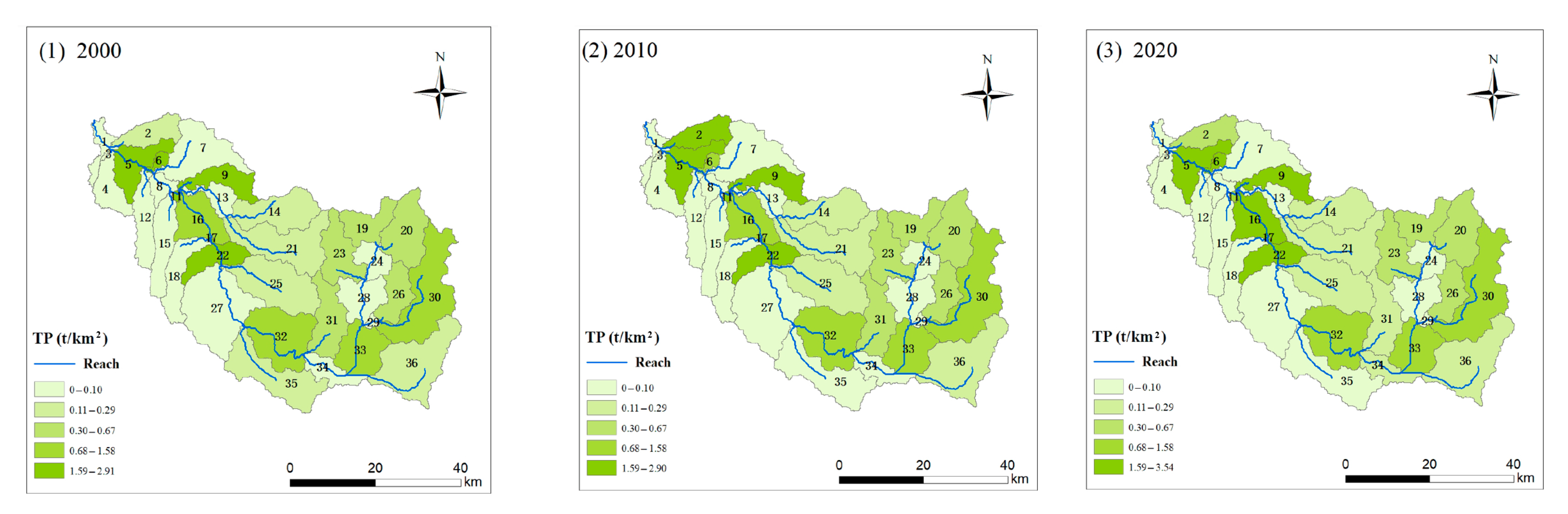
The average annual change in total phosphorus units for individual sub-basins of the three phases in 2000, 2010, and 2020 was studied based on simulation results obtained by inputting land use into the SWAT model for different periods of the three phases (Figure 21).
The average annual total phosphorus load per unit obtained from the three stages follows the same pattern as the average annual total phosphorus, increasing from 0.58 t/km2 in 2000 to 0.60 t/km2 in 2010, then gradually increasing to 0.65 t/km2 in 2020. The more significant pollution zones are downstream of the mainstream at the more serious pollution sub-basins 5, 6, 9, 11, 17, and 22, a total of six sub-basins, with annual average total phosphorus loads in the range of 0–2.91 t/km2. Sub-basins 9 and 17 have 2.91 and 2.43 tons per square kilometer, respectively. Sub-basin 17 exceeds 1.58 t/km2 due to its urban location and small area, as does sub-basin 9. The bigger load in sub-basins 5, 6, 9, 11, 17, and 22, a total of 6 sub-basins, all above 1.58 t/km2, with sub-basin 9 still having the greatest load at 2.90 t/km2, a drop of 0.01 t/km2 compared to 2000. A few sub-basins have seen an increase in unit load, for example, sub-basin 2 has grown to 0.29 t/km2.
In 2020, the total unit phosphorus load will remain unchanged from 2010, with six sub-basins above 1.58 t/km2. The average annual total unit phosphorus load has grown in all sub-basins, with a particularly significant increase in sub-basin 9 to 3.5 t/km2 and values in all other sub-basins increasing by more than 15%, with sub-basin 9 increasing by more than 0%.
4. Discussion
We used the SWAT model to replicate the ASR area and discovered that it was able to adapt well to the environment. The water quality and hydrological conditions are as they should be. The only downside is that sediment exploration is not possible. The watershed is not monitored for sediment, and sediment data are not available because of the low sediment content in the area. Although some insensitive data were removed, the model may be better assessed if all of the data can be studied in some way.
The ASR does not alter greatly between the 2000 and 2010 periods for the three different periods of land use, but the decline in arable land and increase in urban land use compared to 2020 suggests that the population is expanding, which may contribute to an increase in urban waste and water pollution. Due to the restricted land use data, we have decided to investigate every decade in this article; however, if we can perform a study every year, we will be able to further explore the consequence of land use change in each year, and whether it moves from quantity to quality. In the future, this could be a more interesting research topic.
This study intended to analyze the analysis of diverse data under various land uses in order to investigate the topic of land use. Because the ASR is located in Harbin’s urban region, its runoff volume is affected by rainfall. Harbin receives 532 mm of annual rainfall on average, with the rainy season lasting from June to September and the runoff amount steadily rising with the rainfall. However, when comparing land use across three years, we discovered that the monthly runoff amount did not change significantly. The volume of runoff has a linear relationship with rainfall—which varies with precipitation, evaporation, and seepage—rather than a direct link with land usage.
Previous research has looked into the impact of various land uses on runoff, but there have been few studies on face-source pollution, particularly in northeastern China. As a result, while this paper uses the SWAT model, it examines not only runoff but also face-source features, and we expect that it will be useful in future research.
On one hand, total nitrogen and total phosphorus both reached their maximum in 2020, as evidenced by the time change in pollution load. The reason for this is the growth of towns and cities, which has resulted in urban waste which has not been treated in a timely manner and has been discharged into the water, causing pollution. On the other hand, the spatial variation of pollution load shows that the pollution in the main stream of the watershed is more serious than that in other sub-basins, partly because sub-basin 1 is the downstream export part and the pollutants generated in the upper watershed are collected in the main stream of the watershed and flow to the outlet to be discharged; this is partly because the main stream is an area with a relatively large area of arable land and when the fertilizer application increases or the fertility of fertilizer application increases, it will cause the overall pollution load to increase.
The difference between nitrogen and phosphorus is that they differ in terms of the value of the annual load; first of all, nitrogen is high throughout the year and develops in a gradual upward trend, reaching a maximum especially in the year 2020. While phosphorus belongs more moderately to the 2000 period and 2010 period, the total phosphorus content is more average; however, in the 2020 period, the phosphorus content increases, then decreases and increases, which is the biggest difference between the two.
The parts shown in the article are data derived from simulations performed by the SWAT model and are not measured values. In China, for example, in the North Ru River area, we can see that the unit load of total nitrogen is between 0 and 3.20 t/km2, while total phosphorus is between 0 and 0.98 t/km2. In the Fu River basin, the unit load of total nitrogen is between 0 and 10.35 t/km2, while total phosphorus is between 0 and 3.15 t/km2. In the Danjiangkou reservoir, the unit load of total nitrogen is 13.35–24 t/km2 and total phosphorus is 5.9–15.0 t/km2, while the model developed in this paper is between 0–16.08 t/km2 for total nitrogen and 0–3.54 t/km2 for total phosphorus. Since different elevations, different climates, and different soil type conditions in each area can cause huge changes, this study looked for areas, some larger and some smaller than the Ashe; while the soils and meteorology do vary, this is unavoidable, but the study’s values are still within a reasonable range. This indicates that the study’s model meets the expected effect and falls in a moderate pollution range when compared to other similar areas [32,33,34].
As a consequence of the simulation findings, it is discovered that ASR contamination grows with the growth of settlements and people. Special sewage treatment plants should be strategically located and created to prevent pollution in the watershed by promoting environmental protection vigorously.
It should be noted that, for starters, we can only study the reservoir and other statistics on pollution discharge using the information now available, and we hope that future workers will be able to acquire better data for better modeling. Second, we are unable to get high-precision remote sensing maps; nevertheless, we expect that these maps will be made available in the future for better analysis. Finally, the pollutant source analysis model may be improved in order to better understand the ecosystem on which humans rely.
5. Conclusions
The SWAT model was used to analyze the simulation results of hydrological and water quality processes in the Ashe River basin; the R2 and NS of runoff simulation for both the rate and validation periods were above 0.79, and the simulation results of TP and TN were also very good, with R2 and NS above 0.75, indicating that the SWAT model has good applicability in the Ashe River basin.
The differences between 2000 and 2010 were not significant, but they were very different from 2020, and the changes in land use in the study area led to different changes in runoff, total nitrogen, and total phosphorus, with the changes in runoff having no significant effect with the differences in land use. The time influence of total nitrogen and total phosphorus is growing, while their geographical distribution is becoming more constant. The most contaminated regions are centered along the mainstem in the middle and lower portions of the basin, and the load per unit area of most of the basin has been increasing since 2000, with a few exceptions.
This article can serve as a foundation and reference for the watershed’s pollution management and environmental preservation.
Author Contributions
Conceptualization, C.D.; methodology, C.D. and J.C.; software, J.C. and S.T.; validation, T.N. and X.H.; writing—original draft, J.C.; writing—review and editing, T.N. and J.C.; funding acquisition, C.D. and T.N. All authors have read and agreed to the published version of the manuscript.
Funding
This research was supported by the basic scientific research business expenses of provincial colleges and universities in Heilongjiang Province of China (grant number 2018-KYYWF-1570).
Institutional Review Board Statement
Not applicable.
Informed Consent Statement
Not applicable.
Data Availability Statement
The data in this study is available on request from the corresponding author. As this data is the result of a project related to a survey on pollution information in the Ashe River Basin, it is not allowed to be made public unless specifically requested.
Conflicts of Interest
The authors declare no conflict of interest.
References
- Alvarez, P. The water footprint challenge for water resources management in Chilean arid zones. Water Int. 2018, 43, 846–859. [Google Scholar] [CrossRef]
- Zhang, W.; Wang, X.J. Modeling for point-non-point source effluent trading: Perspective of non-point sources regulation in China. Sci. Total Environ. 2002, 292, 167–176. [Google Scholar] [CrossRef]
- He, C.Y.; Zhang, J.; Liu, Z.; Huang, Q. Characteristics and progress of land use/cover change research during 1990–2018. J. Geogr. Sci. 2022, 32, 537–559. [Google Scholar] [CrossRef]
- Fan, Y.; Yu, G.; He, Z.; Yu, H.; Bai, R.; Yang, L.; Wu, D. Entropies of the Chinese Land Use/Cover Change from 1990 to 2010 at a County Level. Entropy 2017, 19, 51. [Google Scholar] [CrossRef]
- Hunter, P.R. Climate change and waterborne and vector-borne disease. J. Appl. Microbiol. 2003, 94, 37S–46S. [Google Scholar] [CrossRef]
- Han, J.C.; Zhang, Y. Land policy and land engineering. Land Use Policy 2014, 40, 64–68. [Google Scholar] [CrossRef]
- Roebeling, P.C.; Cunha, M.; Arroja, L.; Van Grieken, M.E. Abatement vs. treatment for efficient diffuse source water pollution management in terrestrial-marine systems. Water Sci. Technol. 2015, 72, 730–737. [Google Scholar] [CrossRef]
- Jungho, L.; Park, S.; Kim, D.; Lee, Y.J.; Park, M.J. Correlation Analysis between Rainfall and EMC by Land Use Types based on Monitoring of Nonpoint Source Pollution in Geum River Basin. J. Korean Soc. Hazard Mitig. 2012, 12, 351–358. [Google Scholar]
- Beven, K. How to make advances in hydrological modelling. Hydrol. Res. 2019, 50, 1481–1494. [Google Scholar] [CrossRef] [Green Version]
- Abbaspour, K.C.; Vaghefi, S.A.; Yang, H.; Srinivasan, R. Global soil, landuse, evapotranspiration, historical and future weather databases for SWAT Applications. Sci. Data 2019, 6, 263. [Google Scholar] [CrossRef] [Green Version]
- Krysanova, V.; White, M. Advances in water resources assessment with SWAT-an overview. Hydrol. Sci. J. 2015, 60, 771–783. [Google Scholar] [CrossRef] [Green Version]
- Chanasyk, D.S.; Mapfumo, E.; Willms, W. Quantification and simulation of surface runoff from fescue grassland watersheds. Agric. Water Manag. 2003, 59, 137–153. [Google Scholar] [CrossRef]
- Arnold, J.G.; Allen, P.M.; Bernhardt, G. A comprehensive surface-groundwater flow model. J. Hydrol. 1993, 142, 47–69. [Google Scholar] [CrossRef]
- Wang, Y.; Bian, J.M.; Wang, S.N.; Nie, S.Y. Predicting precipitation on nonpoint source pollutant exports in the source area of the Liao River, China. Water Sci. Technol. 2016, 74, 876–887. [Google Scholar] [CrossRef] [PubMed] [Green Version]
- Shen, Z.Y.; Chen, L.; Liao, Q. Effect of Rainfall Measurement Errors on Nonpoint-Source Pollution Model Uncertainty. J. Environ. Inform. 2015, 26, 14–26. [Google Scholar] [CrossRef]
- Einheuser, M.D.; Nejadhashemi, A.P.; Sowa, S.P.; Wang, L.; Hamaamin, Y.; Woznicki, S. Modeling the effects of conservation practices on stream health. Sci. Total Environ. 2012, 435, 380–391. [Google Scholar] [CrossRef] [PubMed]
- Karki, R.; Srivastava, P.; Veith, T.L. Application of the soil and water assessment tool (swat) at field scale: Categorizing methods and review of applications. Trans. ASABE 2020, 63, 513–522. [Google Scholar] [CrossRef]
- Chirachawala, C.; Shrestha, S.; Babel, M.S.; Virdis, S.G.; Wichakul, S. Evaluation of global land use/land cover products for hydrologic simulation in the Upper Yom River Basin, Thailand. Sci. Total Environ. 2020, 708, 135148. [Google Scholar] [CrossRef]
- Lin, B.Q.; Chen, X.; Yao, H.; Chen, Y.; Liu, M.; Gao, L.; James, A. Analyses of landuse change impacts on catchment runoff using different time indicators based on SWAT model. Ecol. Indic. 2015, 58, 55–63. [Google Scholar] [CrossRef]
- Shrestha, S.; Bhatta, B.; Shrestha, M.; Shrestha, P.K. Integrated assessment of the climate and landuse change impact on hydrology and water quality in the Songkhram River Basin, Thailand. Sci. Total Environ. 2018, 643, 1610–1622. [Google Scholar] [CrossRef]
- Hao, F.-H.; Zhang, X.-S.; Yang, Z.-F. A distributed non-point source pollution model: Calibration and validation in the Yellow River Basin. J. Environ. Sci. 2004, 16, 646–650. [Google Scholar]
- Nie, W.M.; Yuan, Y.; Kepner, W.; Nash, M.S.; Jackson, M.; Erickson, C. Assessing impacts of Landuse and Landcover changes on hydrology for the upper San Pedro watershed. J. Hydrol. 2011, 407, 105–114. [Google Scholar] [CrossRef]
- Lee, J.M.; Shin, Y.; Park, Y.S.; Kum, D.; Lim, K.J.; Lee, S.O.; Kim, H.; Jung, Y. Estimation and assessment of baseflow at an ungauged watershed according to landuse change. J. Wetl. Res. 2014, 16, 303–318. [Google Scholar]
- Yang, S.-L.; Wang, X.-M.; Wang, W.-H.; Hu, X.-Y.; Gao, L.-W.; Sun, X.-B. Distribution and Ecological Risk Assessment of Antibiotics in the Songhua River Basin of the Harbin Section and Ashe River. Huan Jing Ke Xue 2021, 42, 136–146. [Google Scholar] [PubMed]
- Tankpa, V. Hydrological Response to Land Use/Cover Change and Sustainable Use in the Ashe River Basin; Harbin Institute of Technology: Shenzhen, China, 2020. [Google Scholar]
- Mishra, A.; Froebrich, J.; Gassman, P.W. Evaluation of the SWAT model for assessing sediment control structures in a small watershed in India. Trans. ASABE 2007, 50, 469–477. [Google Scholar] [CrossRef]
- Mulungu, D.M.M.; Munishi, S.E. Simiyu River catchment parameterization using SWAT model. Phys. Chem. Earth 2007, 32, 1032–1039. [Google Scholar] [CrossRef]
- Ahmad, H.M.N.; Sinclair, A.; Jamieson, R.; Madani, A.; Hebb, D.; Havard, P.; Yiridoe, E. Modeling Sediment and Nitrogen Export from a Rural Watershed in Eastern Canada Using the Soil and Water Assessment Tool. J. Environ. Qual. 2011, 40, 1182–1194. [Google Scholar] [CrossRef]
- Chen, L.; Xiao, Y.; Sun, C.; Xu, J.; Shen, Z. A Multicriteria Index System for the Selection of Best Management Practices at the Watershed Scale. J. Environ. Account. Manag. 2019, 7, 323–336. [Google Scholar] [CrossRef]
- Zhang, L.; Cheng, L.; Chiew, F.; Fu, B. Understanding the impacts of climate and landuse change on water yield. Curr. Opin. Environ. Sustain. 2018, 33, 167–174. [Google Scholar] [CrossRef]
- Moghadam, N.T.; Abbaspour, K.C.; Malekmohammadi, B.; Schirmer, M.; Yavari, A.R. Spatiotemporal Modelling of Water Balance Components in Response to Climate and Landuse Changes in a Heterogeneous Mountainous Catchment. Water Resour. Manag. 2021, 35, 793–810. [Google Scholar] [CrossRef]
- Mao, A.Q. Study of Land Use Evolution Based On SWAT Model on Non-Point Source Pollution in Fuzhou River Basin; Nanchang University: Nanchang, China, 2020. [Google Scholar]
- Qiao, W.F.; Niu, H.P.; Zhao, T.Q. Spatial and temporal distribution characteristics of agricultural nonpoint source pollution in the Danjiangkou Reservoir watershed based on SWAT model—Yangtze River Basin Resources and Environment. Resour. Environ. Yangtze Basin 2013, 22, 219–225. [Google Scholar]
- Yuan, Y.; Shi, M.M.; Li, H.P.; Shi, B.B.; Wu, M.Z. Identification of non-point source pollution and its critical areas in the North Ru River Basin based on SWAT model. J. Irrig. Drain. 2020, 39, 115–122. [Google Scholar]
Figure 1.
Topographic map of the study area location.

Figure 2.
Map of watershed.

Figure 3.
Map of land use. (a) Ashe River 2000 Land Use Map, (b) Ashe River 2010 Land Use Map, (c) Ashe River 2020 Land Use Map.
Figure 3.
Map of land use. (a) Ashe River 2000 Land Use Map, (b) Ashe River 2010 Land Use Map, (c) Ashe River 2020 Land Use Map.

Figure 4.
Map of soil type.

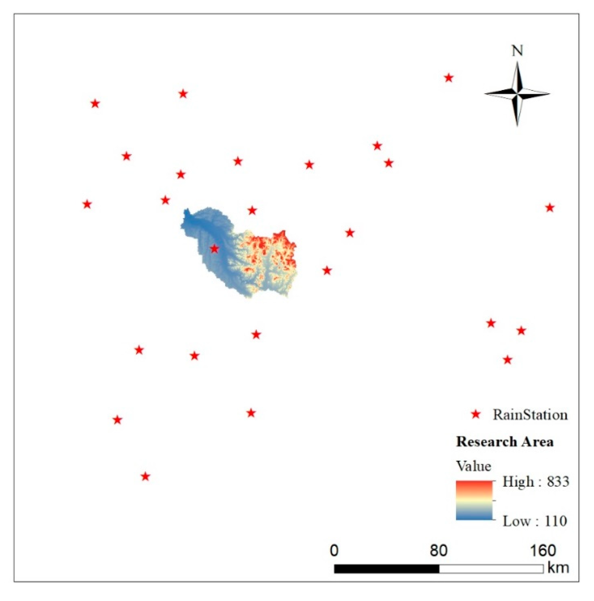
Figure 5.
Location map of meteorological stations.

Figure 6.
Flowchart of model.

Figure 7.
Comparison of runoff rate determination and validation.

Figure 8.
Comparison of total nitrogen concentration determination and validation.

Figure 9.
Comparison of total phosphorus concentration determination and validation.

Figure 10.
Land use dynamic degree.

Figure 11.
Land use change, 2000–2010. (We can compare by transfer in and transfer out, a certain kind of land transferred out will become a different land use type in the transfer in. The change in this figure is small, but the change in the later Figure 12 and Figure 13 is obvious).

Figure 12.
Land use change, 2010–2020. (Here are two different diagrams. The land use transferred from the previous image will be transferred to a different land use, which can be distinguished by color).
Figure 12.
Land use change, 2010–2020. (Here are two different diagrams. The land use transferred from the previous image will be transferred to a different land use, which can be distinguished by color).

Figure 13.
Land use change, 2000–2020. (Here are two different diagrams. The land use transferred from the previous image will be transferred to a different land use, which can be distinguished by color).
Figure 13.
Land use change, 2000–2020. (Here are two different diagrams. The land use transferred from the previous image will be transferred to a different land use, which can be distinguished by color).


Figure 14.
Annual runoff under three phases of land use.

Figure 15.
Map of monthly runoff volume changes under the three land use phases.

Figure 16.
Annual load of total nitrogen under three land use phases.

Figure 17.
Monthly loadings of total annual nitrogen under three land use phases.

Figure 18.
Average annual load per unit of total nitrogen.

Figure 19.
Annual load of total phosphorus under three land use phases.

Figure 20.
Annual total phosphorus monthly loadings under three land use phases.

Figure 21.
Average annual load of total phosphorus per unit.


Table 1.
Data sources and basic information.
| Data Name | Data Source | Data Type | Basic Information |
|---|---|---|---|
| DEM | Geospatial Data Cloud | SRTM | SRTMDEMUTM 90M |
| Land Use Map | Resource and Environmental Science and Data Center | GRID | 1 km Grid data |
| Soil type map | Resource and Environmental Science and Data Center | GRID | HWSD China Soil |
| Watershed map | Google Earth | - | - |
| Meteorology | National Weather Science Data Center | Daily Scale | 2010–2020 |
| Measured runoff data | Harbin Acheng District Hydrology Station | Monthly scale | 2015–2020 |
| Measured nitrogen and phosphorus data | Harbin City Environmental Monitoring Center | Monthly scale | 2015–2020 |
Table 2.
Soil type table.
| Number | Full Name | Soil Group |
|---|---|---|
| PHj | Stagnic Phaeozems | PHAEOZEMS |
| PHh | Haplic Phaeozems | PHAEOZEMS |
| PHg | Gleyic Phaeozems | PHAEOZEMS |
| LVh | Haplic Luvisols | LUVISOLS |
| LVg | Gleyic Luvisols | LUVISOLS |
| LVa | Albic Luvsiols | LUVISOLS |
| GLm | Mollic Gleysols | GLEYSOLS |
| ATc | Cumulic Anthrosols | ANTHROSOLS |
Table 3.
Meteorological Data.
| Number | Station Number | Longitude (°) | Latitude (°) |
|---|---|---|---|
| 1 | pcp50851 | 126.05 | 46.41 |
| 2 | pcp50853 | 126.58 | 46.37 |
| 3 | pcp50858 | 125.56 | 46.04 |
| 4 | pcp50859 | 126.17 | 46.17 |
| 5 | pcp50867 | 127.21 | 46.05 |
| 6 | pcp50877 | 129.35 | 46.18 |
| 7 | pcp50953 | 126.34 | 45.56 |
| 8 | pcp50956 | 126.46 | 46.05 |
| 9 | pcp50958 | 126.56 | 45.32 |
| 10 | pcp50960 | 127.23 | 45.44 |
| 11 | pcp50962 | 128.02 | 45.57 |
| 12 | pcp50963 | 128.44 | 45.58 |
| 13 | pcp50964 | 128.48 | 45.50 |
| 14 | pcp50965 | 128.16 | 45.26 |
| 15 | pcp50968 | 127.58 | 45.13 |
| 16 | pcp50979 | 130.14 | 45.16 |
| 17 | pcp54063 | 126.00 | 44.58 |
| 18 | pcp54065 | 125.39 | 44.32 |
| 19 | pcp54069 | 125.48 | 44.10 |
| 20 | pcp54072 | 126.31 | 44.51 |
| 21 | pcp54076 | 126.56 | 44.23 |
| 22 | pcp54080 | 127.09 | 44.54 |
| 23 | pcp54092 | 129.24 | 44.36 |
| 24 | pcp54094 | 129.40 | 44.30 |
| 25 | pcp54098 | 129.28 | 44.20 |
Table 4.
Table of evaluation coefficient effect.
| Performance Ratio | ||
|---|---|---|
| Very good | ||
| Good | ||
| Satisfactory | ||
| Unsatisfactory |
Table 5.
Meaning and value of parameters.
| Number | Parameter | Definition | Mode | Value Range | Target | Value |
|---|---|---|---|---|---|---|
| 1 | CN2 | SCS runoff curve coefficient | v | 0–200 | Runoff | 85.2109 |
| 2 | ALPHA_BF | Base-flow α coefficient | v | 0–1 | Runoff | 0.171 |
| 3 | GW_DELAY | Groundwater hysteresis factor | v | 0–500 | Runoff | 484.5 |
| 4 | GW_REVAP | Groundwater re-evaporation coefficient | v | 0–1 | Runoff | 0.1602 |
| 5 | ESCO | Soil evaporation compensation factor | v | 0–1 | Runoff | 0.201 |
| 6 | CH_N2 | Main river Manning system values | v | 0–0.31 | Runoff | 0.1595 |
| 7 | CH_K2 | Effective hydraulic conductivity of the river | v | 0.01–500 | Runoff | 91.4918 |
| 8 | ALPHA_BNK | River storage factor | v | 0–1 | Runoff | 0.543 |
| 9 | SOL_AWC | Soil water availability | v | 0–1 | Runoff | 0.665 |
| 10 | SOL_K | Saturated hydraulic conductivity | v | 0–250 | Runoff | 186 |
| 11 | SOL_BD | Wet capacity of surface soil | v | 0.5–2.5 | Runoff | 2.2424 |
| 12 | GWQMN | Shallow groundwater net flow coefficient | v | 0–5000 | Runoff | 2085 |
| 13 | SLSUBBSN | Average slope length | v | 10–100 | Runoff | 88.82 |
| 14 | OV_N | Manning factor for slope diffuse flow | v | 0–10 | Runoff | 6.0979 |
| 15 | LAT_TTIME | Soil flow measurement delay index | v | 0–100 | Runoff | 10.26 |
| 16 | NPERCO | Nitrogen permeability coefficient | v | 0–1 | Water Quality | 0.7616 |
| 17 | PPERCO | Phosphorus permeability coefficient | v | 10–17.5 | Water Quality | 12.5375 |
| 18 | PHOSKD | Soil phosphorus partition coefficient | v | 100–200 | Water Quality | 144.8333 |
| 19 | PSP | Index of phosphorus effectiveness | v | 0.01–0.7 | Water Quality | 0.5953 |
| 20 | N_UPDIS | Nitrogen absorption distribution parameters | v | 20–100 | Water Quality | 76.5 |
| 21 | P_UPDIS | Phosphorus absorption distribution parameters | v | 20–100 | Water Quality | 85.1666 |
| 22 | FIXCO | Nitrogen fixation factor | v | 0–1 | Water Quality | 0.9516 |
| 23 | SHALLST_N | Nitrate concentration in groundwater runoff | v | 0–1000 | Water Quality | 715 |
| 24 | GWSOLP | Groundwater soluble phosphorus concentration | v | 0–1000 | Water Quality | 951.6666 |
| 25 | HLIFE_NGW | Half-life of nitrogen | v | 0–200 | Water Quality | 114.3333 |
| 26 | LAT_ORGN | Baseflow organic nitrogen content | v | 0–200 | Water Quality | 1.6666 |
| 27 | LAT_ORGP | Basestream organophosphorus content | v | 0–200 | Water Quality | 3.6666 |
| 28 | BIOMIX | Biomixing efficiency | v | 0–1 | Water Quality | 0.9016 |
| 29 | CH_ONCO | Concentration of organic nitrogen in the river | v | 0–100 | Water Quality | 43.5 |
| 30 | CH_OPCO | Concentration of organic phosphorus in the river | v | 0–100 | Water Quality | 23.1666 |
| 31 | ERORGP | Organic phosphorus enrichment rate | v | 0–5 | Water Quality | 0.2583 |
| 32 | POT_NO3L | Nitrate decay rate in potholes | v | 0–1 | Water Quality | 0.425 |
| 33 | ORGN_CON | Organic nitrogen concentration in runoff | v | 0–100 | Water Quality | 9.5 |
| 34 | ORGP_CON | Organic phosphorus concentration in runoff | v | 0–50 | Water Quality | 14.5833 |
| 35 | ERORGN | Enrichment rate of organic nitrogen | v | 0–5 | Water Quality | 2.255 |
Table 6.
Land use change area statistics of Ashe River Basin from 2000 to 2020 (km2).
| Land Type | 2000 | 2010 | 2020 | 2000~2010 | 2010~2020 | 2000~2020 | |||
|---|---|---|---|---|---|---|---|---|---|
| Area | Area | Area | Variation | K | Variation | K | Variation | K | |
| Cropland | 1668.11 | 1640.77 | 1567.82 | −27.34 | −0.16% | −72.95 | −0.44% | −100.29 | −0.30% |
| Forest | 1567.72 | 1585.61 | 1547.16 | 17.89 | 0.11% | −38.45 | −0.24% | −20.56 | −0.07% |
| Grassland | 46.03 | 41.72 | 29.01 | −4.31 | −0.94% | −12.71 | −3.05% | −17.02 | −1.85% |
| Water | 31.36 | 30.33 | 32.7 | −1.03 | −0.33% | 2.37 | 0.78% | 1.34 | 0.21% |
| Urban | 177.8 | 192.61 | 269.87 | 14.81 | 0.83% | 77.26 | 4.01% | 92.07 | 2.59% |
| Unused Land | 9.94 | 9.94 | 54.44 | 0 | 0.00% | 44.5 | 44.77% | 44.5 | 22.38% |
| Total area | 3501 | ||||||||
Table 7.
Land Use Transfer Matrix 2000~2010 (km2).
| 2000 Transfer out | ||||||||
|---|---|---|---|---|---|---|---|---|
| Cropland | Forest | Grassland | Water | Urban | Unused Land | 2010 Total | ||
| 2010 Transfer to | Cropland | 1638.69 | 1.04 | 1.04 | 0 | 0 | 0 | 1640.77 |
| Forest | 10.91 | 1564.60 | 10.10 | 0 | 0 | 0 | 1585.61 | |
| Grassland | 5.78 | 1.04 | 34.89 | 0 | 0 | 0 | 41.72 | |
| Water | 0 | 0 | 0 | 30.32 | 0 | 0 | 30.33 | |
| Urban | 12.73 | 1.04 | 0 | 1.04 | 177.80 | 0 | 192.61 | |
| Unused Land | 0 | 0 | 0 | 0 | 0 | 9.94 | 9.94 | |
| 2000 Total | 1668.11 | 1567.72 | 46.03 | 31.36 | 177.80 | 9.94 | 3501 | |
Table 8.
Land Use Transfer Matrix 2010~2020 (km2).
| 2010 Transfer out | ||||||||
|---|---|---|---|---|---|---|---|---|
| Cropland | Forest | Grassland | Water | Urban | Unused Land | 2020 Total | ||
| 2020 Transfer to | Cropland | 1236.47 | 221.86 | 12.60 | 1.93 | 94.57 | 0.37 | 1567.82 |
| Forest | 188.19 | 1316.23 | 23.93 | 6.32 | 10.93 | 1.86 | 1547.16 | |
| Grassland | 12.63 | 10.24 | 2.73 | 0 | 3.40 | 0 | 29.01 | |
| Water | 12.42 | 3.58 | 0 | 11.59 | 0.09 | 5.02 | 32.70 | |
| Urban | 161.90 | 20.57 | 1.51 | 5.39 | 80.50 | 0.01 | 269.87 | |
| Unused Land | 28.48 | 14.94 | 0.86 | 5.03 | 2.74 | 2.69 | 54.44 | |
| 2010 Total | 1640.77 | 1585.61 | 41.71 | 30.33 | 192.61 | 9.94 | 3501 | |
Table 9.
Land Use Transfer Matrix 2000~2020 (km2).
| 2000 Transfer out | ||||||||
|---|---|---|---|---|---|---|---|---|
| Cropland | Forest | Grassland | Water | Urban | Unused Land | 2000 Total | ||
| 2020 Transfer to | Cropland | 1247.24 | 217.01 | 10.29 | 1.93 | 90.97 | 0.37 | 1567.82 |
| Forest | 191.07 | 1305.03 | 33.29 | 6.32 | 9.88 | 1.86 | 1547.16 | |
| Grassland | 15.36 | 10.24 | 0.01 | 0 | 3.40 | 0 | 29.01 | |
| Water | 13.30 | 2.70 | 0 | 11.59 | 0.09 | 5.02 | 32.7 | |
| Urban | 171.82 | 19.77 | 1.51 | 6.27 | 70.50 | 0.01 | 269.87 | |
| Unused Land | 28.65 | 14.77 | 0.88 | 5.19 | 2.58 | 2.69 | 54.44 | |
| 2020 Total | 1668.11 | 1567.72 | 46.03 | 31.36 | 177.80 | 9.94 | 3501 | |
Publisher’s Note: MDPI stays neutral with regard to jurisdictional claims in published maps and institutional affiliations. |
© 2022 by the authors. Licensee MDPI, Basel, Switzerland. This article is an open access article distributed under the terms and conditions of the Creative Commons Attribution (CC BY) license (https://creativecommons.org/licenses/by/4.0/).
Share and Cite
MDPI and ACS Style
Chen, J.; Du, C.; Nie, T.; Han, X.; Tang, S. Study of Non-Point Pollution in the Ashe River Basin Based on SWAT Model with Different Land Use. Water 2022, 14, 2177. https://doi.org/10.3390/w14142177
AMA Style
Chen J, Du C, Nie T, Han X, Tang S. Study of Non-Point Pollution in the Ashe River Basin Based on SWAT Model with Different Land Use. Water. 2022; 14(14):2177. https://doi.org/10.3390/w14142177
Chicago/Turabian StyleChen, Jiashuo, Chong Du, Tangzhe Nie, Xu Han, and Siyu Tang. 2022. "Study of Non-Point Pollution in the Ashe River Basin Based on SWAT Model with Different Land Use" Water 14, no. 14: 2177. https://doi.org/10.3390/w14142177
Note that from the first issue of 2016, this journal uses article numbers instead of page numbers. See further details here.