Climate Change Impacts on Stream Water Temperatures in a Snowy Cold Region According to Geological Conditions

Abstract

This study clarifies how climate change affects stream temperatures in snowy cold regions, where groundwater impacts vary with geological conditions. We developed a physics-based water circulation model that incorporates an atmospheric and land surface process model considering snow processes, a runoff model, and a water temperature estimation model. Small watersheds in the mountainous area of Hokkaido formed the study area, and the runoff model was assigned different parameters depending on the geological characteristics. Using these parameters, changes in water temperature were calculated with respect to changes in the meteorological data in historical and future simulations. Current water temperatures were effectively reproduced by the model, and following the IPCC RCP 8.5 scenario, future water temperatures in the distribution area for new pyroclastic flows were predicted to remain lower in summer than in the distribution area of older formations. The findings of this study will be useful in informing conservation measures for river ecosystems, including the prioritization of streams where cold-water fish need to be conserved.

1. Introduction

In recent decades, increases in stream water temperature have been observed in regions worldwide [1,2,3,4,5]. These are expected to continue increasing in the future with climate change [6,7,8,9,10]. Changes in the timing and amount of snowmelt contribute to changes in water temperature in streams in snowy cold regions [10,11]. Many researchers are concerned that rising water temperatures associated with climate change will have a range of impacts [6] including water quality degradation [12] and changes to cooling water for power generation [13]. In snowy cold regions, the impact of rising water temperatures on stream ecosystems has become a major problem, and suitable habitats for cold-water fish species, such as salmonids, are likely to shrink in size [7,10]. Attention has been focused on adaptation measures for conservation, such as identifying favorable areas for the survival of cold-water fish where summer water temperatures will remain cooler under climate change [14,15]. For detailed adaptation considerations, it is important to predict detailed responses of stream water temperature to climate change.

Stream water temperatures depend on a range of factors related to atmospheric conditions, topography, discharge and the streambed, with groundwater input being a key factor [16]. Previous studies using weekly and monthly data have indicated that in groundwater-dominant streams, the change in water temperature in response to changes in the air temperature is smaller than in non-groundwater-dominant streams [16]. The contribution of groundwater to a stream can be highly dependent on geologic conditions of the watershed [17]. Therefore, differences in the geologic conditions can be an important factor controlling the water temperature in a watershed [18].

Ishiyama et al. [19] demonstrated via a statistical analysis of historical data that watershed geology with a high groundwater contribution creates refugia for cold-water species under current and warming climate conditions. However, the effects of future climate change cannot always be fully predicted by statistical analysis. In snowy cold regions, future snowpack loss will increase the temperature of the cold water in streams [9,10]. Studies based on the statistical analysis of historical data do not always adequately account for this effect [20]. To improve the rigorous discussion of future projections, physics-based models that take physical processes into account will likely be introduced [19,20]. Although several studies [7,8,10,20] have used physics-based models to predict future water temperatures in snowy cold regions, none of them have examined specific water temperature increases under different geological conditions.

The purpose of this study is to clarify how stream water temperatures change with climate change among streams in snowy cold regions, where the influence of groundwater varies with geological conditions. Model predictions based on physics-based models were made for small watersheds with contrasting geological conditions, applying different parameters for each geological property to show the differences in the discharge and water temperatures between watersheds.

2. Study Area and Methods

2.1. Study Area

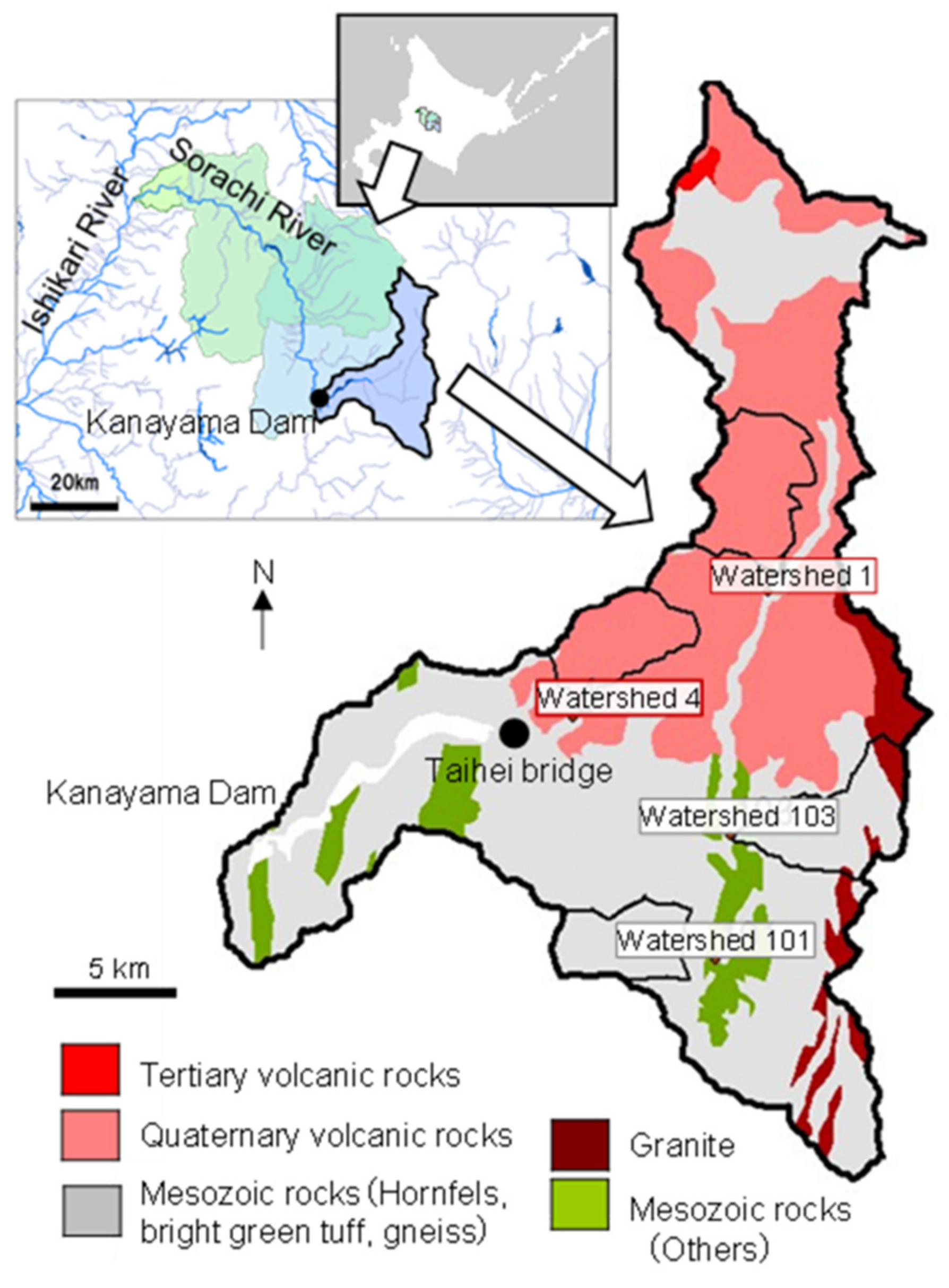
The study area is the Kanayama Dam watershed (watershed area: 470 km²) located in the uppermost reaches of the Sorachi River in the Ishikari River system in Hokkaido (main channel length: 194.5 km, watershed area: 2618 km²) [21]. The Sorachi River originates on the southern slope of Mt. Kamihorokametok and flows into the Kanayama Dam Reservoir (Lake Kanayama) via the Taihei bridge (watershed area: 381 km²). Four subwatersheds of the Sorachi River tributaries that are mainly forested (hereafter referred to as watershed 1, 4, 101, and 103), the Kanayama dam, and the Taihei bridge approximately 12 km upstream of the Kanayama Dam were selected as sites for calculating the stream discharge and the water temperature. The outline and geological composition of the study area are shown in Figure 1 and Table 1. Watersheds 1 and 4 are mainly covered by Tokachi pyroclastic flow deposits from the Quaternary [22] (hereafter referred to as “Quaternary pyroclastic flow”), while watersheds 101 and 103 have predominantly Mesozoic formations (Hidaka group or Hidaka metamorphic or plutonic rocks [22], hereafter referred to as “Mesozoic rocks”). Near the Kanayama Dam, Sakhalin taimen (Hucho perryi) and Cherry salmon (Oncorhynchus masou), cold water salmonids listed as endangered species in Japan, have been confirmed to be present.

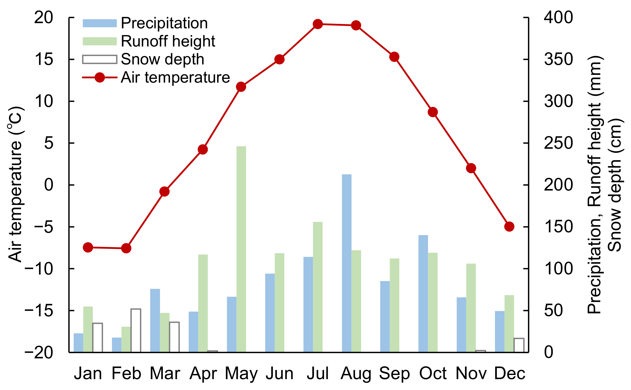
Monthly trends in average air temperature, precipitation, average snow depth, and runoff height in the study area are shown in Figure 2. In Hokkaido, the southeast monsoon brings warm air from the North Pacific in summer, while the prevailing northwest wind provides cold air from Siberia in winter, resulting in large annual temperature differences [23]. Since the study area is located inland, low temperatures are prominent in winter, with average monthly temperatures below −5 °C from December to February. Monthly precipitation is relatively high from summer to autumn, when the area is susceptible to fronts and typhoons. Winter precipitation is mainly observed as snow, with the average snow depth in February reaching approximately 50 cm, and the snow cover period ranging from November to April. Due to the melting and runoff of snow accumulated during winter, the monthly average runoff height is highest during spring in May.

Figure 1. Location and geological composition of the study area. For the geological classification, we used the method by Usutani et al. [24] based on the classification of Mushiake et al. [25].

Figure 1. Location and geological composition of the study area. For the geological classification, we used the method by Usutani et al. [24] based on the classification of Mushiake et al. [25].

2.2. Observation Data

Hourly water level and temperature data (13 March 2018–30 September 2019) were observed in the four subwatersheds using a data logger (CO-U20L-04, Onset Computer Corporation, Bourne, MA, USA) and used to verify the reproducibility of the stream discharge and temperatures in the watersheds (Table 1). Water levels in watershed 101 from 13 March to 30 June 2018 were excluded because the specific discharge calculated was underestimated compared with the other watersheds.

The hourly water level was converted into hourly stream discharge based on Manning’s average flow velocity and on field observations made at the water level observation points in each subwatershed on 23 September 2020 and were arranged as daily values. Manning’s average flow velocity is given by Equation (1):

$$\mathrm{v}=\frac{1}{\mathrm{n}}{\mathrm{R}}^{2/3}{\mathrm{i}}^{1/2}$$

(1)

where v is the cross-sectional mean velocity (m/s), n is Manning’s roughness coefficient (${\mathrm{m}}^{-1/3}\mathrm{s}$), R is the radial depth (m), and i is the energy gradient. The energy gradient is assumed to be equal to the bed gradient.

The cross-sectional profile of the channel, channel gradient i, R, stream cross-sectional area A, and stream discharge Q were investigated at watersheds 1, 4, 101, and 103 on 23 September 2020. Parameter i was calculated for each stream channel based on a 30–40 m longitudinal survey, and Q was calculated based on velocity observations using an electromagnetic current meter (AEM1-DA, JFE Advantech Corporation, Nishinomiya, Japan) and a cross-sectional survey. Parameter n was calculated by substituting i, R, and v (= Q/A) from field observations into Equation (1). The parameters i and n calculated for each stream are shown in Table 2. A and R corresponding to the observed water levels and cross-sections of the stream were calculated hourly for each day. Both this R and i and n obtained above were substituted into Equation (1) and multiplied by A to calculate the hourly stream discharge Q.

Table 1. Watersheds for stream discharge and water temperature observations.

Watershed (Location)	Major Constituent Geology	Watershed Area (km2)	Observation Data of Discharge and Water Temperature	Calculation Method or Source
Watershed 1	Quaternary pyroclastic flow deposits (Tokachi pyroclastic flow deposits)	21.9	From 13 March 2018 to 30 September 2019	Stream discharge: After measuring the water level with a data logger, convert it to discharge using Manning’s formula. Water temperature: measured with a data logger
Watershed 4	Quaternary pyroclastic flow deposits (Tokachi pyroclastic flow deposits)	16.4	From 13 March 2018 to 30 September 2019	Stream discharge: After measuring the water level with a data logger, convert it to discharge using Manning’s formula. Water temperature: measured with a data logger
Watershed 101	Mesozoic rocks (Hornfels, bright green tuff, gneiss)	17.1	From 13 March 2018 to 30 September 2019 Treat as missing data from 13 March 2018 to 30 June 2018	Stream discharge: After measuring the water level with a data logger, convert it to discharge using Manning’s formula. Water temperature: measured with a data logger
Watershed 103	Mesozoic rocks (Hornfels, bright green tuff, gneiss)	20.4	From 13 March 2018 to 30 September 2019	Stream discharge: After measuring the water level with a data logger, convert it to discharge using Manning’s formula. Water temperature: measured with a data logger
Kanayama Dam	Quaternary pyroclastic flow deposits and Mesozoic rocks	470	From 13 March 2018 to 30 September 2019 (Stream discharge only)	Published by the Ministry of Land, Infrastructure, Transport, and Tourism [26]
Taihei bridge	Quaternary pyroclastic flow deposits and Mesozoic rocks	381	13 measurement data (Water temperature only)	Published by the Ministry of Land, Infrastructure, Transport, and Tourism [26]

Table 1. Watersheds for stream discharge and water temperature observations.

Watershed (Location)	Major Constituent Geology	Watershed Area (km2)	Observation Data of Discharge and Water Temperature	Calculation Method or Source
Watershed 1	Quaternary pyroclastic flow deposits (Tokachi pyroclastic flow deposits)	21.9	From 13 March 2018 to 30 September 2019	Stream discharge: After measuring the water level with a data logger, convert it to discharge using Manning’s formula. Water temperature: measured with a data logger
Watershed 4	Quaternary pyroclastic flow deposits (Tokachi pyroclastic flow deposits)	16.4	From 13 March 2018 to 30 September 2019	Stream discharge: After measuring the water level with a data logger, convert it to discharge using Manning’s formula. Water temperature: measured with a data logger
Watershed 101	Mesozoic rocks (Hornfels, bright green tuff, gneiss)	17.1	From 13 March 2018 to 30 September 2019 Treat as missing data from 13 March 2018 to 30 June 2018	Stream discharge: After measuring the water level with a data logger, convert it to discharge using Manning’s formula. Water temperature: measured with a data logger
Watershed 103	Mesozoic rocks (Hornfels, bright green tuff, gneiss)	20.4	From 13 March 2018 to 30 September 2019	Stream discharge: After measuring the water level with a data logger, convert it to discharge using Manning’s formula. Water temperature: measured with a data logger
Kanayama Dam	Quaternary pyroclastic flow deposits and Mesozoic rocks	470	From 13 March 2018 to 30 September 2019 (Stream discharge only)	Published by the Ministry of Land, Infrastructure, Transport, and Tourism [26]
Taihei bridge	Quaternary pyroclastic flow deposits and Mesozoic rocks	381	13 measurement data (Water temperature only)	Published by the Ministry of Land, Infrastructure, Transport, and Tourism [26]

Figure 2. Monthly average air temperature, precipitation, runoff height, and snow depth in the study area. Air temperature, precipitation, and snow depth correspond to the 2018–2020 average at the JMA Ikutora observatory (AMeDAS) [27]; runoff height is the 2018–2020 average for the Sorachi River at the Taihei bridge [26].

Figure 2. Monthly average air temperature, precipitation, runoff height, and snow depth in the study area. Air temperature, precipitation, and snow depth correspond to the 2018–2020 average at the JMA Ikutora observatory (AMeDAS) [27]; runoff height is the 2018–2020 average for the Sorachi River at the Taihei bridge [26].

Table 2. Streambed gradient i and Manning roughness coefficient n for each subwatershed obtained by field observations.

Watershed	i	n
Watershed 1	0.0170	0.166
Watershed 4	0.0108	0.128
Watershed 101	0.0246	0.070
Watershed 103	0.0179	0.083

Table 2. Streambed gradient i and Manning roughness coefficient n for each subwatershed obtained by field observations.

Watershed	i	n
Watershed 1	0.0170	0.166
Watershed 4	0.0108	0.128
Watershed 101	0.0246	0.070
Watershed 103	0.0179	0.083

The daily inflow at the Kanayama Dam and 13 water temperature measurements at the Taihei bridge, published by The Ministry of Land, Infrastructure, Transport and Tourism [26], were used to verify the reproducibility of the discharge and water temperature calculated by the model. The observed water temperature at the Taihei bridge deviates from the daily average water temperature because it is observed at specific times during the day. In FY2021, the water temperature at the Taihei bridge was continuously measured with a water temperature sensor, and the difference between the average water temperature at each time of the day and the daily average water temperature was calculated for each month. Assuming that this difference was also present on the day of observation, the water temperature at the time of observation was converted to the daily average water temperature.

2.3. Meteorological Data and Climate Scenario

Meteorological data including precipitation and air temperature for each approximately 1 km square mesh were used as input data for the model calculations. The sources of the data and other details are shown in Table 3 for the reproduction of current conditions and in Table 4 for historical and future climate simulations.

Table 3. The meteorological data for current situation reproduction (March 2018–September 2019).

Meteorological Factors	Units	Data Used, Spatial and Temporal Resolution
Precipitation	mm	Radar rain gauge analyzed precipitation by Japan Meteorological Agency (JMA) 1 km, hourly
Air temperature	K	Local forecast model (LFM) data by JMA, 5 km, hourly
Wind speed	m/s	Local forecast model (LFM) data by JMA, 5 km, hourly
Relative humidity	%	Local forecast model (LFM) data by JMA, 5 km, hourly
Amount of snowfall	mm	The model value by the Japan Weather Association SYNFOS-3D, 5 km, every 3 h
Total cloud cover	%	The model value by JMA SYNFOS-3D, corrected by the relational expression between the model value and the observed value at the Asahikawa Local Meteorological Observatory, 5 km, every 3 h
Lower cloud cover	%	The model value by JMA SYNFOS-3D, corrected by the same relational expression as the correction of the total cloud cover, 5 km, every 3 h

Table 3. The meteorological data for current situation reproduction (March 2018–September 2019).

Meteorological Factors	Units	Data Used, Spatial and Temporal Resolution
Precipitation	mm	Radar rain gauge analyzed precipitation by Japan Meteorological Agency (JMA) 1 km, hourly
Air temperature	K	Local forecast model (LFM) data by JMA, 5 km, hourly
Wind speed	m/s	Local forecast model (LFM) data by JMA, 5 km, hourly
Relative humidity	%	Local forecast model (LFM) data by JMA, 5 km, hourly
Amount of snowfall	mm	The model value by the Japan Weather Association SYNFOS-3D, 5 km, every 3 h
Total cloud cover	%	The model value by JMA SYNFOS-3D, corrected by the relational expression between the model value and the observed value at the Asahikawa Local Meteorological Observatory, 5 km, every 3 h
Lower cloud cover	%	The model value by JMA SYNFOS-3D, corrected by the same relational expression as the correction of the total cloud cover, 5 km, every 3 h

Table 4. Specifications of the 1 km downscaled data used to estimate climate change (1984–2004 and 2080–2100). DSJRA-55 was used as the bias correction reference data for each meteorological element except for air temperature, and 30-year average mesh climate data were used as bias correction reference data for the air temperature.

Elements	Units	Original Source of Data
Precipitation	mm	1 km mesh daily data from Ueda [28] Spatially detailed climate change projection data based on MRI-NHRCM20 (JMA) [29], after RCP 8.5 (IPCC) emission scenarios Bias correction based on DSJRA-55 and mesh climate data of 30-year average by JMA
Air temperature	K
Wind speed	m/s
Relative humidity	%
Amount of snowfall	mm
Total cloud cover	%
Lower cloud cover	%

Table 4. Specifications of the 1 km downscaled data used to estimate climate change (1984–2004 and 2080–2100). DSJRA-55 was used as the bias correction reference data for each meteorological element except for air temperature, and 30-year average mesh climate data were used as bias correction reference data for the air temperature.

Elements	Units	Original Source of Data
Precipitation	mm	1 km mesh daily data from Ueda [28] Spatially detailed climate change projection data based on MRI-NHRCM20 (JMA) [29], after RCP 8.5 (IPCC) emission scenarios Bias correction based on DSJRA-55 and mesh climate data of 30-year average by JMA
Air temperature	K
Wind speed	m/s
Relative humidity	%
Amount of snowfall	mm
Total cloud cover	%
Lower cloud cover	%

For the reproduction of the current conditions, we used data produced by the Hokkaido Branch of the Japan Weather Association that was spatially intercalated using a distance-weighted method and downscaled from a spatial resolution of 5 km to 1 km.

For past and future simulations, 1 km downscaled data by Ueda et al. [25] from 1 September 1984 to 31 August 2004 (“historical climate”) and from 1 September 2080 to 31 August 2100 (“future climate”) were used. For the future climate, we followed the representative concentration pathway (RCP) 8.5 emission scenario by the IPCC [30] and used the averages of the three patterns of sea surface temperature presented by Mizuta et al. [31]. For the historical and future climates, the first year of the 20-year analysis period was set as the run-up period and was excluded from the study. Details of the downscaling of the data set, elevation correction, and bias correction are described in Ueda et al. [32].

2.4. Atmospheric and Land Surface Process Model Considering Snow Cover Change

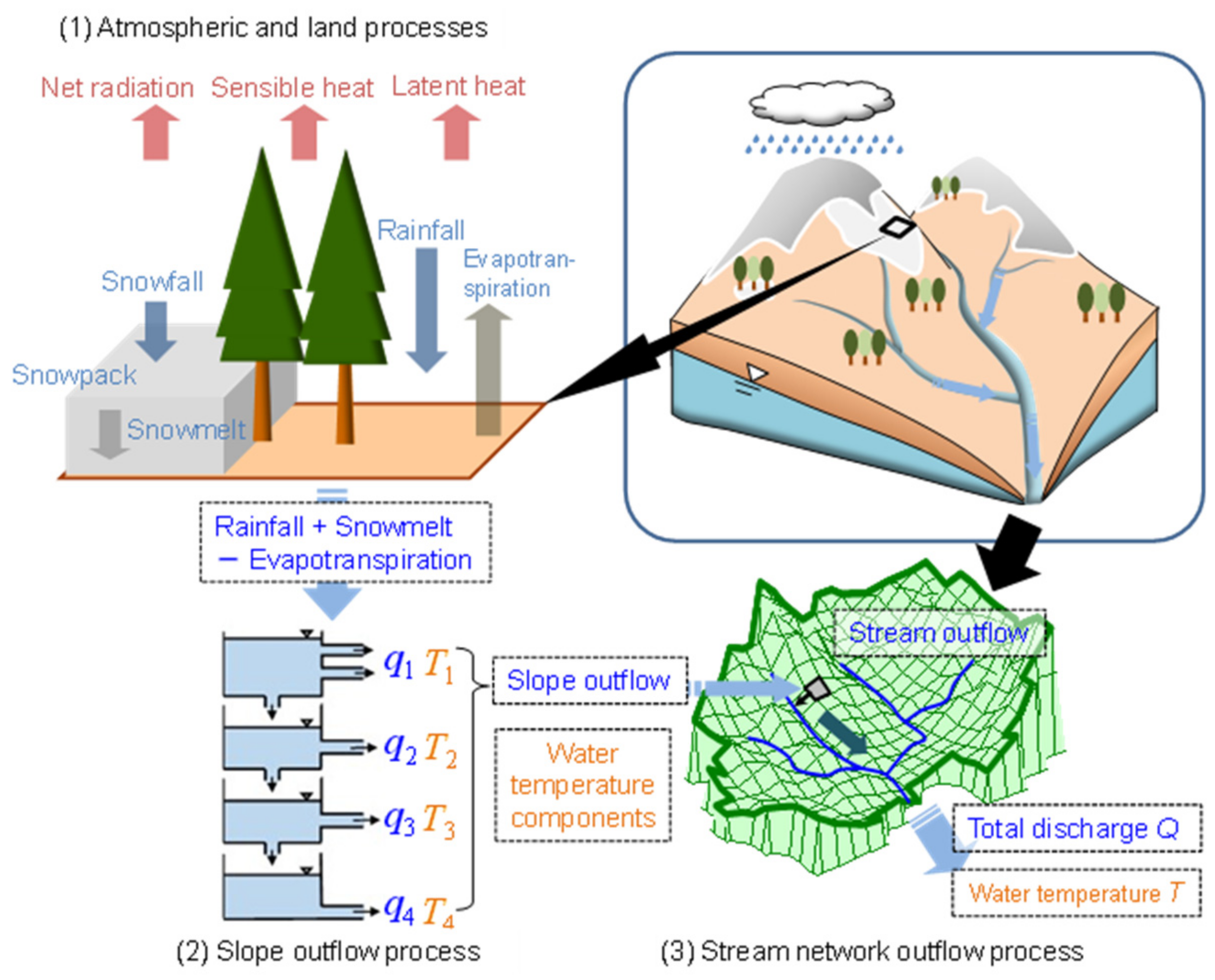
Using the 1 km downscaling data as input values, daily evapotranspiration and snowmelt were calculated using an atmospheric and land surface process model by Usutani et al. [33] incorporating snow accumulation and snowmelt (Figure 3). Equations (2) and (3), which were based on the two-layer model by Kondo [34], were used to calculate the heat flux [35,36]:

$${\mathrm{f}}_{\mathrm{v}}\mathrm{R}\downarrow +\left(1-{\mathrm{f}}_{\mathrm{v}}\right){\mathsf{\sigma }\mathrm{T}}_{\mathrm{v}}^4-{\mathrm{Q}}_{\mathrm{G}}+{\mathrm{Q}}_{\mathrm{R}}=\mathsf{\epsilon }{\mathsf{\sigma }\mathrm{T}}_{\mathrm{g}}^4+{\mathrm{H}}_{\mathrm{g}}+{\mathrm{lE}}_{\mathrm{g}}$$

(2)

$$\left(1-{\mathrm{f}}_{\mathrm{v}}\right)(\mathrm{R}\downarrow +\mathsf{\epsilon }{\mathsf{\sigma }\mathrm{T}}_{\mathrm{g}}^4)=2\left(1-{\mathrm{f}}_{\mathrm{v}}\right){\mathsf{\sigma }\mathrm{T}}_{\mathrm{v}}^4+{\mathrm{H}}_{\mathrm{v}}+\mathrm{l}\begin{array}{c}\left({\mathrm{E}}_{\mathrm{v}}+\mathrm{I}\right)\end{array}$$

(3)

where ${\mathrm{f}}_{\mathrm{v}}$ is the transmissivity of the vegetation estimated for each month, $\mathrm{R}\downarrow$ is the downward net radiation (W/m²), Q_G is the heat flux provided to the ground surface (W/m²), Q_R is the heat flux provided by rainfall (W/m²), H_g is the sensible heat flux from the ground surface including the snow surface (W/m²), H_v is the sensible heat flux from the vegetation layer (W/m²), ${\mathrm{lE}}_{\mathrm{g}}$ is the latent heat flux from the ground surface including the snow surface (W/m²), ${\mathrm{lE}}_{\mathrm{v}}$ is the latent heat flux from the vegetation layer (W/m²), $\mathrm{lI}$ is the evaporation due to interception (W/m²), ${\mathrm{T}}_{\mathrm{g}}$ is the mean temperature of the ground surface including the snow surface (K), ${\mathrm{T}}_{\mathrm{v}}$ is the mean temperature of the vegetation layer (K), $\mathsf{\epsilon }$ is the emissivity (1.00 on the ground and 0.97 on the snow cover surface), and $\mathsf{\sigma }$ is the Stefan–Boltzmann coefficient ($5.67\times {10}^{-8}$ W/m²/K⁴). Specific calculations for Equations (2) and (3) were performed according to Kuchizawa and Nakatsugawa [35] and Nakatsugawa and Hoshi [36].

2.5. Runoff Model

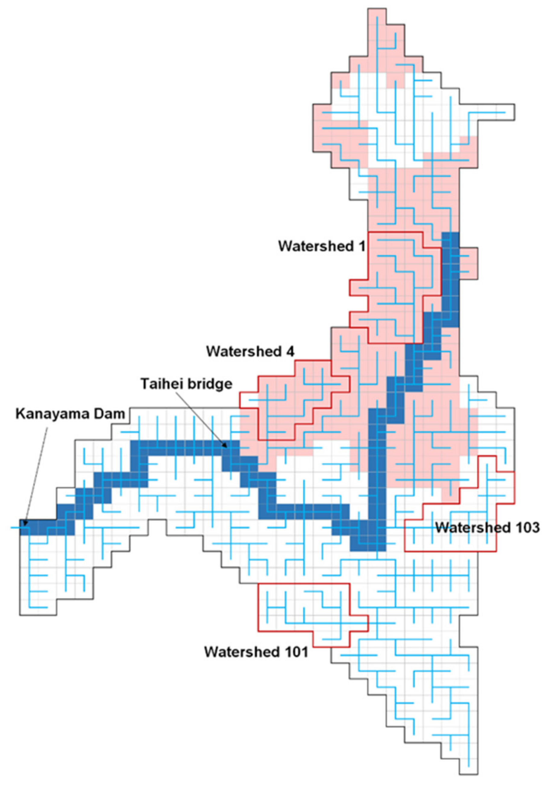
A distributed runoff model that combines slope runoff and stream channel routing by Usutani et al. [33] was applied to estimate the stream discharge. Information from the Foundation of Hokkaido River Disaster Prevention Research Center [37] was used as the distribution of the stream channel network (Figure 4). The daily slope runoff was calculated using the four-stage tank model, which is a conceptual rainfall runoff model by Sugawara [38]. For each mesh downstream of the uppermost reaches of the watershed, the inflow from upstream was added to the slope runoff, and the stream discharge was calculated through channel tracking.

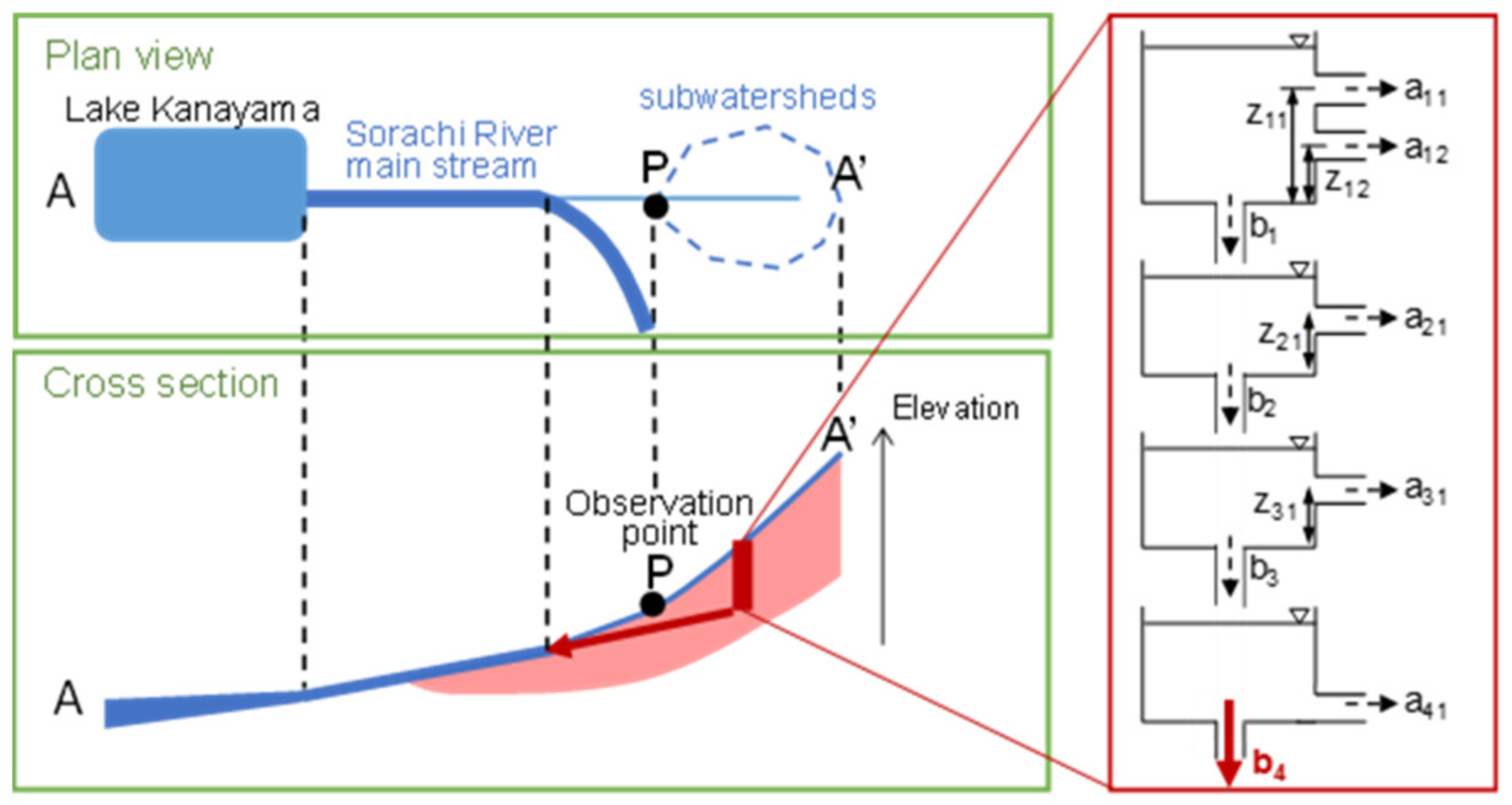
The effective precipitation amount obtained by subtracting the evapotranspiration amount from the rainfall amount and the snowmelt amount for each mesh was input to the four-stage tank model, and the runoff amount for each tank was totaled to calculate the amount of slope runoff. However, in watersheds 1 and 4 of the pyroclastic flow deposits, the stream discharge was much smaller than the effective precipitation, and the stream discharge could not be reproduced by the calculation using the general four-stage tank model. This was interpreted as groundwater becoming subterranean and flowing further downstream in areas where pyroclastic flow deposits are distributed. To account for this effect, a bottom outlet was added to the fourth tank of the tank model in watersheds 1 and 4, and it was assumed that the volume of water infiltrating through the bottom outlet would flow out at the uppermost mesh corresponding to the main channel of the Sorachi River (the area colored blue in Figure 4) downstream of the watershed (Figure 5).

The tank model parameters were searched for each subwatershed using the SCE-UA method by Duan et al. [39], a proven optimization method used for tank model parameter estimation [40], and then adjusted by trial and error to obtain the optimal values, so that the water balance of the watershed could also be consistently explained. Outside the watersheds where observations were made, the mean values for watersheds 1 and 4 were applied for watersheds with pyroclastic flow deposits, and the values for watershed 103 for watersheds with Mesozoic rocks were applied as the tank model parameters.

Figure 4. The stream channel network used for the distributed runoff model (after [37]). The blue area comprises the main channel of the Sorachi River.

Figure 4. The stream channel network used for the distributed runoff model (after [37]). The blue area comprises the main channel of the Sorachi River.

Figure 5. Assumption of the recharged water movements for watersheds with pyroclastic flow deposits (watersheds 1 and 4). The volume of water infiltrating through the bottom outlet (penetration coefficient: b₄) added to the fourth tank of the tank model would flow out at the mesh corresponding to the main channel of the Sorachi River (Figure 4).

Figure 5. Assumption of the recharged water movements for watersheds with pyroclastic flow deposits (watersheds 1 and 4). The volume of water infiltrating through the bottom outlet (penetration coefficient: b₄) added to the fourth tank of the tank model would flow out at the mesh corresponding to the main channel of the Sorachi River (Figure 4).

For stream channel routing, the cross-section profile of the stream channel is regarded as a wide rectangle, with the stream channel flow being regarded as a one-dimensional unsteady gradual change flow of the open channel. Kinematic approximation is applied considering the stream gradient in the main watershed as a steep gradient exceeding 1/1000, and Equation (4) was calculated by the finite difference method using the forward difference as the time-derivative term and the backward difference as the spatial-derivative term:

$$\frac{\partial \mathrm{A}}{\partial \mathrm{t}}+\frac{\partial \mathrm{Q}}{\partial \mathrm{x}}={\mathrm{q}}_{\mathrm{L}}$$

(4)

Q and A are the stream discharge (m³/s) and the cross-sectional area of the stream channel (m²), and ${\mathrm{q}}_{\mathrm{L}}$ is the inflow from the slope per unit time and unit length of the stream channel (m²/s).

Q was calculated by multiplying the cross-sectional average flow velocity v obtained by Equation (4) by A. Of the parameters required in Equation (4), the streambed gradient i was calculated from the elevation difference between the target mesh and the lowest elevation of its downstream mesh. The elevation data were sourced from the Foundation of Hokkaido River Disaster Prevention Research Center [37]. Manning’s roughness coefficient n was set to the values in Table 2 in the watersheds where field observations were made, while it was set to 0.147 (average of watersheds 1 and 4) for pyroclastic flow deposits and 0.083 (watershed 103) for Mesozoic rocks in the other subwatersheds. In the main channel of the Sorachi River (the section of the mesh colored in blue in Figure 4), n was uniformly set to 0.05. The diameter depth R of the stream was approximated by considering it to be equal to stream width B. B was derived using Equations (5) and (6) on a daily basis, assuming that it can be expressed as a function of ${\mathrm{Q}}_{\mathrm{in}}$, the stream discharge flowing into the mesh from upstream on a daily basis, referring to the empirical findings in Leopold and Maddock [41] and Arai and Nishizawa [42]:

$$\mathrm{B}=5.5{\mathrm{Q}}_{\mathrm{in}}{}^{0.18} (\mathrm{u}\le 4)$$

(5)

$$\mathrm{B}=10.7{\mathrm{Q}}_{\mathrm{in}}{}^{0.42} \left(\mathrm{u}\ge 5\right)$$

(6)

Here, u is the water flow order of Strahler [43] based on the interpretation of the 1/25,000 topographic map by the Geospatial Information Authority of Japan. The section of u ≥ 5 corresponds with the main channel of the Sorachi River (the section of the blue grid section in Figure 4). Coefficient ${\mathrm{Q}}_{\mathrm{in}}$ was set based on the relationship between the stream width and the stream discharge in the field observations from the four subwatersheds when u ≤ 4 and on the relationship between the stream width and the stream discharge calculated (median during the target period) for each mesh in the main channel of the Sorachi River measured from aerial photographs on Google Earth [44] when u ≥ 5.

To evaluate the reproducibility of the stream discharge, Nash–Sutcliffe coefficients (NSEs) [45] were calculated for the study period, excluding missing days, and referred to as quantitative indicators.

2.6. Water Temperature Estimation Model

Regarding the stream water temperature, the product of the stream discharge and the water temperature is defined as the water temperature flux (m³/s·K), referring to Kudo et al. [7]. The water temperature fluxes were added sequentially with channel routing, and the water temperature flux was divided by the stream discharge to calculate the water temperature for each day and each mesh. A conceptual diagram of the stream water temperature estimation is shown in Figure 6.

The water temperature flux estimation formulas for each outflow component from the slope are shown in Equations (7)–(11). ${\mathsf{\phi }}_{4\mathrm{i}}$ for the future climate is calculated separately in two patterns:

$${\mathsf{\phi }}_{1\mathrm{i}}={\mathrm{q}}_{1\mathrm{i}}({\mathrm{T}}_{\mathrm{d}}+273.15)$$

(7)

$${\mathsf{\phi }}_{2\mathrm{i}}={\mathrm{q}}_{2\mathrm{i}}\left\{{\mathrm{p}}_2\frac{{\mathsf{\phi }}_{1\mathrm{i}}}{{\mathrm{q}}_{1\mathrm{i}}}+\left(1-{\mathrm{p}}_2\right)\frac{{\mathsf{\phi }}_{4\mathrm{i}}}{{\mathrm{q}}_{4\mathrm{i}}}\right\}$$

(8)

$${\mathsf{\phi }}_{3\mathrm{i}}={\mathrm{q}}_{3\mathrm{i}}\left\{{\mathrm{p}}_3\frac{{\mathsf{\phi }}_{1\mathrm{i}}}{{\mathrm{q}}_{1\mathrm{i}}}+\left(1-{\mathrm{p}}_3\right)\frac{{\mathsf{\phi }}_{4\mathrm{i}}}{{\mathrm{q}}_{4\mathrm{i}}}\right\}$$

(9)

$${\mathsf{\phi }}_{4\mathrm{i}}={\mathrm{q}}_{4\mathrm{i}}({\mathrm{T}}_{\mathrm{y}}+1.5+273.15)$$

(10)

$${\mathsf{\phi }}_{\mathrm{i}}={\mathsf{\phi }}_{1\mathrm{i}}+{\mathsf{\phi }}_{2\mathrm{i}}+{\mathsf{\phi }}_{3\mathrm{i}}+{\mathsf{\phi }}_{4\mathrm{i}}$$

(11)

where φ_1i is the surface outflow water temperature flux (m³/s·K), φ_2i is the intermediate outflow water temperature flux (m³/s·K), φ_3i is the subbase outflow water temperature flux (m³/s·K), φ_4i is the base outflow water temperature flux (m³/s·K), φ_i is the slope outflow water temperature flux (m³/s·K), ${\mathrm{T}}_{\mathrm{d}}$ is the daily average air temperature of the relevant mesh (°C), ${\mathrm{T}}_{\mathrm{y}}$ is the annual average air temperature of the relevant mesh (°C), ${\mathrm{q}}_{1\mathrm{i}}$ is the surface outflow (m³/s), ${\mathrm{q}}_{2\mathrm{i}}$ is the intermediate outflow (m³/s), ${\mathrm{q}}_{3\mathrm{i}}$ is the subbase outflow (m³/s), ${\mathrm{q}}_{4\mathrm{i}}$ is the base outflow (m³/s), and ${\mathrm{p}}_2$ and ${\mathrm{p}}_3$ are constants (0 ≤ ${\mathrm{p}}_3$ ≤ ${\mathrm{p}}_2$ ≤ 1).

In Equation (7), it is assumed that the water temperature of the surface outflow is in equilibrium with the air temperature. The lower limit of ${\mathrm{T}}_{\mathrm{d}}$ was set to 0 °C, and when there was snow, ${\mathrm{T}}_{\mathrm{d}}$ was set to 0 °C. Equation (10) assumes that the water temperature of the base outflow corresponds to the soil temperature of the constant temperature layer, and the value of 1.5 °C that was added is based on the literature that this value is often close to the annual mean air temperature ${\mathrm{T}}_{\mathrm{y}}$ plus 1 to 2 °C in Japan [46]. The water temperatures of the intermediate and subbase outflows (outflows from the second and third tanks) in Equations (8) and (9) were calculated by prorating the water temperatures of the outflows from the first and fourth tanks. Different coefficients of proration ${\mathrm{p}}_2$ and ${\mathrm{p}}_3$ were given for the second and third tanks and for the pyroclastic flow sediment distribution area and Mesozoic rocks, respectively (

Table 5. Constants p₂ and p₃ used for the water temperature calculation for the intermediate outflow and the subbase outflow.

Geology	p2	p3
Pyroclastic flow deposits	0.50	0.40
Mesozoic rocks	0.70	0.60

), so that the observed water temperatures could be well reproduced.

The base outflow water temperature ${\mathsf{\phi }}_{4\mathrm{i}}$ for the future climate was considered as follows. Some previous studies of water temperature have excluded increases in groundwater temperature due to climate change [47]. Groundwater temperatures have increased along with air temperature over the past several decades [48,49], and groundwater temperatures at depths of tens of meters can be affected by past air temperatures with a time lag of a few years to several decades [47,50,51]. This suggests that groundwater temperatures may increase as air temperatures rise. However, although the response of the groundwater temperature to air temperature is expected to vary considerably depending on the groundwater flow characteristics, no such detailed studies have been found for this region, so it is difficult to make rigorous assumptions. Therefore, we assume two extreme cases of water temperature change and evaluate the impact of climate change on each case: (a) the case when groundwater temperature does not rise and (b) the case when groundwater temperature rises equally to the air temperature rise. In (a), the air temperature increases from the historical climate to the future climate (5.0 °C, corresponding to the average air temperature increase in the four subwatersheds and the Taihei bridge) were subtracted from the base outflow temperature ${\mathsf{\phi }}_{4\mathrm{i}}$ in the future climate. In (b), the water temperature was calculated by performing the same calculation as in the present-day reproduction.

The water temperature flux ${\mathsf{\phi }}_{\mathrm{ai}}$ was calculated from the water surface heat balance Equations (12)–(14) using the bulk method:

$${\mathsf{\phi }}_{\mathrm{ai}}=\mathrm{B}\{{\mathrm{f}}_{\mathrm{v}}\left(1-\mathsf{\alpha }\right)\mathrm{S} \downarrow +{\mathrm{f}}_{\mathrm{v}}\mathsf{\epsilon }{\mathsf{\sigma }\mathrm{T}}_{\mathrm{a}}^4+\left(1-{\mathrm{f}}_{\mathrm{v}}\right)\mathsf{\epsilon }{\mathsf{\sigma }\mathrm{T}}_{\mathrm{v}}^4-\mathsf{\epsilon }{\mathsf{\sigma }\mathrm{T}}_{\mathrm{w}}^4-\mathrm{H}-\mathrm{lE}\}$$

(12)

$$(\mathrm{Sensible} \mathrm{heat} \mathrm{from} \mathrm{the} \mathrm{surface} \mathrm{of} \mathrm{the} \mathrm{water}) \mathrm{H}={\mathrm{C}}_{\mathrm{P}}{\mathsf{\rho }\mathrm{C}}_{\mathrm{hw}}\mathrm{U}\left({\mathrm{T}}_{\mathrm{w}}-{\mathrm{T}}_{\mathrm{a}}\right)$$

(13)

$$(\mathrm{Latent} \mathrm{heat} \mathrm{from} \mathrm{the} \mathrm{surface} \mathrm{of} \mathrm{the} \mathrm{water}) \mathrm{lE}={\mathrm{l}\mathsf{\rho }\mathsf{\beta }\mathrm{C}}_{\mathrm{hw}}\mathrm{U}\left({\mathrm{e}}_{\mathrm{SAT}}-\mathrm{e}\right)\frac{0.622}{\mathrm{p}}$$

(14)

${\mathrm{T}}_{\mathrm{a}}$ and ${\mathrm{T}}_{\mathrm{w}}$ are the daily average air temperature and water temperature (K), ${\mathrm{T}}_{\mathrm{v}}$ is the average temperature of the plant cover (K), B is the stream width (m), ${\mathrm{f}}_{\mathrm{v}}$ is the transmissivity of the vegetation estimated for each month, α is the albedo of the water surface (= 0.06), S ↓ is the amount of solar radiation (W/m²), H is the sensible heat flux from the water surface (W/m²), ${\mathrm{C}}_{\mathrm{P}}$ is the constant-pressure specific heat of air (=1004 J/kg/K), l is the latent heat of water vapor evaporation (J/kg), E is the amount of water vapor from the water surface (kg/m²/s), $\mathsf{\rho }$ is the water density (=1000 kg/m²), β is the evaporation efficiency (=1.02), ${\mathrm{C}}_{\mathrm{hw}}$ is the bulk transport coefficient (=0.002), U is the wind velocity (m/s), ${\mathrm{e}}_{\mathrm{SAT}}$ is the saturated water vapor pressure (hPa), e is the water vapor pressure (hPa), p is the atmospheric pressure (=1000 hPa), ε is emissivity (=0.96), and σ is the Stefan–Boltsmann coefficient ($5.67\times {10}^{-8}$ W/m²/K⁴). The water temperature flux was calculated as ${\mathrm{T}}_{\mathrm{v}}$ = ${\mathrm{T}}_{\mathrm{a}}$ as in Yamazaki et al. [52].

${\mathrm{f}}_{\mathrm{v}}$ was given monthly as shown in

Table 6. The leaf area index (LAI) and transmissivity ${\mathrm{f}}_{\mathrm{v}}$ of the vegetation covering the stream surface.

	January	February	March	April	May	June	July	August	September	October	November	December
LAI	1.5	1.5	1.5	1.5	2.3	4.8	6.0	5.3	5.1	4.2	2.2	1.5
fv	0.48	0.48	0.48	0.48	0.32	0.09	0.05	0.07	0.08	0.12	0.34	0.48

using Equation (15) according to the mean value in the four subwatersheds of LAI estimated from Ishii et al. [53]:

$${\mathrm{f}}_{\mathrm{v}}=\exp \left(-\mathrm{F}·\mathrm{LAI}\right)$$

(15)

F is the inclination factor of the leaf surface (isotropic: 0.5). In the main channel of the Sorachi River (Figure 4), where riparian forests rarely cover the water surface of the stream, ${\mathrm{f}}_{\mathrm{v}}$ was uniformly set to 1.0.

The stream channel routing related to the water temperature was calculated by the finite difference method using the forward difference as the time-derivative term and the backward difference as the spatial-derivative term in Equation (16) with reference to Tokuda et al. [54]:

$$\frac{\partial \left(\mathrm{c}\mathsf{\rho }\mathrm{AT}\right)}{\partial \mathrm{t}}+\frac{\partial \left(\mathrm{c}\mathsf{\rho }\mathrm{QT}\right)}{\partial \mathrm{x}}={\mathrm{c}\mathsf{\rho }\mathrm{q}}_{\mathrm{L}}{\mathrm{T}}_{\mathrm{L}}+\mathsf{\phi }$$

(16)

c is the specific heat of water (=4200 (J/K/kg)), $\mathsf{\rho }$ is the water density (=1000 kg/m²), Q and A are the stream discharge (m³/s) and the cross-sectional area of the stream channel (m²), T is the water temperature (K), ${\mathrm{T}}_{\mathrm{L}}$ is the average water temperature of the slope inflow water $\{={\mathsf{\phi }}_{\mathrm{ai}}/({\mathrm{q}}_{1\mathrm{i}}+{\mathrm{q}}_{2\mathrm{i}}+{\mathrm{q}}_{3\mathrm{i}}+{\mathrm{q}}_{4\mathrm{i}})\}$ (K), and φ (J/m/s) is the value of ${\mathsf{\phi }}_{\mathrm{ai}}$ after being converted per unit stream channel length.

To evaluate the reproducibility of the water temperature, NSEs and root mean square error (RMSE) were calculated for the study period, excluding missing days, and referred to as quantitative indicators.

3. Results

3.1. Reproduction of the Water Circulation

The parameter values of the tank model in the runoff calculation are shown in

Table 7. Parameter values used in the tank model.

	a11	a12	a21	a31	a41	b1	b2	b3	b4	z11	z12	z21	z31
Watershed 1	0.171	0.068	0.038	0.003	0.0006	0.607	0.252	0.0390	0.0011	96.1	60.4	18.8	3.0
Watershed 4	0.175	0.070	0.057	0.005	0.0003	0.523	0.252	0.0210	0.0011	89.7	52.2	10.8	1.9
Watershed 101	0.258	0.116	0.060	0.025	0.0040	0.188	0.068	0.0003	-	103.8	39.3	26.3	29.4
Watershed 103	0.342	0.135	0.075	0.012	0.0025	0.607	0.068	0.0005	-	86.2	25.8	16.3	29.4

. In watersheds 1 and 4 of the pyroclastic flow deposits, the runoff coefficients ${\mathrm{a}}_{11}$, ${\mathrm{a}}_{12}$ and ${\mathrm{a}}_{21}$ are smaller, while the permeation coefficients ${\mathrm{b}}_2$ and ${\mathrm{b}}_3$ are larger compared with those of watersheds 101 and 103 of the Mesozoic rocks. The differences in the characteristics of these parameters represent the difference in runoff characteristics depending on the geology, that is, base outflow outstands in the watersheds of pyroclastic flow deposits, while surface outflow and intermediate outflow stand out in the watersheds of Mesozoic rocks.

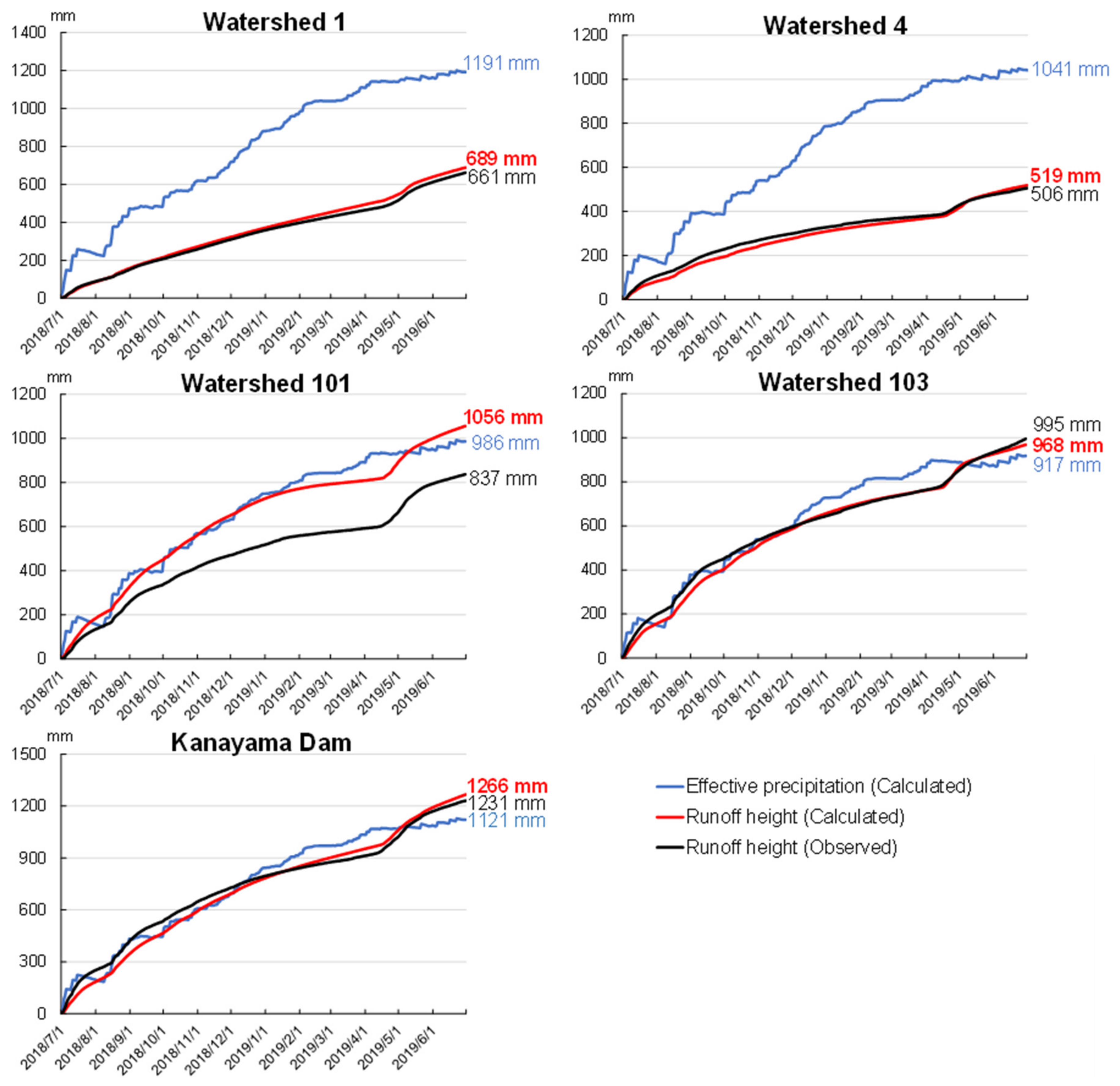
To verify the water balance related to the calculated water volume for each subwatershed and the Kanayama Dam watershed, the cumulative values of the calculated effective precipitation, calculated runoff height, and observed runoff height for one hydrologic year from 1 July 2018 to 30 June 2019 are shown in Figure 7. In the watersheds except for watershed 101, the difference between the cumulative value of the calculated and observed runoff height is less than 5%, indicating that the reproduction is consistent in terms of water balance. In watershed 101, the observed runoff height is 21% smaller than the calculated runoff height. Comparing each of the cumulative values for watershed 101 with those for watershed 103, which shares the same characteristic of being composed of Mesozoic rocks, there are no significant differences in the calculated runoff height or effective precipitation, but the observed runoff height is small. While the observed runoff height is calculated by converting the observed water level into a stream discharge based on the field observation, in watershed 101, the observed outflow may have been under-derived, which could be due to errors in the stream discharge observation or in the conversion from the water level to stream discharge.

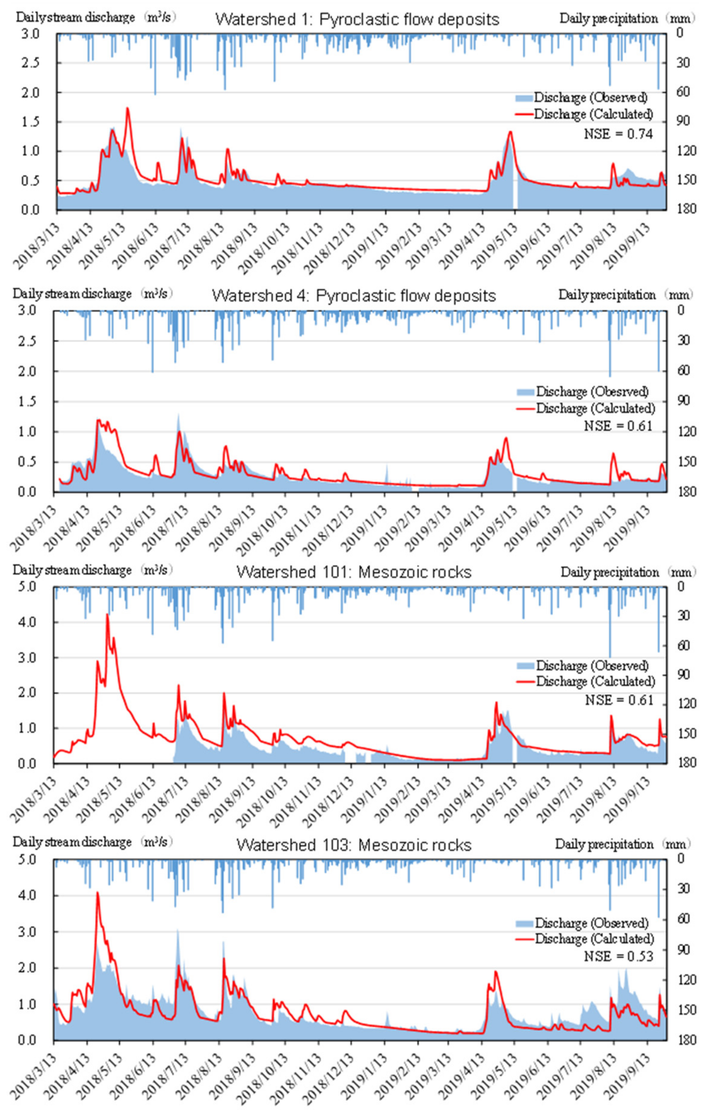
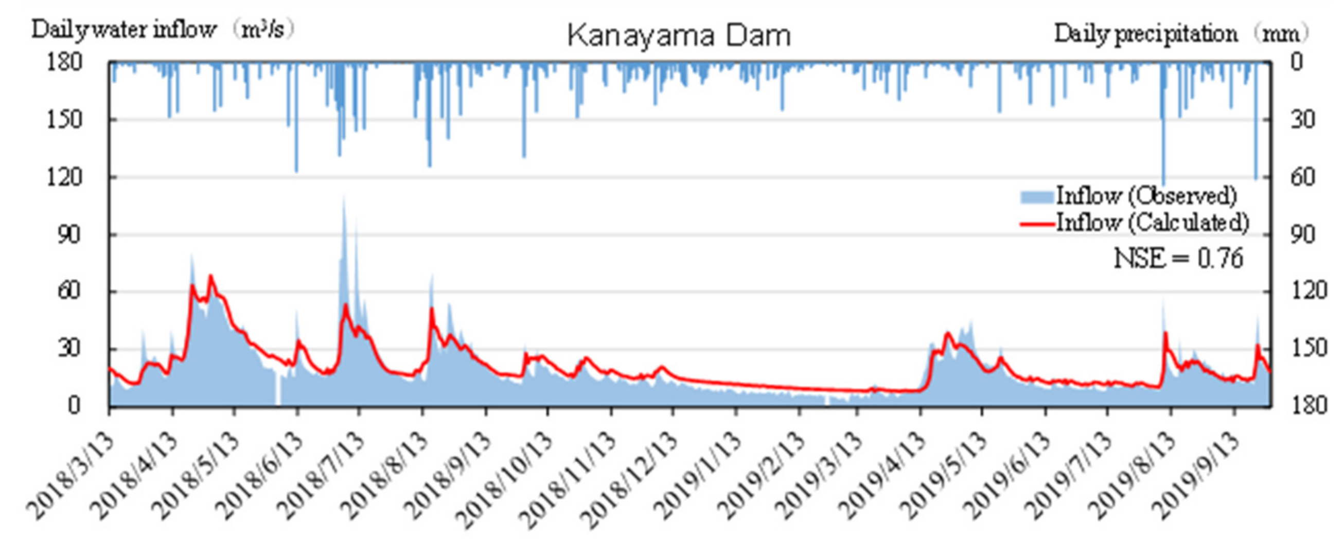
The reproduction results of the discharge in the subwatersheds and the Kanayama Dam watershed are shown in Figure 8 and Figure 9, respectively. The NSEs for the calculated stream discharges for the four subwatersheds ranged from 0.53 to 0.74, while the NSE for the Kanayama Dam Lake was 0.76. These values correspond to good (0.70 < NSE ≤ 0.80) or satisfactory (0.50 < NSE ≤ 0.70) according to Moriasi’s NSE evaluation criteria for daily stream discharge at the watershed scale [55]. This indicates the reproducibility of stream discharge at each site.

3.2. Reproduction of the Water Temperature

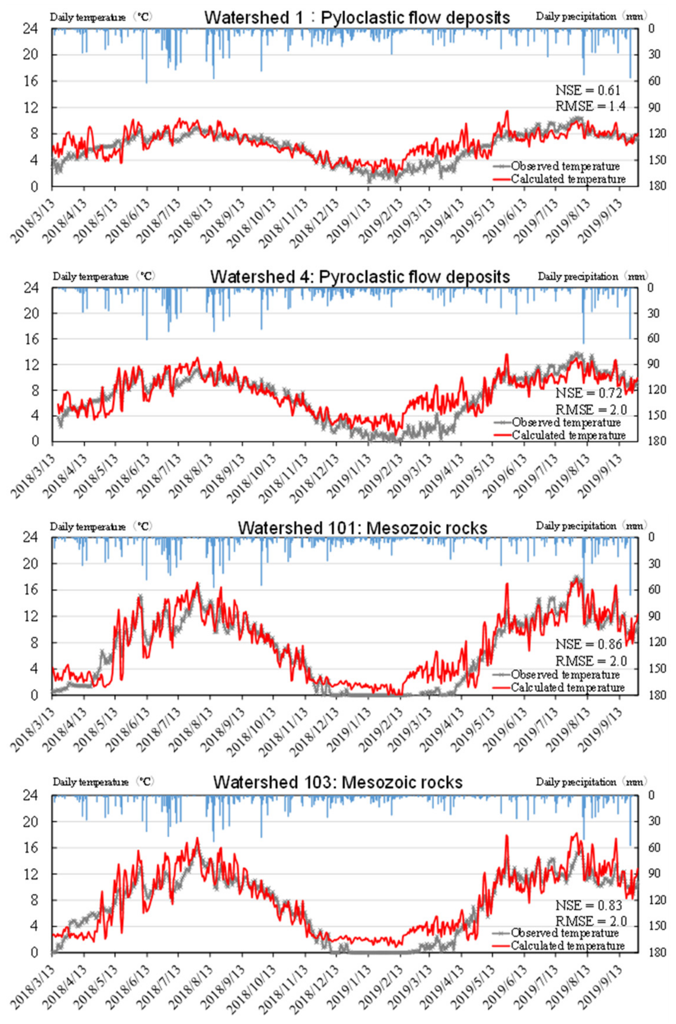
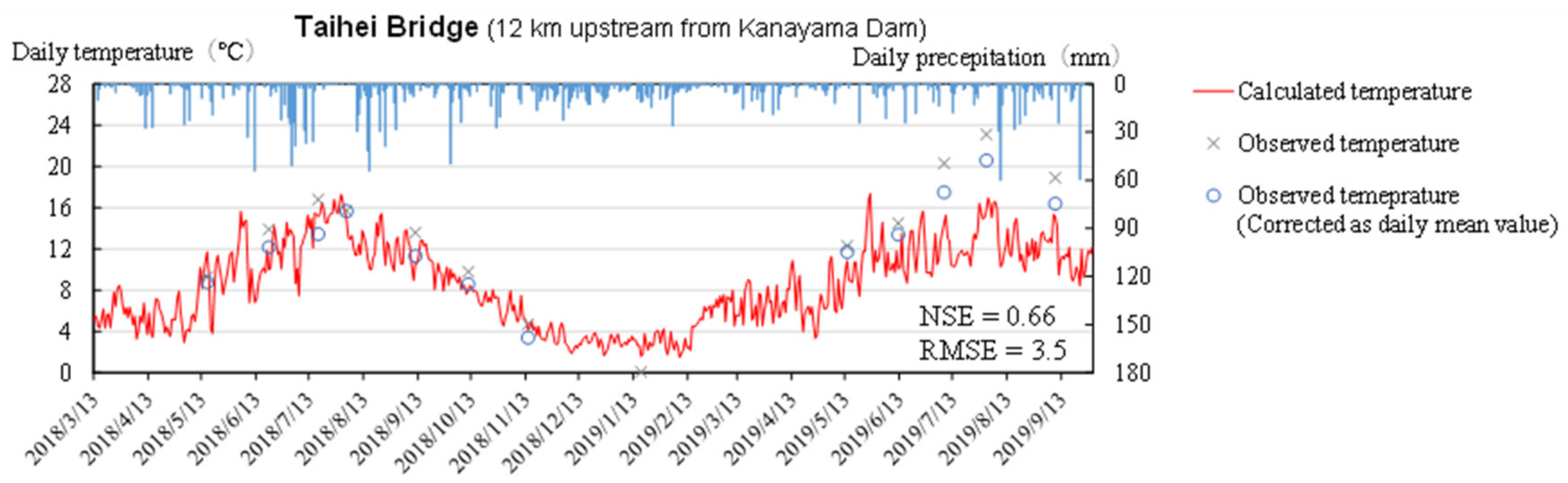
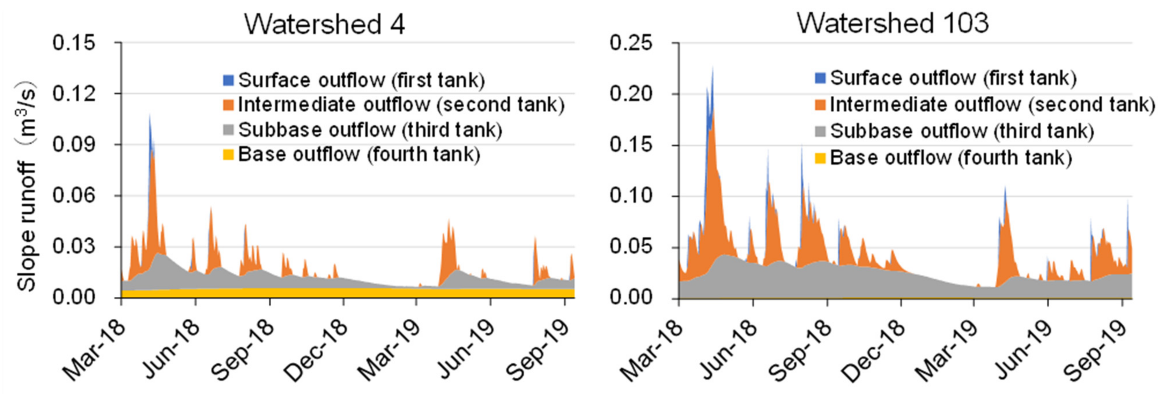
The results of water temperature reproduction in the subwatersheds and the Taihei bridge are shown in Figure 10 and Figure 11, respectively. The NSEs and RMSEs for the calculated water temperatures in watersheds 1, 4, 101, and 103 ranged from 0.61 to 0.86 and 1.4 to 2.0 °C, respectively. The NSE at the Taihei bridge was 0.66, similar to those of the four subwatersheds. Assuming that Moriasi’s criteria for stream discharge on NSE [55] can be similarly applied to water temperature, reasonable reproducibility of water temperature is found at each site. The RMSE of 3.5 °C at the Taihei bridge was larger than that in watersheds 1, 4, 101, and 103, possibly due to the limited number of water temperature observations at the Taihei bridge and the inclusion of data with discrepancies between the observed and calculated values in the summer of 2019. Comparing the characteristics of the water temperature between the watersheds with pyroclastic flow deposits and with Mesozoic rocks, the watersheds with pyroclastic flow deposits have lower temperatures in summer and higher temperatures in winter, and the difference in the water temperature between the summer and winter is smaller (Figure 10). As shown in Figure 12, the cause of this is that in the watersheds with pyroclastic flow deposits, the ratios of base runoff with more stable water temperature are higher than those in the watersheds with Mesozoic rocks, while the ratios of the surface outflow and the intermediate outflow with high water temperature fluctuations are relatively small.

3.3. Simulated Future Water Temperature

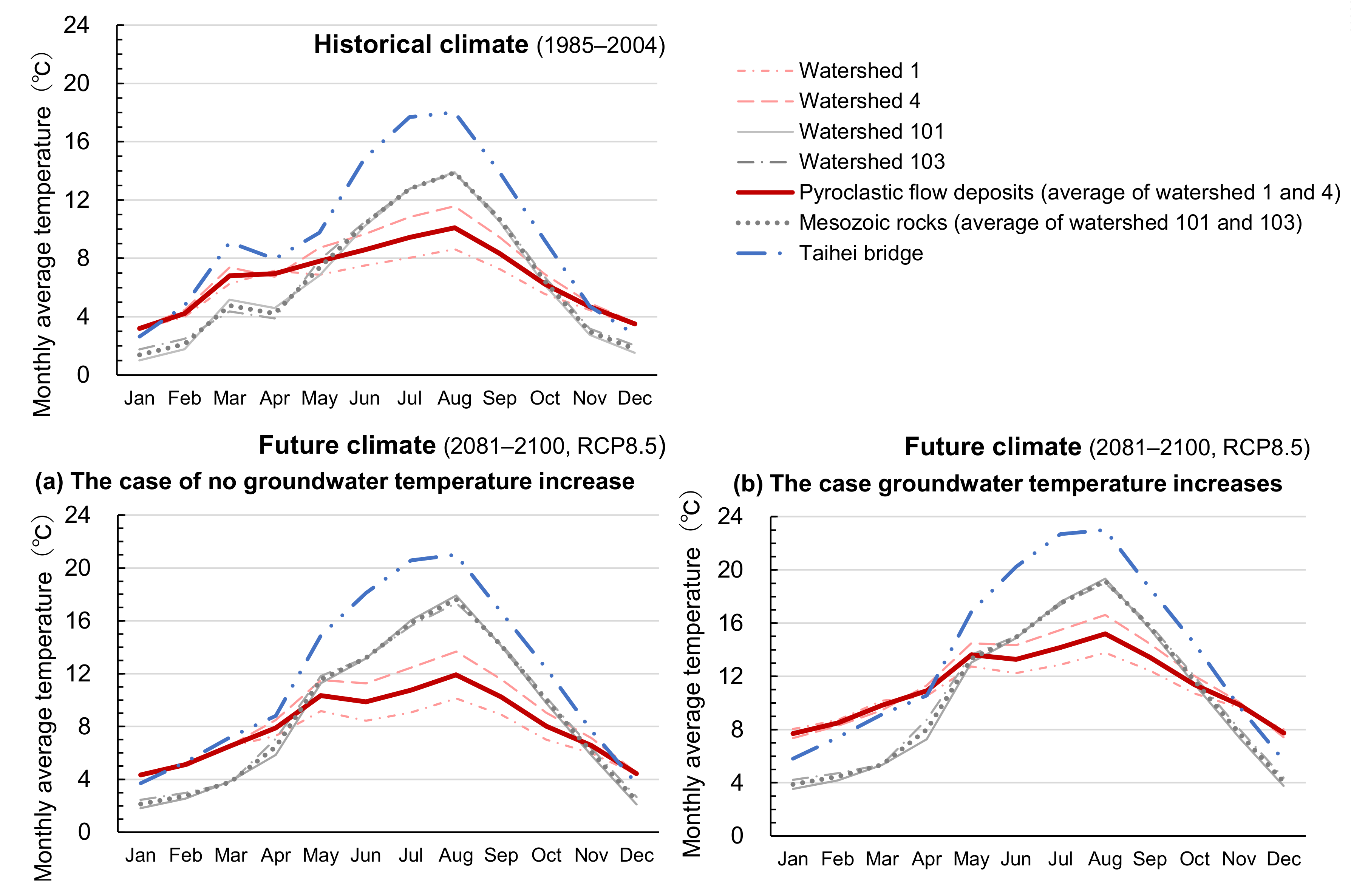
The stream water temperatures under the historical and future climates at four subwatersheds are shown in Figure 13, and the average amounts of water temperature rise between the historical and future climates are shown in Figure 14 by month. Cases where the future groundwater temperature or the base outflow water temperature ${\mathsf{\phi }}_{4\mathrm{i}}$ do not change from the historical climate are shown in (a), and cases where it is assumed to increase by the same amount as the air temperature increase during the same period are shown in (b). In both (a) and (b), the accuracy of reproducing the current situation is slightly inferior in terms of the water temperature during the snowy season, implying that relatively high errors may occur in future forecasts in the snowy season.

Figure 13 shows that in both cases (a) and (b), the annual water temperature fluctuation is relatively small in the watersheds with pyroclastic flow deposits, and the summer water temperature remains lower than that in the watersheds with Mesozoic rocks.

Figure 14 shows that, assuming no increase in the groundwater temperature in (a), the average annual increase in the water temperature in the watersheds with pyroclastic flow deposits is only 1.4 °C per year, while in (b), the average annual increase is 4.6 °C. Compared with the increase in the water temperature in the watersheds with Mesozoic rocks (a: 2.5 °C increase, b: 3.9 °C increase), the increase is slightly smaller in (a) and the same level or slightly larger in (b). This indicates that the effect of mitigation by groundwater on the rise in water temperature in the pyroclastic flow deposits varies considerably depending on whether the rise in groundwater temperature is accompanied by a rise in air temperature, and this effect becomes weaker when the groundwater temperature rise is high.

As for trends at the Taihei bridge site, it is predicted that the water temperature will be higher in both cases (a) and (b) from Figure 13 than in the watersheds with pyroclastic flow deposits and those with Mesozoic rocks. The amount of water temperature rise for the Taihei bridge site is similar to those of the watersheds with Mesozoic rocks in Figure 14 according to the annual average.

4. Discussion

The model developed in this study reproduced the present-day variability characteristics of stream discharge and water temperature well (Figure 8, Figure 9, Figure 10 and Figure 11) according to different geological conditions, as well as the water balance for each watershed (Figure 7). The results demonstrated that the relatively newer pyroclastic flow deposit areas, which are more dependent on groundwater runoff, have smaller annual fluctuations in the water temperature. This result is consistent with the findings of Tague et al. [17] and Ishiyama et al. [19] that geologic features that contribute to groundwater discharge and those with high drought-specific flow suppress maximum summer water temperatures.

Although there is a considerable range in the predicted values depending on how future changes in the groundwater temperature are predicted, this study shows that streams with geologic characteristics that are strongly influenced by groundwater will have smaller annual water temperature fluctuations and more suppressed summer water temperatures in the future climate compared with streams with less groundwater influence.

Ishiyama et al. [19] suggested that the response of the summer water temperature to future climate change depends on the type of geology in the watershed based on empirical statistical relationships among variables, including the geology, summer temperature, and precipitation. This method cannot accurately account for the effects of changes in snow accumulation and snowmelt and changes in the groundwater recharge and runoff due to climate change if past relationships do not hold in the future. The model in this study, although it still partly relies on empirical rules such as the assumption of groundwater runoff temperature, is based on predicting changes in snow accumulation and snowmelt, and changes in the groundwater recharge and runoff. As a result, the primary conclusion that future summer water temperatures in RCP 8.5 are expected to increase substantially for both pyroclastic flow deposits and Mesozoic distribution areas, but that future water temperatures in pyroclastic flow distribution areas will remain lower than those in the Mesozoic distribution areas, is consistent with Ishiyama et al. [19]. This study provides a more solid physical basis for the future trends in water temperature increase proposed by Ishiyama et al. In addition, Ishiyama et al. [19] only covered the summer season, whereas this study provides new information on future projections for the entire year. This study highlights that water temperatures overall are higher in the pyroclastic flow deposit distribution areas than in the Mesozoic distribution areas in winter.

Several previous studies have predicted the discharge and water temperature of streams in snowy cold regions [7,8,10,20] using physics-based models that take snow accumulation processes into account, but these studies did not focus on differences in the behavior of water temperature depending on the geological conditions. Leach and Moore [20] used a sensitivity analysis approach with a physics-based model to examine the extent to which future water temperature increases vary with the magnitude of the groundwater contribution to stream flow, but they did not directly address differences in the water temperature response due to geologic factors. This is the first study to demonstrate the differences in the future behavior of water temperature depending on the geological conditions in a region using a physics-based model.

The findings of this study on future changes in the stream water temperatures in different geological conditions under climate change will be useful in considering conservation measures for stream ecosystems, including the consideration of streams that should be prioritized for the conservation for cold-water fish [19]. The results of this study indicate that pyroclastic flow distribution areas are more likely to avoid high summer water temperatures than Mesozoic distribution areas (Figure 13). This may be advantageous for the survival of cold-water fish, which are known to be vulnerable to high summer water temperatures. It is expected that the model prediction results of this study will enable a close examination of appropriate refuge sites. Future predictions of water temperature in the area are also expected to be used in basic research related to the future conservation of stream ecosystems, such as modeling the gene flow, which could be an indicator of connectivity among riverine populations [56].

Among the various hydrologic processes examined, it is difficult to make rigorous assumptions about the increase in the groundwater temperature associated with future increases in the air temperature. The results of this study (Figure 14) confirm that the effect of groundwater mitigation on the water temperature increases in the pyroclastic flow distribution area significantly differs between when groundwater temperature is and is not assumed to increase with air temperature, with the increase in air temperature showing a weaker effect. This is consistent with Leach and Moore [20], who found that future projected increases in stream temperature vary considerably depending on how future changes in the groundwater temperature are assumed. How groundwater temperature responds to climate warming needs to be further investigated, as it will greatly affect the range of water temperature increases and may be key to a more detailed assessment of the effects of climate change on stream ecosystems.

References

- Michel, A.; Brauchli, T.; Lehning, M.; Schaefli, B.; Huwald, H. Stream temperature and discharge evolution in Switzerland over the last 50 years: Annual and seasonal behaviour. Hydrol. Earth Syst. Sci. 2020, 24, 115–142. [Google Scholar] [CrossRef] [Green Version]
- Webb, B.W.; Nobilis, F. Long-term changes in river temperature and the influence of climatic and hydrological factors. Hydrol. Sci. J. 2007, 52, 74–85. [Google Scholar] [CrossRef]
- Orr, H.G.; Simpson, G.L.; des Clers, S.; Watts, G.; Hughes, M.; Hannaford, J.; Dunbar, M.J.; Laizé, C.L.R.; Wilby, R.L.; Battarbee, R.W.; et al. Detecting changing river temperatures in England and Wales. Hydrol. Process. 2015, 29, 752–766. [Google Scholar] [CrossRef] [Green Version]
- Isaak, D.J.; Wollrab, S.; Horan, D.; Chandler, G. Climate change effects on stream and river temperatures across the northwest U.S. from 1980–2009 and implications for salmonid fishes. Clim. Chang. 2012, 113, 499–524. [Google Scholar] [CrossRef] [Green Version]
- Yao, Y.; Tian, H.; Kalin, L.; Pan, S.; Friedrichs, M.A.M.; Wang, J.; Li, Y. Contrasting stream water temperature responses to global change in the Mid-Atlantic Region of the United States: A process-based modeling study. J. Hydrol. 2021, 601, 126633. [Google Scholar] [CrossRef]
- Van Vliet, M.T.H.; Franssen, W.H.P.; Yearsley, J.R.; Ludwig, F.; Haddeland, I.; Lettenmaier, D.P.; Kabat, P. Global river discharge and water temperature under climate change. Glob. Environ. Change 2013, 23, 450–464. [Google Scholar] [CrossRef]
- Kudo, K.; Nakatsugawa, M.; Chida, Y. Research on evaluation of the water temperature change in snowy cold river based on global warming scenarios. J. Jpn. Soc. Civ. Ser. B1 2018, 74, I_37–I_42. [Google Scholar] [CrossRef]
- Michel, A.; Schaefli, B.; Wever, N.; Zekollari, H.; Lehning, M.; Huwald, H. Future water temperature of rivers in Switzerland under climate change investigated with physics-based models. Hydrol. Earth Syst. Sci. 2022, 26, 1063–1087. [Google Scholar] [CrossRef]
- Ficklin, D.L.; Barnhart, B.L.; Knouft, J.H.; Stewart, I.T.; Maurer, E.P.; Letsinger, S.L.; Whittaker, G.W. Climate change and stream temperature projections in the Columbia River basin: Habitat implications of spatial variation in hydrologic drivers. Hydrol. Earth Syst. Sci. 2014, 18, 4897–4912. [Google Scholar] [CrossRef] [Green Version]
- Lee, S.-Y.; Fullerton, A.H.; Sun, N.; Torgersen, C.E. Projecting spatiotemporally explicit effects of climate change on stream temperature: A model comparison and implications for coldwater fishes. J. Hydrol. 2020, 588, 125066. [Google Scholar] [CrossRef]
- Leach, J.A.; Moore, R.D. Winter stream temperature in the rain-on-snow zone of the Pacific Northwest: Influences of hillslope runoff and transient snow cover. Hydrol. Earth Syst. Sci. 2014, 18, 819–838. [Google Scholar] [CrossRef] [Green Version]
- Ducharne, A. Importance of stream temperature to climate change impact on water quality. Hydrol. Earth Syst. Sci. 2008, 12, 797–810. [Google Scholar] [CrossRef] [Green Version]
- Förster, H.; Lilliestam, J. Modeling thermoelectric power generation in view of climate change. Reg. Environ. Change 2009, 10, 327–338. [Google Scholar] [CrossRef]
- Fullerton, A.H.; Torgersen, C.E.; Lawler, J.J.; Steel, E.A.; Ebersole, J.L.; Lee, S.Y. Longitudinal thermal heterogeneity in rivers and refugia for coldwater species: Effects of scale and climate change. Aquat. Sci. 2018, 80, 3. [Google Scholar] [CrossRef]
- Isaak, D.J.; Young, M.K.; Nagel, D.E.; Horan, D.L.; Groce, M.C. The cold-water climate shield: Delineating refugia for preserving salmonid fishes through the 21st century. Glob. Change Biol. 2015, 21, 2540–2553. [Google Scholar] [CrossRef]
- Caissie, D. The thermal regime of rivers: A review. Freshw. Biol. 2006, 51, 1389–1406. [Google Scholar] [CrossRef]
- Tague, C.; Farrell, M.; Grant, G.; Lewis, S.; Rey, S. Hydrogeologic controls on summer stream temperatures in the McKenzie River basin, Oregon. Hydrol. Process. 2007, 21, 3288–3300. [Google Scholar] [CrossRef]
- Nagasaka, A.; Sugiyama, S. Factors affecting the summer maximum stream temperature of small streams in northern Japan. Bull. Hokkaido For. Res. Inst. 2010, 47, 35–43. [Google Scholar]
- Ishiyama, N.; Sueyoshi, M.; Molinos, J.G.; Iwasaki, K.; Negishi, J.N.; Koizumi, I.; Nagayama, S.; Nakamura, F. The role of geology in creating stream climate-change refugia along climate gradients. bioRxiv 2022. bioRxiv:2022.2005.2002.490355. [Google Scholar] [CrossRef]
- Leach, J.A.; Moore, R.D. Empirical stream thermal sensitivities may underestimate stream temperature response to climate warming. Water Resour. Res. 2019, 55, 5453–5467. [Google Scholar] [CrossRef]
- Ministry of Land, Infrastructure, Transport and Tourism Hokkaido Development Bureau. River Maintenance Plan of Sorachi River, Ishikari River System (Modified Version); Ministry of Land, Infrastructure, Transport and Tourism: Tokyo, Japan, 2018.
- The Geological Survey of Hokkaido, Industrial Promotion Department of Kamikawa Branch Office. Geology and Underground Resources of Kamikawa Branch Office, Ⅰ Southern Part of Kamikawa Region; Geological Survey of Hokkaido: Sapporo, Japan, 2008; p. 45. [Google Scholar]
- Sapporo Regional Headquarters, Japan Meteorological Agency. Climatic Change in Hokkaido, 2nd ed.; Sapporo Regional Headquarters, Japan Meteorological Agency: Sapporo, Japan, 2017.
- Usutani, T.; Nakastugawa, M.; Matsuoka, N. Generalization of model parameters for evaluating basin-scale soil moisture content. J. Jpn. Soc. Civ. Ser. B1 2014, 70, I_355–I_360. [Google Scholar] [CrossRef] [Green Version]
- Musiake, K.; Takahasi, Y.; Ando, Y. Effects of basin geology on river-flow regime in mountainous areas of Japan. Nat. Commun. 1981, 1981, 51–62. [Google Scholar] [CrossRef]
- Ministry of Land, Infrastructure, Transport and Tourism. Water Information System. Available online: http://www1.river.go.jp/ (accessed on 10 February 2022).
- Japan Meteorological Agency. Historical Weather Data Search. Available online: http://www.data.jma.go.jp/obd/stats/etrn/index.php (accessed on 10 February 2022).
- Ueda, S.; Nakatsugawa, M.; Usutani, T. Estimation of high-resolution downscaled climate information based on verification of water balance in watershed of Hokkaido. J. Jpn. Soc. Civ. Ser. B1 2020, 76, I_25–I_30. [Google Scholar] [CrossRef]
- Sasaki, H.; Murata, A.; Kawase, H.; Hanafusa, M.; Nosaka, M.; Oh’izumi, M.; Mizuta, R.; Aoyagi, T.; Shido, F.; Ishihara, K. Projection of future climate change around Japan by using MRI non-hydrostatic regional climate model. Tech. Rep. Meteorol. Res. Inst. 2015, 73, 1–90. [Google Scholar] [CrossRef]
- IPCC. Climate Change 2014: Synthesis Report. In Contribution of Working Groups I, II and III to the Fifth Assessment Report of the Intergovernmental Panel on Climate Change; Core Writing Team, Pachauri, R.K., Meyer, L.A., Eds.; IPCC: Geneva, Switzerland, 2014; p. 151. [Google Scholar]
- Mizuta, R.; Arakawa, O.; Ose, T.; Kusunoki, S.; Endo, H.; Kitoh, A. Classification of CMIP5 future climate responses by the tropical sea surface temperature changes. SOLA 2014, 10, 167–171. [Google Scholar] [CrossRef] [Green Version]
- Ueda, S.; Nakatsugawa, M.; Chida, Y.; Komatsu, A. Production of downscaled data for Hokkaido which basin water balance has been verified. J. Jpn. Soc. Civ. Ser. B1 2019, 75, I_1051–I_1056. [Google Scholar] [CrossRef]
- Usutani, T.; Nakatusgawa, M.; Kudo, K. Quantitative analysis of hydrologic process in the Ishikari river catchment area. J. Jpn. Soc. Civ. Ser. B1 2005, 49, 229–234. [Google Scholar] [CrossRef] [Green Version]
- Kondo, J. Meteorology of Water Environment; Asakura Publishing: Tokyo, Japan, 1994. [Google Scholar]
- Kuchizawa, H.; Nakatsugawa, M. Estimations of snow pack condition and evapotranspiration based on water and heat balances in watersheds. Mon. Rep. Civ. Eng. Res. Inst. Hokkaido 2002, 588, 19–38. [Google Scholar]
- Nakatsugawa, M.; Hamahara, Y.; Hoshi, K. Long-term runoff calculation considering change of snow pack condition. J. Hydrosci. Hydraul. Eng. 2004, 22, 155–169. [Google Scholar] [CrossRef] [Green Version]
- Foundation of Hokkaido River Disaster Prevention Research Center. Ishikari River Basin Landscape Information; Foundation of Hokkaido River Disaster Prevention Research Center: Sapporo, Japan, 1998. [Google Scholar]
- Sugawara, M. Automatic calibration of the tank model. Hydrol. Sci. Bull. 1979, 24, 375–388. [Google Scholar] [CrossRef]
- Duan, Q.; Sorooshian, S.; Gupta, V. Effective and efficient global optimization for conceptual rainfall-runoff models. Water Resour. Res. 1992, 28, 1015–1031. [Google Scholar] [CrossRef]
- Tanakamaru, H. Parameter estimation for the tank model using global optimization. Trans. Jpn. Soc. Irrig. Drain. Reclam. Eng. 1995, 1995, 503–512. [Google Scholar] [CrossRef]
- Leopold, L.B.; Maddock, T., Jr. The Hydraulic Geometry of Stream Channels and Some Physiographic Implications; USGS Professional Paper, 252; US Government Printing Office: Washington, DC, USA, 1953; p. 57.
- Arai, T.; Nishizawa, T. Water Temperature; Kyoritu Publishing Company: Tokyo, Japan, 1974; Volume 10. [Google Scholar]
- Strahler, A.N. Hypsometric (area-altitude) analysis of erosional topography. Geol. Soc. Am. Bull. 1952, 63, 1117–1142. [Google Scholar] [CrossRef]
- Google Earth. Available online: https://www.google.co.jp/intl/ja/earth/ (accessed on 14 December 2021).
- Nash, J.E.; Sutcliffe, J.V. River flow forecasting through conceptual models part I—A discussion of principles. J. Hydrol. 1970, 10, 282–290. [Google Scholar] [CrossRef]
- Arai, T. Climate change and variations in the water temperature and ice cover of inland waters. Jpn. J. Limnnol. 2009, 70, 99–116. [Google Scholar] [CrossRef] [Green Version]
- Menberg, K.; Blum, P.; Kurylyk, B.L.; Bayer, P. Observed groundwater temperature response to recent climate change. Hydrol. Earth Syst. Sci. 2014, 18, 4453–4466. [Google Scholar] [CrossRef] [Green Version]
- Figura, S.; Livingstone, D.M.; Hoehn, E.; Kipfer, R. Regime shift in groundwater temperature triggered by the Arctic Oscillation. Geophys. Res. Lett. 2011, 38, L23401. [Google Scholar] [CrossRef] [Green Version]
- Hemmerle, H.; Bayer, P. Climate change yields groundwater warming in Bavaria, Germany. Front. Earth Sci. 2020, 8, 523. [Google Scholar] [CrossRef]
- Burns, E.R.; Zhu, Y.; Zhan, H.; Manga, M.; Williams, C.F.; Ingebritsen, S.E.; Dunham, J.B. Thermal effect of climate change on groundwater-fed ecosystems. Water Resour. Res. 2017, 53, 3341–3351. [Google Scholar] [CrossRef]
- Matsuyama, H.; Miyano, H. Diagnostic study on warming mechanism of spring water temperature based on field observations and numerical simulation: A case study of Masugatanoike spring, Tokyo, Japan. Hydrol. Res. Lett. 2011, 5, 78–82. [Google Scholar] [CrossRef] [Green Version]
- Yamazaki, T.; Taguchi, B.; Kondo, J. Estimation of the heat balance in a small snow-covered forested catchment basin. Tenki 1994, 41, 71–77. [Google Scholar]
- Ishii, T.; Nashimoto, M.; Shimogaki, H. Estimation of leaf area index using remote sensing data. J. Jpn. Soc. Hydrol. Water Res. 1999, 12, 210–220. [Google Scholar] [CrossRef] [Green Version]
- Tokuda, D.; Yamazaki, D.; Oki, T. Study of the role of inundation on river water temperature with a numerical model. J. Jpn. Soc. Civ. Ser. B1 2017, 73, I_1213–I_1218. [Google Scholar] [CrossRef] [Green Version]
- Moriasi, D.; Gitau, M.; Pai, N.; Daggupati, P. Hydrologic and water quality models: Performance measures and evaluation criteria. Trans. ASABE 2015, 58, 1763–1785. [Google Scholar] [CrossRef] [Green Version]
- Nakajima, S.; Sueyoshi, M.; Hirota, S.K.; Ishiyama, N.; Matsuo, A.; Suyama, Y.; Nakamura, F. A strategic sampling design revealed the local genetic structure of cold-water fluvial sculpin: A focus on groundwater-dependent water temperature heterogeneity. Heredity 2021, 127, 413–422. [Google Scholar] [CrossRef]
Figure 3.
Schematic diagram of the water circulation and water temperature estimation model.
Figure 6.
Conceptual diagram of the water temperature calculation.
Figure 7.
Comparison of the calculated effective precipitation, calculated runoff heights, and observed runoff heights (cumulatively for one hydrologic year) on current reproduction.
Figure 8.
Reproduction of stream discharge in four subwatersheds.
Figure 9.
Reproduction of the inflow at Kanayama Dam.
Figure 10.
Reproduction of stream temperatures in the four subwatersheds.
Figure 11.
Reproduction of the stream temperature at the Taihei bridge.
Figure 12.
Slope runoff for each component in subwatersheds (left: watershed 4 composed of pyroclastic flow deposits, right: watershed 103 composed of Mesozoic rocks). For watershed 4 and 103, the calculated values are shown for the 1 km mesh where the stream discharge and water temperature observation points are located.
Figure 13.
Estimated stream temperatures for the historical and future climates (RCP 8.5). (a): Stream temperatures assuming that average groundwater temperatures remain the same between the historical and future climates. (b): Stream temperatures assuming that groundwater temperature increases equal to the increase in air temperature.
Figure 14.
Estimated changes in the stream water temperature between the historical and future climates (RCP8.5). Comparisons were made with no increase in the groundwater temperature (assuming that the groundwater temperature was at the same level as the historical climate) and with an increase in the groundwater temperature (assuming that the groundwater temperature increased by the same amount as the annual average air temperature). The dotted line shows the annual average increase in the water temperature.