Numerical Investigation of the Scaling Effects for a Point Absorber

Abstract

In order to design and evaluate the behaviour of a numerically optimised wave energy converter (WEC), a recommended procedure is to initially study small scale models in controlled laboratory conditions and then progress further up until the full-scale is reached. At any point, an important step is the correct selection of the wave theory to model the dynamical behaviour of the WEC. Most authors recommend the selection of a wave theory based on dimensional parameters, which usually does not consider the model scale. In this work, the scale effects for a point absorber are studied based on numerical simulations for three different regular waves conditions. Furthermore, three different wave theories are used to simulate two scales 1:1 and 1:50. The WEC-wave interaction is modelled by using a numerical wave tank implemented in ANSYS-Fluent with a floating object representing the WEC. Results show that the normalised difference between 1:1 and 1:50 models, keeping the same wave theory fluctuate between 30% and 58% of the WEC heave motion and that a wrong selection of the wave theory can lead to differences up to 138% for the same variable. It is also found that the limits for the use of wave theories depends on the particular model and that the range of applicability of different theories can be extended.

1. Introduction

Wave Energy Converter

The potential to generate clean and renewable energy from the ocean has long been recognised [1] and has been estimated to be capable of providing 32,000 TWh/yr globally [2]. Nevertheless, this technology is still relatively immature [3] and Wave Energy Converter (WEC) device development is ongoing.

The hydrodynamic development and optimisation of WECs is typically achieved through a combination of physical (i.e., in the laboratory) and numerical modelling. Numerical approaches operating in the time and/or frequency domain [4] include mesh based solvers [5,6] and Smoothed-particle hydrodynamics (SPH) [7,8]. Numerical modelling is especially useful for the investigation of interaction of multiple devices [9,10,11], but requires specific validation data provided by nature or laboratory experimental investigations. Novel WECs are commonly tested and optimised under laboratory conditions. This staged development procedure starts with small scale models in controlled laboratory conditions before moving to larger scale sea trials [3,12]. This staged approach has been adopted in the latest international standards [13] to provide a development pathway with research and development processes appropriate to the Technology Readiness Level (TRL) of the project. Understanding the uncertainties in the laboratory is key to understanding the significance of the measured data and results [14,15]. Small scale hydrodynamic model tests are usually performed according to Froude’s scaling law [16,17]. Froude similarity ensures that the correct relationship is maintained between inertial and gravitational forces when the full-scale object is scaled down to model dimensions, and is therefore appropriate for model tests involving water waves. Applying this to WEC development, if the Reynolds numbers for two geometrically similar floating objects are large enough, then the viscous terms in the non-dimensional Navier–Stokes equation can be neglected. However, at small Reynolds numbers, the viscous effects could become relevant. Shen et al. [12] recommend Reynolds numbers higher than 10⁵ in order to neglect the viscous effects for all type of wave energy converters. Nevertheless, scale effects have been studied separately for different types of WECs with varying results. Schmitt and Elsaber [18] give a detailed discussion on the suitability of Froude scaling laws for a Oscillating Wave Surge Converter (OWSC) where they numerically test its behaviour by scaling the fluid viscosity. In this study they conclude that the differences in flow patterns for different scales can be explained by the changes in viscosity, nevertheless they state that some uncertainties remain related to the mesh influence. Palm et al. [19] analyse the nonlinear forces on a moored point absorber wave energy converter (PA-WEC) at prototype and model scale using CFD for two wave conditions, finding an amplitude response reduction between 1 and 4% due to viscous forces and between 18 and 19% due to induced drag, non-linear added mass, and radiation forces. This study was made for two regular 5th order waves in stationary state. Recently, Windt et al. [20,21] studied firstly the scale effect of a moored PA-WEC device exposed to focused waves, finding differences around 5% between different scales, and secondly they studied the hydrodynamic scaling effects for the wavestar WEC exposed to regular and irregular stationary waves, showing that significant scaling effects occur for the viscous component of the hydrodynamic loads on the WEC hull, stating that additional studies are required for extreme events, e.g., breaking waves. In the other hand, in order to simulate trains of regular waves, most authors recommend the selection of a wave theory based on dimensional parameters, where two of the most cited works are from Le Méhauté in 1976 and Hedges in 1995 [22,23]. Based on these recommendations, several authors propose numerical models using, from linear theory [24,25,26,27] to higher order wave theories [28,29], to simulate the wave behaviour. In some of these studies the goal was to numerically model scaled WEC devices where the same wave theory selection map from Le Méhauté was used without considering the influence of the scale effect on the correct selection of the wave theory [26,27]. Hence, the main goal of the presented work is to study the scale effect related to a one DOF point absorber subjected to three different waves and to study how the wave theory applied to these waves influences the predicted WEC behaviour by using different scales. Section 2 provides the theoretical background, which is used for the numerical model presented in Section 3. The gained results are discussed in Section 4 followed by the conclusions in Section 5.

2. Wave Theories

As mentioned, an important step on the WEC modelling process is the correct selection of the wave theory according to the wave characteristics. The most common wave theories used are 1st order Airy theory and 2nd to 5th order Stokes theories. These theories are introduced in this section.

2.1. Airy Wave Theory

Linear Wave theory (LWT) was developed by Airy [30] in 1845 and provides a reasonable description of wave motion in all water depths. This theory relies on the assumption that the wave amplitude A is small in comparison to the wavelength $\lambda$ and therefore higher order terms can be ignored. This allows the simplification that the free surface boundary condition can be linearised. The 2D wave profile $\zeta$ for a linear wave is given by Equation (1):

$$\zeta (x,y,t)=Acos\left(\alpha \right),$$

(1)

where x is the coordinate direction in the wave propagation direction, t is the time, and $\alpha$ is defined in Equation (2):

$$\alpha =k_{x}x+k_{y}y-{\omega }_{e}t+ϵ.$$

(2)

The variables $k_x$ and $k_y$ are the wave number ($k=2\pi /\lambda$) component in the wave propagation direction x and the normal y axis, respectively. $ϵ$ is the phase difference and ${\omega }_e$ is the effective wave frequency [31].

2.2. Stokes Wave Theories

For small amplitude wave theory, the wave steepness $H/\lambda$ (H represents the wave height) is assumed to be small and the water depth is considered infinite or high in relation to the wavelength, then the wave is considered to be linear. Finite amplitude waves require a wave steepness value, which is sufficiently high (but always <1), or that the water depth is small relative to the wave height. The theory of linear waves is not valid for such waves. For this reason it becomes necessary to use higher-order models. These higher order theories were first developed by Stokes [32] in 1847.

The non-linear water waves problem is of great importance because, according to the mechanical modelling of this problem, a relationship exists between the potential flow and pressure exerted by water waves. The difficulty of this problem comes not only from the fact that the kinematic and dynamic conditions are non-linear in relation to the velocity potential, but especially because they are applied at an unknown and variable free surface. To overcome this difficulty, Stokes used an approach consisting of perturbations series around the still water level to develop a non-linear theory.

The software ANSYS-Fluent [31] formulates the Stokes wave theories based on the work by Fenton [33]. These wave theories are valid for high steepness finite amplitudes waves operating in intermediate to deep liquid depth range. The generalised expression for 2D wave profiles for higher order Stokes theories (second to fifth order) is given as shown in Equation (3):

$$\zeta (x,y,t)=\frac{1}{k}\sum _{i=1}^n\sum _{j=1}^i{b}_{ij}{\xi }^{i}cos\left(j\alpha \right),$$

(3)

where $\xi$ is defined as $\xi =\pi H/\lambda$, n wave theory index (2 to 5) and $b_{ij}$ are constants shown in Fenton [33]. It is important to mention that previous theories assume that the propagation of disturbances is collinear [33].

Validity Regions

In order to select the wave theory, Le Méhauté [22] proposed regions of validity based on the dimensional parameters $h/g{\tau }^2$ and $H/g{\tau }^2$, where h is the water depth, g the gravitational acceleration, and $\tau$ is the wave period. Several authors consider this map as a reference for their works. Penalba et al. [34] show that the recommended theory for some common wave energy generators are between 2nd and 4th order Stokes theory according to Le Méhauté recommendations. Later in 1995, Hedges [23] proposed other regions of validity of various analytical wave theories in terms of wave steepness and Ursell number ($H{\lambda }^2/h^3$) in regard to the presence of currents. In order to select the wave theory in the area of wave energy converters, various authors [35,36,37,38,39] use the limits recommended by Le Méhauté or Hedges.

In this work, four different regular waves conditions are studied, which are usually recommended to be modelled by 2nd, 3rd, and 4th order wave theories [22]. The goal of the present work is to study the effect of the scale on the behaviour of the different theories (From 2nd to 4th order) on the prediction of the WEC heave motion in a transient state.

3. Numerical Model

In this section, the 3D numerical wave tank is introduced, which was implemented in ANSYS-Fluent (version 2019 R3) to simulate the waves and the WEC dynamics. Firstly, the description of the numerical wave tank is presented, followed by the mesh characteristics (including the mesh study) together with the boundary conditions applied and finally the solver settings.

3.1. Numerical Wave Tank Characteristics

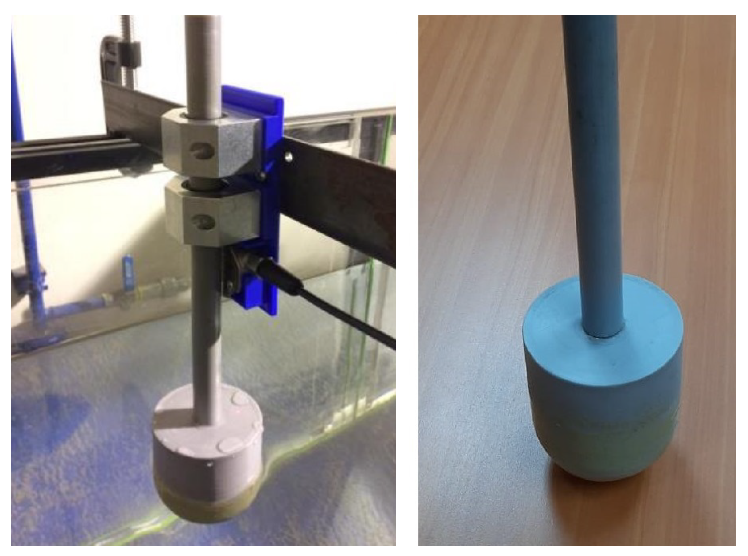
The numerical wave tank used in this study is based on the dimensions of an experimental test rig placed in the Mechanical Engineering department of the Universidad del Bío-Bío. The scale of 1:50 is chosen to be typical for this experimental facility.

Table 1. Dimensions of the tank illustrated in Figure 1 in meters for the different scales.

Scale	h	${\mathit{h}}_{\mathit{m}}$	${\mathit{W}}_{\mathit{t}}$	L	${\mathit{L}}_{\mathit{d}}$	${\mathit{L}}_{\mathit{b}}$	${\mathit{D}}_{\mathit{b}}$	${\mathit{f}}_{\mathit{b}}$
1:1	15	29.58	24	82.0	44.5	3	3.9	1.1695
1:50	0.300	0.5916	0.48	1.64	0.89	0.06	0.078	0.02339

and Figure 1 shows the dimensions of the wave tank and point absorber for scales 1:1 and 1:50 according to Froude similarities [40]. The investigated structure consists of a cylindrical main body with a hemispherical lower surface of diameter $D_b$. The motion response of the buoy was limited to the vertical direction assuming a single point absorbing device. The studied point absorber is shown in Figure 2 and the main characteristics of this device are shown in

Table 2. Characteristics of the studied point absorber at laboratory scale shown in Figure 2.

Parameter	Value	Units
Total mass	0.235	Kg
Construction method	3D printed	-
Material	Polylactic Acid (PLA)	-
Surface treatment	Epoxy adhesive	-
Support method	Axial bearings	-

.

3.2. Solver Settings

The two-phase fluid solver uses the three dimensional incompressible Reynolds-Averaged Navier–Stokes (RANS) equations to express the motion of the two fluids (i.e., water and air). The RANS equations consist of a mass conservation and a momentum conservation equations. In order to represent the two immiscible fluids water and air, the volume of fluid (VOF) model is used.

A numerical beach scheme is applied to the far end of the domain with the aim of reducing the wave reflection. A damping zone of 2 wavelengths long was selected to allow the gradual dissipation of propagating waves. This is completed by adding a sink term, S, to the momentum equation within the specified zone [39]. Additional information on the numerical model is shown in

Table 3. Additional parameters of the numerical wave tank model.

Parameter	Value	Units
Time step	adaptive	s
Turbulence model	realisable $k-ϵ$	-
WEC density	574	kg/m3
Water-Air surface tension	0.074	mN/m

.

3.3. Boundary Conditions

Three different types of waves are studied for the evaluation of the scale effect on the behaviour of the WEC buoy simulated with the different numerical models. These cases are named $w_2$, $w_3$, and $w_4$ based on the order of the targeted Stokes waves. These wave conditions are selected in order to evaluate the recommendation of Le Méhauté [22] for the three different wave theories. The specific settings were also chosen for a future experimental validation of the numerical results in the experimental facility at Universidad del Bío-Bío.

Table 4. Dimensions of the wave for the different scales.

	Scale	Height $\left(\mathit{H}\right)$	Length ($\mathit{\lambda }$)	Period ($\mathit{\tau }$)	$\mathit{h}/\mathit{g}{\mathit{\tau }}^2$	$\mathit{H}/\mathit{g}{\mathit{\tau }}^2$
$w_4$	1:1	4.200 m	30 m	4.394 s	0.0793	0.0222
	1:50	0.084 m	0.6 m	0.621 s	0.0793	0.0222
$w_3$	1:1	2.400 m	30 m	4.394 s	0.0793	0.0127
	1:50	0.048 m	0.6 m	0.621 s	0.0793	0.0127
$w_2$	1:1	1.000 m	30 m	4.394 s	0.0793	0.0053
	1:50	0.020 m	0.6 m	0.621 s	0.0793	0.0053

provides an overview of the input parameters.

ANSYS-Fluent provides the option to simulate the propagation of regular or irregular waves using the boundary condition named open channel wave boundary condition (OCWBC). This boundary condition allows to generate surface gravity waves through velocity inlet boundary conditions by using first order Airy wave theory [30] and higher order Stokes wave theories, among others theories. Thereby, the velocity fields as well as the water level according to the chosen wave theory are calculated and applied at each time step to the secondary phase [31]. The boundary conditions used in this model are summarised in

Table 5. Boundary conditions used in ANSYS-Fluent.

Zone	Boundary Condition
Top	Pressure Outlet
Inlet	Velocity Inlet and OCWBC
Outlet	Pressure Outlet and OCWBC
Walls and buoy	No-slip Wall

.

3.4. Mesh

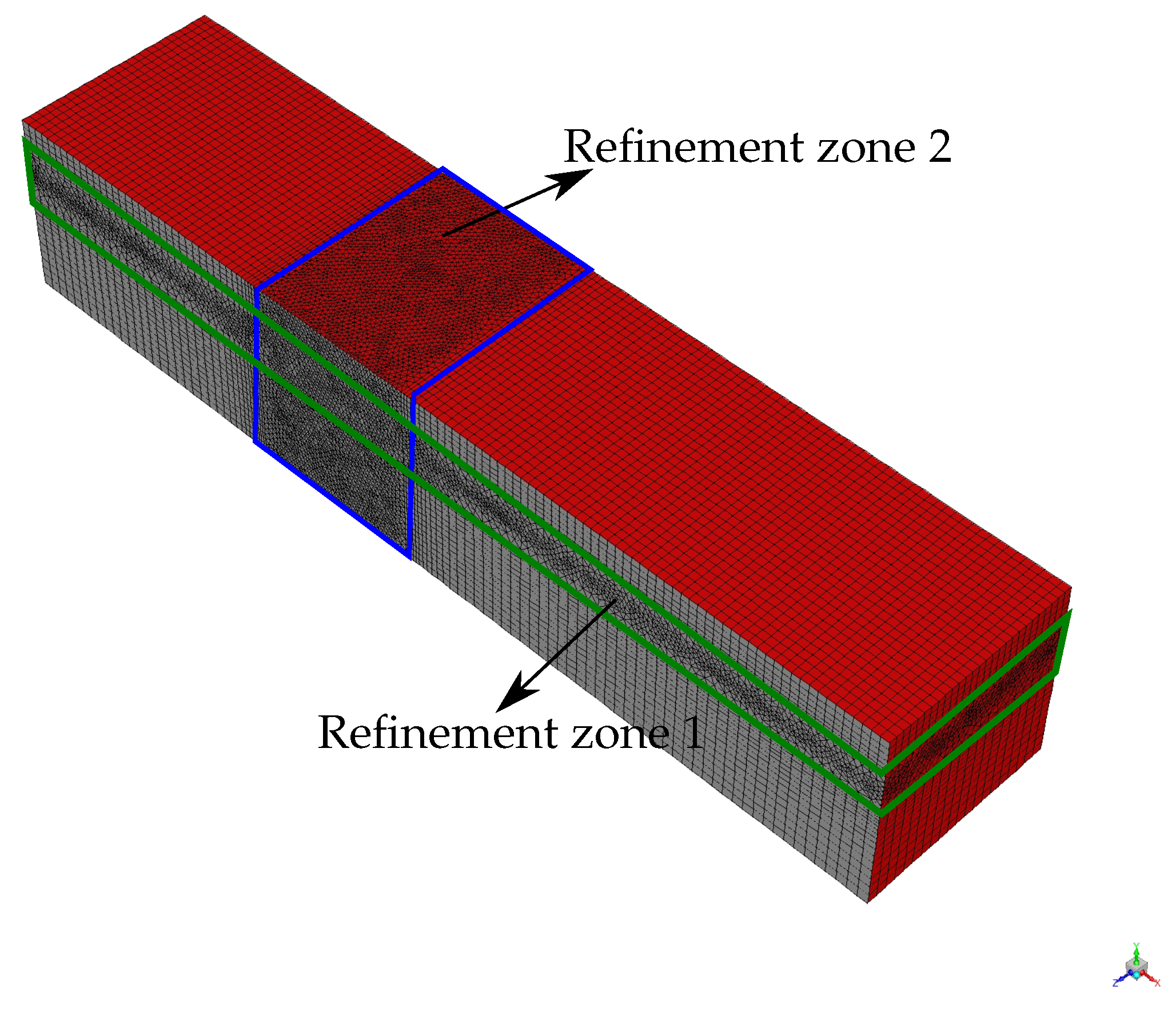
In order to model the free heave movement of the WEC, the six degree of freedom (DOF) solver is used. This model uses the forces and moments of the object to compute the translations and angular motion of the centre of gravity of the object. In this case, the movement is limited to the vertical translation or heave movement and no power take off (PTO) is included. This approach is commonly made for point absorbers [41,42,43]. To create a efficient mesh, two refinement zones are created, the first one in the water-air interface with a thickness of 8 m for the 1:1 case and 0.16 m for the laboratory version. The second one in around the WEC in the cases where this element is included and covers ±1.28$D_b$ in front and after the centre of the buoy. This zones are depicted in Figure 3.

In order to select the correct mesh resolution, the free surface elevation at the middle of the width $W_t$ and at one wavelength from the inlet is studied for three different mesh resolution. This analysis is performed for the following cases:

• Case A: Waves $w_2$, $w_3$, and $w_4$ without WEC, for the scale 1:1 and 1:50;
• Case B: Waves $w_2$, $w_3$, and $w_4$, including the WEC, for the scale 1:1 and 1:50.

The mesh element number divided by the wavelength ($\lambda$) used in each analysis is shown in

Table 6. The mesh element number divided by the wavelength ($\lambda$) case A and B and the two scales, in total zone, refined zone 1 for the case A, and refined zone 1 + refined zone 2 for case B.

N° Ele/$\mathit{\lambda }$	Scale	Mesh 1		Mesh 2		Mesh 3
		Total	Zone 1	Total	Zone 1	Total	Zone 1
Case A	1:1	9758	3955	13,292	5707	3736	23,575
	1:50	350,334	142,026	664,648	285,439	2,007,075	1,270,300
		Total	Zone 1 + 2	Total	Zone 1 + 2	Total	Zone 1 + 2
Case B	1:1	14,265	10,613	17,001	14,445	34,560	27,661
	1:50	715,819	532,584	1,284,762	1,025,800	1,434,264	1,148,041

. This number is shown in the total zone and in the refined zone 1 for the case A and refined zone 1 + refined zone 2, for case B.

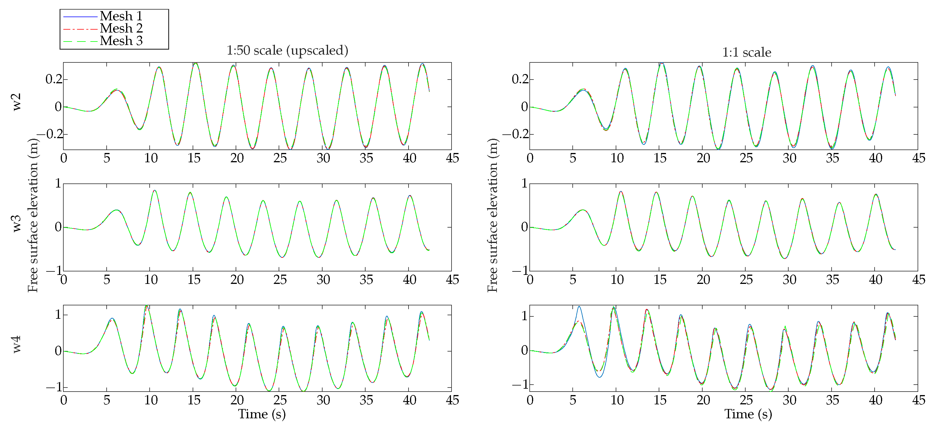
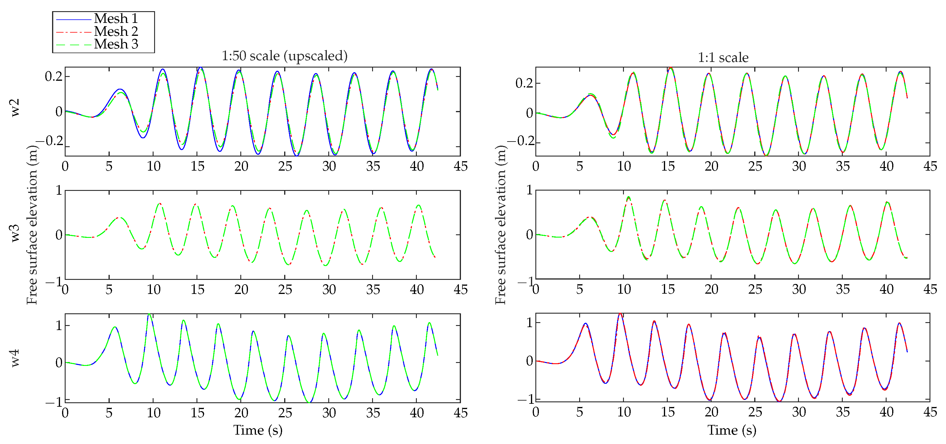
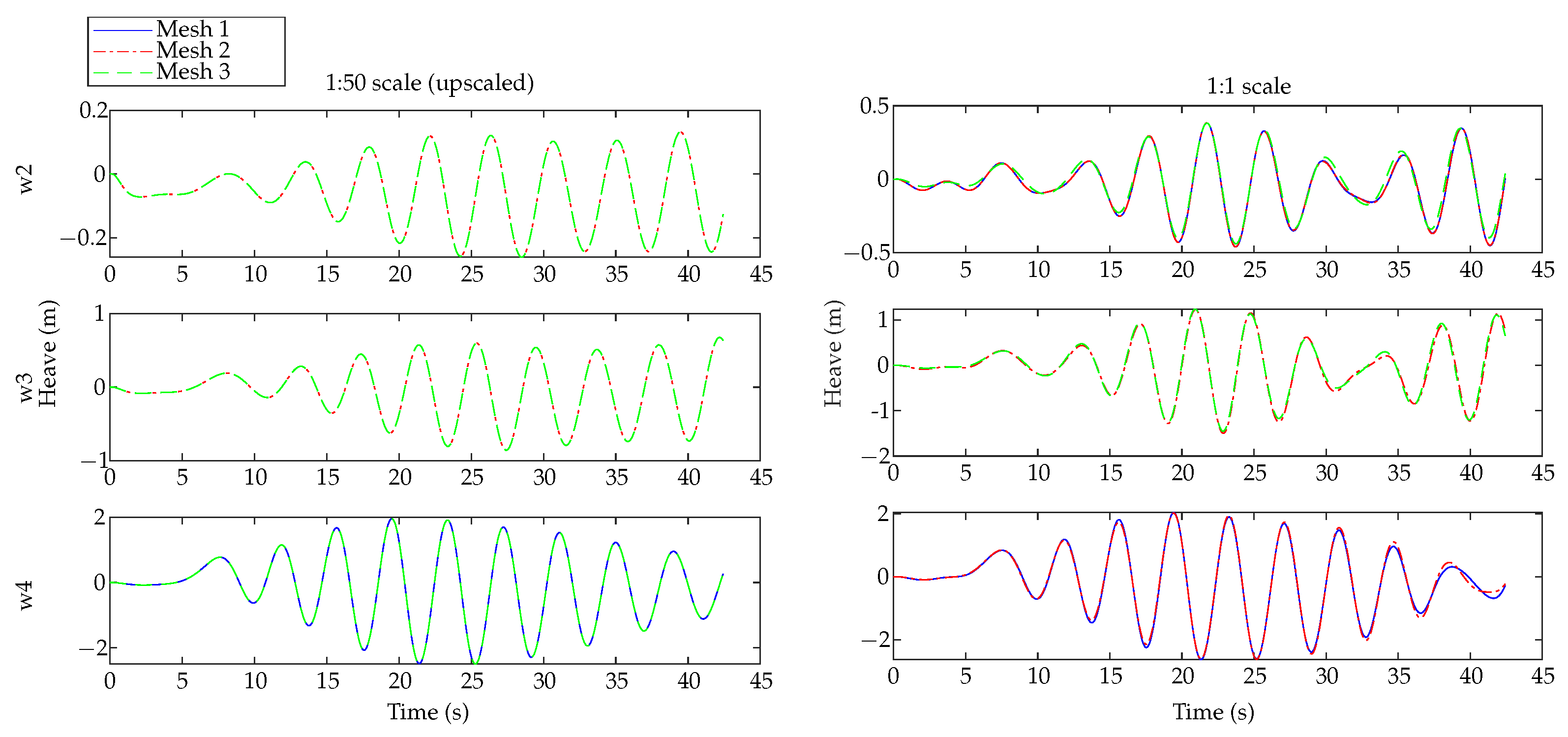
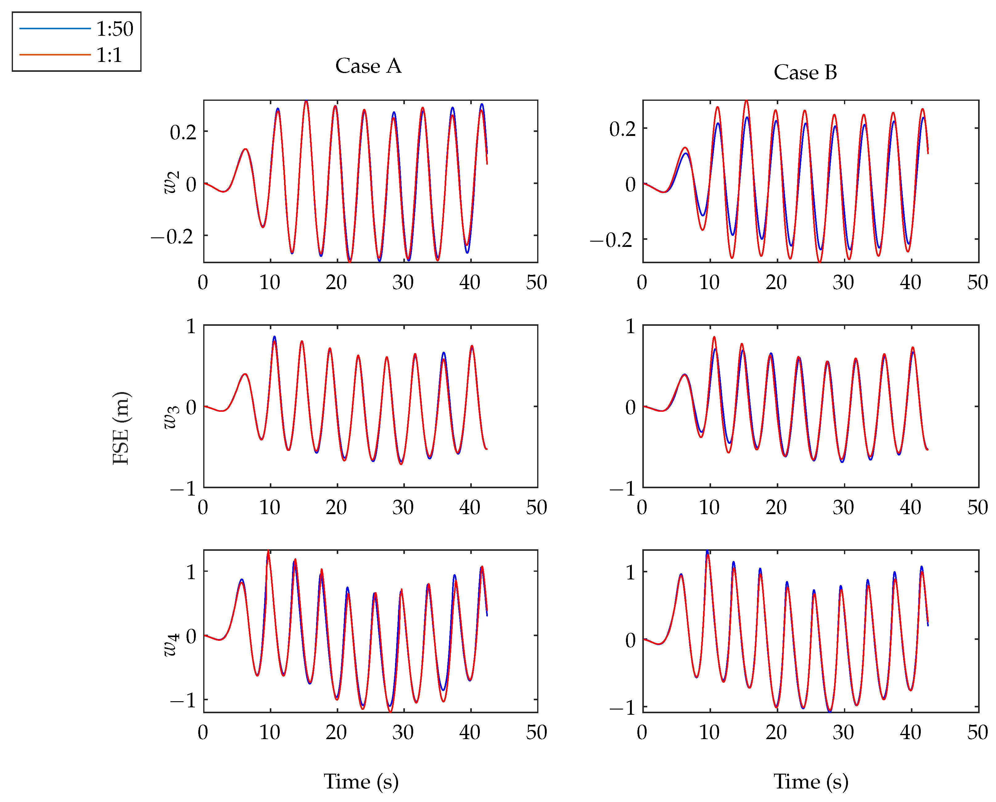
In first instance, the free surface elevation (FSE) is studied for the case without the buoy (Case A) at the middle of the width $W_t$ and at one wavelength from the inlet, for every studied case independently for scale 1:1 and scale 1:50. Results of the free surface elevation are illustrated in Figure 4, where the 1:50 scale is rescaled to be compared with the 1:1 cases. The same procedure is made for case B with the WEC present and results are shown in Figure 5. For case B, the heave motion of the WEC is also studied to ensure the correct mesh convergence, as shown in Figure 6.

Results in Figure 4, Figure 5 and Figure 6 show graphically that the differences between Mesh 2 and Mesh 3 and, in most cases, also Mesh 1, are negligible for all waves conditions in the two scales and with or without WEC. The normalised difference is calculated and shown in

Table 7. Difference $\epsilon$ between different mesh sizes, for all studied cases.

	Scale	Wave	Mesh 1/Mesh 2	Mesh 2/Mesh 3
Case A	1:1	$w_2$	0.470%	0.079%
		$w_3$	0.036%	0.109%
		$w_4$	0.107%	1.152%
	1:50	$w_2$	0.016%	0.202%
		$w_3$	0.014%	0.021%
		$w_4$	1.041%	0.434%
Case B	1:1	$w_2$	0.035%	0.452%
		$w_3$	0.213%	0.085%
		$w_4$	0.292%	0.021%
	1:50	$w_2$	2.073%	0.322%
		$w_3$	0.234%	0.846%
		$w_4$	0.875%	0.034%
Heave	1:1	$w_2$	0.012%	1.931%
		$w_3$	0.134%	0.705%
		$w_4$	0.383%	0.473%
	1:50	$w_2$	2.076%	0.854%
		$w_3$	0.348%	0.034%
		$w_4$	0.871%	0.084%

, where it can be seen that the difference from results obtained using different meshes are always below 3% and in most cases below 1%, which ensures that when using Mesh 2 or Mesh 3, the results will be mesh independent. The normalised difference $\epsilon$ is calculated according to the norm of the difference divided by the norm of the reference term.

4. Results and Discussion

In order to compare the results, two different analyses are made. First, the scale effect is studied and then the order effect is analysed. A rescale procedure is performed according to the scale factors defined by Froude similarity to compare the behaviour of the scale effect in the different models at the same time domain. The Froude scaling ratio are shown in

Table 8. Froude scaling ratio.

Parameter	Froude Scaling Ratio
Length	$\Lambda$
Time	${\Lambda }^{1/2}$
Mass	${\Lambda }^3$
Power	${\Lambda }^{7/2}$

, where $\Lambda$ is the geometric scale relation, in this case 1/50.

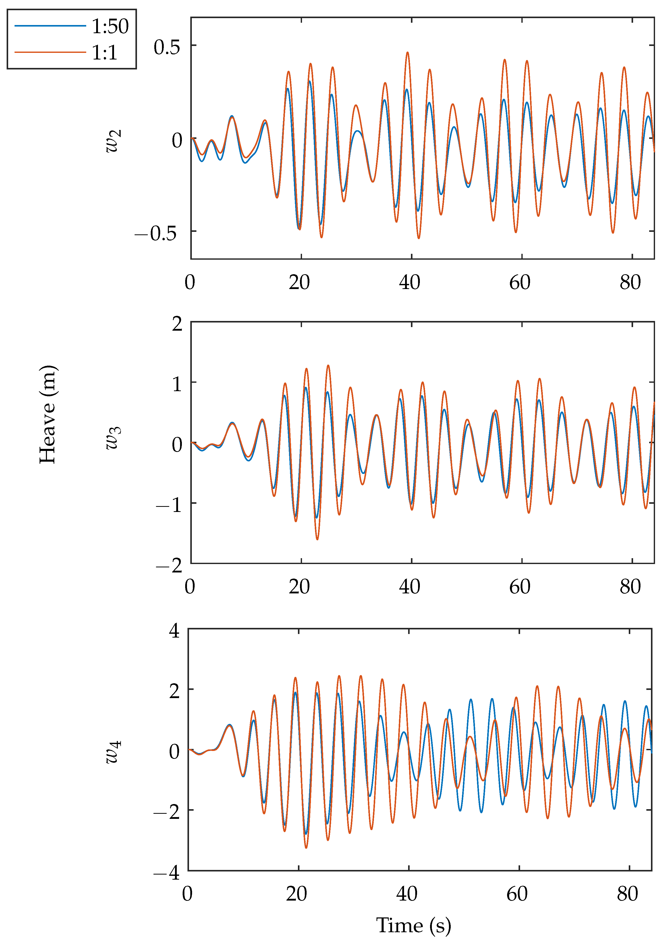
The free surface elevation at the middle of the width $W_t$ and at one wavelength from the inlet is compared between the two scales, and it is shown in Figure 7 for the cases without (Case A) and with WEC (Case B). The heave movement of the WEC is shown in Figure 8 for the 1:1 case and 1:50 case. The latter is upscaled so that all presented results in this section are natural scale. In these figures, the three waves conditions are presented for the recommended wave model.

Figure 8 shows the heave movement for scale 1:1 and scale 1:50 for the three waves conditions using the recommended wave theory. The differences from the FSE between the two scales of the cases shown in Figure 7 and from the heave motion shown in Figure 8 are summarised in

Table 9. Normalised difference $\epsilon$ between scales, for the three cases analysed using the recommended wave theory.

	${\mathit{w}}_2$	${\mathit{w}}_3$	${\mathit{w}}_4$
Case A FSE	1.09%	0.58%	3.05%
Case B FSE	6.46%	3.00%	0.59%
Case B Heave	38.0%	30.0%	56.0%

.

From these figures and table we can conclude that the scale effect on the free surface elevation is lower than 6.5% for all cases, which could be considered negligible in most cases. Nevertheless, differences for heave motion are between 30% and 56%, which could be important for most applications. Results shown in Figure 8 also show that for these three cases, the motion in 1:1 scale is higher than the case 1:50, which could be attributed to drag forces that reduce the movement in 1:50 scale compared with scale 1:1, where these forces are less predominant.

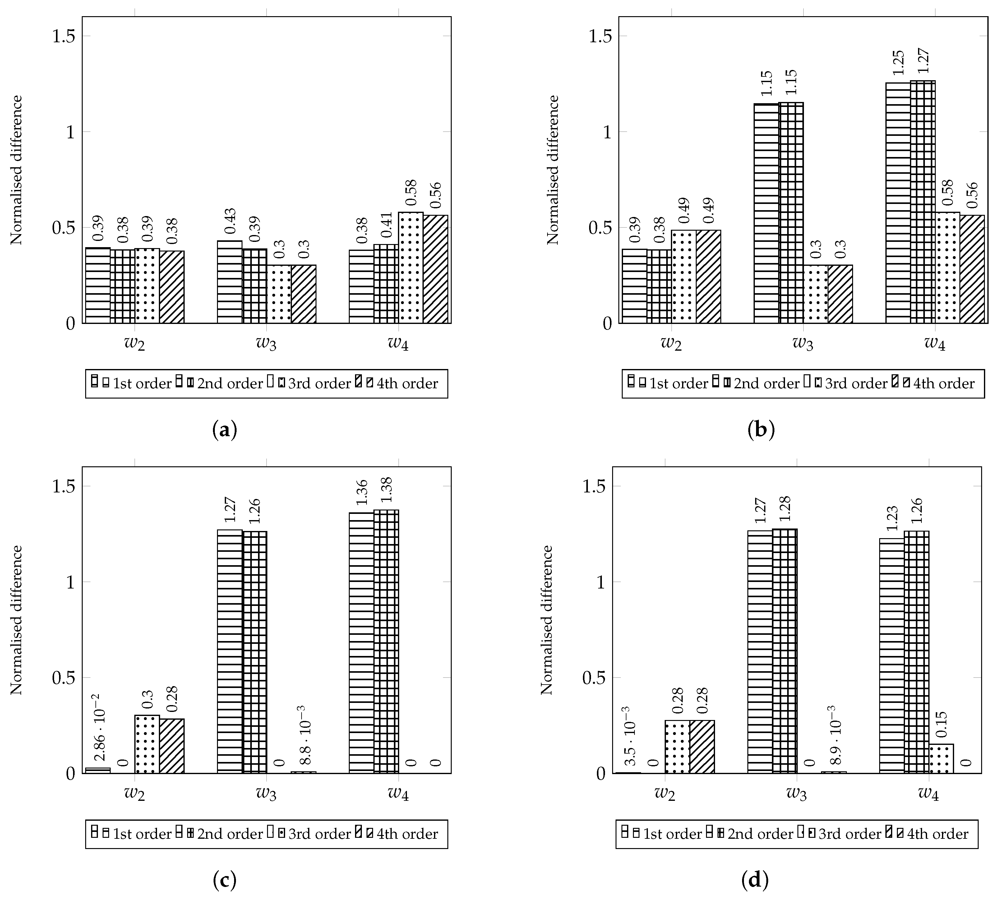
The second analysis is based on the study of the wave order theory behaviour for each studied case and how these theories affect the difference between scales. This analysis is made including only the first 80 seconds of the simulation. In order to achieve the described goal, the normalised difference $\epsilon$ between rescaled heave displacement of the WEC using scale 1:50 and heave for scale 1:1 is shown in Figure 9. In this figure, each difference is obtained using the same wave order theory. For example the first column indicates the differences of heave between scale 1:1 and upscaled 1:50, for a wave $w_2$ modelled using first order wave theory in both cases.

Results shown in Figure 9a indicate that for most waves the difference fluctuates between 30% and 43%. These differences can be originated due to the viscous and other nonlinear effects that become relevant. There are two waves that present higher differences of 58% and 56% for 3rd and 4th order theories respectively for wave $w_4$. This behaviour may be explained by a more significant change in the modulating frequency than in the other cases. This modulating frequency is due to the transient effect that disappears after some seconds. This may reduce the difference for these cases in the stationary regime.

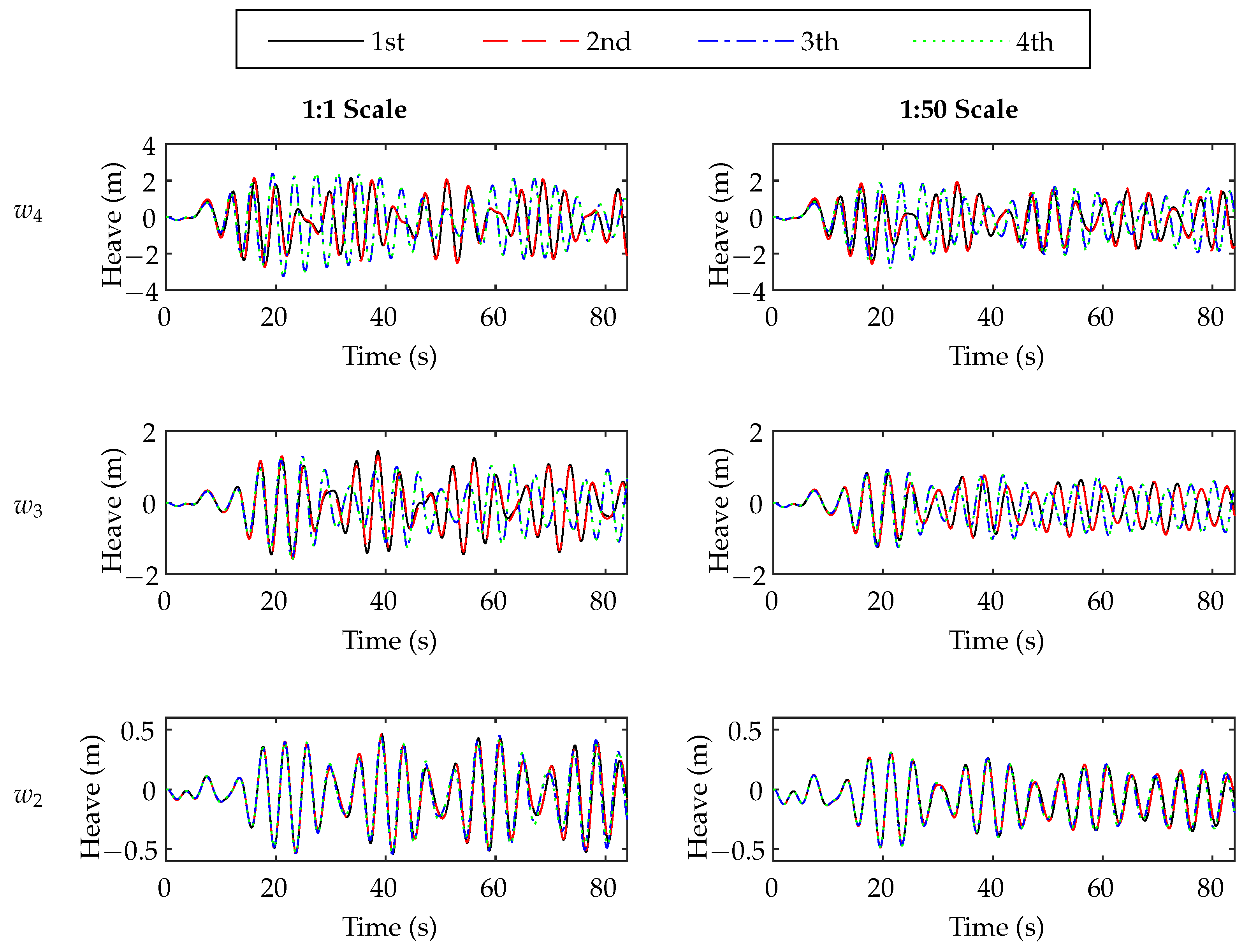
In Figure 9b the normalised difference $\epsilon$ between rescaled heave displacement of the WEC using scale 1:50 and the recommended order theory for scale 1:1 is shown. Figure 9c,d show the normalised difference $\epsilon$ between heave displacement of the WEC using the four different order models compared to the recommended order, for scale 1:1 and scale 1:50, respectively. It is important to mention that the wrong selection of wave theory can lead to differences up to 138%. In Figure 10 the variation of the heave movement in time is shown for the three waves ($w_2$, $w_3$ and $w_4$) and for the four order theories, for case 1:1 at the left hand side and 1:50 at the right hand side.

Figure 9 and Figure 10 show that in all cases the recommended order is the one that presents lower differences. Nevertheless, almost the same difference is found for the 1st and 2nd order in the three cases studied and also the same difference is found for the 3rd and 4th order for all cases.

Due to the fact that the difference between 1st or 2nd order in case $w_2$ are lower than 3%, it can be concluded that the range of applicability of linear theory could by higher than the recommended range for this problem. It is also possible to see that the difference between 3rd or 4th order theories for cases $w_3$ and $w_4$ is lower than 1% in scale 1:50 and lower than 15% for scale 1:1, showing a higher range of applicability for 3rd order theory at least for 1:50 scale.

5. Conclusions

Results show that the normalised difference of the WEC motion between the same order theory for scale 1:50 and 1:1 fluctuate between 30% and 58% for the WEC heave motion. This can indicate that the scale effects are relevant, and, depending on the accuracy of the expected results, viscous effects have to be taken into account in the scale procedure. Additionally, the higher differences are found in the waves with higher steepness $w_4$. In this case, a change in the modulation of the wave is found due to the transient effect, which increases the difference. This indicates that the wave steepness and in consequence the wave theory affects the difference for transient analysis. It is also possible to conclude that the wrong selection of the wave theory can lead to differences up to 138% for the WEC heave motion. Finally, it is important to mention that the range of applicability of the different order theories should be studied for each case. The results from this work show that the same difference is found for 1st and 2nd order in all cases and the same behaviour is found for 3rd and 4th order, which indicates that the use of linear theory can be extended for a higher range and the same is found for third order theory.

References

- Salter, S. Wave power. Nature 1974, 7720, 249–260. [Google Scholar] [CrossRef]
- Mørk, G.; Barstow, S.; Kabuth, A.; Pontes, M.T. Assessing the global wave energy potential. In Proceedings of the International Conference on Offshore Mechanics and Arctic Engineering—OMAE, Shanghai, China, 6–11 June 2010; Volume 3, pp. 447–454. [Google Scholar]
- Noble, D.R.; O’Shea, M.; Judge, F.; Robles, E.; Martinez, R.; Khalid, F.; Thies, P.R.; Johanning, L.; Corlay, Y.; Gabl, R.; et al. Standardising Marine Renewable Energy Testing: Gap Analysis and Recommendations for Development of Standards. J. Mar. Sci. Eng. 2021, 9, 971. [Google Scholar] [CrossRef]
- Ticona Rollano, F.; Tran, T.T.; Yu, Y.H.; García-Medina, G.; Yang, Z. Influence of Time and Frequency Domain Wave Forcing on the Power Estimation of a Wave Energy Converter Array. J. Mar. Sci. Eng. 2020, 8, 171. [Google Scholar] [CrossRef] [Green Version]
- Cabral, T.; Clemente, D.; Rosa-Santos, P.; Taveira-Pinto, F.; Morais, T.; Belga, F.; Cestaro, H. Performance Assessment of a Hybrid Wave Energy Converter Integrated into a Harbor Breakwater. Energies 2020, 13, 236. [Google Scholar] [CrossRef] [Green Version]
- Musiedlak, P.H.; Ransley, E.J.; Hann, M.; Child, B.; Greaves, D.M. Time-Splitting Coupling of WaveDyn with OpenFOAM by Fidelity Limit Identified from a WEC in Extreme Waves. Energies 2020, 13, 3431. [Google Scholar] [CrossRef]
- Quartier, N.; Ropero-Giralda, P.; Domínguez, J.M.; Stratigaki, V.; Troch, P. Influence of the Drag Force on the Average Absorbed Power of Heaving Wave Energy Converters Using Smoothed Particle Hydrodynamics. Water 2021, 13, 384. [Google Scholar] [CrossRef]
- Ropero-Giralda, P.; Crespo, A.J.C.; Coe, R.G.; Tagliafierro, B.; Domínguez, J.M.; Bacelli, G.; Gómez-Gesteira, M. Modelling a Heaving Point-Absorber with a Closed-Loop Control System Using the DualSPHysics Code. Energies 2021, 14, 760. [Google Scholar] [CrossRef]
- Verao Fernandez, G.; Stratigaki, V.; Quartier, N.; Troch, P. Influence of Power Take-Off Modelling on the Far-Field Effects of Wave Energy Converter Farms. Water 2021, 13, 429. [Google Scholar] [CrossRef]
- Balitsky, P.; Quartier, N.; Stratigaki, V.; Verao Fernandez, G.; Vasarmidis, P.; Troch, P. Analysing the Near-Field Effects and the Power Production of Near-Shore WEC Array Using a New Wave-to-Wire Model. Water 2019, 11, 1137. [Google Scholar] [CrossRef] [Green Version]
- Šljivac, D.; Temiz, I.; Nakomčić-Smaragdakis, B.; Žnidarec, M. Integration of Wave Power Farms into Power Systems of the Adriatic Islands: Technical Possibilities and Cross-Cutting Aspects. Water 2021, 13, 13. [Google Scholar] [CrossRef]
- Sheng, W.; Alcorn, R.; Lewis, T. Physical modelling of wave energy converters. Ocean. Eng. 2014, 84, 29–36. [Google Scholar] [CrossRef]
- IEC TS 62600; Wave, Tidal and Other Water Current Converters—Part 103: Guidelines for the Early Stage Development of Wave Energy Converters—Best Practices and Recommended Procedures for the Testing of Pre-Prototype Devices. International Electrotechnical Commission: Geneva, Switzerland, 2018.
- Davey, T.; Sarmiento, J.; Ohana, J.; Thiebaut, F.; Haquin, S.; Weber, M.; Gueydon, S.; Judge, F.; Lyden, E.; O’Shea, M.; et al. Round Robin Testing: Exploring Experimental Uncertainties through a Multifacility Comparison of a Hinged Raft Wave Energy Converter. J. Mar. Sci. Eng. 2021, 9, 946. [Google Scholar] [CrossRef]
- Assessment of Experimental Uncertainty for a Floating Wind Semisubmersible Under Hydrodynamic Loading. Volume 10: Ocean Renewable Energy. In Proceedings of the International Conference on Offshore Mechanics and Arctic Engineering, Madrid, Spain, 17–22 June 2018. [CrossRef]
- BMT Fluid Mechanics Ltd. Review of Model Testing Requirements for FPSO’s; BMT Fluid Mechanics Ltd.: Teddington, UK, 2001; pp. 1–80. [Google Scholar]
- Heller, V. Scale effects in physical hydraulic engineering models. J. Hydraul. Res. 2011, 49, 293–306. [Google Scholar] [CrossRef]
- Schmitt, P.; Elsäßer, B. The application of Froude scaling to model tests of Oscillating Wave Surge Converters. Ocean. Eng. 2017, 141, 108–115. [Google Scholar] [CrossRef] [Green Version]
- Palm, J.; Eskilsson, C.; Bergdahl, L.; Bensow, R.E. Assessment of scale effects, viscous forces and induced drag on a point-absorbing wave energy converter by CFD simulations. J. Mar. Sci. Eng. 2018, 6, 124. [Google Scholar] [CrossRef] [Green Version]
- Windt, C.; Ringwood, J.V.; Davidson, J.; Schmitt, P. Contribution to the ccp-wsi blind test series 3: Analysis of scaling effects of moored point-absorber wave energy converters in a cfd-based numerical wave tank. In Proceedings of the International Offshore and Polar Engineering Conference, Honolulu, HI, USA, 16–21 June 2019; Volume 3, pp. 3051–3058. [Google Scholar]
- Windt, C.; Davidson, J.; Ringwood, J.V. Numerical analysis of the hydrodynamic scaling effects for the Wavestar wave energy converter. J. Fluids Struct. 2021, 105, 103328. [Google Scholar] [CrossRef]
- Le Méhauté, B. An Introduction to Hydrodynamics and Water Waves; Springer: New York, NY, USA, 1976. [Google Scholar]
- Hedges, T.; URSELL. Regions of validity of analytical wave theories. Proc. Inst. Civ. Eng.-Water Marit. Energy 1995, 112, 111–114. [Google Scholar] [CrossRef]
- Finnegan, W.; Rosa-Santos, P.; Taveira-Pinto, F.; Goggins, J. Development of a numerical model of the CECO wave energy converter using computational fluid dynamics. Ocean. Eng. 2021, 219, 108416. [Google Scholar] [CrossRef]
- Schubert, B.W.; Robertson, W.S.; Cazzolato, B.S.; Ghayesh, M.H. Linear and nonlinear hydrodynamic models for dynamics of a submerged point absorber wave energy converter. Ocean. Eng. 2020, 197, 106828. [Google Scholar] [CrossRef]
- Sjökvist, L.; Wu, J.; Ransley, E.; Engström, J.; Eriksson, M.; Göteman, M. Numerical models for the motion and forces of point-absorbing wave energy converters in extreme waves. Ocean. Eng. 2017, 145, 1–14. [Google Scholar] [CrossRef] [Green Version]
- Al Shami, E.; Wang, Z.; Wang, X. Non-linear dynamic simulations of two-body wave energy converters via identification of viscous drag coefficients of different shapes of the submerged body based on numerical wave tank CFD simulation. Renew. Energy 2021, 179, 983–997. [Google Scholar] [CrossRef]
- Bharath, A.; Nader, J.R.; Penesis, I.; Macfarlane, G. Nonlinear hydrodynamic effects on a generic spherical wave energy converter. Renew. Energy 2018, 118, 56–70. [Google Scholar] [CrossRef]
- Benites-Munoz, D.; Huang, L.; Anderlini, E.; Marín-Lopez, J.R.; Thomas, G. Hydrodynamic modelling of an oscillating wave surge converter including power take-off. J. Mar. Sci. Eng. 2020, 8, 771. [Google Scholar] [CrossRef]
- Airy, G. Tides and Waves. Encycl. Metrop. 1845, 5, 341–396. [Google Scholar]
- Fluent, A. ANSYS Fluent Theory Guide 2019R3; ANSYS: Canonsburg, PA, USA, 2019; pp. 561–734. [Google Scholar]
- Stokes, G. On the theory of oscillatory waves. Trans. Camb. Philos. Soc. 1847, 8, 441–455. [Google Scholar]
- Fenton, J.D. Nonlinear wave theories. Sea 1990, 9, 3–25. [Google Scholar]
- Penalba, M.; Giorgi, G.; Ringwood, J.V. Mathematical modelling of wave energy converters: A review of nonlinear approaches. Renew. Sustain. Energy Rev. 2017, 78, 1188–1207. [Google Scholar] [CrossRef] [Green Version]
- Li, Y.; Yu, Y.H. A synthesis of numerical methods for modeling wave energy converter-point absorbers. Renew. Sustain. Energy Rev. 2012, 16, 4352–4364. [Google Scholar] [CrossRef]
- Martínez-Ferrer, P.J.; Qian, L.; Ma, Z.; Causon, D.M.; Mingham, C.G. Improved numerical wave generation for modelling ocean and coastal engineering problems. Ocean. Eng. 2018, 152, 257–272. [Google Scholar] [CrossRef] [Green Version]
- Bharath, A.; Penesis, I.; Nader, J.r.; Macfarlane, G. Non-Linear CFD Modelling of a Submerged Sphere Wave Energy Converter. In Proceedings of the 3rd Asian Wave and Tidal Energy Conference, Singapore, 24–28 October 2016; pp. 1–10. [Google Scholar]
- Bouali, B.; Larbi, S. Contribution to the geometry optimization of an oscillating water column wave energy converter. Energy Procedia 2013, 36, 565–573. [Google Scholar] [CrossRef] [Green Version]
- Martin, D.; Parker, R.G.; Tafti, D.K. Hydrodynamic Design Optimization and Wave Tank Testing of a Self-Reacting Two-Body Wave Energy Converter. Ph.D. Thesis, Virginia Polytechnic Institute and State University, Blacksburg, VA, USA, 2017. [Google Scholar]
- Khedkar, K.; Nangia, N.; Thirumalaisamy, R.; Bhalla, A.P.S. The inertial sea wave energy converter (ISWEC) technology: Device-physics, multiphase modeling and simulations. Ocean. Eng. 2021, 229, 108879. [Google Scholar] [CrossRef]
- Yu, Y.H.; Li, Y. Reynolds-Averaged Navier-Stokes simulation of the heave performance of a two-body floating-point absorber wave energy system. Comput. Fluids 2013, 73, 104–114. [Google Scholar] [CrossRef]
- Devolder, B.; Stratigaki, V.; Troch, P.; Rauwoens, P. CFD simulations of floating point absorber wave energy converter arrays subjected to regular waves. Energies 2018, 11, 641. [Google Scholar] [CrossRef] [Green Version]
- Bhinder, M.A.; Babarit, A.; Gentaz, L.; Ferrant, P. Assessment of Viscous Damping via 3D-CFD Modelling of a Floating Wave Energy Device. In Proceedings of the European Wave and Tidal Energy Conference, EWTEC, Southampton, UK, 5–9 September 2011; pp. 1–6. [Google Scholar]
Figure 1.
Numerical wave tank and point absorber representation.
Figure 2.
Point absorber at laboratory scale.
Figure 3.
Mesh refinement zones.
Figure 4.
Mesh convergence analysis using free surface elevation at the middle of the width and at one wavelength from the inlet, for Case A.
Figure 5.
Mesh convergence analysis using free surface elevation at the middle of the width and at one wavelength from the inlet, for Case B.
Figure 6.
Mesh convergence analysis using heave motion for Case B.
Figure 7.
Free surface elevation at the middle of the width and at one wavelength from the inlet for cases , , and , using recommended order wave theory, for scales 1:1 and upscaled 1:50, using the wave tank without WEC at the left hand side and with WEC at the right hand side.
Figure 8.
Heave displacement for cases , , and , using recommended order wave theory, for scales 1:1 and upscaled 1:50.
Figure 9.
Normalised difference between heave displacement of the WEC. (a) Normalised difference between the same order model of scale 1:50 and scale 1:1. (b) Normalised difference between each model in scale 1:50 and recommended scale 1:1. (c) Normalised difference between different order models for scale 1:1. (d) Normalised difference between different order models for scale 1:50.
Figure 10.
Heave displacement for cases , and using 1st order, 2nd order, 3rd order and 4th order wave theories, for scales 1:1 and 1:50.