
Delineation of Groundwater Potential Zones (GWPZs) in a Semi-Arid Basin through Remote Sensing, GIS, and AHP Approaches

 ,
,  ,
,
Abstract
:1. Introduction
2. Materials and Methods
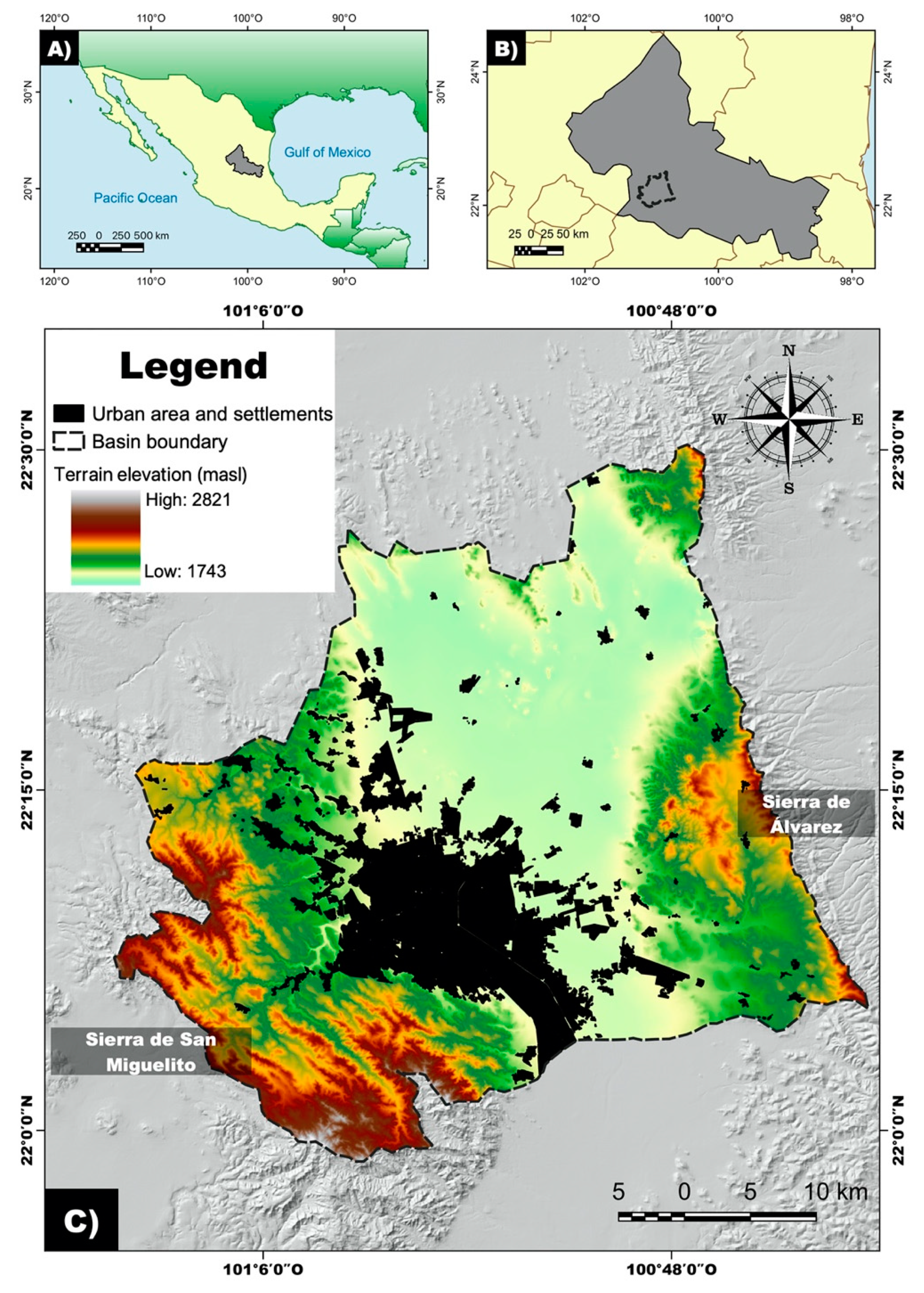
2.1. Study Area
2.1.1. Hydrographic Framework
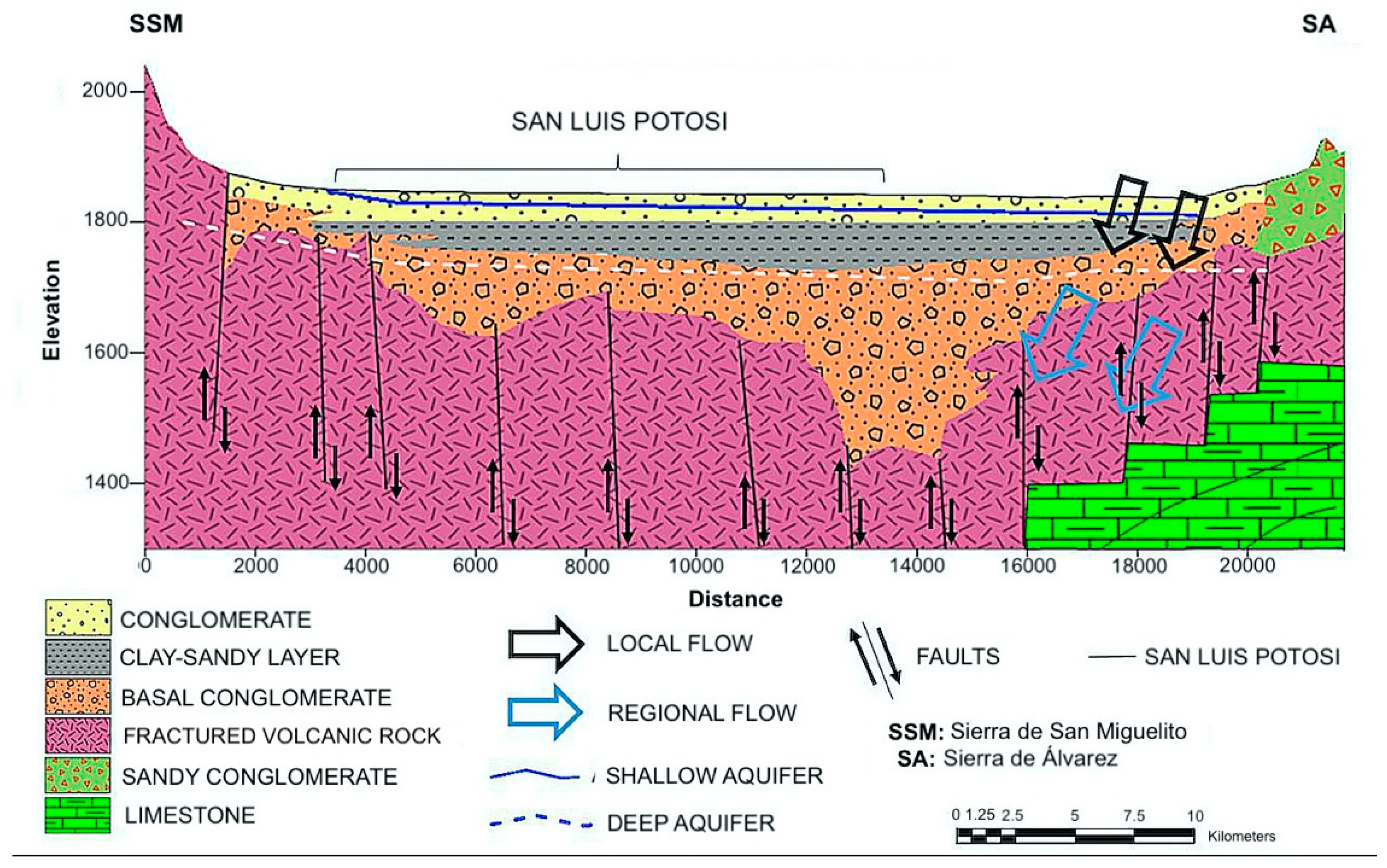
2.1.2. Geological and Hydrogeological Framework
2.1.3. Groundwater Extraction and Water Supply
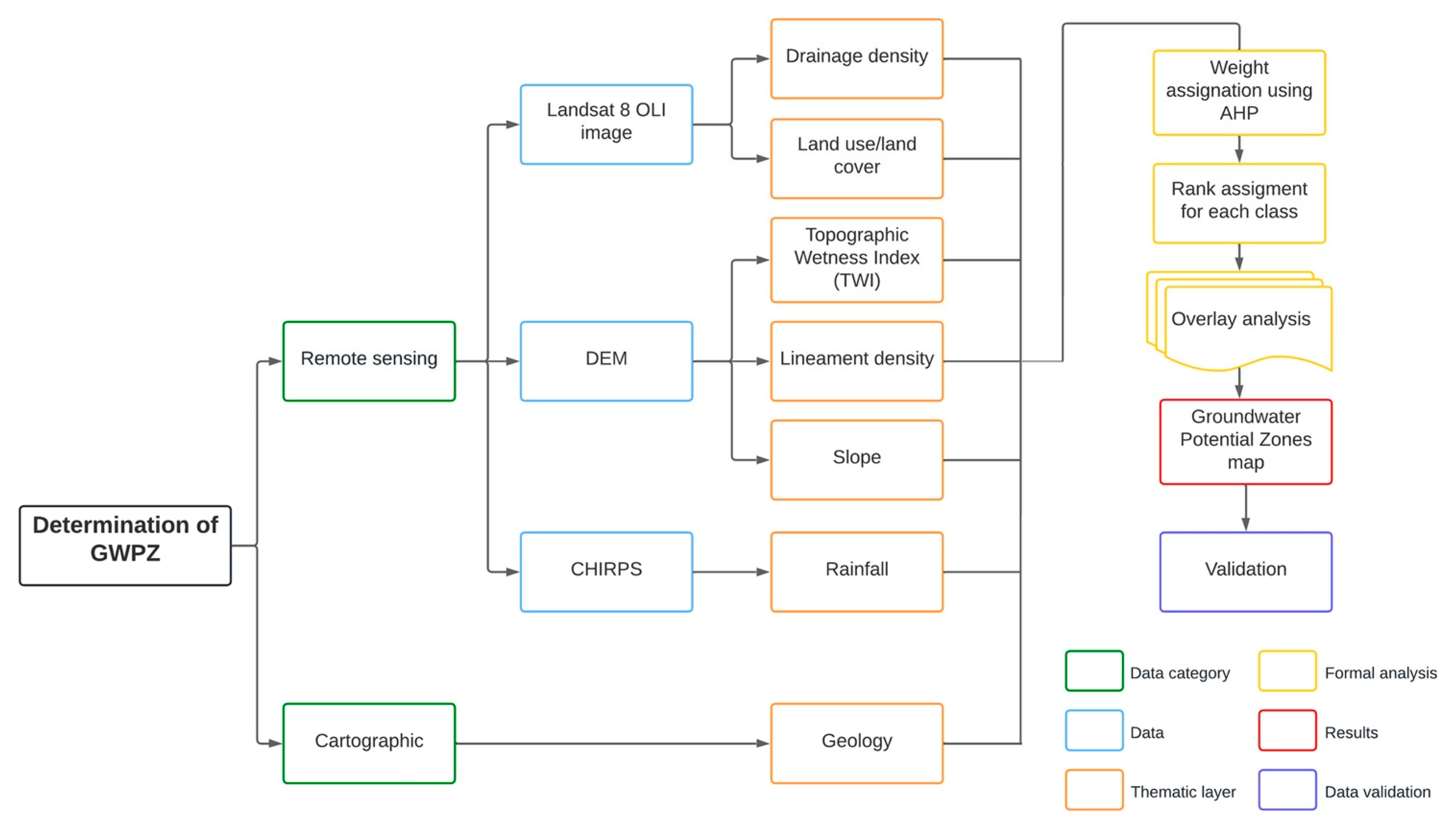
2.2. Methodology
2.2.1. Geology
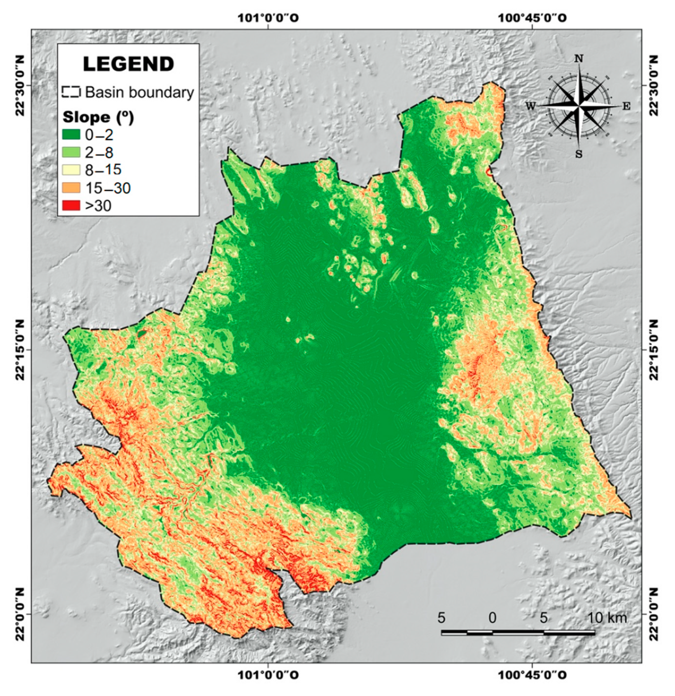
2.2.2. Slope
2.2.3. Lineament Density
2.2.4. Drainage Density (D)
2.2.5. Rainfall
2.2.6. Land Use and Land Cover (LULC)
2.2.7. Topographic Wetness Index (TWI)
2.2.8. Weight Calculation Using AHP
2.2.9. Mapping Groundwater Potential Zones (GWPZs)
2.2.10. Validation of Results
3. Results and Discussion
3.1. Description of Thematic Layers
3.1.1. Geology
3.1.2. Slope
3.1.3. Lineament Density
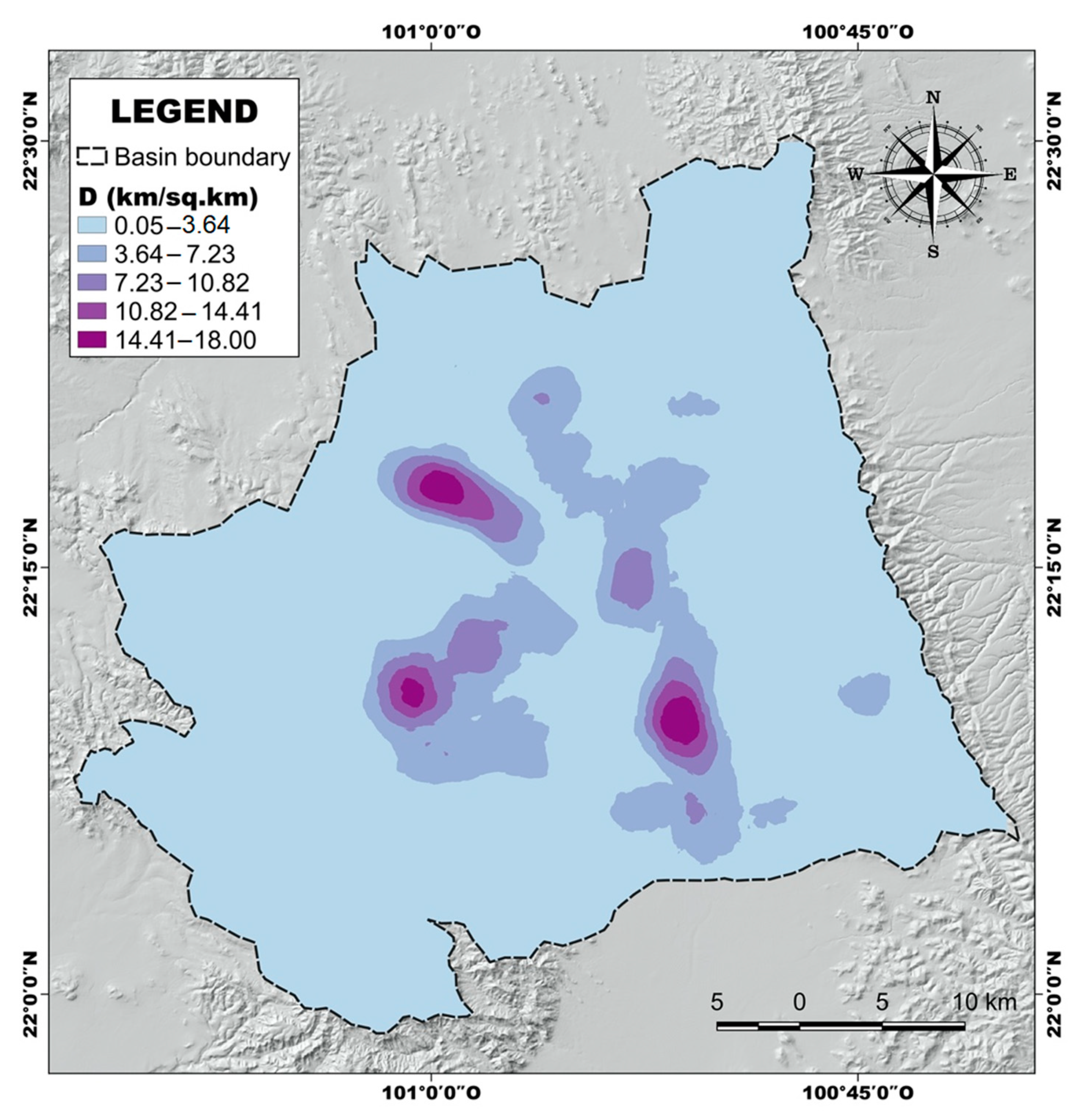
3.1.4. Drainage Density (D)
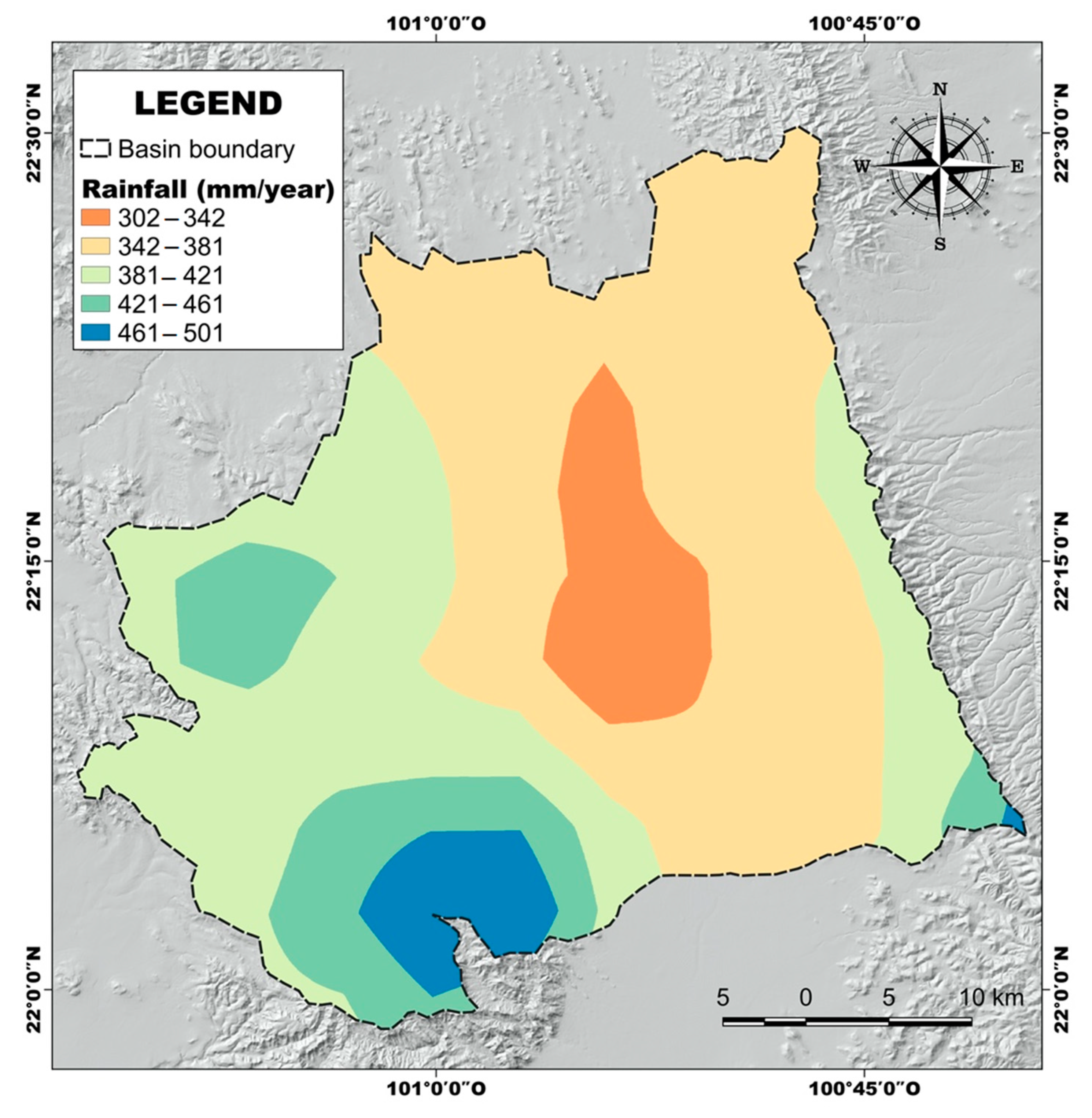
3.1.5. Rainfall
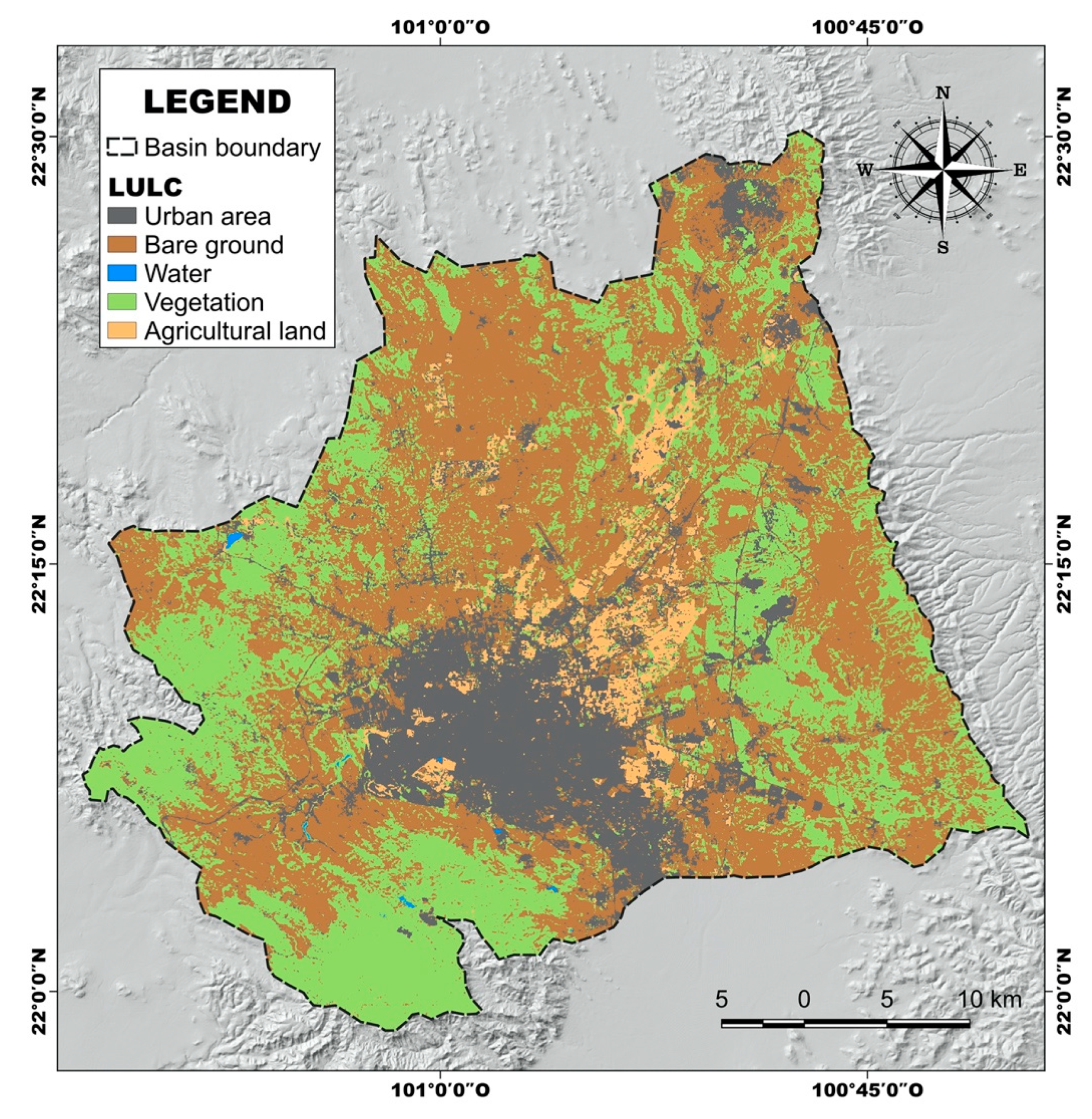
3.1.6. Land Use and Land Cover (LULC)
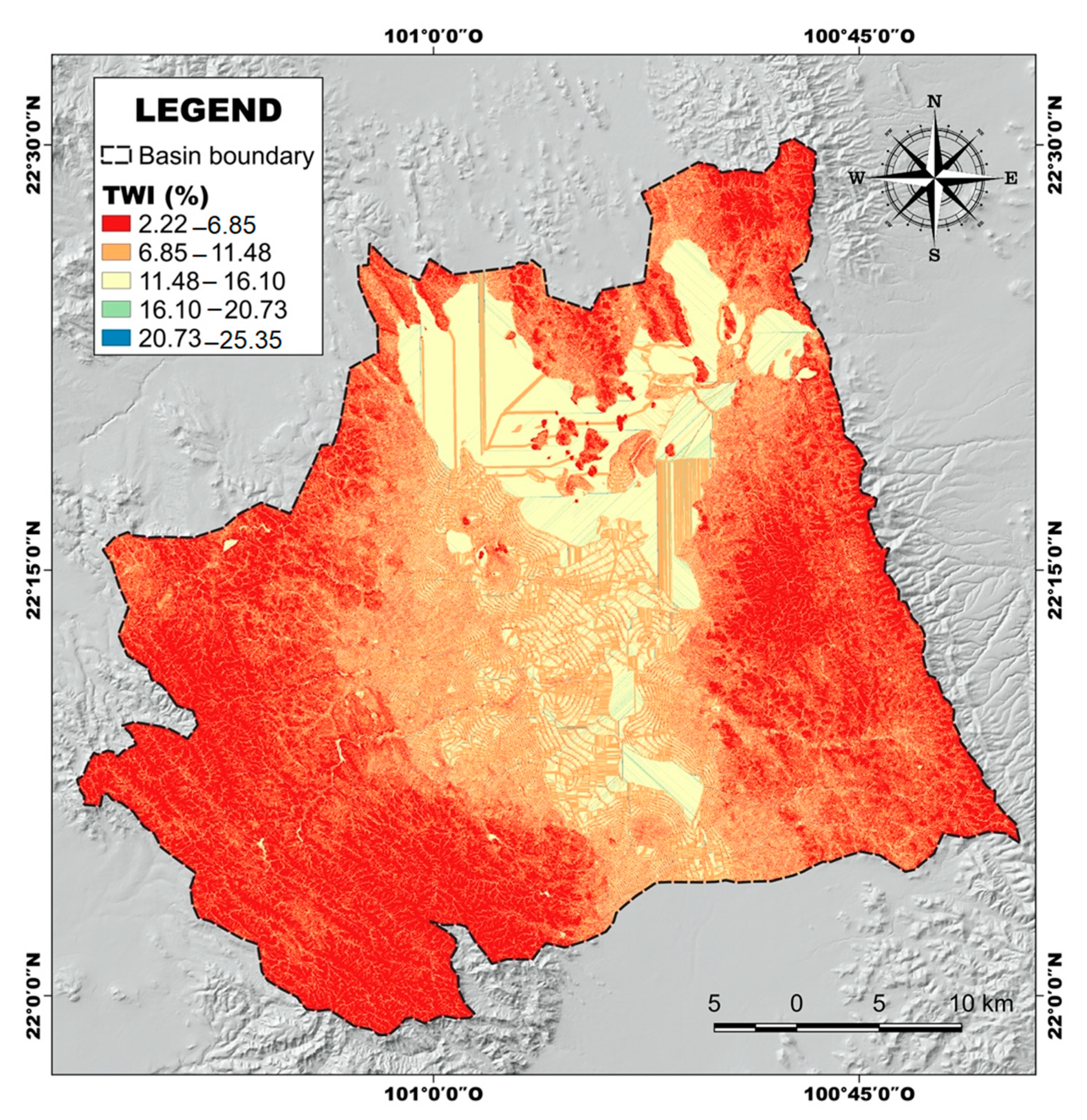
3.1.7. Topographic Wetness Index (TWI)
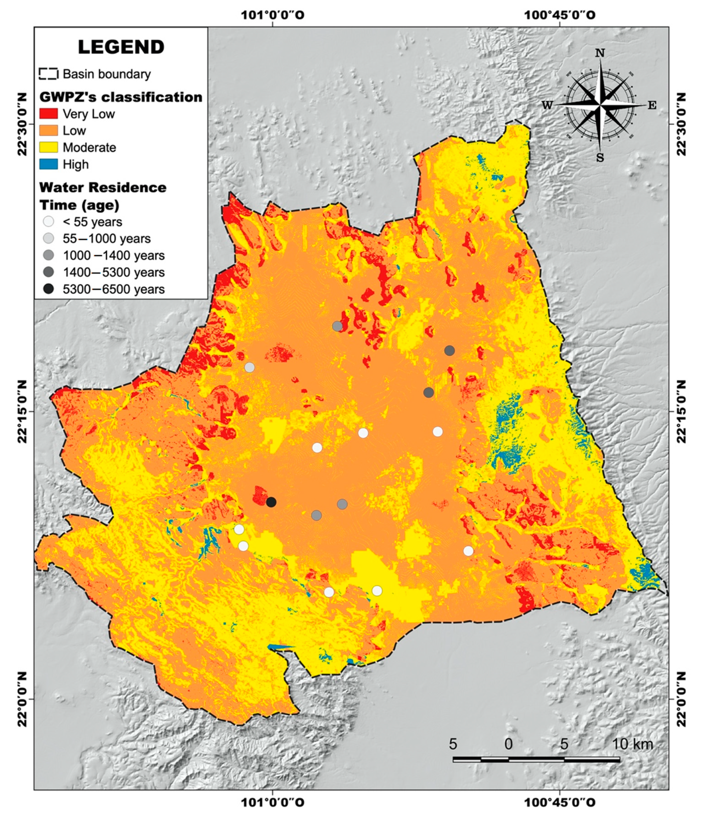
3.2. Mapping Groundwater Potential Zones (GWPZs)
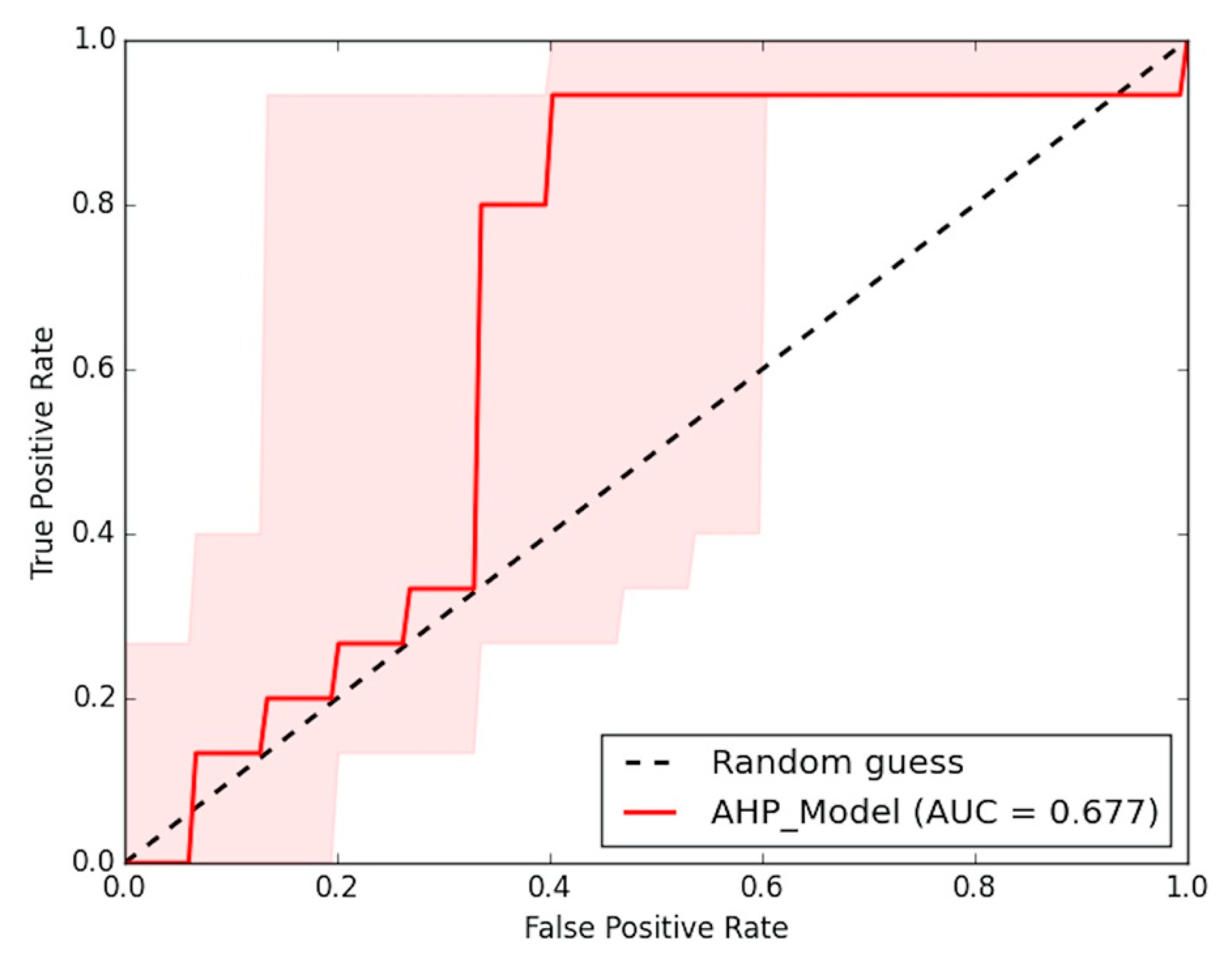
Validation of Results
3.3. Limitations of the Study
4. Conclusions
Supplementary Materials
Author Contributions
Funding
Institutional Review Board Statement
Informed Consent Statement
Data Availability Statement
Acknowledgments
Conflicts of Interest
References
- Makonyo, M.; Msabi, M.M. Identification of groundwater potential recharge zones using GIS-based multi-criteria decision analysis: A case study of semi-arid midlands Manyara fractured aquifer, North-Eastern Tanzania. Remote Sens. Appl. Soc. Environ. 2021, 23, 100544. [Google Scholar] [CrossRef]
- Ifediegwu, S.I. Assessment of groundwater potential zones using GIS and AHP techniques: A case study of the Lafia district, Nasarawa State, Nigeria. Appl. Water Sci. 2022, 12, 10. [Google Scholar] [CrossRef]
- Ghosh, A.; Adhikary, P.P.; Bera, B.; Bhunia, G.S.; Shit, P.K. Assessment of groundwater potential zone using MCDA and AHP techniques: Case study from a tropical river basin of India. Appl. Water Sci. 2022, 12, 37. [Google Scholar] [CrossRef]
- Chatterjee, S.; Dutta, S. Assessment of groundwater potential zone for sustainable water resource management in south-western part of Birbhum District, West Bengal. Appl. Water Sci. 2022, 12, 40. [Google Scholar] [CrossRef]
- Arulbalaji, P.; Padmalal, D.; Sreelash, K. GIS and AHP Techniques Based Delineation of Groundwater Potential Zones: A case study from Southern Western Ghats, India. Sci. Rep. 2019, 9, 2082. [Google Scholar] [CrossRef]
- Masoud, A.M.; Pham, Q.B.; Alezabawy, A.K.; Abu El-Magd, S.A. Efficiency of Geospatial Technology and Multi-Criteria Decision Analysis for Groundwater Potential Mapping in a Semi-Arid Region. Water 2022, 14, 882. [Google Scholar] [CrossRef]
- Suliman, M.; Samiullah, K.; Ali, M. Identification of potential groundwater recharge sitein a semi-arid region of pakistan using saaty’s analytical hierarchical process (Ahp). Geomat. Environ. Eng. 2022, 16, 53–70. [Google Scholar] [CrossRef]
- Sahu, U.; Wagh, V.; Mukate, S.; Kadam, A.; Patil, S. Applications of geospatial analysis and analytical hierarchy process to identify the groundwater recharge potential zones and suitable recharge structures in the Ajani-Jhiri watershed of north Maharashtra, India. Groundw. Sustain. Dev. 2022, 17, 100733. [Google Scholar] [CrossRef]
- Dakhlalla, A.O.; Parajuli, P.B.; Ouyang, Y.; Schmitz, D.W. Evaluating the impacts of crop rotations on groundwater storage and recharge in an agricultural watershed. Agric. Water Manag. 2016, 163, 332–343. [Google Scholar] [CrossRef] [Green Version]
- Scanlon, B.R.; Keese, K.E.; Flint, A.L.; Flint, L.E.; Gaye, C.B.; Edmunds, W.M.; Simmers, I. Global synthesis of groundwater recharge in semi-arid andaridregions. Hydrol. Process. 2006, 20, 3335–3370. [Google Scholar] [CrossRef]
- Kumar, M.; Singh, S.K.; Kundu, A.; Tyagi, K.; Menon, J.; Frederick, A.; Raj, A.; Lal, D. GIS-based multi-criteria approach to delineate groundwater prospect zone and its sensitivity analysis. Appl. Water Sci. 2022, 12, 71. [Google Scholar] [CrossRef]
- Asgher, M.S.; Kumar, N.; Kumari, M.; Ahmad, M.; Sharma, L.; Naikoo, M.W. Groundwater potential mapping of Tawi River basin of Jammu District, India, using geospatial techniques. Environ. Monit. Assess. 2022, 194, 240. [Google Scholar] [CrossRef] [PubMed]
- Dar, I.A.; Sankar, K.; Dar, M.A. Deciphering groundwater potential zones in hard rock terrain using geospatial technology. Environ. Monit. Assess. 2010, 173, 597–610. [Google Scholar] [CrossRef] [PubMed]
- Thapa, R.; Gupta, S.; Guin, S.; Kaur, H. Assessment of groundwater potential zones using multi-influencing factor (MIF) and GIS: A case study from Birbhum district, West Bengal. Appl. Water Sci. 2017, 7, 4117–4131. [Google Scholar] [CrossRef]
- Lentswe, G.B.; Molwalefhe, L. Delineation of potential groundwater recharge zones using analytic hierarchy process-guided GIS in the semi-arid Motloutse watershed, eastern Botswana. J. Hydrol. Reg. Stud. 2020, 28, 100674. [Google Scholar] [CrossRef]
- Malczewski, J.; Rinner, C. Multicriteria Decision Analysis in Geographic Information Science, 1st ed.; Springer: New York, NY, USA, 2015; ISBN 978-3-540-74757-4. [Google Scholar]
- Noyola-Medrano, M.C.; Ramos-Leal, J.A.; Domínguez-Mariani, E.; Pineda-Martínez, L.F.; López-Loera, H.; Carbajal, N. Factores que dan origen al minado de acuíferos en ambientes áridos: Caso Valle de San Luis Potosí. Rev. Mex. Cienc. Geol. 2009, 26, 395–410. [Google Scholar]
- Flores-Márquez, E.L.; Ledesma, I.K.; Arango-Galván, C. Sustainable geohydrological model of San Luis Potosí aquifer, Mexico. Geofísica Int. 2011, 50, 425–438. [Google Scholar] [CrossRef]
- López-Álvarez, B.; Ramos-Leal, J.A.; Carbajal, N.; Hernández-García, G.; Morán-Ramírez, J.; Santacruz-DeLeón, G. Modeling of Groundwater Flow and Water Use for San Luis Potosí Valley Aquifer System. J. Geogr. Geol. 2014, 6, 147–161. [Google Scholar] [CrossRef]
- López-Loera, H.; Ramos-Leal, J.A.; Dávila-Harris, P.; Torres-Gaytan, D.E.; Martinez-Ruiz, V.J.; Gogichaishvili, A. Geophysical Exploration of Fractured-Media Aquifers at the Mexican Mesa Central: Satellite City, San Luis Potosí, Mexico. Surv. Geophys. 2014, 36, 167–184. [Google Scholar] [CrossRef]
- Al-Djazouli, M.O.; Elmorabiti, K.; Rahimi, A.; Amellah, O.; Fadil, O.A.M. Delineating of groundwater potential zones based on remote sensing, GIS and analytical hierarchical process: A case of Waddai, eastern Chad. GeoJournal 2021, 86, 1881–1894. [Google Scholar] [CrossRef]
- Abdelouhed, F.; Ahmed, A.; Abdellah, A.; Yassine, B.; Mohammed, I. Using GIS and remote sensing for the mapping of potential groundwater zones in fractured environments in the CHAOUIA-Morocco area. Remote Sens. Appl. Soc. Environ. 2021, 23, 100571. [Google Scholar] [CrossRef]
- Muthu, K.; Sudalaimuthu, K. Integration of Remote sensing, GIS, and AHP in demarcating groundwater potential zones in Pattukottai Taluk, Tamilnadu, India. Arab. J. Geosci. 2021, 14, 1748. [Google Scholar] [CrossRef]
- Khan, M.Y.A.; ElKashouty, M.; Tian, F. Mapping Groundwater Potential Zones Using Analytical Hierarchical Process and Multicriteria Evaluation in the Central Eastern Desert, Egypt. Water 2022, 14, 1041. [Google Scholar] [CrossRef]
- Saaty, T.L. The Analytic Hierarchy Process: Planning, Priority Setting, Resources Allocation; McGraw: New York, NY, USA, 1980; ISBN 978-0070543713. [Google Scholar]
- Sajil-Kumar, P.J.; Elango, L.; Schneider, M. GIS and AHP Based Groundwater Potential Zones Delineation in Chennai River Basin (CRB), India. Sustainability 2022, 14, 1830. [Google Scholar] [CrossRef]
- Dhar, A.; Sahoo, S.; Sahoo, M. Identification of groundwater potential zones considering water quality aspect. Environ. Earth Sci. 2015, 74, 5663–5675. [Google Scholar] [CrossRef]
- Esquivel, J.M.; Morales, G.P.; Esteller, M.V. Groundwater Monitoring Network Design Using GIS and Multicriteria Analysis. Water Resour. Manag. 2015, 29, 3175–3194. [Google Scholar] [CrossRef]
- Flores, H.; Morales, J.L.; Mora-Rodríguez, J.; Carreño, G.; Delgado-Galván, X. Management priorities for aquifers in El Bajío in Guanajuato state, Mexico. Water Policy 2018, 20, 1161–1175. [Google Scholar] [CrossRef]
- Hernández-Marín, M.; Guerrero-Martínez, L.; Zermeño-Villalobos, A.; Rodríguez-González, L.; Burbey, T.J.; Pacheco-Martínez, J.; Martínez-Martínez, S.I.; González-Cervantes, N. Spatial and temporal variation of natural recharge in the semi-arid valley of Aguascalientes, Mexico. Hydrogeol. J. 2018, 26, 2811–2826. [Google Scholar] [CrossRef]
- Mendoza-Gómez, M.; Tagle-Zamora, D.; Morales Martínez, J.L.; Caldera Ortega, A.R.; Mora Rodríguez, J.D.J.; Delgado-Galván, X. Water Supply Management Index: Leon, Guanajuato, Mexico. Water 2022, 14, 919. [Google Scholar] [CrossRef]
- Ojeda-Olivares, E.A.; Belmonte-Jiménez, S.I.; Sandoval-Torres, S.; Campos-Enríquez, J.O.; Tiefenbacher, J.P.; Takaro, T.K. A simple method to evaluate groundwater vulnerability in urbanizing agricultural regions. J. Environ. Manag. 2020, 261, 110164. [Google Scholar] [CrossRef]
- Castro-Ovalle, A.G.; Tristán, A.C.; Amador-Nieto, J.A.; Putri, R.F.; Zahra, R.A. Analysing the land use/land cover influence on land surface temperature in San Luis Potosí Basin, México using remote sensing techniques. IOP Conf. Ser. Earth Environ. Sci. 2021, 686, 012029. [Google Scholar] [CrossRef]
- Interapas. Informe Anual 2020; Interapas: San Luis Potosí, Mexico, 2020. [Google Scholar]
- Cardona-Benavides, A.; Martínez-Hernández, J.E.; Alcalde-Alderete, R.; Larragoitia, J.C. La edad del agua subterránea que abastece la región de San Luis Potosí. Rev. Univ. Potos. 2006, 2, 20–25. [Google Scholar]
- Carrillo-Rivera, J.J. Hydrogeology of the San Luis Potosí Area, Mexico. Ph.D. Thesis, University of London, London, UK, 1992. [Google Scholar]
- Carrillo-Rivera, J.J. Application of the groundwater-balance equation to indicate interbasin and vertical flow in two semi-arid drainage basins, Mexico. Hydrogeol. J. 2000, 8, 503–520. [Google Scholar] [CrossRef]
- López-Álvarez, B.; Ramos-Leal, J.A.; Moran-Ramírez, J.; Cardona-Benavides, A.; Hernández-Garcia, G. Origen de la calidad del agua del acuífero colgado y su relación con los cambios de uso de suelo en el Valle de San Luis Potosí. Boletín De La Soc. Geológica Mex. 2013, 65, 9–26. [Google Scholar] [CrossRef]
- Martínez, S.; Delgado, J.; Escolero, O.; Domínguez, E.; Suearez, M. Socio-Economic development in arid zones: The influence of water availability in the San Luis Potosi Basin, Mexico. In Arid Environments and Wind Erosion; Fernández-Bernal, A., De La Rosa, M.A., Eds.; Nova Science Publishers: New York, NY, USA, 2009; p. 394. ISBN 978-1-60692-411-2. [Google Scholar]
- Conagua. Actualización de la Disponibilidad Media Anual de Agua en el Acuífero San Luis Potosí (2411), Estado de San Luis Potosí; Conagua: Ciudad de México, Mexico, 2020.
- Inegi. Síntesis de Información Geográfica del Estado de San Luis Potosí, 1st ed.; Inegi: San Luis Potosí, Mexico, 2002; ISBN 970-13-3776-X. [Google Scholar]
- Camargo-Castro, E.M. Análisis Espacio-Temporal de la Calidad del Agua Subterránea en el Valle de San Luis Potosí. Master’s Thesis, Instituto Potosino de Investigación Científica y Tecnológica, A.C., San Luis Potosí, Mexico, 2021. [Google Scholar]
- Hernández-Constantino, N.A. Evaluación la Disponibilidad y Demanda de Agua, en la Zona Metropolitana de San Luis Potosí. Master’s Thesis, Instituto Potosino de Investigación Científica y Tecnológica, A.C., San Luis Potosi, Mexico, 2020. [Google Scholar]
- Nieto-Samaniego, Á.F.; Alaniz-Álvarez, S.A.; Camprubí í Cano, A. La Mesa Central de México: Estratigrafía, estructura y evolución tectónica cenozoica. Boletín De La Soc. Geológica Mex. 2005, 57, 285–318. [Google Scholar]
- Navarro-Hernández, M.I.; Tomás, R.; Lopez-Sanchez, J.M.; Cárdenas-Tristán, A.; Mallorquí, J.J. Spatial analysis of land subsidence in the San Luis potosi valley induced by aquifer overexploitation using the coherent pixels technique (CPT) and sentinel-1 insar observation. Remote Sens. 2020, 12, 3822. [Google Scholar] [CrossRef]
- Ipicyt. Estudio Hidrogeológico de la Porción Oriental del Valle de San Luis Potosí; Instituto Potosino de Investigación Científica y Tecnológica, A.C.: San Luis Potosí, Mexico, 2007. [Google Scholar]
- Tristán-González, M.; Aguillón-Robles, A.; Barboza-Gudiño, J.R.; Torres-Hernández, J.R.; Bellon, H.; López-Doncel, R.; Rodríguez-Ríos, R.; Labarthe-Hernández, G. Geocronología y distribución espacial del vulcanismo en el Campo Volcánico de San Luis Potosí. Boletín De La Soc. Geológica Mex. 2009, 61, 287–303. [Google Scholar] [CrossRef]
- Carrillo-Rivera, J.J.; Varsányi, I.; Kovács, L.Ó.; Cardona, A. Tracing groundwater flow systems with hydrogeochemistry in contrasting geological environments. Water Air Soil Pollut. 2007, 184, 77–103. [Google Scholar] [CrossRef]
- Cardona-Benavides, A. Caracterización físico-química y origen de los sólidos disueltos en el agua subterránea en el Valle de San Luis Potosí; su relación con el sistema flujo. Master’s Thesis, Universidad Autónoma de Nuevo León, San Nicolás de los Garza, Mexico, 1990. [Google Scholar]
- Almanza-Tovar, O.G.; Ramos-Leal, J.A.; Tuxpan-Vargas, J.; Hernández García, G.J.; De Lara-Bashulto, J. Contrast of aquifer vulnerability and water quality indices between a unconfined aquifer and a deep aquifer in arid zones. Bull. Eng. Geol. Environ. 2020, 79, 4579–4593. [Google Scholar] [CrossRef]
- Jaiswal, R.K.; Mukherjee, S.; Krishnamurthy, J.; Saxena, R. Role of remote sensing and GIS techniques for generation of groundwater prospect zones towards rural development-An approach. Int. J. Remote Sens. 2003, 24, 993–1008. [Google Scholar] [CrossRef]
- Fitts, C.R. Hydrology and Geology. In Groundwater Science; Fitts, C.R., Ed.; Elsevier: Scarborough, ME, USA, 2013; pp. 123–186. ISBN 978-0-12-384705-8. [Google Scholar]
- Uc-Castillo, J.L.; Ramos-Leal, J.A.; Martínez-Cruz, D.A.; Cervantes-Martínez, A.; Marín-Celestino, A.E. Identification of the dominant factors in groundwater recharge process, using multivariate statistical approaches in a semi-arid region. Sustainability 2021, 13, 11543. [Google Scholar] [CrossRef]
- Zarate, E.; Hobley, D.; MacDonald, A.M.; Swift, R.T.; Chambers, J.; Kashaigili, J.J.; Mutayoba, E.; Taylor, R.G.; Cuthbert, M.O. The role of superficial geology in controlling groundwater recharge in the weathered crystalline basement of semi-arid Tanzania. J. Hydrol. Reg. Stud. 2021, 36, 100833. [Google Scholar] [CrossRef]
- Fang, H.; Sun, L.; Tang, Z. Effects of rainfall and slope on runoff, soil erosion and rill development: An experimental study using two loess soils. Hydrol. Process. 2015, 29, 2649–2658. [Google Scholar] [CrossRef]
- Rejith, R.G.; Anirudhan, S.; Sundararajan, M. Delineation of groundwater potential zones in hard rock terrain using integrated remote sensing, GIS and MCDM techniques: A case study from vamanapuram river basin, Kerala, India. In GIS and Geostatistical Techniques for Groundwater Science; Elsevier: Amsterdam, The Netherlands, 2019; pp. 349–364. ISBN 9780128154137. [Google Scholar]
- Das, S. Hydro-geomorphic characteristics of the Indian (Peninsular) catchments: Based on morphometric correlation with hydro-sedimentary data. Adv. Space Res. 2021, 67, 2382–2397. [Google Scholar] [CrossRef]
- Melese, T.; Belay, T. Groundwater Potential Zone Mapping Using Analytical Hierarchy Process and GIS in Muga Watershed, Abay Basin, Ethiopia. Glob. Chall. 2022, 6, 2100068. [Google Scholar] [CrossRef]
- Abdullateef, L.; Tijani, M.N.; Nuru, N.A.; John, S.; Mustapha, A. Assessment of groundwater recharge potential in a typical geological transition zone in Bauchi, NE-Nigeria using remote sensing/GIS and MCDA approaches. Heliyon 2021, 7, e06762. [Google Scholar] [CrossRef]
- Doke, A.B.; Zolekar, R.B.; Patel, H.; Das, S. Geospatial mapping of groundwater potential zones using multi-criteria decision-making AHP approach in a hardrock basaltic terrain in India. Ecol. Indic. 2021, 127, 107685. [Google Scholar] [CrossRef]
- Van Engelen, V.W.; Wen, T.T. Global and National Soils and Terrain Digital Databases (SOTER). Procedures Manual; Van Engelen, V.W., Wen, T.T., Eds.; International Soil Reference and Information Centre: Wageningen, The Netherlands, 1995; ISBN 90-6672-059-X. [Google Scholar]
- Suganthi, S.; Elango, L.; Subramanian, S.K. Groundwater potential zonation by remote sensing and GIS techniques and its relation to the groundwater level in the coastal part of the Arani and Koratalai river basin, Southern India. Earth Sci. Res. J. 2013, 17, 87–95. [Google Scholar]
- Ni, C.; Zhang, S.; Liu, C.; Yan, Y.; Li, Y. Lineament Length and Density Analyses Based on the Segment Tracing Algorithm: A Case Study of the Gaosong Field in Gejiu Tin Mine, China. Math. Probl. Eng. 2016, 2016, 5392453. [Google Scholar] [CrossRef] [Green Version]
- Pradhan, B.; Youssef, A.M. Manifestation of remote sensing data and GIS on landslide hazard analysis using spatial-based statistical models. Arab. J. Geosci. 2010, 3, 319–326. [Google Scholar] [CrossRef]
- Rajaveni, S.P.; Brindha, K.; Elango, L. Geological and geomorphological controls on groundwater occurrence in a hard rock region. Appl. Water Sci. 2017, 7, 1377–1389. [Google Scholar] [CrossRef] [Green Version]
- Singhal, B.B.S.; Gupta, R.P. Applied Hydrogeology of Fractured Rocks, 2nd ed.; Springer: Berlin/Heidelberg, Germany, 2010; ISBN 978-90-481-8799-7. [Google Scholar]
- Abdelmalik, K.W. Landsat 8: Utilizing sensitive response bands concept for image processing and mapping of basalts. Egypt. J. Remote Sens. Space Sci. 2020, 23, 263–274. [Google Scholar] [CrossRef]
- Horton, R.E. Drainage-basin characteristics. Trans. Am. Geophys. Union 1932, 13, 350–361. [Google Scholar] [CrossRef]
- Horton, R.E. Erosional development of streams and their drainage basins, hydrophysical approach to quantitative morphology. Geol. Soc. Am. Bull. 1945, 56, 275–370. [Google Scholar] [CrossRef] [Green Version]
- Magesh, N.S.; Chandrasekar, N.; Soundranayagam, J.P. Delineation of groundwater potential zones in Theni district, Tamil Nadu, using remote sensing, GIS and MIF techniques. Geosci. Front. 2012, 3, 189–196. [Google Scholar] [CrossRef] [Green Version]
- Roy, S.; Hazra, S.; Chanda, A.; Das, S. Assessment of groundwater potential zones using multi-criteria decision-making technique: A micro-level case study from red and lateritic zone (RLZ) of West Bengal, India. Sustain. Water Resour. Manag. 2020, 6, 4. [Google Scholar] [CrossRef]
- Nasir, M.J.; Khan, S.; Ayaz, T.; Khan, A.Z.; Ahmad, W.; Lei, M. An integrated geospatial multi-influencing factor approach to delineate and identify groundwater potential zones in Kabul Province, Afghanistan. Environ. Earth Sci. 2021, 80, 453. [Google Scholar] [CrossRef]
- Dragičević, N.; Karleuša, B.; Ožanić, N. Different approaches to estimation of drainage density and their effect on the Erosion Potential Method. Water 2019, 11, 593. [Google Scholar] [CrossRef] [Green Version]
- Saranya, T.; Saravanan, S. Groundwater potential zone mapping using analytical hierarchy process (AHP) and GIS for Kancheepuram District, Tamilnadu, India. Model. Earth Syst. Environ. 2020, 6, 1105–1122. [Google Scholar] [CrossRef]
- Manap, M.A.; Sulaiman, W.N.A.; Ramli, M.F.; Pradhan, B.; Surip, N. A knowledge-driven GIS modeling technique for groundwater potential mapping at the Upper Langat Basin, Malaysia. Arab. J. Geosci. 2013, 6, 1621–1637. [Google Scholar] [CrossRef]
- Gao, H.; Liu, F.; Yan, T.; Qin, L.; Li, Z. Drainage Density and Its Controlling Factors on the Eastern Margin of the Qinghai–Tibet Plateau. Front. Earth Sci. 2022, 9, 1280. [Google Scholar] [CrossRef]
- Tapiador, F.J.; Turk, F.J.; Petersen, W.; Hou, A.Y.; García-Ortega, E.; Machado, L.A.T.; Angelis, C.F.; Salio, P.; Kidd, C.; Huffman, G.J.; et al. Global precipitation measurement: Methods, datasets and applications. Atmos. Res. 2012, 104–105, 70–97. [Google Scholar] [CrossRef]
- Sun, C.; Shen, Y.; Chen, Y.; Chen, W.; Liu, W.; Zhang, Y. Quantitative evaluation of the rainfall influence on streamflow in an inland mountainous river basin within Central Asia. Hydrol. Sci. J. 2018, 63, 17–30. [Google Scholar] [CrossRef]
- Keune, J.; Miralles, D.G. A Precipitation Recycling Network to Assess Freshwater Vulnerability: Challenging the Watershed Convention. Water Resour. Res. 2019, 55, 9947–9961. [Google Scholar] [CrossRef] [Green Version]
- Funk, C.; Peterson, P.; Landsfeld, M.; Pedreros, D.; Verdin, J.; Shukla, S.; Husak, G.; Rowland, J.; Harrison, L.; Hoell, A.; et al. The climate hazards infrared precipitation with stations-A new environmental record for monitoring extremes. Sci. Data 2015, 2, 150066. [Google Scholar] [CrossRef] [Green Version]
- Luo, X.; Wu, W.; He, D.; Li, Y.; Ji, X. Hydrological Simulation Using TRMM and CHIRPS Precipitation Estimates in the Lower Lancang-Mekong River Basin. Chin. Geogr. Sci. 2019, 29, 13–25. [Google Scholar] [CrossRef] [Green Version]
- Liu, J.; Mason, P.J.; Bryant, E.C. Regional assessment of geohazard recovery eight years after the Mw7.9 Wenchuan earthquake: A remote-sensing investigation of the Beichuan region. Int. J. Remote Sens. 2018, 39, 1671–1695. [Google Scholar] [CrossRef] [Green Version]
- Jog, S.; Dixit, M. Supervised classification of satellite images. In Proceedings of the 2016 Conference on Advances in Signal Processing, Pune, India, 9–11 June 2016; pp. 93–98. [Google Scholar] [CrossRef]
- Alshari, E.A.; Gawali, B.W. Development of classification system for LULC using remote sensing and GIS. Glob. Transit. Proc. 2021, 2, 8–17. [Google Scholar] [CrossRef]
- Congedo, L. Semi-Automatic Classification Plugin for QGIS. Sapienza Univ. 2013, 1, 25. [Google Scholar]
- Szuster, B.W.; Chen, Q.; Borger, M. A comparison of classification techniques to support land cover and land use analysis in tropical coastal zones. Appl. Geogr. 2011, 31, 525–532. [Google Scholar] [CrossRef]
- Jensen, J.R. Introductory Digital Image Processing: A Remote Sensing Perspective, 4th ed.; Pearson Education: NewYork, NY, USA, 2015; ISBN 978-0-134-05816-0. [Google Scholar]
- Grimm, K.; Nasab, M.T.; Chu, X. TWI computations and topographic analysis of depression-dominated surfaces. Water 2018, 10, 663. [Google Scholar] [CrossRef] [Green Version]
- Beven, K.J.; Kirkby, M.J. A physically based, variable contributing area model of basin hydrology. Hydrol. Sci. Bull. 1979, 24, 43–69. [Google Scholar] [CrossRef] [Green Version]
- Mattivi, P.; Franci, F.; Lambertini, A.; Bitelli, G. TWI computation: A comparison of different open source GISs. Open Geospat. Data Softw. Stand. 2019, 4, 6. [Google Scholar] [CrossRef]
- Sørensen, R.; Zinko, U.; Seibert, J. On the calculation of the topographic wetness index: Evaluation of different methods based on field observations. Hydrol. Earth Syst. Sci. 2006, 10, 101–112. [Google Scholar] [CrossRef] [Green Version]
- Zolekar, R.B.; Bhagat, V.S. Multi-criteria land suitability analysis for agriculture in hilly zone: Remote sensing and GIS approach. Comput. Electron. Agric. 2015, 118, 300–321. [Google Scholar] [CrossRef]
- Saaty, R.W. The analytic hierarchy process-what it is and how it is used. Math. Model. 1987, 9, 161–176. [Google Scholar] [CrossRef] [Green Version]
- Arunbose, S.; Srinivas, Y.; Rajkumar, S.; Nair, N.C.; Kaliraj, S. Remote sensing, GIS and AHP techniques based investigation of groundwater potential zones in the Karumeniyar river basin, Tamil Nadu, southern India. Groundw. Sustain. Dev. 2021, 14, 100586. [Google Scholar] [CrossRef]
- Machiwal, D.; Jha, M.K.; Mal, B.C. Assessment of Groundwater Potential in a Semi-Arid Region of India Using Remote Sensing, GIS and MCDM Techniques. Water Resour. Manag. 2011, 25, 1359–1386. [Google Scholar] [CrossRef]
- Chowdary, V.M.; Chakraborthy, D.; Jeyaram, A.; Murthy, Y.V.N.K.; Sharma, J.R.; Dadhwal, V.K. Multi-Criteria Decision Making Approach for Watershed Prioritization Using Analytic Hierarchy Process Technique and GIS. Water Resour. Manag. 2013, 27, 3555–3571. [Google Scholar] [CrossRef]
- Ngenzebuhoro, P.C.; Dassargues, A.; Bahaj, T.; Orban, P.; Kacimi, I.; Nahimana, L. Groundwater flow modeling: A case study of the lower Rusizi Alluvial plain Aquifer, north-western Burundi. Water 2021, 13, 3376. [Google Scholar] [CrossRef]
- Zghibi, A.; Mirchi, A.; Msaddek, M.H.; Merzougui, A.; Zouhri, L.; Taupin, J.D.; Chekirbane, A.; Chenini, I.; Tarhouni, J. Using Analytical Hierarchy Process and Multi-Influencing Factors to Map Groundwater Recharge Zones in a Semi-Arid Mediterranean Coastal Aquifer. Water 2020, 12, 2525. [Google Scholar] [CrossRef]
- Naghibi, S.A.; Pourghasemi, H.R.; Dixon, B. GIS-based groundwater potential mapping using boosted regression tree, classification and regression tree, and random forest machine learning models in Iran. Environ. Monit. Assess. 2016, 188, 44. [Google Scholar] [CrossRef] [PubMed]
- Hand, D.J.; Till, R.J. A Simple Generalisation of the Area Under the ROC Curve for Multiple Class Classification Problems. Mach. Learn. 2001, 45, 171–186. [Google Scholar] [CrossRef]
- Rahmati, O.; Nazari Samani, A.; Mahdavi, M.; Pourghasemi, H.R.; Zeinivand, H. Groundwater potential mapping at Kurdistan region of Iran using analytic hierarchy process and GIS. Arab. J. Geosci. 2015, 8, 7059–7071. [Google Scholar] [CrossRef]
- Jhariya, D.C.; Mondal, K.C.; Kumar, T.; Indhulekha, K.; Khan, R.; Singh, V.K. Assessment of groundwater potential zone using GIS-based multi-influencing factor (MIF), multi-criteria decision analysis (MCDA) and electrical resistivity survey techniques in Raipur city, Chhattisgarh, India. J. Water Supply Res. Technol.-Aqua 2021, 70, 375–400. [Google Scholar] [CrossRef]
- Mir, S.; Bhat, M.S.; Rather, G.M.; Mattoo, D. Groundwater Potential Zonation using Integration of Remote Sensing and AHP/ANP Approach in North Kashmir, Western Himalaya, India. Remote Sens. Land 2021, 5, 41–58. [Google Scholar] [CrossRef]
- Pathak, D.; Maharjan, R.; Maharjan, N.; Shrestha, S.R.; Timilsina, P. Evaluation of parameter sensitivity for groundwater potential mapping in the mountainous region of Nepal Himalaya. Groundw. Sustain. Dev. 2021, 13, 2–14. [Google Scholar] [CrossRef]
- Dar, T.; Rai, N.; Bhat, A. Delineation of potential groundwater recharge zones using analytical hierarchy process (AHP). Geol. Ecol. Landsc. 2021, 5, 292–307. [Google Scholar] [CrossRef] [Green Version]
- Nampak, H.; Pradhan, B.; Manap, M.A. Application of GIS based data driven evidential belief function model to predict groundwater potential zonation. J. Hydrol. 2014, 513, 283–300. [Google Scholar] [CrossRef]
- Setiawan, O.; Sartohadi, J.; Hadi, M.P.; Mardiatno, D. Delineating spring recharge areas inferred from morphological, lithological, and hydrological datasets on Quaternary volcanic landscapes at the southern flank of Rinjani Volcano, Lombok Island, Indonesia. Acta Geophys. 2019, 67, 177–190. [Google Scholar] [CrossRef]
- Allafta, H.; Opp, C.; Patra, S. Identification of groundwater potential zones using remote sensing and GIS techniques: A case study of the shatt Al-Arab Basin. Remote Sens. 2021, 13, 112. [Google Scholar] [CrossRef]
- Yıldırım, Ü. Identification of groundwater potential zones using gis and multi-criteria decision-making techniques: A case study upper coruh river basin (NE Turkey). ISPRS Int. J. Geo-Inf. 2021, 10, 396. [Google Scholar] [CrossRef]
- Mogaji, K.A.; Lim, H.S.; Abdullah, K. Regional prediction of groundwater potential mapping in a multifaceted geology terrain using GIS-based Dempster–Shafer model. Arab. J. Geosci. 2015, 8, 3235–3258. [Google Scholar] [CrossRef]
- Morbidelli, R.; Saltalippi, C.; Flammini, A.; Cifrodelli, M.; Corradini, C.; Govindaraju, R.S. Infiltration on sloping surfaces: Laboratory experimental evidence and implications for infiltration modeling. J. Hydrol. 2015, 523, 79–85. [Google Scholar] [CrossRef]
- Hussein, A.-A.; Govindu, V.; Nigusse, A.G.M. Evaluation of groundwater potential using geospatial techniques. Appl. Water Sci. 2017, 7, 2447–2461. [Google Scholar] [CrossRef] [Green Version]
- Sresto, M.A.; Siddika, S.; Haque, M.N.; Saroar, M. Application of fuzzy analytic hierarchy process and geospatial technology to identify groundwater potential zones in northwest region of Bangladesh. Environ. Chall. 2021, 5, 100214. [Google Scholar] [CrossRef]
- Pérez-Suárez, M.; Arredondo-Moreno, J.T.; Huber-Sannwald, E.; Vargas-Hernández, J.J. Production and quality of senesced and green litterfall in a pine-oak forest in central-northwest Mexico. For. Ecol. Manag. 2009, 258, 1307–1315. [Google Scholar] [CrossRef]
- Kom, K.P.; Gurugnanam, B.; Sunitha, V. Delineation of groundwater potential zones using GIS and AHP techniques in Coimbatore district, South India. Int. J. Energy Water Resour. 2022, 6, 1–25. [Google Scholar] [CrossRef]
- Han, L.; Liu, Z.; Ning, Y.; Zhao, Z. Extraction and analysis of geological lineaments combining a DEM and remote sensing images from the northern Baoji loess area. Adv. Space Res. 2018, 62, 2480–2493. [Google Scholar] [CrossRef]
- Sander, P. Lineaments in groundwater exploration: A review of applications and limitations. Hydrogeol. J. 2007, 15, 71–74. [Google Scholar] [CrossRef]
- Xu, S.-S.; Nieto-Samaniego, A.F.; Alaniz-Álvarez, S.A. Tilting mechanisms in domino faults of the Sierra de San Miguelito, central Mexico. Geol. Acta 2004, 2, 189–201. [Google Scholar]
- Xu, S.; Nieto-Samaniego, A.F.; Alaniz-Álvarez, S.A. Origin of superimposed and curved slickenlines in San Miguelito range, Central México. Geol. Acta 2013, 11, 103–112. [Google Scholar] [CrossRef]
- Al Saud, M. La Cartographie des zones potentielles de stockage de l’eau souterraine dans le bassin Wadi Aurnah, située à l Ouest de la Péeninsule Arabique, à l’aide de la Téeléedéetection et le Systèeme d’Information Géeographique. Hydrogeol. J. 2010, 18, 1481–1495. [Google Scholar] [CrossRef]
- Luoto, M. New insights into factors controlling drainage density in subarctic landscapes. Arct. Antarct. Alp. Res. 2007, 39, 117–126. [Google Scholar] [CrossRef] [Green Version]
- Bloomfield, J.P.; Bricker, S.H.; Newell, A.J. Some relationships between lithology, basin form and hydrology: A case study from the Thames basin, UK. Hydrol. Process. 2011, 25, 2518–2530. [Google Scholar] [CrossRef] [Green Version]
- Fowler, H.J.; Wasko, C.; Prein, A.F. Intensification of short-duration rainfall extremes and implications for flood risk: Current state of the art and future directions. Philos. Trans. R. Soc. A 2021, 379, 20190541. [Google Scholar] [CrossRef]
- Mondal, N.C.; Ajaykumar, V. Assessment of natural groundwater reserve of a morphodynamic system using an information-based model in a part of Ganga basin, Northern India. Sci. Rep. 2022, 12, 6191. [Google Scholar] [CrossRef]
- Pineda-Martínez, L.F.; Carbajal, N.; Medina-Roldán, E. Regionalization and classification of bioclimatic zones in the central-northeastern region of México using principal component analysis (PCA). Atmósfera 2007, 20, 133–145. [Google Scholar]
- Singh, A. Groundwater resources management through the applications of simulation modeling: A review. Sci. Total Environ. 2014, 499, 414–423. [Google Scholar] [CrossRef]
- Siddik, M.S.; Tulip, S.S.; Rahman, A.; Islam, M.N.; Haghighi, A.T.; Mustafa, S.M.T. The impact of land use and land cover change on groundwater recharge in northwestern Bangladesh. J. Environ. Manag. 2022, 315, 115130. [Google Scholar] [CrossRef]
- Lopez-Alvarez, B.; Ramos-Leal, J.A.; Leon, G.S.-D.; Morán-Ramirez, J.; Carranco-Lozada, S.E.; Noyola-Medrano, C. Subsidence associated with land use changes in urban aquifers with intensive extraction. Nat. Sci. 2013, 5, 291–295. [Google Scholar] [CrossRef] [Green Version]
- Rodríguez-Robles, U.; Arredondo, T.; Huber-Sannwald, E.; Ramos-Leal, J.A.; Yépez, E.A. Technical note: Application of geophysical tools for tree root studies in forest ecosystems in complex soils. Biogeosciences 2017, 14, 5343–5357. [Google Scholar] [CrossRef] [Green Version]
- Adam, T.N.; David, M.C. Relationships between Arctic shrub dynamics and topographically derived hydrologic characteristics. Environ. Res. Lett. 2011, 6, 045506. [Google Scholar] [CrossRef]
- Chaudhry, A.K.; Kumar, K.; Alam, M.A. Mapping of groundwater potential zones using the fuzzy analytic hierarchy process and geospatial technique. Geocarto Int. 2019, 36, 2323–2344. [Google Scholar] [CrossRef]
- Martinez-Cruz, D.A.; Gutiérrez, M.; Alarcón-Herrera, M.T. Spatial and Temporal Analysis of Precipitation and Drought Trends Using the Climate Forecast System Reanalysis (CFSR). In Stewardship of Future Drylands and Climate Change in the Global South; Lucatello, S., Ed.; Springer: Cham, Switzerland, 2020; pp. 129–146. ISBN 9783030224646. [Google Scholar]
- Pontifes, P.A.; García-Meneses, P.M.; Gómez-Aíza, L.; Monterroso-Rivas, A.I.; Caso-Chávez, M. Land use/land cover change and extreme climatic events in the arid and semi-arid ecoregions of Mexico. Atmósfera 2018, 31, 355–372. [Google Scholar] [CrossRef] [Green Version]
- Martín Del Campo, M.A.; Esteller, M.V.; Expósito, J.L.; Hirata, R. Impacts of urbanization on groundwater hydrodynamics and hydrochemistry of the Toluca Valley aquifer (Mexico). Environ. Monit. Assess. 2014, 186, 2979–2999. [Google Scholar] [CrossRef] [PubMed]
- Ansari, T.A.; Katpatal, Y.B.; Vasudeo, A.D. Spatial evaluation of impacts of increase in impervious surface area on SCS-CN and runoff in Nagpur urban watersheds, India. Arab. J. Geosci. 2016, 9, 702. [Google Scholar] [CrossRef]
- Minnig, M.; Moeck, C.; Radny, D.; Schirmer, M. Impact of urbanization on groundwater recharge rates in Dübendorf, Switzerland. J. Hydrol. 2018, 563, 1135–1146. [Google Scholar] [CrossRef] [Green Version]
- Ramos-Leal, J.A.; Martínez-Ruiz, V.J.; Rangel-Mendez, J.R.; Alfaro De La Torre, M.C. Hydrogeological and mixing process of waters in aquifers in arid regions: A case study in San Luis Potosi Valley, Mexico. Environ. Geol. 2007, 53, 325–337. [Google Scholar] [CrossRef]
- Han, D.; Currell, M.J.; Cao, G.; Hall, B. Alterations to groundwater recharge due to anthropogenic landscape change. J. Hydrol. 2017, 554, 545–557. [Google Scholar] [CrossRef]
- Rukundo, E.; Doğan, A. Dominant influencing factors of groundwater recharge spatial patterns in Ergene river catchment, Turkey. Water 2019, 11, 653. [Google Scholar] [CrossRef] [Green Version]
- Andualem, T.G.; Demeke, G.G. Groundwater potential assessment using GIS and remote sensing: A case study of Guna tana landscape, upper blue Nile Basin, Ethiopia. J. Hydrol. Reg. Stud. 2019, 24, 100610. [Google Scholar] [CrossRef]
- Das, S. Comparison among influencing factor, frequency ratio, and analytical hierarchy process techniques for groundwater potential zonation in Vaitarna basin, Maharashtra, India. Groundw. Sustain. Dev. 2019, 8, 617–629. [Google Scholar] [CrossRef]
- Trifonova, O.P.; Lokhov, P.G.; Archakov, A.I. Metabolic Profiling of Human Blood. Biomeditsinskaya Khimiya 2013, 7, 179–186. [Google Scholar] [CrossRef] [Green Version]
- Anbarasu, S.; Brindha, K.; Elango, L. Multi-influencing factor method for delineation of groundwater potential zones using remote sensing and GIS techniques in the western part of Perambalur district, southern India. Earth Sci. Inform. 2020, 13, 317–332. [Google Scholar] [CrossRef]
- Agarwal, E.; Agarwal, R.; Garg, R.D.; Garg, P.K. Delineation of groundwater potential zone: An AHP/ANP approach. J. Earth Syst. Sci. 2013, 122, 887–898. [Google Scholar] [CrossRef] [Green Version]
- Singha, S.S.; Pasupuleti, S.; Singha, S.; Singh, R.; Venkatesh, A.S. Analytic network process based approach for delineation of groundwater potential zones in Korba district, Central India using remote sensing and GIS. Geocarto Int. 2019, 36, 1489–1511. [Google Scholar] [CrossRef]
- Jesiya, N.P.; Gopinath, G. A fuzzy based MCDM–GIS framework to evaluate groundwater potential index for sustainable groundwater management-A case study in an urban-periurban ensemble, southern India. Groundw. Sustain. Dev. 2020, 11, 100466. [Google Scholar] [CrossRef]
- Singh, P.; Hasnat, M.; Rao, M.N.; Singh, P. Fuzzy analytical hierarchy process based GIS modelling for groundwater prospective zones in Prayagraj, India. Groundw. Sustain. Dev. 2021, 12, 100530. [Google Scholar] [CrossRef]


| Scale | Definition | Explanation |
|---|---|---|
| 1 | Equal importance | Two activities contribute equally to the objective |
| 3 | Moderate importance of one above other | Experience and judgment strongly favor one activity over another |
| 5 | Essential or strong importance | Experience and judgment strongly favor one activity over another |
| 7 | Very strong importance | An activity is strongly favored, and its dominance demonstrated in practice |
| 9 | Extreme importance | The evidence favoring one activity over another is of the highest possible order of affirmation |
| 2,4,6,8 | Intermediate values between the two adjacent judgments | When compromise is needed |
| Variable | Geology | Slope | Lineament Density | Drainage Density | Rainfall | LULC * | TWI * |
|---|---|---|---|---|---|---|---|
| Geology | 1 | 2 | 3 | 4 | 7 | 8 | 9 |
| Slope | 0.500 | 1 | 3 | 2 | 4 | 5 | 8 |
| Lineament Density | 0.333 | 0.333 | 1 | 2 | 5 | 3 | 4 |
| Drainage Density | 0.250 | 0.500 | 0.500 | 1 | 3 | 3 | 4 |
| Rainfall | 0.143 | 0.250 | 0.200 | 0.333 | 1 | 4 | 5 |
| LULC * | 0.125 | 0.200 | 0.333 | 0.333 | 0.250 | 1 | 3 |
| TWI * | 0.111 | 0.125 | 0.25 | 0.250 | 0.200 | 0.333 | 1 |
| SUM | 2.462 | 4.408 | 8.283 | 9.917 | 20.450 | 24.333 | 34 |
| Variable | Geology | Slope | Lineament Density | Drainage Density | Rainfall | LULC * | TWI * | Total | Nwt |
|---|---|---|---|---|---|---|---|---|---|
| Geology | 0.406 | 0.454 | 0.362 | 0.403 | 0.342 | 0.329 | 0.265 | 2.561 | 0.37 |
| Slope | 0.203 | 0.227 | 0.362 | 0.202 | 0.196 | 0.205 | 0.235 | 1.630 | 0.23 |
| Lineament Density | 0.135 | 0.076 | 0.121 | 0.202 | 0.244 | 0.123 | 0.118 | 1.019 | 0.15 |
| Drainage Density | 0.102 | 0.113 | 0.060 | 0.101 | 0.147 | 0.123 | 0.118 | 0.764 | 0.11 |
| Rainfall | 0.058 | 0.057 | 0.024 | 0.034 | 0.049 | 0.164 | 0.147 | 0.533 | 0.08 |
| LULC * | 0.051 | 0.045 | 0.040 | 0.034 | 0.012 | 0.041 | 0.088 | 0.312 | 0.04 |
| TWI * | 0.045 | 0.028 | 0.030 | 0.025 | 0.010 | 0.014 | 0.029 | 0.182 | 0.03 |
| n | 1 | 2 | 3 | 4 | 5 | 6 | 7 | 8 | 9 | 10 |
|---|---|---|---|---|---|---|---|---|---|---|
| RI | 0.00 | 0.00 | 0.58 | 0.89 | 1.12 | 1.25 | 1.32 | 1.40 | 1.45 | 1.49 |
| Variable | Units | Normalized Layer Weight | % | Classes | Class Rank | Normalized Class Rank |
|---|---|---|---|---|---|---|
| Geology | - | 0.37 | 37 | Alluvium | 5 | 0.18 |
| Basalt | 2 | 0.07 | ||||
| Breccia | 2 | 0.07 | ||||
| Limestone | 4 | 0.14 | ||||
| Conglomerate | 3 | 0.11 | ||||
| Ignimbrite | 1 | 0.03 | ||||
| Lacustrine | 3 | 0.11 | ||||
| Latite | 1 | 0.03 | ||||
| Shale | 3 | 0.11 | ||||
| Rhyolite | 1 | 0.03 | ||||
| Tuff | 2 | 0.07 | ||||
| Slope | degree | 0.23 | 23 | 0–2 | 5 | 0.33 |
| 2–8 | 4 | 0.26 | ||||
| 8–15 | 3 | 0.20 | ||||
| 15–30 | 2 | 0.13 | ||||
| >30 | 1 | 0.06 | ||||
| Lineament Density | km/km2 | 0.15 | 15 | 0–0.39 | 1 | 0.06 |
| 0.39–0.78 | 2 | 0.13 | ||||
| 0.78–1.17 | 3 | 0.20 | ||||
| 1.17–1.56 | 4 | 0.26 | ||||
| 1.56–1.95 | 5 | 0.33 | ||||
| Drainage Density | km/km2 | 0.11 | 11 | 0.05–3.64 | 5 | 0.33 |
| 3.64–7.23 | 4 | 0.26 | ||||
| 7.23–10.82 | 3 | 0.20 | ||||
| 10.82–14.41 | 2 | 0.13 | ||||
| 14.41–18 | 1 | 0.06 | ||||
| Rainfall | mm/year | 0.08 | 8 | 302–342 | 1 | 0.06 |
| 342–381 | 2 | 0.13 | ||||
| 381–421 | 3 | 0.20 | ||||
| 421–461 | 4 | 0.26 | ||||
| 461–501 | 5 | 0.33 | ||||
| Land Use and Land Cover | - | 0.04 | 4 | Urban area | 1 | 0.06 |
| Bare ground | 2 | 0.13 | ||||
| Water | 3 | 0.20 | ||||
| Vegetation | 4 | 0.26 | ||||
| Agricultural land | 5 | 0.33 | ||||
| TWI | % | 0.03 | 3 | 2.22–6.85 | 1 | 0.06 |
| 6.85–11.48 | 2 | 0.13 | ||||
| 11.48–16.10 | 3 | 0.20 | ||||
| 16.10–20.73 | 4 | 0.26 | ||||
| 20.73–25.35 | 5 | 0.33 |
| Classes | Area (km2) | Area (%) |
|---|---|---|
| Geology | ||
| Alluvium | 887.95 | 48.4 |
| Basalt | 5.04 | 0.3 |
| Breccia | 2.14 | 0.1 |
| Limestone | 174.59 | 9.5 |
| Conglomerate | 61.11 | 3.3 |
| Ignimbrite | 374.7 | 20.4 |
| Lacustrine | 7.47 | 0.4 |
| Latite | 78.82 | 4.3 |
| Shale | 1.20 | 0.1 |
| Rhyolite | 233.37 | 12.7 |
| Tuff | 9.44 | 0.5 |
| Slope (°) | ||
| 0–2 | 781.45 | 42.55 |
| 2–8 | 502.66 | 27.37 |
| 8–15 | 235.75 | 12.84 |
| 15–30 | 268.25 | 14.61 |
| >30 | 48.32 | 2.63 |
| Lineament Density (km/km2) | ||
| 0–0.39 | 309.4 | 16.85 |
| 0.39–0.78 | 831.2 | 45.28 |
| 0.78–1.17 | 1.22 | 0.07 |
| 1.17–1.56 | 621.95 | 33.88 |
| 1.56–1.95 | 72.1 | 3.93 |
| Drainage Density (km/km2) | ||
| 0.05–3.64 | 1513.41 | 82.41 |
| 3.64–7.23 | 233.74 | 12.73 |
| 7.23–10.82 | 56.41 | 3.07 |
| 10.82–14.41 | 20.82 | 1.13 |
| 14.41–18 | 12.05 | 0.66 |
| Rainfall (mm/year) | ||
| 302–342 | 152.28 | 8.29 |
| 342–381 | 803.01 | 43.73 |
| 381–421 | 578.81 | 31.52 |
| 421–461 | 219.23 | 11.94 |
| 461–501 | 82.8 | 4.51 |
| Land Use and Land Cover | ||
| Urban area | 309.4 | 16.85 |
| Bare ground | 831.2 | 45.28 |
| Water | 1.22 | 0.07 |
| Vegetation | 621.95 | 33.88 |
| Agricultural land | 72.1 | 3.93 |
| Topographic Wetness Index (%) | ||
| 2.22–6.85 | 817.87 | 44.54 |
| 6.85–11.48 | 596.63 | 32.49 |
| 11.48–16.10 | 391.31 | 21.31 |
| 16.10–20.73 | 26.98 | 1.47 |
| 20.73–25.35 | 3.64 | 0.20 |
| Classification | Area (km2) | Area (%) |
|---|---|---|
| Very Low | 64.94 | 3.54 |
| Low | 1252.17 | 68.21 |
| Moderate | 482.88 | 26.30 |
| High | 35.72 | 1.95 |
| Well ID | Coordinates (UTM 14 N) | Water Residence Time (Years) | Expected | Location | Result | |
|---|---|---|---|---|---|---|
| X | Y | |||||
| 1 | 291,884 | 2,466,140 | 1000 | Very low to low | Low | Agree |
| 2 | 299,813 | 2,470,005 | 1400 | Very low to low | Low | Agree |
| 3 | 309,847 | 2,467,525 | 3300 | Very low | Low | Disagree |
| 4 | 307,922 | 2,463,513 | 3300 | Very low | Low | Disagree |
| 5 | 293,651 | 2,453,135 | 6500 | Very low | Low | Disagree |
| 6 | 300,031 | 2,452,851 | 1300 | Very low to low | Low | Agree |
| 7 | 297,702 | 2,451,805 | 1300 | Very low to low | Low | Agree |
| 8 | 301,995 | 2,459,686 | <55 | Moderate | Moderate | Agree |
| 9 | 297,849 | 2,458,327 | <55 | Moderate | Low | Disagree |
| 10 | 290,738 | 2,450,551 | <55 | Moderate | Moderate | Agree |
| 11 | 291,091 | 2,448,932 | <55 | Moderate | Moderate | Agree |
| 12 | 298,733 | 2,444,393 | <55 | Moderate | Moderate | Agree |
| 13 | 303,055 | 2,444,473 | <55 | Moderate | Moderate | Agree |
| 14 | 311,302 | 2,448,205 | <55 | Moderate | Moderate | Agree |
| 15 | 308,689 | 2,459,737 | <55 | Moderate | Low | Disagree |
Publisher’s Note: MDPI stays neutral with regard to jurisdictional claims in published maps and institutional affiliations. |
© 2022 by the authors. Licensee MDPI, Basel, Switzerland. This article is an open access article distributed under the terms and conditions of the Creative Commons Attribution (CC BY) license (https://creativecommons.org/licenses/by/4.0/).
Share and Cite
Uc Castillo, J.L.; Martínez Cruz, D.A.; Ramos Leal, J.A.; Tuxpan Vargas, J.; Rodríguez Tapia, S.A.; Marín Celestino, A.E. Delineation of Groundwater Potential Zones (GWPZs) in a Semi-Arid Basin through Remote Sensing, GIS, and AHP Approaches. Water 2022, 14, 2138. https://doi.org/10.3390/w14132138
Uc Castillo JL, Martínez Cruz DA, Ramos Leal JA, Tuxpan Vargas J, Rodríguez Tapia SA, Marín Celestino AE. Delineation of Groundwater Potential Zones (GWPZs) in a Semi-Arid Basin through Remote Sensing, GIS, and AHP Approaches. Water. 2022; 14(13):2138. https://doi.org/10.3390/w14132138
Chicago/Turabian StyleUc Castillo, José Luis, Diego Armando Martínez Cruz, José Alfredo Ramos Leal, José Tuxpan Vargas, Silvia Alicia Rodríguez Tapia, and Ana Elizabeth Marín Celestino. 2022. "Delineation of Groundwater Potential Zones (GWPZs) in a Semi-Arid Basin through Remote Sensing, GIS, and AHP Approaches" Water 14, no. 13: 2138. https://doi.org/10.3390/w14132138