
A Drought Index: The Standardized Precipitation Evapotranspiration Irrigation Index
by
 ,
,
Liupeng He
1,2, 
Liang Tong
1,2,
Zhaoqiang Zhou
3,*,
Tianao Gao
4,
Yanan Ding
5,*,
Yibo Ding
1,2,
Yiyang Zhao
6 and
Wei Fan
1,2 1
Yellow River Engineering Consulting Co., Ltd., Zhengzhou 450003, China
2
Key Laboratory of Water Management and Water Security for Yellow River Basin, Ministry of Water Resources (under Construction), Zhengzhou 450003, China
3
State Environmental Protection Key Laboratory of Integrated Surface Water-Groundwater Pollution Control, School of Environmental Science and Engineering, Southern University of Science and Technology, Shenzhen 518055, China
4
School of Engineering, The University of Sydney, Sydney, NSW 2000, Australia
5
Changjiang Survey Planning Design and Research Co., Ltd., No. 1863 Jiefang Avenue, Wuhan 430000, China
6
ZJU-UIUC Institute, International Campus, Zhejiang University, Hangzhou 310058, China
*
Authors to whom correspondence should be addressed.
Water 2022, 14(13), 2133; https://doi.org/10.3390/w14132133
Submission received: 19 May 2022
/
Revised: 23 June 2022
/
Accepted: 29 June 2022
/
Published: 4 July 2022
(This article belongs to the Section Water and Climate Change)
Abstract
:Drought has had an increasingly serious impact on humans with global climate change. The drought index is an important indicator used to understand and assess different types of droughts. At present, many drought indexes do not sufficiently consider human activity factors. This study presents a modified drought index and the standardized precipitation evapotranspiration irrigation index (SPEII), considering the human activity of irrigation that is based on the theory of the standardized precipitation evapotranspiration index (SPEI). This study aims to compare the modified drought index (SPEII) and ·SPEI and self-calibrating Palmer drought severity index (scPDSI) in the major crop-producing areas and use SPEII to evaluate the possible future drought characteristics based on CMIP5 Model. The Pearson correlation coefficient was used to assess the relevance between drought indexes (SPEII, SPEI, and scPDSI) and vegetation dynamics. The normalized difference vegetation index (NDVI) was used to represent the vegetation dynamics change. The results showed that SPEII had better performance than the SPEI and scPDSI in monitoring cropland vegetation drought, especially in cropland areas with high irrigation. The winter wheat growth period of the SPEII had better performance than that of summer maize in croplands with higher irrigation levels on the North China Plain (NCP) and Loess Plateau (LP). In general, future drought on the NCP and LP showed small changes compared with the base period (2001–2007). The drought intensity of the winter wheat growth period showed an increasing and steady trend in 2020–2080 under the representative concentration pathway (RCP) 4.5 scenario on the NCP and LP; additionally, the severe drought frequency in the central LP showed an increasing trend between 2020 and 2059. Therefore, the SPEII can be more suitable for analyzing and evaluating drought conditions in a large area of irrigated cropland and to assess the impacts of climate change on vegetation.
1. Introduction
As one of the most typical climate disasters worldwide, drought is a complex and periodic natural hazard [1,2] that impacts agriculture [3], the ecological environment [4], residential life [5], and socioeconomics [6]. With global climate warming and increasing human activity, drought change will be a more important factor in agricultural production in the future [3,7,8]. Therefore, accurately evaluating future drought could provide decision support for agricultural development [9,10]. At present, based on different RCP (Representative Concentration Pathway) scenarios of CMIP5 (the fifth phase of the Coupled Model Intercomparison Project), future droughts are identified in many studies [8,10,11,12]. For example, Zhou et al. [10] used the representative RCP4.5 and RCP8.5 scenarios of the CMIP5 models to evaluate vegetation drought in the future. Wu et al. [13] also used the RCP2.6 and RCP4.5 scenarios of the CMIP5 models to evaluate global meteorological drought risk.
There are many types of droughts, including meteorological drought [14], hydrological drought [15], agricultural drought [2], vegetation drought [10], and ecological drought [16]. Meteorological drought is usually defined as precipitation appearing lack condition over a region in a period of time [2]; hydrological drought is defined as a period of time, water resources of surface and subsurface appearing lack and inadequate condition [2]; agricultural drought is defined as the reduction of soil moisture, during a period of time, which leads to consequent crop failure or dropping in production [2]; ecological drought is defined as an episodic deficit in water availability that drives ecosystems beyond thresholds of resilience into a vulnerable state, impacts ecosystem services, and triggers feedbacks in natural and/or human systems [16].
Many studies have established and developed drought indexes based on the theory of different drought types [17,18]. For example, Wang et al. [19] added runoff data to develop a multi-scalar meteorological drought index (the standardized precipitation evapotranspiration runoff index) that uses the same calculation principles as the standardized precipitation evapotranspiration index (SPEI). Jiao et al. [18] structured a framework for a new integrated drought index and added some variable data to develop the geographically independent integrated drought. Geographically independent integrated drought is based on the theory of meteorological, agricultural, and vegetation drought [18]. Wang et al. [17] added streamflow data and used a copula function to develop a drought index and standardized precipitation evapotranspiration streamflow index, which was also based on the theory of meteorological and hydrological drought. Wu et al. [20], based on the theory of agricultural drought, used soil moisture and evapotranspiration to structure several new drought indexes. These drought indexes reflect water stress for winter wheat on the North China Plain (NCP) [20]; Won et al. [21] combined multiple meteorological drought indexes to use a copula function to develop a new drought index, the copula-based joint drought index. Based on the previous studies, natural meteorological, hydrological, and soil factors were usually considered in constructing drought index. However, many of the above studies ignore the impact of human activities to regulate the effects of drought. At present, some studies have found that drought indexes (such as the SPEI) usually ignore human activity factors that impact changes in natural meteorology, especially in cropland areas [22,23,24]. Irrigation is a typical human activity that is applied in agricultural production [25,26]. Accordingly, Li et al. [25] quantify and compare different irrigation strategies to reduce deep percolation in cropland in North China Plain; Zeng et al. [26] assess the effects of precipitation and irrigation on crop yield and water productivity in North China Plain. Irrigation and water resource scheduling also play key factors that impact the water deficit condition of cropland vegetation [26,27,28]. Meanwhile, based on the above analysis, few studies of drought indices considered the impact of irrigation to agricultural drought. However, a self-calibrating Palmer drought severity index (scPDSI) as a typical agricultural drought index is also developed and applied in detection of agricultural drought [14]. However, scPDSI also ignores the impact human irrigation activities to cropland vegetation [29].
Therefore, the objectives of this study were as follows: (1) to develop a new drought index considering irrigation factors based on traditional drought index framework; (2) to compare the performance the SPEII, SPEI, and scPDSI in cropland vegetation response to drought; and (3) to evaluate drought change and provide some strategies for regional irrigation and water resource scheduling management in the future based on CMIP5 models. The results can provide reference for agricultural drought early warning and monitoring in the future.
2. Data and Methods
2.1. Study Area
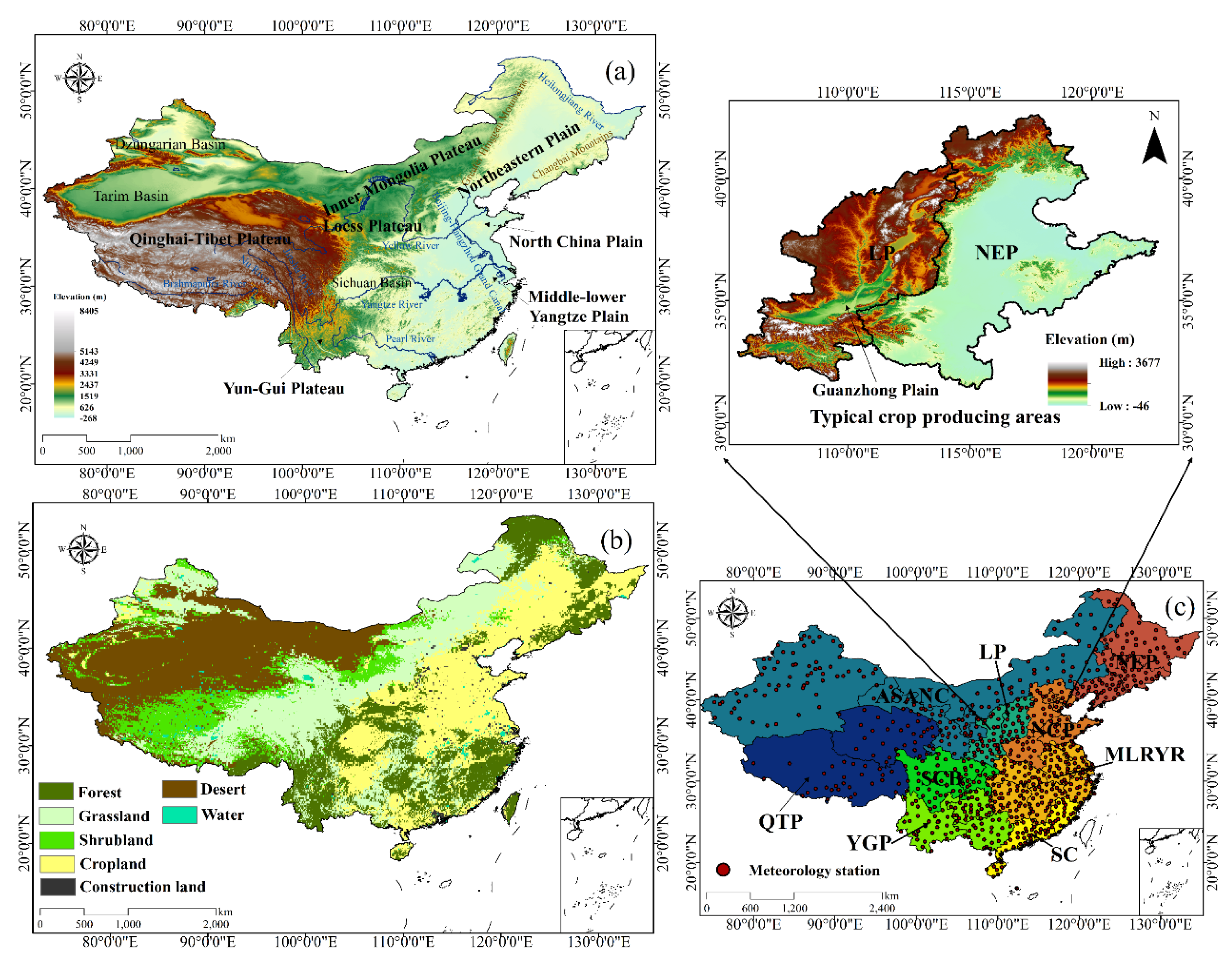
China, located in East Asia (3°51′ N−53°33′ N and 73°29′ E–135°04′ E), has an approximate land area of 9.63 × 10⁶ km2 and a sea area of 3.00 × 10⁶ km2 [14], which includes Taiwan Province and the South China Sea. As shown in Figure 1a, China has a complex terrain that mainly includes plateaus, basins, and plains. The main plateaus are the Inner Mongolia Plateau, the Loess Plateau (LP), the Qinghai–Tibet Plateau, and the Yun–Gui Plateau; the main plains are the Northeast China Plain, the NCP, and the Middle–lower Yangtze Plain; and the main basins are the Sichuan Basin, the Dzungarian Basin, and the Tarim Basin. The Yellow River, Yangtze River, and Pearl River are the main rivers in China.
Vegetation can be divided into cropland, grassland, forest, shrubland, desert, and construction land (Figure 1b). The proportion of land cover types was 23.36% cropland, 23.97% grassland, 17.97% forest, 10.31% shrubland, 23.61% desert, and 0.8% construction land in China [22,30,31]. Grassland was mainly distributed in the eastern Inner Mongolia Plateau, LP, western Qinghai–Tibet Plateau, and southern area south of the Yangtze River. Cropland was mainly distributed in the northeastern plain, NCP, Sichuan Basin, and middle–lower Yangtze Plain. Forest was mainly distributed in the Greater Khingan Mountains, Changbai Mountain, Yun–Gui Plateau, and southern middle–lower Yangtze Plain. Desert was mainly distributed in northwestern China, and shrubland was mainly distributed in the western Inner Mongolia Plateau, LP, and western Qinghai–Tibet Plateau [32,33].
Based on regional characteristics, the major crop-producing areas (croplands) were divided into nine subregions (http://www.resdc.cn/data.aspx?DATAID=275, accessed date: 21 October 2021). We named major crop-producing areas based on typical geomorphic and geographical features of major crop-producing areas. Northeast China Plain, North China Plain, Middle, and Lower Reaches of the Yangtze River, South China, Yun–Gui Plateau, Sichuan Basin sub–region, Loess Plateau, arid, and semi–arid area of North China, and Qinghai Tibet Plateau (Figure 1c). Table 1 showed the abbreviation of major crop-producing areas. The NCP and LP were defined as typical crop-producing areas in this study (Figure 1 and Figure 2).
2.2. Datasets
In this study, dynamic vegetation change was described with the Moderate Resolution Imaging Spectroradiometer (MODIS) NDVI dataset from the National Aeronautics and Space Administration (NASA) [34]. Original version data were acquired from NASA’s Earth Observing System Data and Information System Reverb (http://reverb.echo.nasa.gov/, accessed date: 21 October 2021) [35]. The temporal and spatial resolutions of this NDVI dataset were 1 month and 0.05 × 0.05, respectively. The time–series of the NDVI was from 2001 to 2017. The format of the NDVI dataset was tag image file format (TIFF) [36].
The study areas are covered by 826 meteorological stations (Figure 1c). Meteorological variables of the station included daily precipitation, temperature, wind speed, relative humidity, and atmospheric pressure. Meteorological data had a 1-day temporal resolution [37]. These meteorological data were acquired from the National Meteorological Information Centre (CMA Meteorological Data Centre) (http://data.cma.cn/en, accessed date: 21 October 2021) [10,38]. The time series of meteorological data was from 2001 to 2017. Original meteorological data were covered by the format file of text file (TXT). We employed bilinear interpolation to change the meteorological data resolution into the same as that of the NDVI dataset [39].
We used the scPDSI dataset provided by the Climatic Research Unit, University of East Anglia, UK. The scPDSI dataset has time series from 1901 to 2019. To keep the same time series with other types of dataset for this study, we select and apply time series of scPDSI from 2001 to 2017. The temporal and spatial resolution of the dataset are one month and 0.5*0.5, respectively. We also use Inverse Distance Weighted method [40] to change scPDSI spatial resolution into 0.05° × 0.05° for keeping the same resolution with NDVI dataset. For more details about the scPDSI dataset, consult van der Schrieret al. [41] (http://climexp.knmi.nl/start.cgi, accessed date: 21 October 2021).
For future metrological data, this study used the fifth phase of the Coupled Model Intercomparison Project (CMIP5) model data [10]. CMIP5 is from the Intergovernmental Panel on Climate Change (IPCC) and has different representative concentration pathway (RCP) scenarios. The RCP scenario showed different greenhouse gas emission concentrations in the future. At present, the RCP4.5 and RCP8.5 scenarios are considered closer to the actual greenhouse gas emissions than are the other RCP scenarios [10,42,43]. Therefore, the RCP4.5 and RCP8.5 scenarios were used in this study. We also defined the base period (2001–2017) and evaluation period (2020–2100) in this study. Twelve models were applied to evaluate future drought change (Table 2).
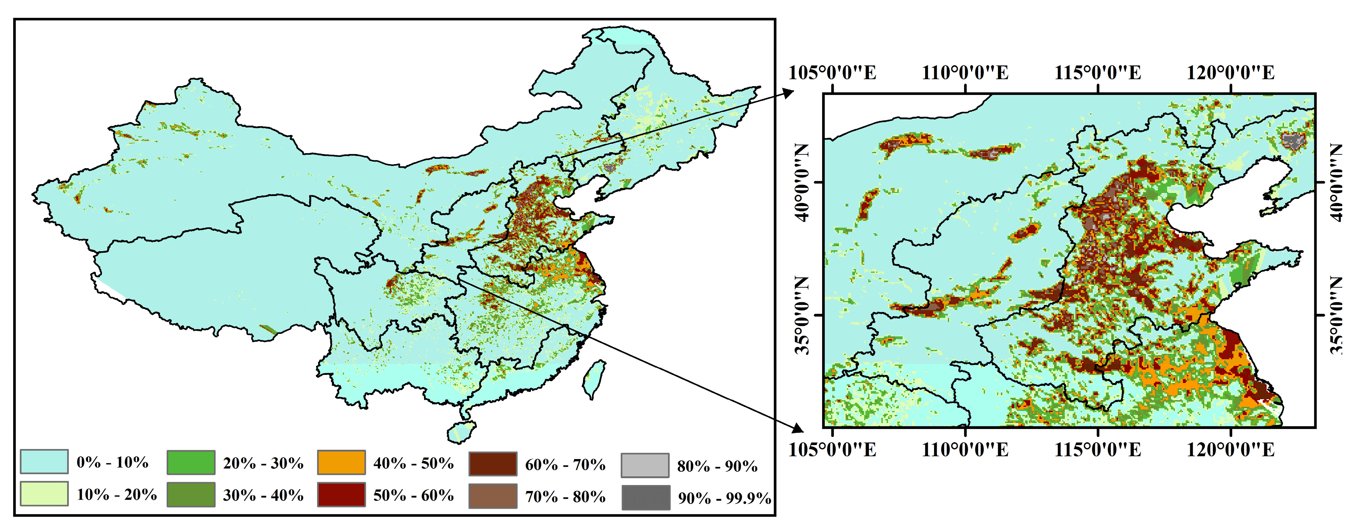
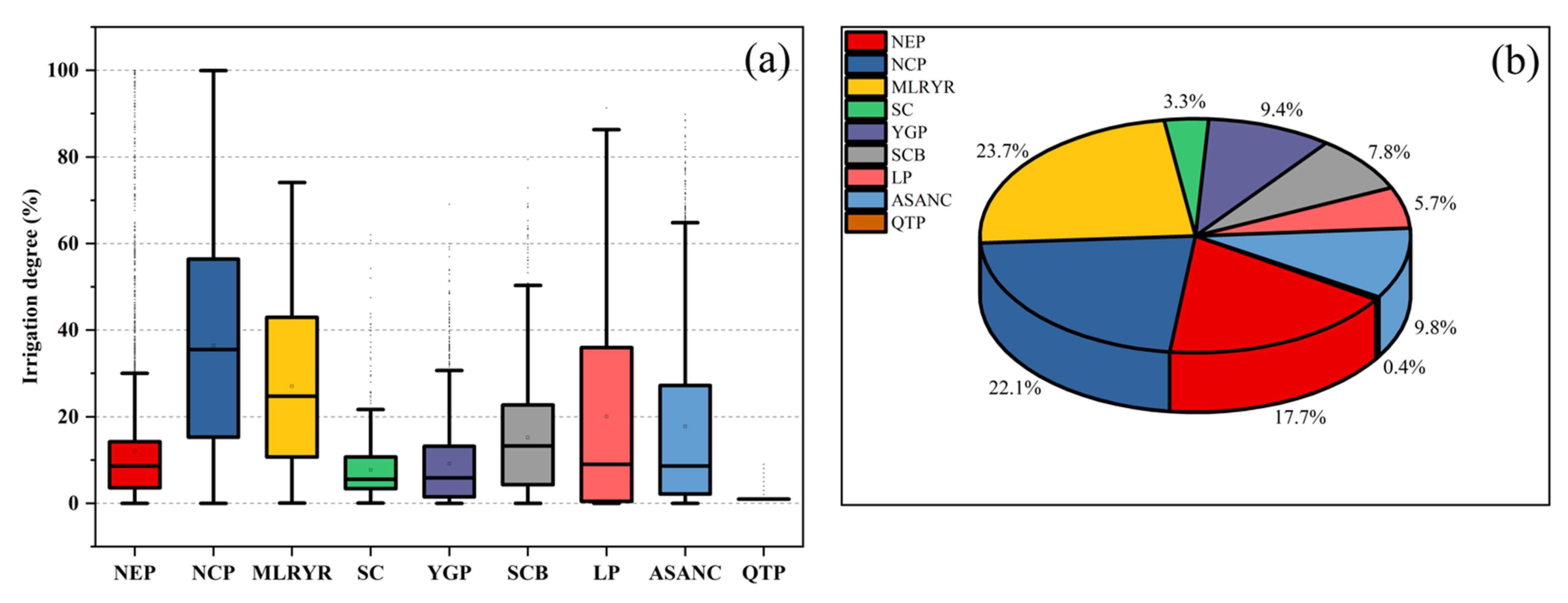
Irrigation data were obtained according to GMIA (Digital Global Map of Irrigated Area) and came from the Food and Agriculture Organization (FAO) and International Institute for Applied Systems Analysis (http://www.fao.org/soils–portal/data–hub/soil–maps–and–databases/harmonized–world–soil–database–v12/en/#jfmulticontent_c284128–3, accessed date: 21 October 2021). Irrigation data showed the global irrigation degree in 2000 [14]. The matrix of global irrigation data had 2160 lines and 4320 columns. The matrix of study area irrigation data had 567 lines and 740 columns. We employed bilinear interpolation to change the irrigation data resolution into the same as that of the NDVI dataset [39]. The irrigation degree was shown in Figure 2 and Figure 3a. As shown in Figure 2 and Figure 3a, the NCP had the highest irrigation degree, while the MLRYR and LP had higher irrigation degrees than did the other major crop-producing areas [26,31]. As shown in Figure 3b, the NCP also had the highest cropland area, while the MLRYR and NEP had higher cropland areas than did the other major crop-producing areas [32,33].
2.3. Methodology
2.3.1. Precipitation Bias Correction
Systematic biases of precipitation measurement could be caused by wetting, evaporation losses, and wind–induced under catch [48,49]. Precipitation bias correction was decreasing systematic biases of the precipitation measuring instrument by formula [37,50]. Many studies showed precipitation bias correction could significantly improve the accuracy of precipitation measurements in China [37,50]. The method for estimating corrected precipitation under standard precipitation gauge conditions in China can be found in the studies by Yang et al. [50] and Ye et al. [49].
2.3.2. Meteorological Drought SPEI
Monthly scale precipitation and potential evapotranspiration are used to calculate the SPEI. We used precipitation data of bias correction. The method of precipitation bias correction is introduced in detail in Section 2.3.1 [37]. The Penman–Monteith equation was employed to calculate the potential evapotranspiration [51,52]. Meteorological station data of precipitation and potential evapotranspiration were interpolated by the bilinear interpolation method [39] into grid cell data. The spatial resolution of the grid cell data was consistent with that of the NDVI. The drought level of the SPEI is shown in Table 3.
The calculation process of the SPEI was as follows:
where is the water deficit that can be calculated by the difference between precipitation (mm) and potential evapotranspiration (mm). The different time series of were fitted by a log–logistic probability density function to obtain the cumulative function:
where , , and are the scale, shape, and origin parameters for the values, respectively; and are the probability density function and the probability distribution function, respectively.
where is the gamma function of , and , , and are the probability weighted moments of estimated using an unbiased estimation.
when
when
where N is the chosen time scale (daily); P is the cumulative probability; C0 = 2.5155, C1 = 0.8029, C2 = 0.0103, d1 = 1.4328, d2 = 0.1893, and d3 = 0.0013.
2.3.3. Agricultural Drought scPDSI
Based on the principle of water balance, monthly scale precipitation, potential evapotranspiration, and soil moisture are used to calculate the PDSI [29,53]. Based on the hydrothermal conditions of the study area, many empirical parameters are applied in the process of calculating PDSI [14]. PDSI is processed a by self-correlation method based on the original PDSI algorithm because scPDSI can enhance the comparative performance of time and space of drought monitoring [54]. More details can be found in the studies by Dai [53], van der Schrier et al. [41], and Zhang et al. [29].
2.3.4. Modified Drought Index
The calculation process of shows a main difference between the SPEII (standardized precipitation evapotranspiration irrigation index) and the SPEI. The SPEI of considers only P and PET [55] and does not include irrigation (I). However, irrigation is an important water factor in croplands [31]. Therefore, we considered irrigation in the SPEII. The drought level of the SPEII was defined the same as that of the SPEI (Table 3).
The calculation process of SPEII was as follows:
where is the irrigation, and is the evapotranspiration. Crop coefficient () data were sufficient and reliable [56,57]. could be expressed by Equation (14). We had data for winter wheat and summer maize in typical crop-producing areas from Irrigation and Drainage Engineering [57]. However, was deficient or insufficient in most areas except in typical crop-producing areas over China. The study area of this study belongs to typical crop-producing areas and has reliable . Therefore, we used to estimated in this study.
where is the irrigation degree. When the value of is less than , the value is equal to ; when the value of is more than , the value is equal to 0.
indicates that human activity provides some water (from the stream and groundwater) to cropland based on the natural water deficit (P minus PET) from the stream and groundwater. If the natural water deficit is less than 0, the irrigation degree can be expressed by the supplementary partial natural water deficit; otherwise, if the natural water deficit is more than 0, the natural water deficit is sufficient, and it is not necessary to irrigate cropland. Monthly irrigation was computed in this study. When there is less irrigation or other types of land (such as grassland and forest), the water deficit is very close to the difference between precipitation and potential evapotranspiration. The irrigation level was considered as similar in different regions of China. Meanwhile, the grid cells were considered as a unit in this study. Therefore, the irrigation degree was considered as an irrigation water amount in cropland in a grid-cell unit [57]. Yet the actually irrigated area was different from equipped for irrigation area because the advanced level of irrigation equipment is not completely consistent in China of different regions. Then, the SPEII is also close to the SPEI. We do not introduce the standardization process again because the SPEII is the same as the SPEI in the subsequent standardization process. The irrigation degree data were from the FAO. We tested the applicability of log–logistic fitting in the SPEII. The result showed acceptable applicability of log–logistic fitting in the SPEII. We used the Savitzky-Golay method to smooth the SPEII data [3]. The trend line of the SPEI1 can show the change characteristics of drought. The Savitzky-Golay method was also used to smooth drought [3] and runoff [58] data.
2.3.5. Vegetation Response Degree and Time to Drought
The vegetation response to drought was quantitated by the Pearson correlation coefficient (p < 0.05) between the NDVI and drought index [59,60]. We calculated different time-scales of the SPEI and SPEII [24]. Different time-scaled SPEIIs and SPEIs were labeled SPEIIn and SPEIn, where n represents the time scale. The correlation coefficient of different time-scales (1 to 12 months) was also calculated between the drought indexes and NDVI. The response degree of vegetation to drought was defined as the time scale (1 to 12 months) of the correlation coefficient of the maximum absolute value. The response time of vegetation to drought was defined as the time scale of the correlation coefficient of the maximum absolute value between 1 and 12 on the monthly time scale [15,61]. The response degree of summer maize and winter wheat to drought was shown by the correlation coefficient in the crop growth period over typical crop-producing areas. The crop growth period of summer maize and winter wheat was defined as being from late June to early September and from late September to early June of the following year, respectively [62,63].
3. Results
3.1. Comparing the Applicability between Traditional Drought Indexes and SPEII
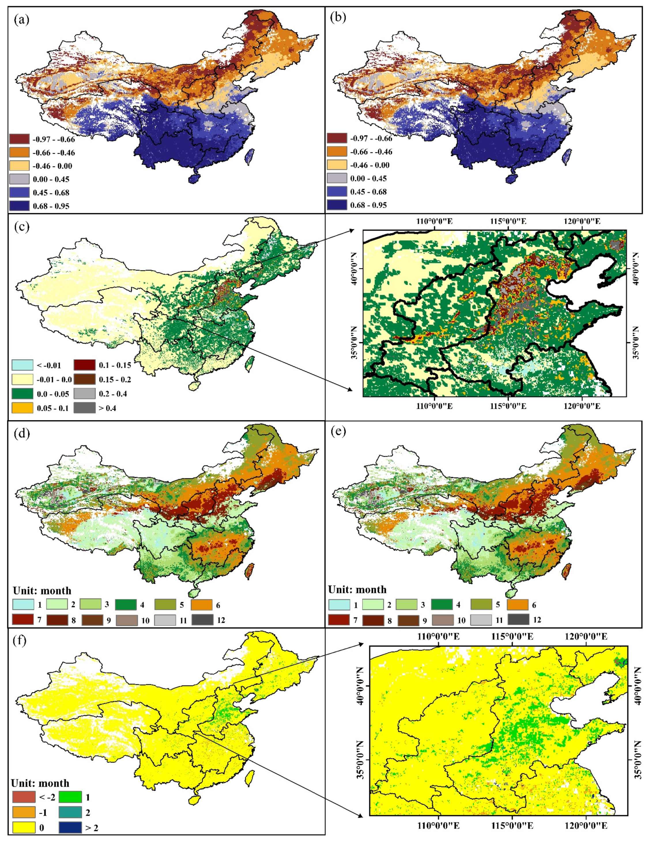
From Figure 4a,b, we found that vegetation showed a similar response degree to the SPEII (Figure 4a) and the SPEI (Figure 4b). Northern China (NEP, NCP, LP and ASANC) showed a generally negative response to drought, while southern China (MLRYR, YGP, SC, QTP and SCB) showed a generally positive response to drought. Comparing Figure 2 and Figure 4c, we found that positive correlation coefficient difference values showed close spatial distribution to the irrigation degree. Positive correlation coefficient difference values were distributed mainly in eastern China’s Dzungarian Basin and the Tarim Basin. Meanwhile, Figure 4c showed that the SPEII mainly had higher correlation coefficient areas than SPEI in eastern China. However, SPEI mainly had higher correlation coefficient than SPEII in western China. Meanwhile, the correlation coefficient difference had 37.1%, 10.5% and 52.3% areas more than 0, less than 0, and equal to 0, respectively. Only 0.35% of the correlation coefficient difference areas were less than −0.01. By comparing Figure 3 and Figure 4c, we found that SPEII had higher correlation coefficient than SPEI in irrigation area of China. However, SPEII had lower correlation coefficient than SPEI in non-irrigation area of China.
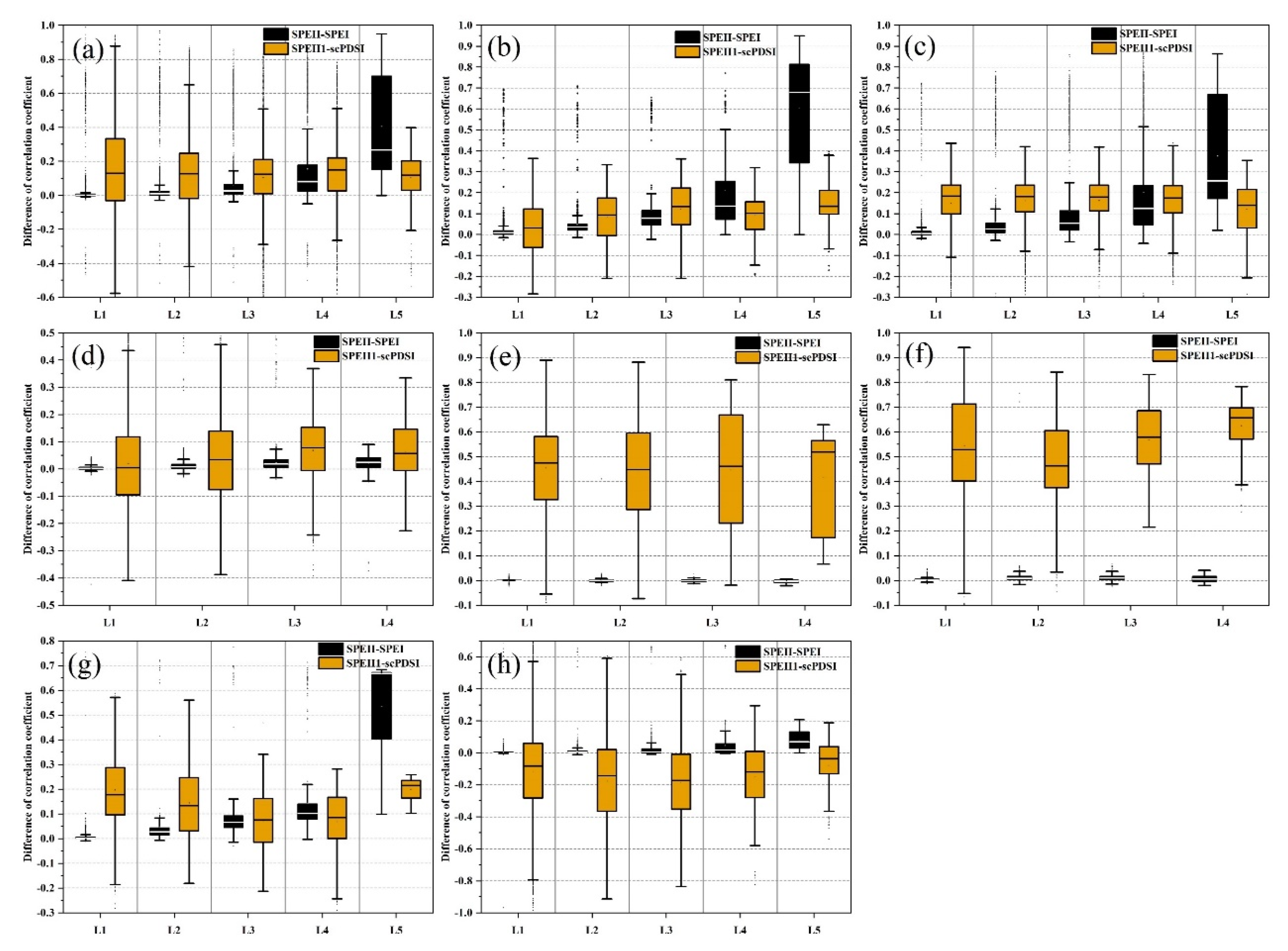
Additionally, the size of the positive correlation coefficient difference values in typical crop-producing areas was closely spatially distributed to the irrigation level. We can speculate that the size of the positive correlation coefficient difference values might be related to the level of irrigation. Therefore, Figure 5 could help to analyze the relationship between the size of the positive correlation coefficient difference values and the level of irrigation degree. We did not consider the SC and QTP major crop-producing areas in Figure 5 because of the lower irrigation and smaller cropland areas in SC and QTP. We compared the difference between SPEII1 and scPDSI because scPDSI just had 1 month time scale in calculation [14].
In general, the size of the difference values of the correlation coefficient between SPEII and SPEI obviously had increased with increasing irrigation degree in China, NEP, NCP, MLRYR, LP, and ASANC (Figure 5). The difference values of the correlation coefficient between SPEII and SPEI showed similar level in different irrigation degree in YGP (range ≈ −0.01–0) and SCB (range ≈ 0–0.04). Meanwhile, in general, the difference of the correlation coefficient between SPEII and SPEI is positive values. The correlation coefficient difference values between SPEII1 and scPDSI showed similar level in different irrigation degree. However, the correlation coefficient difference values between SPEII1 and scPDSI showed different level in different major crop-producing areas. Accordingly, the correlation coefficient difference values between SPEII1 and scPDSI reached a higher level in YGP (range ≈ 0.20–0.65) and SCB (range ≈ 0.40–0.70). The correlation coefficient difference values between SPEII1 and scPDSI had lower level in China (range ≈ 0–0.30), NEP (range ≈ −0.10–0.20), NCP (range ≈ 0–0.25), MLRYR (range ≈ −0.10–0.15), and LP (range ≈ 0–0.30). However, the correlation coefficient difference between SPEII1 and scPDSI, generally, had negative values in ASANC (range ≈ −0.40–0). Based on Figure 4 and Figure 5, we found that the SPEII showed a higher correlation with the NDVI than did the SPEI in irrigated cropland. The SPEII showed more significant advantages than the SPEI in monitoring drought in cropland vegetation fields with high irrigation levels. SPEII had higher correlation with the NDVI than did the scPDSI in irrigated cropland (except ASANC). Therefore, in general, SPEII also had more excellent performance than scPDSI in monitoring drought in cropland vegetation fields.
From Figure 4d,e, we found that vegetation showed similar response times to the SPEII (Figure 4a) and SPEI (Figure 4b). The response time of vegetation to the drought main range was 5 to 8 months in northeastern China, the Inner Mongolia Plateau, and the middle–lower Yangtze Plain. The response time in the main range was 1 to 4 months in southwestern and northwestern China. The response time range was 6 to 7 and 2 to 3 months in the northern and southern NCP, respectively. From Figure 2 and Figure 4f, we found that the vegetation response time to the SPEII was more than 1 month different than that of the SPEI in large-area irrigation croplands. Therefore, the SPEII also showed a longer response time of vegetation than the SPEI in irrigated cropland. We summed the area with a difference in response time greater than 0 at different irrigation levels (L1, L2, L3, L4, and L5). The proportion of this area to the total irrigation area at different levels was 2.70%, 8.35%, 17.2%, 39.9%, and 60.6%, respectively. Based on statistical analysis, we found that the proportion of the area with a response time difference greater than 0 increased with the improvement in irrigation level. Therefore, the SPEII showed a significantly longer vegetation response time than the SPEI in cropland with a high irrigation level.
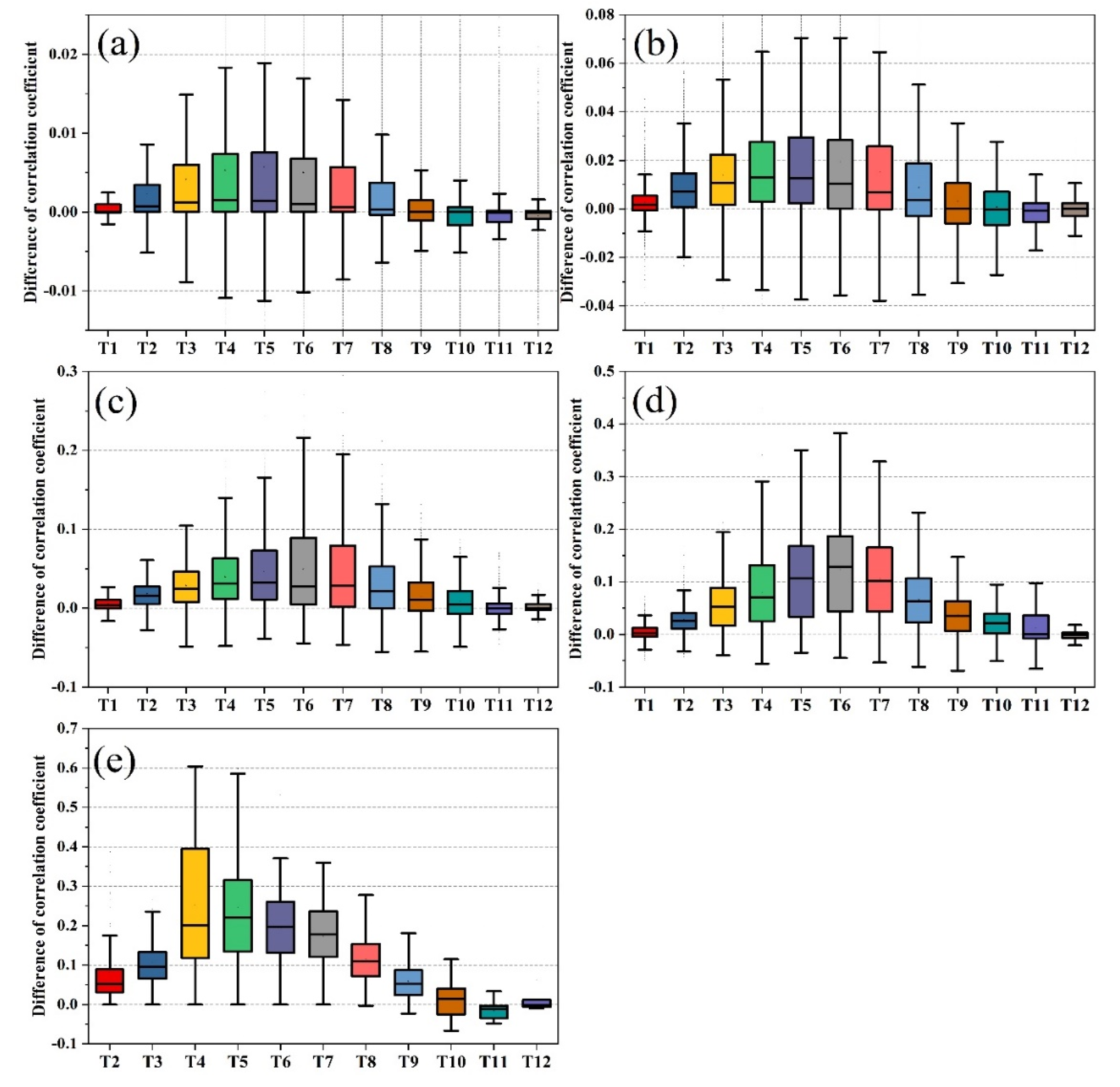
Different time scales of correlation coefficient difference values were summed in croplands with different irrigation levels (Figure 6). From Figure 6, we found that the time scales of 5, 6, and 7 months had higher correlation coefficient difference values than did the other time scales at different irrigation levels. Therefore, SPEII5, SPEII6, and SPEII7 showed greater performance than SPEI5, SPEI6, and SPEI7 in monitoring vegetation drought. Meanwhile, the correlation coefficient differences at the different irrigation levels mainly ranged from 0 to 0.01 (Figure 6a), 0 to 0.03 (Figure 6b), 0 to 0.10 (Figure 6c), 0 to 0.20 (Figure 6d), and -0.05 to 0.40 (Figure 6e). Therefore, the high irrigation level of the SPEII showed a more significant advantage than that of the SPEI at different time scales.
3.2. Assessing the Applicability of the SPEII in Typical Crop-Producing Areas
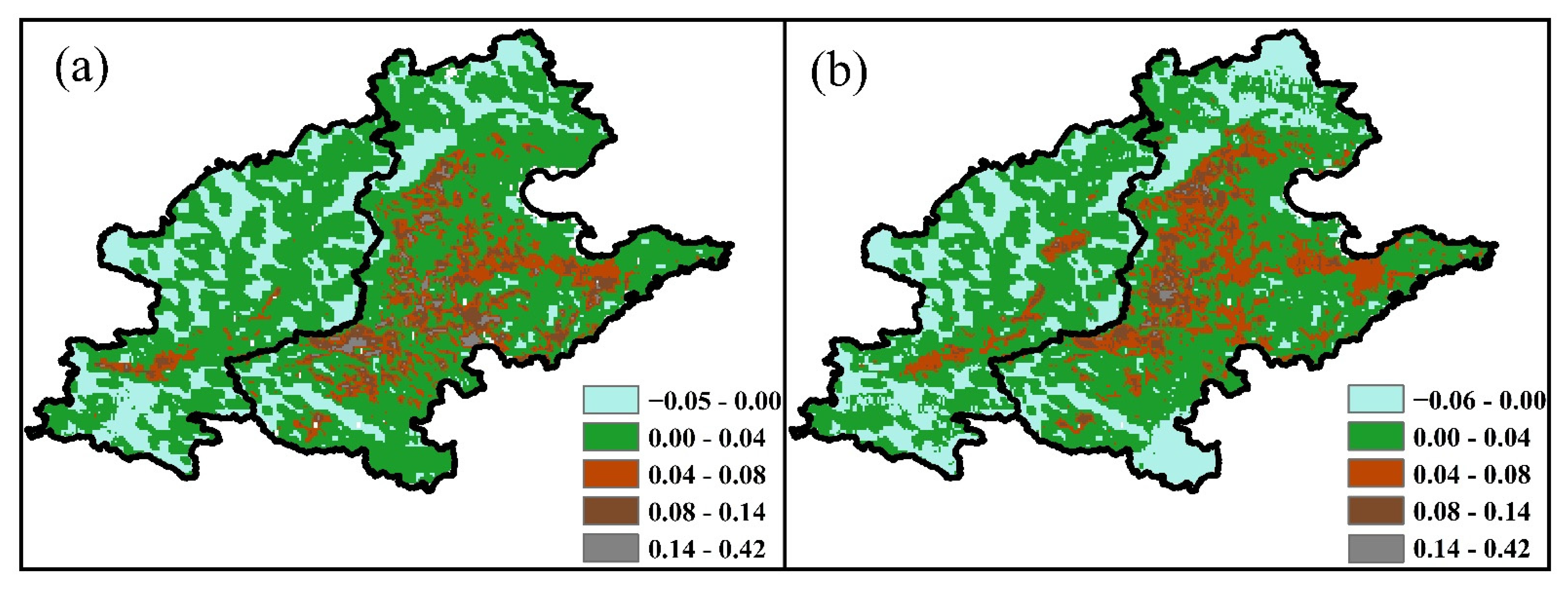
Considering the crop coefficient of winter wheat and summer maize [56], we acquired the actual evapotranspiration of crops in the NCP and LP. We could correctly assess the performance of the SPEII and SPEI by the actual evapotranspiration of crops. From Figure 7, we found that the correlation coefficient difference of both winter wheat and summer maize showed positive values and closed spatial distribution characteristics with irrigation (Figure 2). Therefore, the SPEII had a better performance than the SPEI in the growth periods of winter wheat and summer maize.
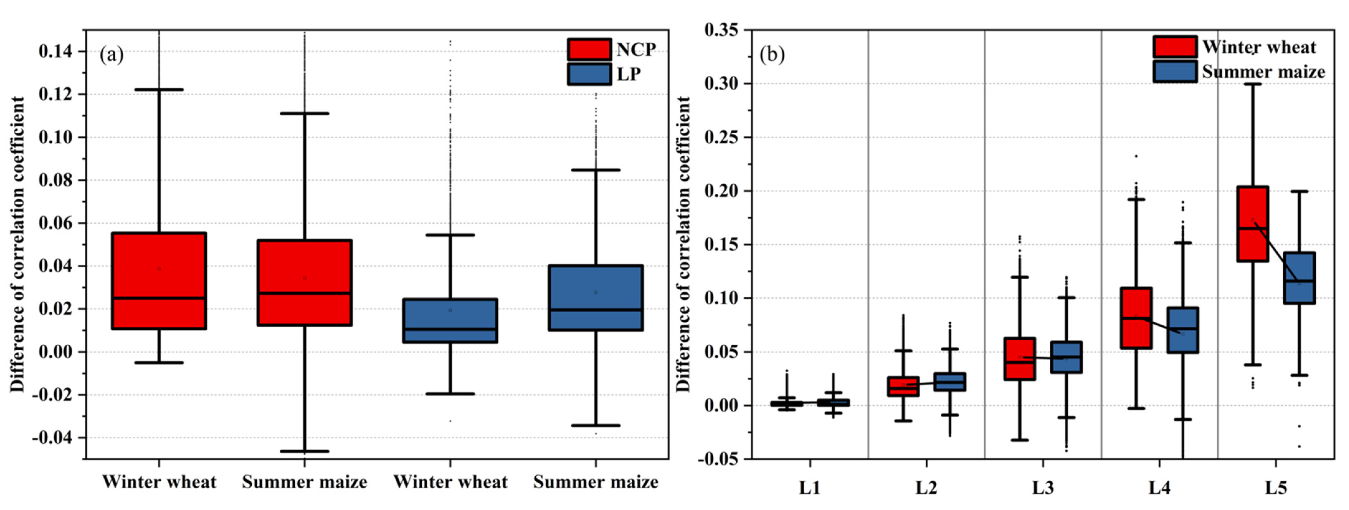
From Figure 8a, winter wheat had main ranges from 0.01 to 0.05 and 0 to 0.02 in the NCP and LP, respectively. Summer maize had main ranges from 0.01 to 0.05 and 0.01 to 0.04 in the NCP and LP, respectively. Therefore, the NCP showed a higher correlation coefficient difference than the LP in the growth period. However, both winter wheat and summer maize had similar correlation coefficient differences in typical crop-producing areas. From Figure 8b, the correlation coefficient difference of the winter wheat main range was from 0.01 to 0.03, 0.02 to 0.06, 0.05 to 0.11 and 0.14 to 0.21 in L2, L3, L4, and L5, respectively. Meanwhile, the correlation coefficient difference of the summer maize main range was from 0.01 to 0.03, 0.03 to 0.06, 0.05 to 0.09 and 0.1 to 0.14 in L2, L3, L4, and L5, respectively. The difference in the correlation coefficient of both winter wheat and summer maize increased with increasing irrigation level. Therefore, the SPEII showed greater performance than the SPEI in monitoring drought in winter wheat and summer maize. However, winter wheat showed a higher correlation coefficient difference than summer maize. The SPEII might have greater performance in monitoring winter wheat than summer maize in the NCP and LP.
3.3. Drought Change under Different Scenarios in the Future
Considering the CMIP5 model of the RCP4.5 and RCP8.5 scenarios, we evaluated drought changes in winter wheat and summer maize in the growth period in the future. From Figure 9a,b, we found that drought did not show a significant change between the base period and the future. Under the RCP4.5 scenario, the winter wheat growth-period SPEII values showed slightly higher levels in 2020–2039 and 2060–2079 (Figure 9a). The winter wheat growth-period drought showed a decreasing trend in 2030–2045 and 2070–2080 and an increasing trend in 2050–2060 and 2080–2100 (Figure 9c). Under the RCP8.5 scenario, the winter wheat SPEII value was slightly lower in 2040–2059, 2060–2079 and 2080–2100 (Figure 9a). The winter wheat under growth-period drought showed a decreasing trend in 2020–2080 and 2090–2099 and an increasing trend in 2080–2090 (Figure 9c). Under the RCP4.5 scenario, the summer maize of the growth period showed similar SPEII values in the base period and future periods (Figure 9b). The summer maize of the growth-period drought showed a decreased trend in 2050–2065, 2075–2080 and 2090–2100 and an increased trend in 2030–2050, 2065–2075 and 2080–2090 (Figure 9d). Under the RCP8.5 scenario, the summer maize of the growth-period SPEII value was slightly lower in 2040–2059 and 2060–2079 (Figure 9b). However, the drought trend was steady between 2020 and 2100 in summer maize during the growth period (Figure 9d).
From Figure 10, under the RCP4.5 and RCP8.5 scenarios, moderate and severe drought had a higher frequency than extreme drought in the NCP. However, drought frequency from high to low was severe, moderate, and extreme in the LP, respectively. Under the RCP4.5 scenario, the frequencies of moderate, severe and extreme drought were distributed mainly from 0.12 to 0.17, 0.1 to 0.16 and 0.1 to 0.13 in the NCP, respectively. However, extreme drought showed a higher frequency in 2060–2079 over the NCP (Figure 10a). Under the RCP8.5 scenario, the frequencies of moderate, severe, and extreme drought were distributed mainly from 0.11 to 0.17, 0.1 to 0.16 and 0.09 to 0.13 in the NCP, respectively (Figure 10c). Under the RCP4.5 scenario, the frequencies of moderate, severe, and extreme drought were distributed mainly from 0.13 to 0.16, 0.16 to 0.21 and 0.1 to 0.13 in the LP, respectively (Figure 10b). However, moderate drought had higher and lower frequencies in the base period and in 2040–2059 over the LP, respectively. Severe drought had a lower frequency in the base period over the LP. Extreme drought had a higher and lower frequency in 2060–2079 and in the base period over the LP, respectively. Under the RCP8.5 scenario, the frequencies of moderate, severe, and extreme drought were distributed mainly from 0.1 to 0.16, 0.15 to 0.21 and 0.09 to 0.13 in the LP, respectively (Figure 10d). However, moderate drought had a higher frequency in the base period and in 2080–2100 over the LP. Severe drought showed higher and lower frequencies in 2020–2039 and in 2060–2079 over the LP, respectively. Extreme drought showed a lower frequency in the base period and in 2080–2100 over the LP.
Examining Section 3.1, we found that the SPEII6 showed greater performance than the other time-scale SPEIIs in monitoring the vegetation response to drought (Figure 6). Therefore, based on the CMIP5 model, we used the SPEII6 to evaluate future drought in the NCP and LP. From Figure 11, we found that a higher frequency of moderate drought was distributed mainly in the southeastern NCP and in the Guanzhong Plain of the LP. A higher frequency of severe drought was distributed mainly in the northern NCP as well as in the northern and southern LP. However, the NCP and LP showed a lower frequency of extreme drought.
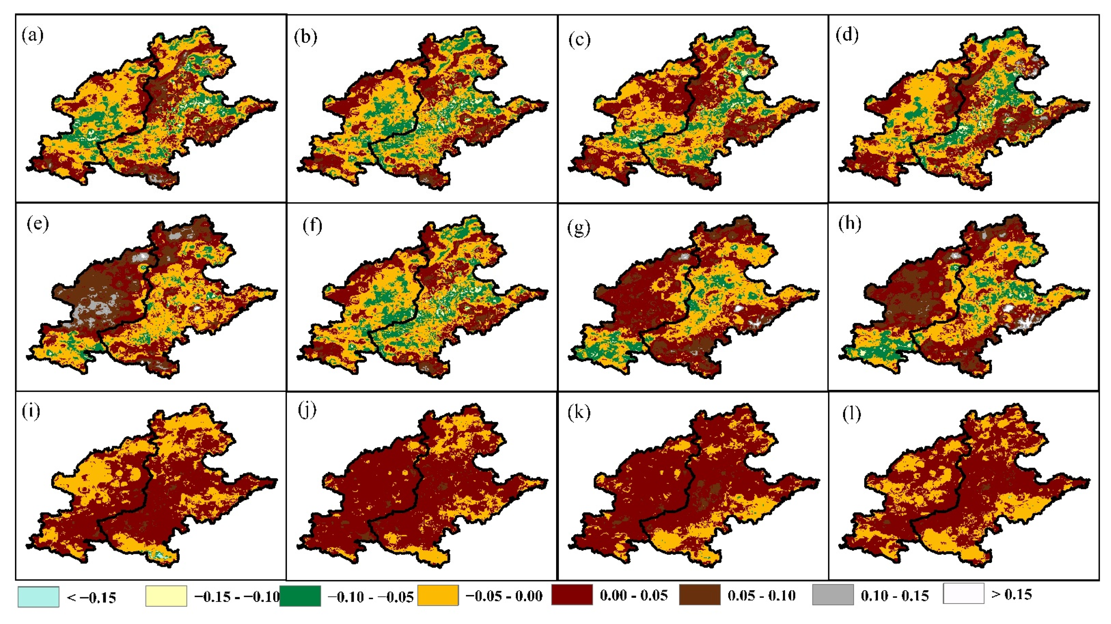
From Figure 12a–d, relative to the base period, the frequency of moderate drought showed a decreasing trend in the southern NCP and central LP under the RCP4.5 scenario. From Figure 12e–h, relative to the base period, the frequency of moderate drought showed a decreasing trend in the northern NCP and southern LP. The frequency of moderate drought showed an increasing trend in the northern NCP and central LP. Moreover, the frequency of moderate drought in the central LP showed a significant increase in 2040–2059. From Figure 12i–l, relative to the base period, the frequency of extreme drought showed a slight increase in larger areas of the NCP and LP; moreover, the frequency of extreme drought in the southeastern NCP showed a significant increase in 2060–2079. From Figure 13a–d, relative to the base period, the frequency of moderate drought showed a decreasing trend in the southern and central NCP and the central LP. From Figure 13e–h, relative to the base period, the frequency of moderate drought showed a decreasing trend in the northern and central NCP and the southern LP. The frequency of moderate drought showed a decreasing trend in the central NCP and southern LP. The frequency of moderate drought showed an increasing trend in the southeastern NCP and northern and central LP; moreover, moderate drought frequency in the central and northern LP had significant increases in 2020–2039. From Figure 12i,g–l, relative to the base period, the frequency of extreme drought showed a slight increase in larger areas of the NCP and LP.
4. Discussion
4.1. Advantages and Disadvantages of Improving the Drought Index
Examining Section 3.1 and Section 3.2, we compared the performance between the SPEII and SPEI in monitoring vegetation drought. The results showed that the SPEII generally had a greater performance than the SPEI in monitoring vegetation drought in cropland with a high irrigation level. Many studies have found that vegetation growth is impacted mainly by the natural climate [15] and human activity [9,64]. However, the SPEI considers the precipitation and evapotranspiration of natural meteorological factors and ignores the irrigation factors of human activity [14,55]. In this study, the SPEII considered the irrigation factor of human activity to improve the ability to monitor cropland drought [65]. From Figure 2, the NCP, MLRYR, LP, and ASANC showed higher irrigation degrees [26,31]. However, the SPEII did not show significant advantages in the ASANC and MLRYR (Figure 4 and Figure 5). The SPEII also showed significant advantages in the NEP and SCB with general irrigation levels. The water use efficiency of irrigation also impacted cropland drought and the SPEII performance [31]. Water use efficiency is defined as the degree of effective irrigation water use by crops [25,31]. The water use efficiency of irrigation is mainly impacted by irrigation strategies and soil properties [25]. Poor irrigation strategies and loose soil properties could lead to evapotranspiration and deep percolation of irrigation water with low water use efficiency in croplands [25]. The study by Li et al. [31] found that the MLRYR and ASANC had lower irrigation water use efficiency. The NEP and NCP had higher irrigation water use efficiency [31]. Although the MLRYR and ASANC had higher irrigation levels, crops poorly effectively used irrigation water in the MLRYR and ASANC [27]. Therefore, the poorer performance of the SPEII could be impacted by the lower water use efficiency of irrigation in the MLRYR and ASANC [31]. Moreover, the water use efficiency of irrigation could be improved by rational planning of irrigation strategies and changing soil structure characteristics [25,31]. Based on the same principle, the NEP also had a higher irrigation water use efficiency, which could lead to greater performance [26]. The SPEII also showed that crop vegetation had a longer response time to drought in the NCP and LP. Irrigation could slow the time of crop vegetation response to meteorological drought [3,23]. Therefore, the SPEII showed a more accurate response time to drought in croplands with high irrigation levels. The SPEII also had an extensive application foundation advantage because we considered two cases of evapotranspiration calculations of sufficient and insufficient crop coefficient data [56].
However, the SPEII also has some disadvantages in application. The accuracy of evapotranspiration [51] and irrigation [62] might impact the SPEII performance in monitoring vegetation drought. We estimated cropland irrigation by water deficit and irrigation degree. Actual irrigation might not be equal to theoretical irrigation [62]. Actual evapotranspiration of crops can also be replaced by potential evapotranspiration when crop coefficient data are insufficient [51]. Crop coefficients and actual irrigation data are hard to obtain in studies [31,56]. Therefore, we have to increase the extensive application of the SPEII at the expense of accuracy. Moreover, we found that the SPEII showed poorer performance than the SPEI in monitoring the drought of cropland vegetation on the YGP (Figure 5e). From Figure 1c and Figure 2, we found that cropland in irrigation areas showed spatially discrete distribution characteristics. Zhou et al. [66] and Ding et al. [22] also found that cropland vegetation was impacted by the ecological environment because a healthy ecological environment structure had strong resistance to drought change. Therefore, the SPEII showed the same performance of monitoring drought as the SPEI in cropland that was spatially discrete and had a healthy ecological environment structure.
4.2. Irrigation Strategies to Address Future Drought
Based on previous studies, the NCP lacks agricultural water resources and maintains a high irrigation level [22,26,61,67]. Therefore, irrigation might implement a spatiotemporal irrigation strategy to respond to climate change in the future when the NCP is unable to significantly improve the irrigation level [31,63]. Examining Section 3.3, we found that the winter wheat growth period showed a trend of increasing drought degree in 2020–2080 under the RCP8.5 scenario (Figure 9). However, the summer maize of the growth period showed a steady trend of drought change in 2020–2100 (Figure 9). Therefore, we could adjust the irrigation guarantee level between the winter wheat and summer maize growth periods in the future [67]. Given the possibility of drought change in the future, the strategic scheduling of water resources should be implemented to ensure the global optimum of water resource allocation in typical crop-producing areas [28,68]. Examining Section 3.3, we also found that moderate drought had a decreased frequency in the central NCP and extreme drought had an increased frequency in the southeastern NCP in the future (Figure 12). The severe drought frequency showed an increase in 2020–2039 over the central LP (Figure 13). Therefore, we might consider scheduling water resources from the central to the southeastern NCP in 2060–2079. Moreover, we might consider scheduling water resources from the central NCP to the central LP in 2020–2039.
5. Conclusions
In this study, we investigated the performance of the SPEII in monitoring cropland vegetation drought and evaluating regional drought changes in the future. Correlation analysis, comparison analysis, and grid-cell mapping, in addition to CMIP5 models, were applied to evaluate drought change-based SEPII. The results can provide reference for agricultural drought early warning and monitoring in the future. The main conclusions were as follows:
- (1)
- In general, the SPEII had better performance than SPEI and scPDSI in monitoring cropland vegetation drought because traditional drought indexes consider irrigation caused by human activity in China. The SPEII showed more significant performance in cropland with a higher irrigation level than in cropland with a lower irrigation level in China, in general. The SPEII5, SPEII6, and SPEII7 had more significant performance than did the other time scales of the SPEII.
- (2)
- The SPEII in typical crop-producing areas (NCP and LP) also had excellent performance compared with the SPEI on both different time scales and crop (winter wheat and summer maize) growth periods. The SPEII on the NCP showed better performance than that on the LP in both the winter wheat and the summer maize growth periods. The winter wheat growth period of the SPEII had better performance than that of the summer maize in areas with higher irrigation levels in typical crop-producing areas.
- (3)
- In general, future drought showed a similar drought degree with the base period (2001–2007) in typical crop-producing areas. The drought degree of winter wheat and summer maize growth periods showed increasing and steady trends in 2020–2080 under the RCP4.5 scenario in the future, respectively. In the future, extreme drought frequency in the southeastern NCP will increase between 2060 and 2079; severe drought frequency in the central LP will increase between 2020 and 2059. The moderate drought frequency in the central NCP will decrease in the future.
Author Contributions
Conceptualization, L.H. and Y.D. (Yibo Ding); methodology, L.H.; software, L.T.; validation, Z.Z., L.H. and T.G.; formal analysis, L.T.; investigation, Y.D. (Yibo Ding); resources, Y.D. (Yanan Ding); data curation, Z.Z.; writing original draft preparation, L.H.; writing review and editing, Z.Z.; visualization, Y.Z.; project administration, W.F.; funding acquisition, Liupeng He. All authors have read and agreed to the published version of the manuscript.
Funding
This study was funded by major projects of a high-resolution earth observation system (80-H30G03-9001-20/22). This subtopic (80-H30G03-9001-20/22) was from the special scientific research projects (civil part) of the high-resolution Earth observation system. Dynamic monitoring and evaluation of regional agricultural water saving level based on multi-source remote sensing information (Major key technology research project of water conservancy in 2021).
Informed Consent Statement
Informed consent was obtained from all subjects involved in the study.
Conflicts of Interest
The authors declare no conflict of interest.
References
- Huang, S.; Huang, Q.; Chang, J.; Zhu, Y.; Leng, G.; Xing, L. Drought structure based on a nonparametric multivariate standardized drought index across the Yellow River basin, China. J. Hydrol. 2015, 530, 127–136. [Google Scholar] [CrossRef]
- Mishra, A.K.; Singh, V.P. A review of drought concepts. J. Hydrol. 2010, 391, 202–216. [Google Scholar] [CrossRef]
- Wan, W.; Liu, Z.; Li, K.; Wang, G.; Wu, H.; Wang, Q. Drought monitoring of the maize planting areas in Northeast and North China Plain. Agric. Water Manag. 2021, 245, 106636. [Google Scholar] [CrossRef]
- Shao, Y.; Zhang, Y.; Wu, X.; Bourque, C.P.A.; Zhang, J.; Qin, S.; Wu, B. Relating historical vegetation cover to aridity patterns in the greater desert region of northern China: Implications to planned and existing restoration projects. Ecol. Indic. 2018, 89, 528–537. [Google Scholar] [CrossRef]
- Wilhite, D.A.; Svoboda, M.D.; Hayes, M.J. Understanding the complex impacts of drought: A key to enhancing drought mitigation and preparedness. Water Resour. Manag. 2007, 21, 763–774. [Google Scholar] [CrossRef] [Green Version]
- Shi, H.; Chen, J.; Wang, K.; Niu, J. A new method and a new index for identifying socioeconomic drought events under climate change: A case study of the East River basin in China. Sci. Total Environ. 2018, 616, 363–375. [Google Scholar] [CrossRef] [PubMed] [Green Version]
- Faiz, M.A.; Liu, D.; Fu, Q.; Li, M.; Baig, F.; Tahir, A.A.; Khan, M.I.; Li, T.; Cui, S. Performance evaluation of hydrological models using ensemble of General Circulation Models in the northeastern China. J. Hydrol. 2018, 565, 599–613. [Google Scholar] [CrossRef]
- Dufresne, J.L.; Foujols, M.A.; Denvil, S.; Caubel, A.; Marti, O.; Aumont, O.; Balkanski, Y.; Bekki, S.; Bellenger, H.; Benshila, R.; et al. Climate change projections using the IPSL-CM5 Earth System Model: From CMIP3 to CMIP5. Clim. Dyn. 2013, 40, 2123–2165. [Google Scholar] [CrossRef]
- Shi, Y.; Jin, N.; Ma, X.; Wu, B.; He, Q.; Yue, C.; Yu, Q. Attribution of climate and human activities to vegetation change in China using machine learning techniques. Agric. For. Meteorol. 2020, 294, 108146. [Google Scholar] [CrossRef]
- Zhou, Z.Q.; Ding, Y.B.; Shi, H.Y.; Cai, H.J.; Fu, Q.; Liu, S.N.; Li, T.X. Analysis and prediction of vegetation dynamic changes in China: Past, present and future. Ecol. Indic. 2020, 117, 11. [Google Scholar] [CrossRef]
- Zadeh, N.; Yin, J.; Wyman, B.L.; Wittenberg, A.T.; Samuels, B.L.; Palter, J.B.; Liang, Z.; Lee, H.-C.; Hurlin, W.J.; Gnanadesikan, A.; et al. The GFDL CM3 Coupled Climate Model: Characteristics of the Ocean and Sea Ice Simulations. J. Clim. 2011, 24, 3520–3544. [Google Scholar]
- Nourani, V.; Baghanam, A.H.; Gokcekus, H. Data-driven ensemble model to statistically downscale rainfall using nonlinear predictor screening approach. J. Hydrol. 2018, 565, 538–551. [Google Scholar] [CrossRef]
- Wu, C.; Yeh, P.J.F.; Chen, Y.-Y.; Lv, W.; Hu, B.X.; Huang, G. Copula-based risk evaluation of global meteorological drought in the 21st century based on CMIP5 multi-model ensemble projections. J. Hydrol. 2021, 598, 126265. [Google Scholar] [CrossRef]
- Ding, Y.; Gong, X.; Xing, Z.; Cai, H.; Zhou, Z.; Zhang, D.; Sun, P.; Shi, H. Attribution of meteorological, hydrological and agricultural drought propagation in different climatic regions of China. Agric. Water Manag. 2021, 255, 106996. [Google Scholar] [CrossRef]
- Zhou, Z.; Shi, H.; Fu, Q.; Ding, Y.; Li, T.; Wang, Y.; Liu, S. Characteristics of propagation from meteorological drought to hydrological drought in the Pearl River Basin. J. Geophys. Res. Atmos. 2021, 126, e2020JD033959. [Google Scholar] [CrossRef]
- Jiang, T.; Su, X.; Singh, V.P.; Zhang, G. A novel index for ecological drought monitoring based on ecological water deficit. Ecol. Indic. 2021, 129, 107804. [Google Scholar] [CrossRef]
- Wang, F.; Wang, Z.; Yang, H.; Di, D.; Zhao, Y.; Liang, Q. A new copula-based standardized precipitation evapotranspiration streamflow index for drought monitoring. J. Hydrol. 2020, 585, 124793. [Google Scholar] [CrossRef]
- Jiao, W.; Wang, L.; Novick, K.A.; Chang, Q. A new station-enabled multi-sensor integrated index for drought monitoring. J. Hydrol. 2019, 574, 169–180. [Google Scholar] [CrossRef]
- Wang, L.; Yu, H.; Yang, M.; Yang, R.; Gao, R.; Wang, Y. A drought index: The standardized precipitation evapotranspiration runoff index. J. Hydrol. 2019, 571, 651–668. [Google Scholar] [CrossRef]
- Wu, D.; Li, Z.; Zhu, Y.; Li, X.; Wu, Y.; Fang, S. A new agricultural drought index for monitoring the water stress of winter wheat. Agric. Water Manag. 2021, 244, 106599. [Google Scholar] [CrossRef]
- Won, J.; Choi, J.; Lee, O.; Kim, S. Copula-based Joint Drought Index using SPI and EDDI and its application to climate change. Sci. Total Environ. 2020, 744, 140701. [Google Scholar] [CrossRef] [PubMed]
- Ding, Y.; Xu, J.; Wang, X.; Peng, X.; Cai, H. Spatial and temporal effects of drought on Chinese vegetation under different coverage levels. Sci. Total Environ. 2020, 716, 137166. [Google Scholar] [CrossRef] [PubMed]
- Kong, D.; Miao, C.; Wu, J.; Zheng, H.; Wu, S. Time lag of vegetation growth on the Loess Plateau in response to climate factors: Estimation, distribution, and influence. Sci. Total Environ. 2020, 744, 140726. [Google Scholar] [CrossRef]
- Xu, H.-J.; Wang, X.-P.; Zhao, C.-Y.; Yang, X.-M. Diverse responses of vegetation growth to meteorological drought across climate zones and land biomes in northern China from 1981 to 2014. Agric. For. Meteorol. 2018, 262, 1–13. [Google Scholar] [CrossRef]
- Li, X.; Zhao, W.; Li, J.; Li, Y. Effects of irrigation strategies and soil properties on the characteristics of deep percolation and crop water requirements for a variable rate irrigation system. Agric. Water Manag. 2021, 257, 107143. [Google Scholar] [CrossRef]
- Zeng, R.; Yao, F.; Zhang, S.; Yang, S.; Bai, Y.; Zhang, J.; Wang, J.; Wang, X. Assessing the effects of precipitation and irrigation on winter wheat yield and water productivity in North China Plain. Agric. Water Manag. 2021, 256, 107063. [Google Scholar] [CrossRef]
- Wang, W.; Liu, G.; Wei, J.; Chen, Z.; Ding, Y.; Zheng, J. The climatic effects of irrigation over the middle and lower reaches of the Yangtze River, China. Agric. For. Meteorol. 2021, 308, 108550. [Google Scholar] [CrossRef]
- Zhu, J.; Zhang, Z.; Lei, X.; Jing, X.; Wang, H.; Yan, P. Ecological scheduling of the middle route of south-to-north water diversion project based on a reinforcement learning model. J. Hydrol. 2021, 596, 126107. [Google Scholar] [CrossRef]
- Zhang, Y.; Li, G.; Ge, J.; Li, Y.; Yu, Z.; Niu, H. sc_PDSI is more sensitive to precipitation than to reference evapotranspiration in China during the time period 1951–2015. Ecol. Indic. 2019, 96, 448–457. [Google Scholar] [CrossRef]
- Wan, J.Z.; Wang, C.J.; Qu, H.; Liu, R.; Zhang, Z.X. Vulnerability of forest vegetation to anthropogenic climate change in China. Sci. Total Environ. 2018, 621, 1633–1641. [Google Scholar] [CrossRef]
- Li, X.; Jiang, W.; Duan, D. Spatio-temporal analysis of irrigation water use coefficients in China. J. Environ. Manag. 2020, 262, 110242. [Google Scholar] [CrossRef] [PubMed]
- Liu, L.; Xu, X.; Chen, X. Assessing the impact of urban expansion on potential crop yield in China during 1990–2010. Food Secur. 2014, 7, 33–43. [Google Scholar] [CrossRef] [Green Version]
- Liu, L.; Xu, X.; Zhuang, D.; Chen, X.; Li, S. Changes in the potential multiple cropping system in response to climate change in China from 1960–2010. PLoS ONE 2013, 8, e80990. [Google Scholar] [CrossRef]
- Son, N.T.; Chen, C.F.; Chen, C.R.; Minh, V.Q.; Trung, N.H. A comparative analysis of multitemporal MODIS EVI and NDVI data for large-scale rice yield estimation. Agric. For. Meteorol. 2014, 197, 52–64. [Google Scholar] [CrossRef]
- Zhang, Y.; Song, C.; Band, L.E.; Sun, G.; Li, J. Reanalysis of global terrestrial vegetation trends from MODIS products: Browning or greening? Remote Sens. Environ. 2017, 191, 145–155. [Google Scholar] [CrossRef] [Green Version]
- Fensholt, R.; Proud, S.R. Evaluation of Earth Observation based global long term vegetation trends—Comparing GIMMS and MODIS global NDVI time series. Remote Sens. Environ. 2012, 119, 131–147. [Google Scholar] [CrossRef]
- Yao, N.; Li, Y.; Li, N.; Yang, D.; Ayantobo, O.O. Bias correction of precipitation data and its effects on aridity and drought assessment in China over 1961–2015. Sci. Total Environ. 2018, 639, 1015–1027. [Google Scholar] [CrossRef] [PubMed]
- Yao, N.; Li, Y.; Lei, T.; Peng, L. Drought evolution, severity and trends in mainland China over 1961–2013. Sci. Total Environ. 2018, 616, 73–89. [Google Scholar] [CrossRef]
- Chao, L.; Zhang, K.; Li, Z.; Zhu, Y.; Wang, J.; Yu, Z. Geographically weighted regression based methods for merging satellite and gauge precipitation. J. Hydrol. 2018, 558, 275–289. [Google Scholar] [CrossRef]
- Gong, G.; Mattevada, S.; O’Bryant, S.E. Comparison of the accuracy of kriging and IDW interpolations in estimating groundwater arsenic concentrations in Texas. Environ. Res. 2014, 130, 59–69. [Google Scholar] [CrossRef]
- Van der Schrier, G.; Barichivich, J.; Briffa, K.R.; Jones, P.D. A scPDSI-based global data set of dry and wet spells for 1901–2009. J. Geophys. Res.-Atmos. 2013, 118, 4025–4048. [Google Scholar] [CrossRef]
- Wu, T.W. A mass-flux cumulus parameterization scheme for large-scale models: Description and test with observations. Climate Dyn. 2012, 38, 725–744. [Google Scholar] [CrossRef]
- Bao, Y.; Qiao, F.; Song, Z. On the accumulative contribution of CO2 emission from China to global climate change. Sci. China Earth Sci. 2016, 59, 2202–2212. [Google Scholar] [CrossRef]
- Khan, N.; Shahid, S.; Ahmed, K.; Ismail, T.; Nawaz, N.; Son, M. Performance Assessment of General Circulation Model in Simulating Daily Precipitation and Temperature Using Multiple Gridded Datasets. Water 2018, 10, 1793. [Google Scholar] [CrossRef] [Green Version]
- Li, J.; Liu, Z.; Yao, Z.; Wang, R. Comprehensive assessment of Coupled Model Intercomparison Project Phase 5 global climate models using observed temperature and precipitation over mainland Southeast Asia. Int. J. Climatol. 2019, 39, 4139–4153. [Google Scholar] [CrossRef]
- Li, L.C.; Yao, N.; Li, Y.; Liu, D.L.; Wang, B.; Ayantobo, O.O. Future projections of extreme temperature events in different sub-regions of China. Atmos. Res. 2019, 217, 150–164. [Google Scholar] [CrossRef]
- He, W.P.; Zhao, S.S.; Wu, Q.; Jiang, Y.D.; Wan, S.Q. Simulating evaluation and projection of the climate zones over China by CMIP5 models. Clim. Dyn. 2019, 52, 2597–2612. [Google Scholar] [CrossRef]
- Yang, D.Q.; Goodison, B.E.; Ishida, S.; Benson, C.S. Adjustment of daily precipitation data at 10 climate stations in Alaska: Application of World Meteorological Organization intercomparison results. Water Resour. Res. 1998, 34, 241–256. [Google Scholar] [CrossRef]
- Ye, B.S.; Yang, D.Q.; Ding, Y.J.; Han, T.D.; Koike, T. A bias-corrected precipitation climatology for China. J. Hydrometeorol. 2004, 5, 1147–1160. [Google Scholar] [CrossRef]
- Yang, D.Q.; Kane, D.; Zhang, Z.P.; Legates, D.; Goodison, B. Bias corrections of long-term (1973–2004) daily precipitation data over the northern regions. Geophys. Res. Lett. 2005, 32, 5. [Google Scholar] [CrossRef]
- Zhao, Z.; Wang, H.; Wang, C.; Li, W.; Chen, H.; Deng, C. Changes in reference evapotranspiration over Northwest China from 1957 to 2018: Variation characteristics, cause analysis and relationships with atmospheric circulation. Agric. Water Manag. 2020, 231, 105958. [Google Scholar] [CrossRef]
- Allen, R.G.; Pruitt, W.O.; Wright, J.L.; Howell, T.A.; Ventura, F.; Snyder, R.; Itenfisu, D.; Steduto, P.; Berengena, J.; Yrisarry, J.B.; et al. A recommendation on standardized surface resistance for hourly calculation of reference ETO by the FAO56 Penman-Monteith method. Agric. Water Manag. 2006, 81, 1–22. [Google Scholar] [CrossRef]
- Dai, A. Characteristics and trends in various forms of the Palmer Drought Severity Index during 1900–2008. J. Geophys. Res. 2011, 116, D12115. [Google Scholar] [CrossRef] [Green Version]
- Wells, N.; Goddard, S.; Hayes, M.J. A Self-Calibrating Palmer Drought Severity Index. J. Clim. 2004, 17, 2335–2351. [Google Scholar] [CrossRef]
- Li, X.; Huang, W.-R. How long should the pre-existing climatic water balance be considered when capturing short-term wetness and dryness over China by using SPEI? Sci. Total Environ. 2021, 786, 147575. [Google Scholar] [CrossRef]
- Guo, H.; Li, S.; Kang, S.; Du, T.; Tong, L.; Hao, X.; Ding, R. Crop coefficient for spring maize under plastic mulch based on 12-year eddy covariance observation in the arid region of Northwest China. J. Hydrol. 2020, 588, 125108. [Google Scholar] [CrossRef]
- Wang, Z. Irrigation and Drainage Engineering; China Agriculture Press: Beijing, China, 2010. [Google Scholar]
- Hartmann, H.; King, L.; Jiang, T.; Becker, S. Quasi-cycles in Chinese precipitation time series and in their potential influencing factors. Quat. Int. 2009, 208, 28–37. [Google Scholar] [CrossRef]
- Puth, M.-T.; Neuhäuser, M.; Ruxton, G.D. Effective use of Spearman’s and Kendall’s correlation coefficients for association between two measured traits. Anim. Behav. 2015, 102, 77–84. [Google Scholar] [CrossRef] [Green Version]
- Heo, J.-H.; Kho, Y.W.; Shin, H.; Kim, S.; Kim, T. Regression equations of probability plot correlation coefficient test statistics from several probability distributions. J. Hydrol. 2008, 355, 1–15. [Google Scholar] [CrossRef]
- Ding, Y.; Xu, J.; Wang, X.; Cai, H.; Zhou, Z.; Sun, Y.; Shi, H. Propagation of meteorological to hydrological drought for different climate regions in China. J. Environ. Manag. 2021, 283, 111980. [Google Scholar] [CrossRef]
- Xu, J.; Cai, H.; Wang, X.; Ma, C.; Lu, Y.; Ding, Y.; Wang, X.; Chen, H.; Wang, Y.; Saddique, Q. Exploring optimal irrigation and nitrogen fertilization in a winter wheat-summer maize rotation system for improving crop yield and reducing water and nitrogen leaching. Agric. Water Manag. 2020, 228, 105904. [Google Scholar] [CrossRef]
- Xu, J.; Cai, H.; Saddique, Q.; Wang, X.; Li, L.; Ma, C.; Lu, Y. Evaluation and optimization of border irrigation in different irrigation seasons based on temporal variation of infiltration and roughness. Agric. Water Manag. 2019, 214, 64–77. [Google Scholar] [CrossRef]
- Le, Y.; Erfu, D.; Du, Z.; Yahui, W.; Liang, M.; Miao, T. What drives the vegetation dynamics in the Hengduan Mountain region, southwest China: Climate change or human activity? Ecol. Indic. 2020, 112, 106013. [Google Scholar]
- Peña-Gallardo, M.; Vicente-Serrano, S.M.; Quiring, S.; Svoboda, M.; Hannaford, J.; Tomas-Burguera, M.; Martín-Hernández, N.; Domínguez-Castro, F.; El Kenawy, A. Response of crop yield to different time-scales of drought in the United States: Spatio-temporal patterns and climatic and environmental drivers. Agric. For. Meteorol. 2019, 264, 40–55. [Google Scholar] [CrossRef] [Green Version]
- Zhou, Q.; Luo, Y.; Zhou, X.; Cai, M.; Zhao, C. Response of vegetation to water balance conditions at different time scales across the karst area of southwestern China-A remote sensing approach. Sci. Total Environ. 2018, 645, 460–470. [Google Scholar] [CrossRef]
- Tong, X.-J.; Li, J.; Yu, Q.; Qin, Z. Ecosystem water use efficiency in an irrigated cropland in the North China Plain. J. Hydrol. 2009, 374, 329–337. [Google Scholar] [CrossRef]
- Shi, J.; Wu, X.; Zhang, M.; Wang, X.; Zuo, Q.; Wu, X.; Zhang, H.; Ben-Gal, A. Numerically scheduling plant water deficit index-based smart irrigation to optimize crop yield and water use efficiency. Agric. Water Manag. 2021, 248, 106774. [Google Scholar] [CrossRef]
Figure 1.
Topographic and geographic zones in China (a), ecological vegetation types in China (b), and the nine major crop-producing areas in China and typical crop-producing areas (c).
Figure 1.
Topographic and geographic zones in China (a), ecological vegetation types in China (b), and the nine major crop-producing areas in China and typical crop-producing areas (c).

Figure 2.
Spatial distribution of irrigation degree in China. The percentage of irrigation degree showed the proportion of irrigation water to the total water demand of crops in the growth period.
Figure 2.
Spatial distribution of irrigation degree in China. The percentage of irrigation degree showed the proportion of irrigation water to the total water demand of crops in the growth period.

Figure 3.
Numerical distribution of irrigation degree (a) and percentage of cropland areas (b) in different major crop-producing areas of China.
Figure 3.
Numerical distribution of irrigation degree (a) and percentage of cropland areas (b) in different major crop-producing areas of China.

Figure 4.
Vegetation response degree to the SPEII (a) and SPEI (b). The difference value between the vegetation response degree to the SPEII and SPEI (a minus b) (c). Vegetation response time to the SPEII (d) and SPEI (e). The difference value between the vegetation response times to the SPEII and SPEI (d minus e) (f).

Figure 5.
The difference response of vegetation to SPEII and SPEI (scPDSI) under different irrigation degree in China (a), NEP (b), NCP (c), MLRYR (d), YGP (e), SCB (f), LP (g) and ASANC (h).The irrigation levels of L1, L2, L3, L4 and L5 represented irrigation levels of 0–20%, 20–40%, 40–60%, 60–80% and 80–99%, respectively.

Figure 6.
The difference of the response relationship between vegetation to SPEII and SPEI at different time scales at the 0–20% (a), 20–40% (b), 40–60% (c), 60–80% (d), and 80–99% (e), as well as irrigation levels.
Figure 6.
The difference of the response relationship between vegetation to SPEII and SPEI at different time scales at the 0–20% (a), 20–40% (b), 40–60% (c), 60–80% (d), and 80–99% (e), as well as irrigation levels.

Figure 7.
The correlation coefficient difference values of winter wheat (a) and summer maize (b) response degree to drought (between the SPEII and SPEI).
Figure 7.
The correlation coefficient difference values of winter wheat (a) and summer maize (b) response degree to drought (between the SPEII and SPEI).

Figure 8.
The correlation coefficient difference values of winter wheat and summer maize in different major crop-producing areas (a) at different irrigation levels (b). The irrigation levels of L1, L2, L3, L4 and L5 represented irrigation levels of 0–20%, 20–40%, 40–60%, 60–80%, and 80–99%, respectively.

Figure 9.
Drought change in winter wheat (a) and summer maize (b) in the growth period of different periods under the RCP4.5 and RCP8.5 scenarios in typical crop-producing areas. Drought change trend of winter wheat (c) and summer maize (d) in the growth period under the RCP4.5 and RCP8.5 scenarios in typical crop-producing areas.

Figure 10.
Frequency variation in different drought levels in the NCP (a) and LP (b) under the RCP4.5 scenario. Frequency variation in different drought levels in the NCP (c) and LP (d) under the RCP8.5 scenario.
Figure 10.
Frequency variation in different drought levels in the NCP (a) and LP (b) under the RCP4.5 scenario. Frequency variation in different drought levels in the NCP (c) and LP (d) under the RCP8.5 scenario.

Figure 11.
Spatial distributions of the frequency of the SPEII6 moderate drought (a), severe drought (b), and extreme drought (c) in the base period (2001–2017).
Figure 11.
Spatial distributions of the frequency of the SPEII6 moderate drought (a), severe drought (b), and extreme drought (c) in the base period (2001–2017).

Figure 12.
Spatial distributions of the frequency difference of the SPEII6 moderate drought in 2020–2039 (a), 2040–2059 (b), 2060–2079 (c) and 2080–2100 (d) under the RCP4.5 scenario; the frequency difference of the SPEII6 severe drought in 2020–2039 (e), 2040–2059 (f), 2060–2079 (g), and 2080–2100 (h); the frequency difference of the SPEII6 extreme drought in 2020–2039 (i), 2040–2059 (j), 2060–2079 (k), and 2080–2100 (l).

Figure 13.
Spatial distributions of the frequency difference of the SPEII6 moderate drought in 2020–2039 (a), 2040–2059 (b), 2060–2079 (c), and 2080–2100 (d) under the RCP8.5 scenario; frequency difference of the SPEII6 severe drought in 2020–2039 (e), 2040–2059 (f), 2060–2079 (g), and 2080–2100 (h); frequency difference of the SPEII6 extreme drought in 2020–2039 (i), 2040–2059 (j), 2060–2079 (k), and 2080–2100 (l).


Table 1.
Abbreviation of study area sub-regions.
| Major Crop-Producing Areas | Abbreviations |
|---|---|
| Northeast Plain | NCP |
| Middle and Lower Reaches of the Yangtze River | MLRYR |
| South China | SC |
| Yun–Gui Plateau | YGP |
| Sichuan Basin | SCB |
| Loess Plateau | LP |
| Arid and semi–arid area of North China | ASANC |
| Qinghai Tibet Plateau | QTP |
Table 2.
CMIP5 model used in this study.
| Model | Name | Country | Resolution (°) | Reference |
|---|---|---|---|---|
| 1 | ACCESS1-3 | Australia | 1.25 × 1.875 | Khan et al. [44] |
| 2 | BCC-CSM1-1-m | China | 2.8 × 2.8 | Wu [42] |
| 3 | CanESM2 | Canada | 2.8 × 2.8 | Faiz et al. [7] |
| 4 | CESM1-BGC | USA | 1.25 × 0.94 | Li et al. [45] |
| 5 | FIO-ESM | China | 2.8 × 2.8 | Bao et al. [43] |
| 6 | GFDL-CM3 | USA | 2.5 × 2 | Zadeh et al. [11] |
| 7 | GISS-E2-R | USA | 2.5 × 2 | Li et al. [46] |
| 8 | HadGEM2-AO | Korea | 1.87 × 1.25 | Li et al. [45] |
| 9 | INM-CM4 | Russia | 2.0 × 1.5 | Nourani et al. [12] |
| 10 | IPSL-CM5A-MR | France | 1.27 × 2.5 | Dufresne et al. [8] |
| 11 | MPI-ESM-MR | Germany | 1.87 × 1.86 | He, et al. [47] |
| 12 | NorESM1-ME | Norway | 2.5 × 1.9 | Li et al. [46] |
Table 3.
The classification of the SPEI values.
| Drought Level | Threshold |
|---|---|
| Extreme wet | SPEI > 2 |
| Severe wet | 1.5 < SPEI ≤ 2 |
| Moderate wet | 1 < SPEI ≤ 1.5 |
| Mild wet | 0.5 < SPEI ≤ 1 |
| Near normal | −0.5 < SPEI ≤ 0.5 |
| Mild drought | −1 < SPEI ≤−0.5 |
| Moderate drought | −1.5 < SPEI ≤ −1 |
| Extreme drought | SPEI ≤ −2 |
Publisher’s Note: MDPI stays neutral with regard to jurisdictional claims in published maps and institutional affiliations. |
© 2022 by the authors. Licensee MDPI, Basel, Switzerland. This article is an open access article distributed under the terms and conditions of the Creative Commons Attribution (CC BY) license (https://creativecommons.org/licenses/by/4.0/).
Share and Cite
MDPI and ACS Style
He, L.; Tong, L.; Zhou, Z.; Gao, T.; Ding, Y.; Ding, Y.; Zhao, Y.; Fan, W. A Drought Index: The Standardized Precipitation Evapotranspiration Irrigation Index. Water 2022, 14, 2133. https://doi.org/10.3390/w14132133
AMA Style
He L, Tong L, Zhou Z, Gao T, Ding Y, Ding Y, Zhao Y, Fan W. A Drought Index: The Standardized Precipitation Evapotranspiration Irrigation Index. Water. 2022; 14(13):2133. https://doi.org/10.3390/w14132133
Chicago/Turabian StyleHe, Liupeng, Liang Tong, Zhaoqiang Zhou, Tianao Gao, Yanan Ding, Yibo Ding, Yiyang Zhao, and Wei Fan. 2022. "A Drought Index: The Standardized Precipitation Evapotranspiration Irrigation Index" Water 14, no. 13: 2133. https://doi.org/10.3390/w14132133
Note that from the first issue of 2016, this journal uses article numbers instead of page numbers. See further details here.