SWING, The Score-Weighted Improved NowcastinG Algorithm: Description and Application

Abstract

Because of the ongoing climate change, the frequency of extreme rainfall events at the global scale is expected to increase, resulting in higher social and economic impacts. Thus, improving the forecast accuracy and the risk communication is a fundamental goal to limit social and economic damages. Both Numerical Weather Prediction (NWP) and radar-based nowcasting systems still have open issues, mainly in terms of precipitation correct time/space localization predictability and rapid forecast accuracy decay, respectively. Trying to overcome these issues, this work aims to present a nowcasting system combining an NWP model (WRF), using a 3 h rapid update cycling 3DVAR assimilation of radar reflectivity data, with the radar-based nowcasting system PhaSt through a blending technique. Moreover, an innovative post-processing algorithm named SWING (Score-Weighted Improved NowcastinG) has been developed in order to take into account the timely and spatial uncertainty in the convective field simulation. The overarching goal is to pave the way for an easy and automatic communication of the heavy rainfall warning derived by the nowcasting procedure. The results obtained applying the SWING algorithm over a case study of 22 days in the fall 2019 season suggest that the algorithm could improve the predictive capability of a traditional deterministic nowcasting forecast system, keeping a useful forecast timing and thus integrating the current forecast procedures. Eventually, the main advantage of the SWING algorithm is also its very high versatility, since it could be used with any meteorological model also in a multi-model forecast approach.

1. Introduction

Heavy rainfall is often responsible for local hazards such as flash floods, debris flows or landslides [1,2]. Thus, accurate intense rainfall forecasts and risk communication are important to mitigate these natural hazards’ socioeconomic impacts. The Mediterranean region, as a climate change hotspot, especially for the greatest warming in summer [3], is frequently struck by severe rainfall events causing lots of casualties and several million euros of damage every year [4]. In this region, the unusually complex terrain, surrounding the western Mediterranean sea, characterized by steep coastal mountains (Alps, Apennines, Massif Central, Pyrenees), often enhances or triggers deep convective processes originating over the warm sea in the fall season [5,6,7]. Particularly, the complex Italian terrain, with steep mountains close to the coastline and a large number of very small catchments, is frequently prone to flash floods. Thus, the adoption of high-resolution meteorological forecasting approaches possibly combined with data assimilation is recognized to be essential to provide timely and accurate short-range forecasts [8]. In this context, it is well known in the literature that “convection-permitting” or “convection-allowing” NWP simulations produce more skillful guidance than those from a coarser resolution model employing convective parameterizations [9,10,11,12].

However, the use of NWP for nowcasting purposes is still a challenge for two main reasons. The first reason is related to the model spin-up (3–6 h for convective-permitting model resolutions) appearing when the model is initialized by interpolating a coarser resolution analysis and due to the initial condition’s inability to represent the physical processes at the convective scale. The second one is due to the fact that even if NWP models may show some ability to forecast the convection initialization and mode, their accuracy in the timing and location of convective structures very often cannot satisfy the needs of nowcasting spatio-temporal scales [13].

To reduce the period required for model spinup, data assimilation with rapid update cycles has been developed to enhance high spatio-temporal resolution predictive capability with a “warm start” [14]. Several studies have shown the rapid update cycling benefit in terms of improving convective precipitation forecast skills [8,14,15]. Although significant progress has been made in using NWP models for nowcasting applications, there are still many open issues such as the predictability of precipitation systems, the need for improved mesoscale and microscale observation networks, and the improvement of rapid update NWP and DA systems [13].

On the other side, radar-based nowcasting models can predict the rainfall pattern evolution, even at a small spatial scale, starting from the latest observed radar rainfall images to provide a very short-term forecast (usually a few hours [16]). The open issues for such a radar-based procedure is that the forecast accuracy decays quite quickly for time ranges higher than about 20–120 min [16,17]. The main reason of such behavior is that radar nowcasting techniques do not model (or model them only stochastically) processes such as the initation, growth and decay of precipitation that become important for longer lead times. Thus, for a very short-term forecast (up to 2 h [18]), radar nowcasting usually performs well, while for a longer forecast, NWP models can be more accurate.

In this context, the work aims to present a nowcasting system with an NWP model (WRF) using a 3 h rapid update cycling 3DVAR of radar reflectivity observations and an innovative post-processing algorithm named SWING (Score-Weighted Improved NowcastinG) able to take into account the timely and spatial uncertainty in the convective field simulation. The NWP model forecast is further combined with the radar-based nowcasting system PhaSt [19] to improve the first two hours of forecast. The overarching goal is to pave the way for an easy and automatic output communication of the heavy rainfall warning derived by the nowcasting procedure. The algorithm is tested on a case study period of 22 days (10 in October and 12 in November) in the 2019 fall season.

The paper is therefore subdivided as follows: in Section 2, the case studies, the WRF model setup, the nowcasting design, the SWING algorithm methodology, the observed data used and the verification method are described. In Section 3, the SWING algorithm application and validation is presented and eventually, Section 4 reports the concluding remarks.

2. Materials and Methods

2.1. Case Studies Description

The algorithm is tested over 22 rainy days of October and November 2019. The 9-day time period between 14 and 22 October 2019 and the 10 days between 12 November and 24 November (excluding 20 and 21 November due to observational data problems) represent a typical fall precipitation season time window in Italy. The non-persistence of strong anticyclone areas over Europe permits having dynamic movements of troughs from the Atlantic toward the Mediterranean basin. This synoptic configuration allows the interaction of (mainly) cold fronts with the Italian orography, producing large-scale precipitation but also thunderstorms. During the selected time window, two extreme events recorded on 14 and 15 October and 21 and 22 October affected northern Italy. On 14 October, a trough deepened in the western Mediterranean Sea, moving great quantities of moist unstable air toward the Liguria coast. This trough remained stationary for about 12 h with a strong southwest wind component above 2000 m and a southeast component below, at least in eastern Liguria. In fact, close to the ground in the western part of the region, the flux had a north component because it flew off the Po valley. This typical wind shear configuration is able to keep stationary cells that form over the Gulf of Genova. Indeed, this happened, a squall line formed during the night between 14 and 15 October, hitting the coast between Savona and Genova with large precipitation amounts and strong intensity. In the morning of 15 October, the cold front associated with the trough passed over North Italy, producing new convective cells over Liguria but with less damages since they were not stationary [20].

On 20 October, a similar situation occurred. Again, a trough over Spain remained stationary for about 24 h, producing a self-regenerating cell on 21 October which stayed in place for 12–14 h, determining a typical V-shape system that brought very intense rain at the border between Piemonte and Liguria. The system dissipated only in the morning of 22 October [21]. This period is chosen as a use case to assess the SWING algorithm impact because it includes different pluviometric regimes, both of type I (long-lived and spatially distributed events such as the 21 and 22 October 2019 event) and type II (short and localized, such as the 14 and 15 October event 2019), following the [22] classification, including also normal rainy periods for a total of 22 days. This is done to assess the SWING impact considering as many event types as possible, considering what could happen in a daily operational framework. The aim of this work is to demonstrate the added value of such algorithm on a wide portfolio of events. Moreover, both the events type I and type II overreached the 400 mm of rainfall felt in 12 and 6 h, respectively. These kinds of events are not rare in this part of Italy, which is very prone to flood and flash floods of such magnitude due to the peculiar geographical configuration. The particular morphology leads to the formation of meteorological patterns specific to the region, which are capable of producing rainfall of relatively short duration and extremely high intensity (up to an average of 200 mm in one hour and 500–600 mm in 12 h, [23]). In fact, heavy precipitation is triggered by the very steep topography of the coast: it occurs frequently that the monthly average rainfall falls in just a few hours and/or a significant fraction (up to 30–40%) of the yearly average falls in 1 day [24,25]. Such a scenario has often been observed in the last decade when Liguria (NW Italy) and southern France have been repeatedly hit by severe floods: 2010 Varazze and Sestri Ponente (Liguria region), 2011 Cinque Terre and Genoa (Liguria region), 2012 Marseille and Isle du Levant, 2014 Genoa and Chiavari (Liguria region), 2015 Nice, 2019 Genoa and surrounding (Liguria region), 2019 Liguria interland and lower Piedmont region (NW Italy). These events have been largely studied and analyzed in several works [5,7,8,23,24,25,26,27,28,29,30], firstly to assess that convective cells, embedded in such MCSs, are triggered over the sea by the convergence of a warm and moist southeasterly flow and a northerly much colder and drier one. These structures are then advected to the land where the combined action of the aforementioned currents and the topography force them to persist for several hours over a very localized area (e.g., about 100 km², Parodi et al., 2017). Those events are still hardly predictable, and their forecast is very important to reduce the socioeconomic impacts. As an example, concerning the rainfall amounts, during the 25 October 2011 flood that hit Cinque Terre and Genoa areas in the Liguria region, the Brugnato rain gauge station registered up to 470 mm of rain in 6 h, one-third of the average annual rainfall, with a peak of 150 mm in 1 h [5]. Nine days later, during the 4 November 2011 flood, the Genoa and Chiavari areas in Liguria were hit by a torrential rainfall event with up to 450 mm of rain in 5 h [5]. Some years later, in 2014, the Genoa city has been again hit by an intense flood on 9 October, with peaks of 130 mm, 200 mm and 400 mm in 1 h, 3 h and 24 h, respectively [7,30].

This kind of event has been recorded also in the past. Ref. [31] describes the San Fruttuoso event of 1915 with rainfall depths that reached up to 400 mm in approximately 4 h in some rain gauges [32]. Ref. [33] studied three Ligurian floods of the past (1953, 1970 and 1992) with similar amounts of rainfall in the same area. Thus, extreme events are often observed in this region, although their frequency is rising with the ongoing changing climate.

For these reasons, we have selected this particular period. It should also assess if SWING is capable of detecting extreme rainfall events without having a high false alarm rate during less intense events.

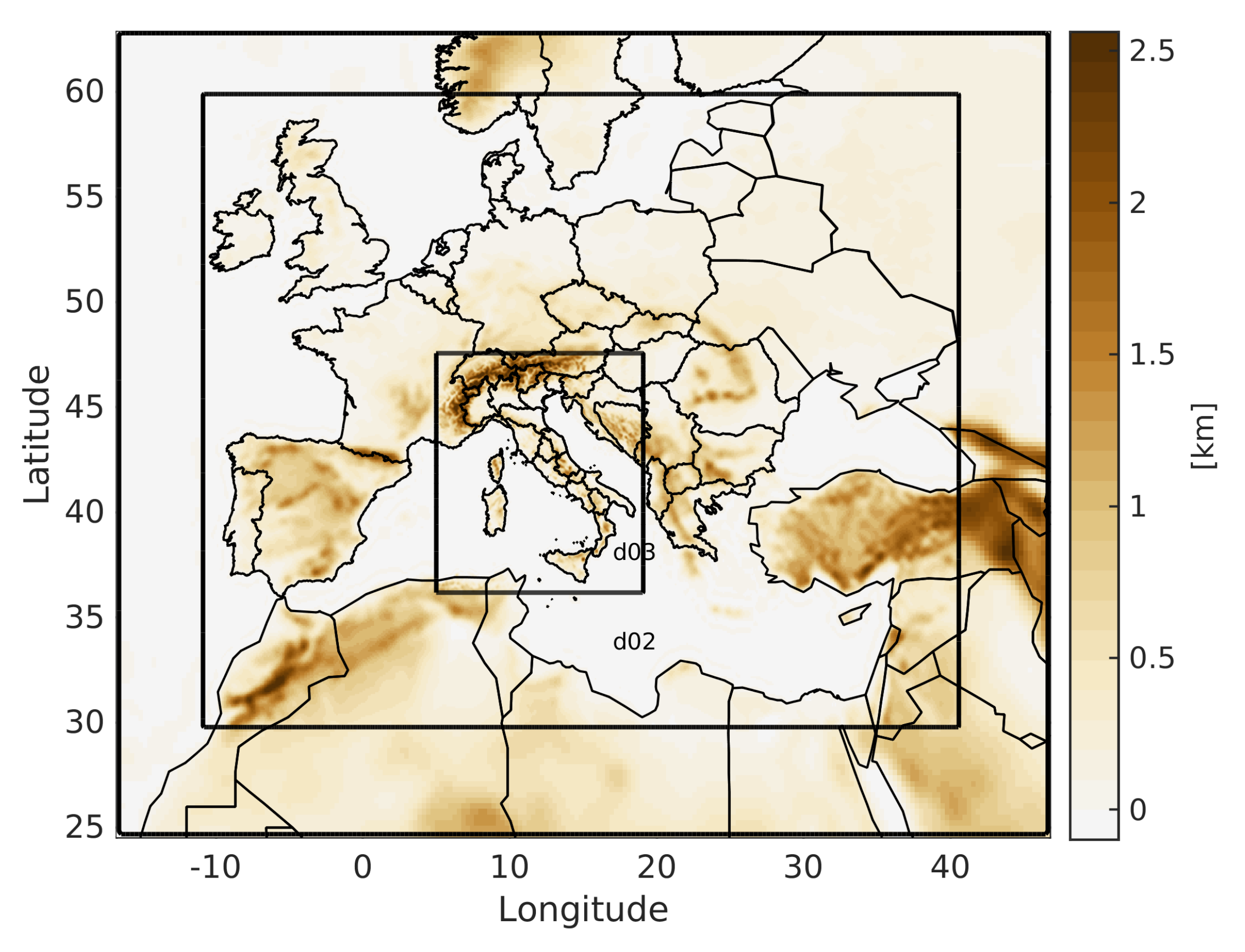
2.2. WRF Model Setup

The Weather Research and Forecasting (WRF) model v3.8.1 [34] was selected as the numerical weather model. It is a compressible non-hydrostatic model with mass-based terrain-following coordinates that was developed at the National Center for Atmospheric Research (NCAR) in collaboration with several institutes and universities for operational weather forecasting and atmospheric science research. For this study, three two-way nested domains (Figure 1) have been used. The domains have, respectively, a horizontal grid spacing of 22.5 (216 × 191 grid points), 7.5 (523 × 448) and 2.5 km (430 × 469) with 50 vertical levels (Figure 1; all domains top reach 50 hPa).

All the simulations are performed with the same physical parameterizations set, described hereafter, that has already been successfully tested in the study of similar events [7,8,30]. The MM5 scheme is adopted as surface layer [35,36,37]. A convective velocity following [38] is used to enhance surface fluxes of heat and moisture. The Rapid Update Cycle (RUC) scheme is used as a multi-level soil model (6 levels) with higher resolution in the upper soil layers (0, 5, 20, 40, 160, 300 cm). This soil model solves the heat diffusion and Richards moisture transfer equations (with a layer approach) and in the cold season considers phase changes of soil water [39,40]. The planetary boundary layer (PBL) dynamics is parameterized with the diagnostic non-local Yonsei University PBL scheme [41]. The WSM6 microphysics six-class scheme is adopted [42]. Lastly, the radiative processes are parameterized by means of the longwave and shortwave RRTMG schemes [43].

The initial and lateral boundary conditions are derived from NCEP-GFS (National Centers for Environmental Prediction Global Forecast System) analysis and forecast data available at a horizontal grid spacing of 0.25° × 0.25° and a time resolution of 3 h.

The nowcasting has been implemented with a 3-hour cycle 3DVAR technique of radar reflectivity data. The WRF data assimilation package WRFDA v3.9.1 is used. For the applied 3DVAR [8], the reflectivity operator used is the modified direct operator. This work adopts the Control Variable option 5 (CV5) of the WRFDA package for the B matrix calculation using the National Meteorological Center (NMC) method [44] (for more details, refer to WRFDA User Guide). The NMC method was applied over the entire October 2015 month with a 24 h lead time for the forecasts starting at 00:00 UTC and a 12 h lead time for the ones initialized at 12:00 UTC of the same day. The differences between the two forecasts (t + 24 and t + 12) valid for the same reference time were used to calculate the domain’s specific error statistics.

2.3. Phast Model Setup

In this work, the NWP nowcasting is improved with a radar-based probabilistic technique, PhaSt [19]. PhaSt is a spectral-based nowcasting procedure based on the precipitation fields’ empirical nonlinear transformation provided by radar measurements and on the stochastic evolution of the transformed fields in spectral space. This procedure can provide an ensemble probabilistic nowcasting of precipitation fields up to a lead time of two hours. In addition, the use of spectral space instead of physical space assures that the spatial correlations of precipitation fields are preserved. The model requires two initial precipitation fields, which are to be used as initial conditions. It takes an empirical nonlinear transformation of the two rainfall fields used as initial conditions, r(x,y,t = 0) and r(x,y,t = −Δt), and generates two Gaussian fields, g(x,y,0) and g(x,y,−Δt). The Fourier transform of the Gaussianized fields are taken, and their Fourier spectra, ĝ(kx,ky,0) and ĝ(kx,ky,−Δt) are obtained. From these, for each wavenumber (kx,ky), the Fourier phase, $\Phi$, and an estimate of the Fourier angular frequency are calculated. Fourier phases are then evolved in time by a stochastic process, while Fourier amplitudes are kept fixed. There are several stochastic models that can be used to evolve the Fourier phases. To allow the presence of time correlations in the angular frequencies, a Langevin-type model is used: the temporal evolution of the Fourier phase $\Phi$(kx,ky) at a given wavenumber (kx,ky) is written in terms of a linear Ornstein–Uhlenbeck stochastic process for the angular frequency. The Ornstein–Uhlenbeck process generates angular frequencies that have a Gaussian distribution with zero mean and variance ${\sigma }^2$ and an exponentially decaying temporal auto-correlation. The spectrum with the evolved Fourier phases is inverted to generate a nowcasted Gaussian field at the time t of interest, g(x,y,t). This evolved field has the same power spectrum as the initial Gaussianized field, g(x,y,0). Different realizations of the stochastic process allow the generation of different evolution of the precipitation field and the creation of an ensemble of precipitation nowcasts. Eventually, an inverse nonlinear transformation is performed to pass from the evolved Gaussian field g(x,y,t) to the nowcasted rainfall field.

As mentioned before, the algorithm can provide an ensemble of possible rainfall fields for the upcoming hours; in this study, however, the algorithm has been used in its deterministic version, switching off the noise related component.

2.4. Observational Dataset

The observational data used for the assimilation with the 3DVAR in WRF is the reflectivity from weather radars. These data are provided by the Meteorological Radar national mosaic operated by the Italian Civil Protection [45], CAPPI data on three levels (2000, 3000 and 5000 m a.s.l.) covering the whole Italian territory. The reflectivity data are assimilated with the modified reflectivity operator presented in [8].

The Phast algorithm uses Surface Rainfall Intensity adjusted (SRIadj) observations to nowcast the precipitation evolution. The rainfall intensity product named SRIadjust is provided by the Italian Civil Protection National Department. It is based on the National Radar Network data, which are made by different systems: C and X band radar, polarimetric and non-polarimetric radar. The algorithm to retrieve the radar quantitative precipitation estimation (RQPE) uses both polarimetric and non-polarimetric data; it is described in [46] and exploits other previous works [47,48]. The final product is obtained after adjusting RQPE with rain gauge data in a near real-time framework. Rain gauge data are interpolated with a geostatistical method described in [49] and compared with RQPE on two different accumulation time windows: 3 and 24 h.

For a certain instant t and for each pixel of the matrix grid, two Adjustment Factors are estimated as $AF=R/G$, where R is radar rain while G is gauge rain.

The $AF$ is calculated for the 24 h accumulation (AF24H) when $G>5$ mm, if $G<5$ mm $AF24H$ is not modified with respect to the previous estimation.

The $AF$ is calculated for the 3 h accumulation ($AF3H$) when $G>2$ mm, if $G<2$ mm is $AF3H$ is posed equal to $AF24H$.

The final rain field is defined as $SRIadjust=RQPE\times AF3H$; it has a spatial resolution of 1 km and a time resolution of 5 min.

Eventually, the simulation weights are calculated using the merging products between RQPE and rain gauges observations cumulated over 3 h [49,50,51].

2.5. Swing Algorithm Methodology

To deal with the main open issues related to the use of NWP models for the nowcasting applications highlighted in the Introduction, in this work, a new post-processing algorithm, SWING, is built up.

The nowcasting procedure’s aim is to produce short-term forecasts, frequently updated with observations, to provide the most reliable information on the atmospheric state in the following few hours. This would allow, with the modern communication technologies, to inform some hours in advance the population about the risks that potentially will affect a certain area.

It is well known that in order to reach this goal, NWP models at km-scale resolution need significant computational time and resources to produce on-time forecasts over large geographical areas (e.g., see the innermost domain in Figure 1). Thus, to properly design and test the nowcasting simulations for an operational purpose, it is important to consider the available HPC architecture and the time needed to run each forecast.

Along these lines, a nowcasting scheme with a 3 h cycling 3DVAR and 12 h forecast implemented to always use the most recent GFS global model available to force the NWP runs with at least two assimilation cycles before the 12 h forecast has been implemented. Figure 2 represents the nowcasting timing and forecast availability with the considered model domains setup and HPC architecture available.

The main aim is to take into account the spatial and temporal uncertainties of the meteorological model, including the consideration that the most recent simulation is not necessarily the best one due to, for example, the spin-up process. To deal with all these issues, it is important to refer to the availability time of each forecast reported in Figure 2. From that scheme, it is possible to see that, in an operational-like mode, for each time instant (dt = 3 h in this case) starting from a given time (hereafter called “now”), the nowcasting design presented this section allows to have three simulations providing a 6 h forecast (or two simulations providing a 9 h forecast) covering the same time window (Figure 3). Furthermore, each forecast has at least 3 h of simulation “in the past” with respect to the “now” instant (notice that the most recent simulation is weighted on the 3 h of forecast before the last data assimilation cycle).

The new algorithm aims to consider not only the most recent simulation at each time but all the simulations covering a given time instant and 6 h in the future. It is important to notice that every 3 h, a new forecast is available, so the nowcasting forecast will be updated every three hours starting from the “now” until the end of the use-case period.

The first time instants covered by three simulations in the chosen periods are 14 October 2019 at 06 UTC for October simulations and 12 November 2019 for the November period. Using three forecasts for each time instant has the main advantage of having different warm start times and different assimilation cycles for each of them. Each simulation is weighted based on the 3 h of forecast “in the past” with respect to the “now”. This weighting is performed through an object comparison between the simulated and observed rainfall fields (observations are from the radar and rain gauges merged maps).

When a weight for each of the three forecasts is obtained, a probability rainfall map for the following 6 h from “now” can be retrieved.

Algorithm Steps Description

The procedure described above is implemented as follows:

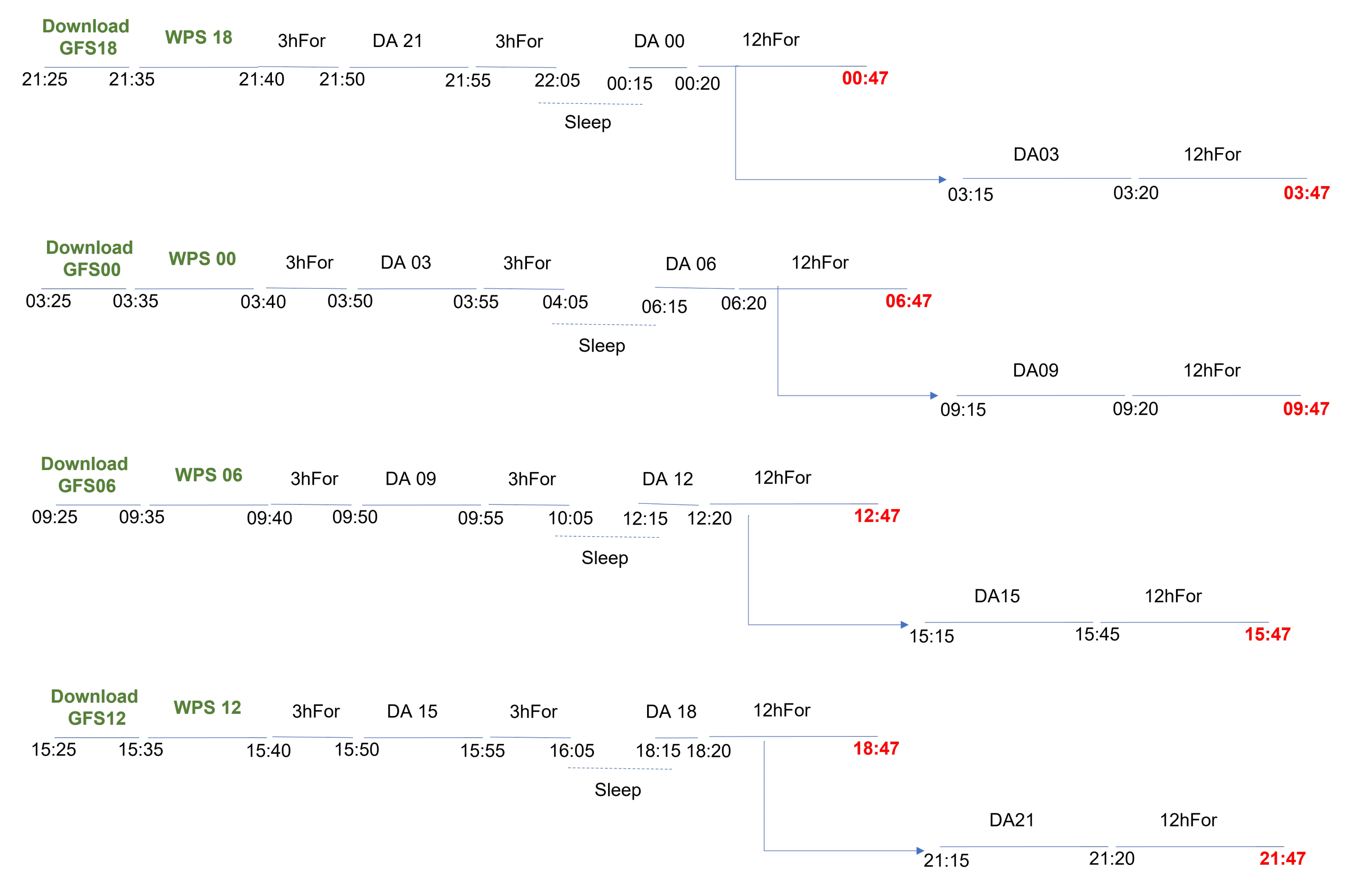
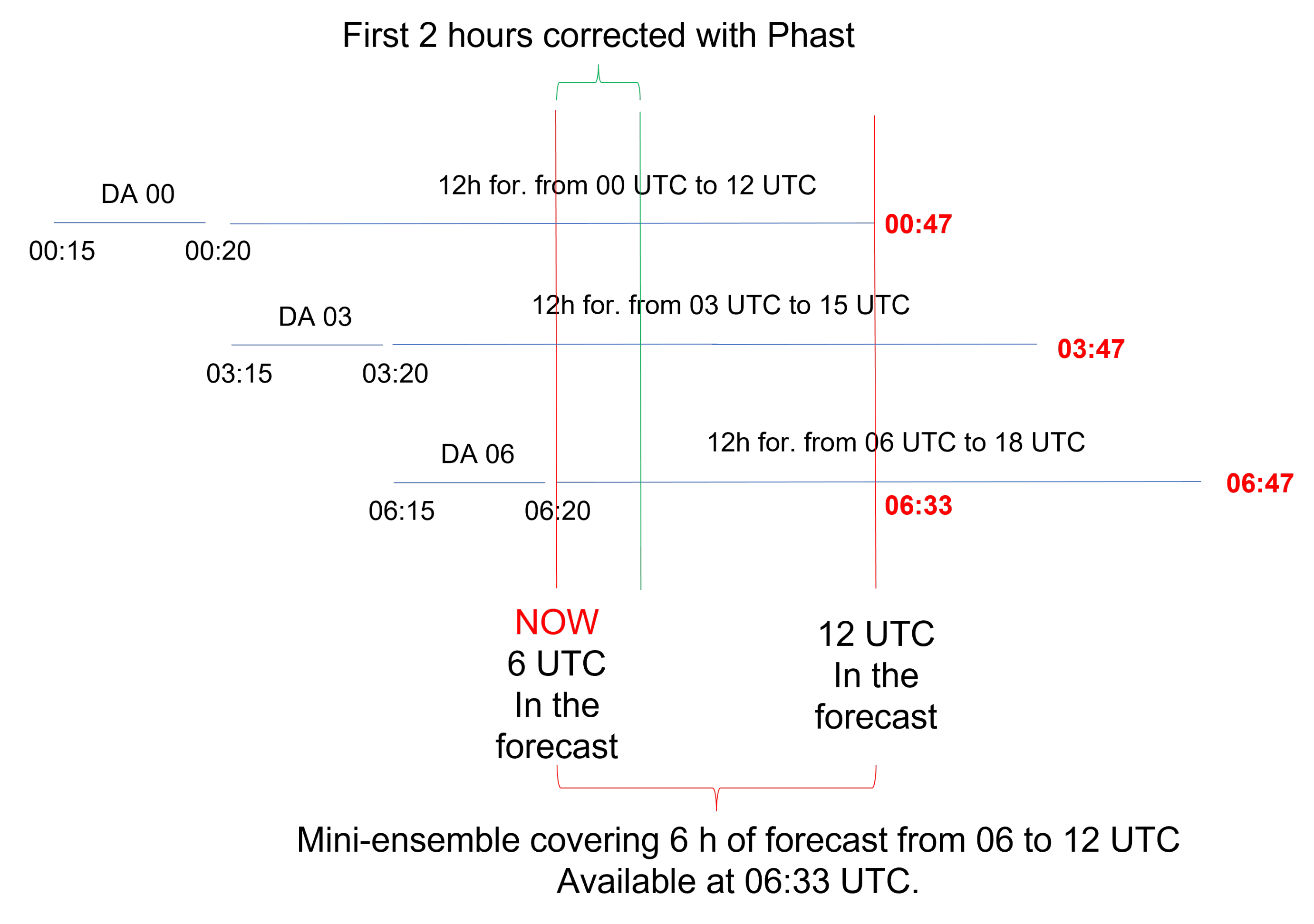
• Simulations selection: For each time instant (named hereafter “now”), there should be at least 3 h of simulation in the past used to evaluate the simulation behavior and assign a weight; then, the 6 h of future forecasts will be used to generate the rainfall probability maps.
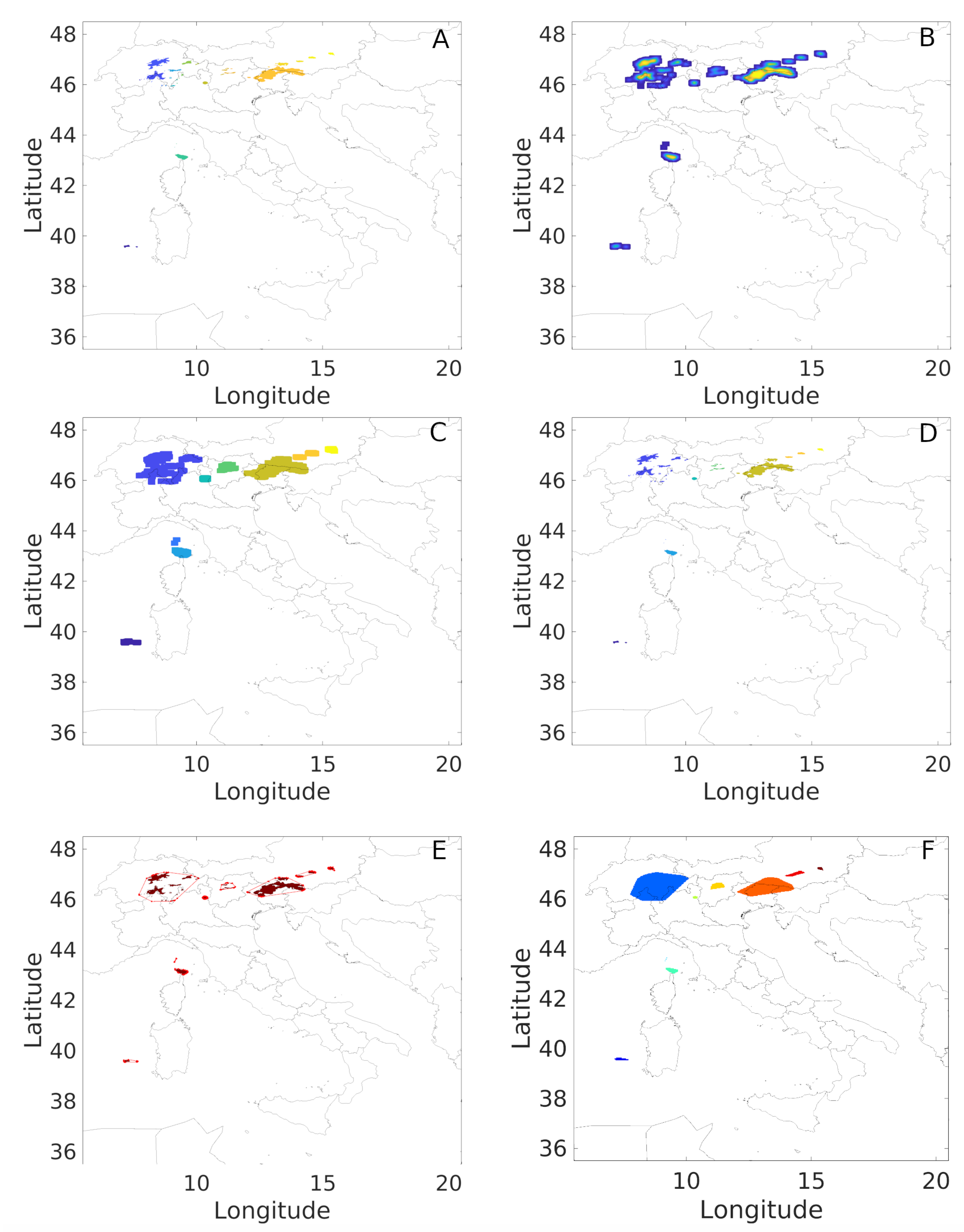
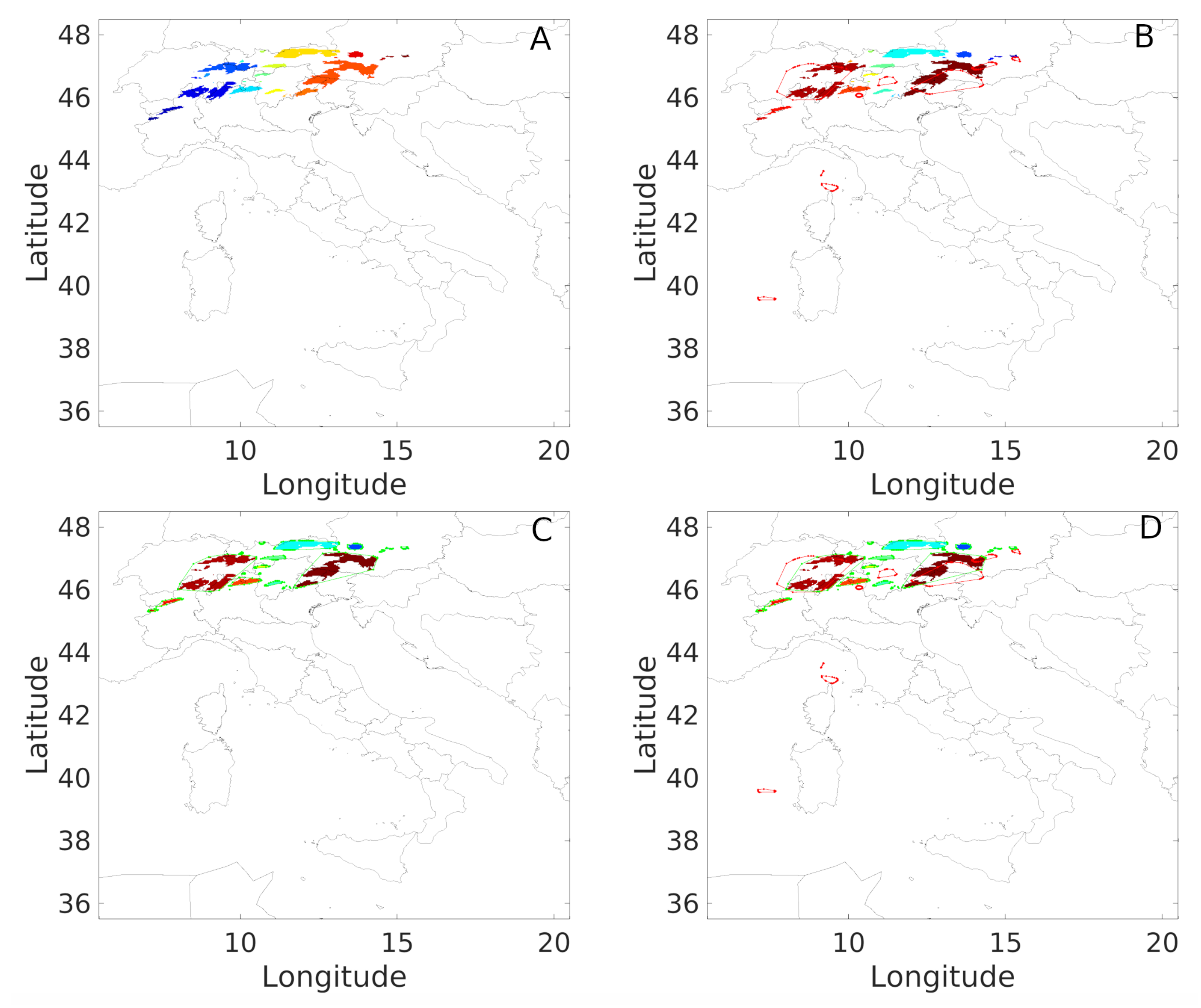
• Simulations weighting: First of all, given the observed 3 h accumulated rainfall field $P_o$, the observed rainfall objects $O_i$ are isolated considering only the regions where $P_o$ > $P_{threshold}$ (in this case, $P_{threshold}$ = 2 mm, Figure 4 panel A), obtaining the field $P_o^{\prime }$. An object $O_{Oi}$, thus, is defined as a connected region (in the sense of spatially adjacent cells) of the $P_o^{\prime }$ field in which values are different from 0. Then, a Gaussian filter GF with $\sigma$ equal to five grid points (to take into account a possible model spatial uncertainty) is applied to the observed objects to merge together those belonging to the same rainfall structure (Figure 4 panels B,C, Equation (1)).

  $$P_{oG}=GF(P_o^{\prime },5\sigma )$$

  (1)
  Then, the original data are restored into the identified objects (rainfall field $P_o$), and the convex hull of each object is calculated (Figure 4 panels D,E). Eventually, the observed objects convex hulls map $P_{CH}^O$ is produced to be used as a benchmark for modeled objects. The modeled objects $O_{Mj}$ are isolated in the same way used for the observed ones (Figure 5 panel A). In the modeled field $P_M$, instead of using a Gaussian filter to merge contiguous objects, the observed convex hulls $P_{CH}^O$ are used to merge together the modeled objects $O_{Mj}$ inside the same structure (Figure 5 panels B–D). The correspondence between the observed and the modeled objects (i is the index of observed objects, while j is the index of modeled objects) is made through the various objects characteristics scores and comparison calculation that follows:

  —

  The rainfall volumes $V_i$, $Vj$;

  —

  The areas $A_i$, $A_j$;

  —

  The distance between the centers of gravity $D_{CG}$($O_{Oi}$, $O_{Mj}$);

  —

  The objects orientation ${\alpha }_i$, ${\alpha }_j$;

  —

  The objects intersection $IA$($O_{Oi}$, $O_M$).

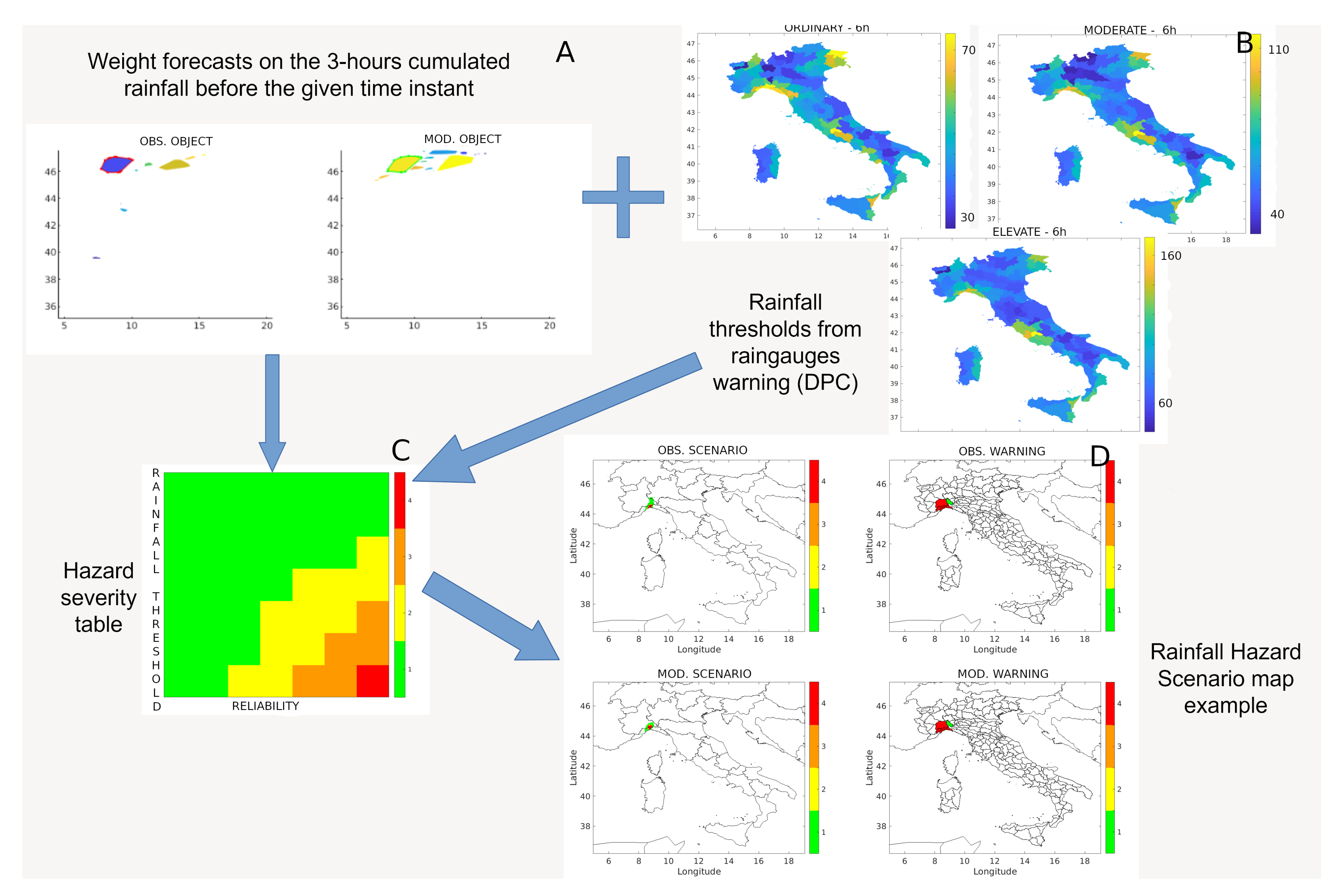
  All possible objects couples (i,j, i = 1,...,$N_O$, j = 1,...,$N_M$, with $N_O$ number of observed objects $O_{Oi}$ and $N_M$ number of modeled objects $O_M$) are tested, and all these parameters are weighted and calculated among given thresholds, allowing to obtain a proper match of observed and modeled objects. Figure 6 in panel A shows an example of objects matching. Thus, the scores above introduced are also combined in an Overall Field Score (OFS) in order to weight each simulation (Equation (2)).

  $$OFS=\frac{S_{CG}\times W_{CG}+S_A\times W_A+S_V\times W_V+S_{IA}\times W_{IA}+S_{\alpha }\times W_{\alpha }}{W_{CG}+W_A+W_V+W_{IA}+W_{\alpha }}$$

  (2)

  where $S_{CG}$ is the score distance between the center of gravity, and its weight is $W_{CG}$ = 1, $S_A$ is the area ratio score whose weight is $W_A$ = 0.25, $S_V$ is the rainfall volume score and its weight is $W_V$ = 0.5, $S_{IA}$ is the polygon intersection score, and its weight is $W_{IA}$ = 1, and eventually, $S_{\alpha }$ is the object orientation score and its weight is $W_{\alpha }$ = 0.5.
  In the final forecast weight, the OFS is combined with a missed object score MOS (observed objects not present in the model, range 0–1):

  $$MOS=1-\sum _{n=1}^{i_{matched}}{A}_i/\sum _{n=1}^{N_O}{A}_i$$

  (3)

  and a false alarm score FAS (modeled objects not present in the observation, range 0–1):

  $$FAS=exp(0.1\times \sum _{n=1}^{i_{NOTmatched}}{A}_i/\sum _{n=1}^{i_{matched}}{A}_i)$$

  (4)

  into an overall Reliability Score (RS):

  $$RS=OFS\times MOS\times FAS.$$

  (5)
  This final score is eventually used to weight the forecast for the hazard scenario production.
• Rainfall hazard scenarios production: The previously described procedure assigns the Reliability Score (RS) to each map that will be used to weight the different forecasts.
  Before the scenario generation, the first 2 h of the 6 h forecast are corrected using the Phast radar nowcasting and blended with the NWP prediction presented in Section 2.3 (Figure 3). Then, the accumulated rainfall field over the 6 h is calculated from the blended Phast and WRF model output. For each forecast, the rainfall depth in each cell is then classified according to a scale of four severity classes derived from three rainfall thresholds taken from the Italian Civil Department rain gauges warning system (Figure 6, panel B). Each precipitation severity map ($P{S}_k$) is then multiplied by its corresponding reliability score ($R{S}_k$) above introduced: in this way, a unique spatially distributed variable is obtained describing both forecast intensity and its reliability combination. Given the three forecast maps available at a certain “now” timing, the final product is the simple average of all the maps: for each pixel, thus, it represents a level of forecast hazard that synthesizes all the available forecasts weighted with their reliability (in terms, as previously described, of their ability in correctly reconstructing the previous 3 h):

  $$HS=\sum _{k=1}^{N_k}P{S}_k\times R{S}_k/N_k$$

  (6)
  We describe this as a “rainfall hazard scenario forecast”, HS, being referred to a specific forecast time window (Figure 6, Panel D-second row, left panel). To compare the forecast field with the observed one, the same procedure is applied to the radar and rain gauges merging maps considering that they have 100% occurrence probability ($R{S}_O$ = 1, Figure 6, Panel D-first row, left panel). In this map, low values can correspond to both a combination of low-intensity forecast with medium-high reliability or high-intensity forecast with low reliability: this map was conceived to yield a synthetic representation of all the information delivered by the forecast and the available observations at the map production time. In order to classify these map values, a matrix of hazard scenario intensities is provided in Figure 6, panel C, in which both rainfall forecast severity and reliability axis are represented.
• Automatic warning system: The Italian Civil Protection Department manages the hydro-meteorological warning in terms of alert areas. The Italian territory is subdivided into 170 alert areas (Figure 6, panel D, second column). Currently, the Italian Civil Protection and regional civil protection departments alert system is based on a daily bulletin issued each day before 13 UTC reporting the forecasted situation for the following 36 h for each alert area of each Italian region. In this system, a forecaster interprets the models outputs and converts them in a warning bulletin depending also on its experience (the so-called expert forecast). This approach is compatible with a common forecast delivery timing (24–48 h), while the nowcasting procedures have necessarily very frequent output (every 3 h for the SWING algorithm) with shorter forecasts (6 h in this work). Thus, the scenarios obtained with the SWING algorithm are converted automatically into warnings on the alert areas using a procedure that retrieves the warning color considering the colored pixels inside each area trying to overcome the human interpretation (Figure 6, panel D, second column).

2.6. Verification Method

As mentioned before, the modeled scenarios are automatically converted into warnings over the alert areas. Then, the same procedure is applied to the observed scenario, and eventually, the forecast is validated through a comparison between the warnings given by observations and forecasts. The alert areas warnings are provided in a colored-scale way (green, yellow, orange, red and white for no-rain areas). Thus, to validate the model’s performances, the alert areas colored by rainfall observations $H{S}_{O,a}$ are compared to the ones filled with the model outputs $H{S}_{M,a}$ where a that is the alert areas index. In this way, it is possible to highlights different behaviors:

• Correct negatives: No-rain both in modeled and observed scenarios: $H{S}_{M,a}$ = $H{S}_{O,a}$ = 0.
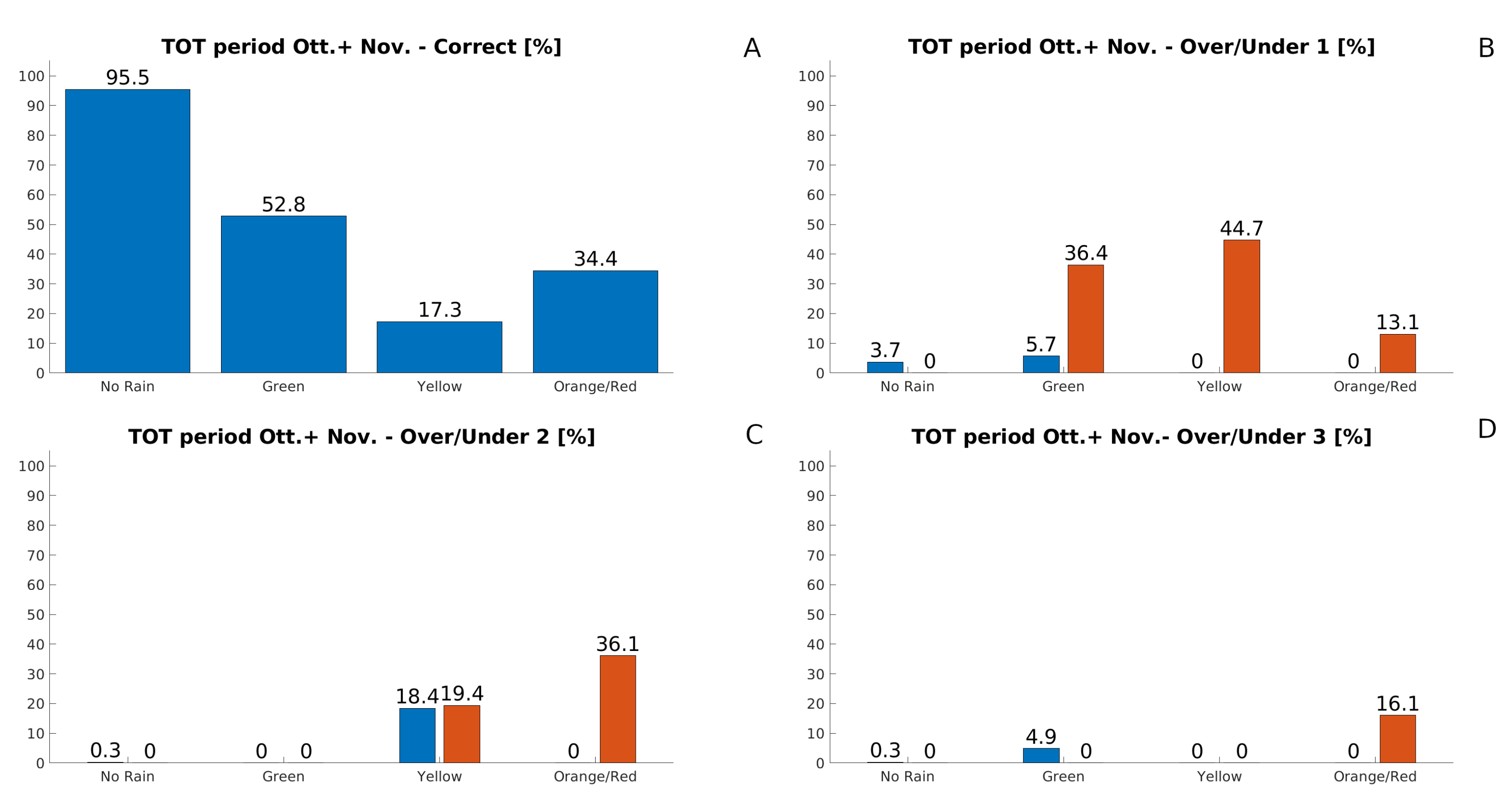
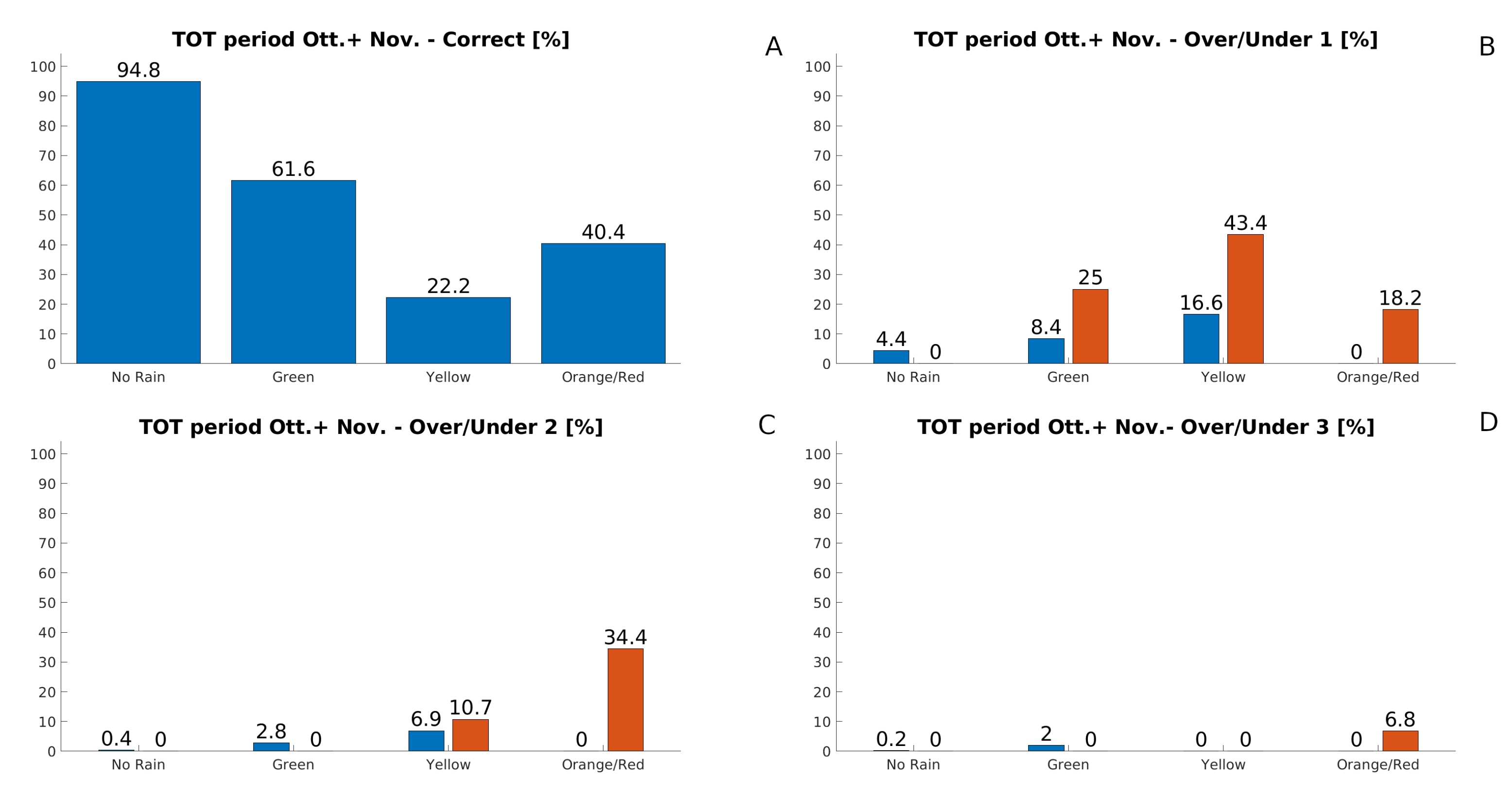
• Correct forecast: Same color both in modeled and observed scenarios: $H{S}_{M,a}$ = $H{S}_{O,a}$.
• Over/underestimation by 1: The modeled area is colored by one color more/less with respect to the observed one: $H{S}_{M,a}$−$H{S}_{O,a}$ = +/−1; i.e., the observed area is yellow and the modeled one is orange (overestimation by 1) or green (underestimation by 1).
• Over/underestimation by 2: The modeled area is colored by two colors more/less with respect to the observed one: $H{S}_{M,a}$−$H{S}_{O,a}$ = +/−2; i.e., the observed area is yellow and the modeled one is red (overestimation by 2) or white (underestimation by 2).
• Over/underestimation by 3: The modeled area is colored by three colors more/less with respect to the observed one: $H{S}_{M,a}$−$H{S}_{O,a}$ = +/−3; i.e., the observed area is green and the modeled one is red (overestimation by 3), or the observed area is red while the modeled one is green (underestimation by 3).

Over/underestimations by four colors $H{S}_{M,a}$−$H{S}_{O,a}$ = +/−4 (i.e., red observed area and white modeled area) are included into over/underestimations by three, respectively. It is worth noticing that in the Italian early warning system, the maximum alert level given for thunderstorms is orange. Thus, in an automatic procedure such as the one built in this work, orange and red alerts are counted together in the validation process, which classifies forecasts as correct when the modeled areas are orange and the corresponding observed ones are red. The validation results for each color are expressed as the percentage of the observed area of that color.

To verify the SWING algorithm performances and investigate its added value, the validation is compared with a simpler nowcasting only using only a single forecast every 3 h and with the same single forecast only corrected with the Phast nowcasting model in the first two hours.

3. Results Discussion: SWING Algorithm Application and Validation

The SWING algorithm is applied in an operational-like mode to the 22 days of October and November chosen as use cases. To evaluate the algorithm’s added value, the main idea is to compare it with the scenarios obtained with a single run forecast. The SWING algorithm is composed by two main parts; the first is the forecast correction with the Phast nowcasting tool, and the second is the small ensemble forecast weighting. Thus, the impact of each part of this system is evaluated separately. First of all, the warnings on the alert areas considering only a single simulation every 3 h (always the most recent) without Phast are evaluated (Figure 7). Secondly, to the first approach, the Phast correction is applied (Figure 8). Then, the complete SWING algorithm using Phast and the three weighted forecast is evaluated (Figure 9). Looking at Figure 7, Figure 8 and Figure 9, it is possible to see that both the use of Phast and the use of the complete SWING algorithm improves the nowcasting performance in terms of better correct forecast and less over/underestimations. More in detail, the use of Phast (comparison between Figure 7 and Figure 8) results in a higher percentage of correct forecasts (panel A of Figure 7 and Figure 8). However, the over/underestimations remain comparable with no significant changes with the exception of the underestimation of orange/red (orange bar in panel D, Figure 7 and Figure 8) that is reduced from 16.1% to 9.7%. The use of the SWING algorithm further improves some correct forecasts (green and yellow in Figure 9, panel A). Despite a slightly decrease in the correct forecast of no rain and orange/red, the main improvement obtained by the SWING algorithm relies on the strong reduction of orange/red false alarm (blue column of yellow warning in panel C Figure 7, Figure 8 and Figure 9). This means a false alarm reduction of 15.6% when the observed forecast is just a yellow warning on the alert areas while the model was forecasting an orange/red warning, overestimating the event. The reduction of such a false alarm is very important for the public’s perception of danger when an orange/red warning is issued, because false alarms may reduce confidence in future warnings, and thus, over-warning can be problematic [52,53,54]. Furthermore, a quite general improvement is obtained with the SWING algorithm for what concerns the underestimations (orange bars) with the exception of the orange/red underestimation by 1 and 2 (panels B and C) that slightly increases. However, there, the worst underestimation (by 3) is further reduced with the SWING algorithm (panels D). The main issue still remains an underestimation by 2 (orange column in panel C) of 34.4% of orange/red warnings: future works will be devoted to further improve also this aspect.

Another aspect worth evaluating is the forecast timing. In fact, the SWING algorithm must provide a correct forecast in useful timing to be issued to the population sufficiently in advance to allow some self-protective behavior. For this investigation, the analysis was centered on the two most intense events: 14/15 October 2019 and 21/22 October 2019. The first event is very localized in time and space; it is a typical organized thunderstorm [7,8,30] that has more than 400 mm of rain fall down in about 6 h in a very small area. The rainfall started between 22 and 23 UTC in the evening of 14 October (depending on the location) and continued until 06 UTC. So, we will consider the last useful forecast that can be available: the 21 UTC forecast (Figure 10). As it is possible to see from Figure 10, the modeled scenario (panel C) is very close to the observed one (panel A). Furthermore, the automatic warnings on the corresponding alert areas perfectly match (panel B observation, panel D model). Referring to the timing of Figure 2 and Figure 3, the 21 UTC forecast is available around 21:30 UTC. This means that with an automatic warning diffusion, people could be advised half an hour to one hour before the event beginning.

The second intense event timing is more complicated to evaluate: in fact, it is a longer-lasting event started on 19 October, with the most intense part during 21 October with precipitation peaking up to 400 mm in 12 h in some Piedmont area [21]. Indeed, on 21 October, a first Mesoscale Convective System (MCS) moved from Marseilles and the French coast to the Italian central Alps (Lombardy region) in about 6 h between 00 UTC and 06 UTC. After this first convective episode in the morning, a second very intense V-shape MCS took place between Liguria and Piedmont regions starting from 12 UTC and persisting over the same area for about 12 h with the most intense phase between 18 UTC and 00 UTC. The above-mentioned dynamic makes the forecast timing very difficult, because MCSs (especially V-shapes) have an intrinsic high difficult forecast capability, and the main issues during 21 October are due to two such intense events persisting over areas with already saturated soil from previous rainfall days. It is worth further noticing also that the V-shape event of 21 and 22 October was completely missed by all the operational models available for the daily forecast. To look at the first MCS passing from the French coast to the central Italian Alps in the first 6 h of 21 October, Figure 11 and Figure 12 show the 00 UTC and 03 UTC forecasts for the next 6 h. In the 00 UTC forecast, the model tends to underestimate a bit the event extension with less alert areas with orange/red color (Figure 11, panel D) with respect to the observed ones (Figure 11, panel B). At 03 UTC, instead, the modeled area with at least an orange warning (the maximum for thunderstorm in the current Italian early warning system) is better covering the red observed areas (Figure 12, panels B and D).

The V-shape MCS that hits northwestern Italy in the afternoon is even more difficult to be predicted. The beginning of this event at 12 UTC is shifted by the model to the north with respect to the observed red warning (Figure 13). However, looking at the 18 UTC forecast (Figure 14), the model is able to warn with at least an orange warning the alert areas most hit by the intense phase of this second event for the following six hours.

From the results presented, the SWING algorithm can improve the forecast capability with respect to a traditional single run nowcasting and thus integrate the current forecast procedures, allowing an automatic warning of people in case of extreme events with an overall good performance also in case of hardly predictable events. The algorithm improves the correct forecast, but above all, the results are very effective in the control of over/underestimation that could affect the forecast reliability perception by people. However, the main advantage of this algorithm is its high versatility. In fact, here, it is used with the WRF meteorological model, but it can be applied to every model output also in the multi-model approach. Furthermore, the scenarios can be calculated on a larger ensemble members number. Thus, it can pave the way for future improvements related to the use of a multi-model approach or an ensemble members increase used to build the scenarios (depending on computational resources). Eventually, depending on the application, the warning can be calculated also on different areas such as municipalities or provinces instead of the alert areas used here for conventional civil protection applications or on different variables such as the lightning potential index (LPI [30]), to predict lightning risk as an example.

4. Conclusions

In this work, starting from the actual NWP models’ capability in terms of nowcasting and the always-growing needs for accurate short-range forecasts, the new SWING algorithm is introduced. This system aims to combine the state-of-the-art nowcasting knowledge with a new post-processing algorithm (SWING) able to take the best from the combination of the Phast nowcasting model and the NWP model WRF improved with a 3 h rapid update cycling 3DVAR. This algorithm tries to take into account the timely and spatial model uncertainty in the convective field simulation and to obtain the best correct forecast as possible containing false alarms. Furthermore, it is worth noticing that in a nowcasting context, with a rapid forecast update (every 3 h in this case), there is no time for a forecast issued by an expert meteorologist. We are aware that there is still an added value in the human forecast correction [55], but in such a framework, the time might be not enough. Thus, the SWING algorithm tries to provide a direct warning on the Italian Civil Protection Alert Areas so that people could be informed of imminent dangers more rapidly.

The SWING algorithm is tested on 22 days during the fall season 2019, 14–22 October and 12–24 November. This test provided good SWING performances statistics with different rainfall regimes. Inside the 22 days, there are also two main extreme events allowing to test the performances in a very intense and localized (in time and space) event (14 and 15 October 2019) and in more extended extreme events (21 and 22 October 2019). First of all, the algorithm results are overall evaluated by comparing the SWING performances with the use of a deterministic single simulation both with and without the Phast nowcasting blended to the model. This first analysis revealed that the complete SWING algorithm use is able to provide the best correct forecast performance, maintaining overestimation and underestimation under control better than using a single deterministic forecast both with or without Phast. Moreover, the use of Phast allows to further improve the forecast skill and reduce the over/underestimation. In the second part of the discussion, another important point is analyzed: the SWING forecasts’ useful timing. For this, the focus is moved only to the two extreme events. In the 14 October event, thanks to the SWING algorithm, people can be advised half an hour to one hour before the event beginning (depending on the location). The second event (21 and 22 October 2019) was harder to predict, because it was a longer (in terms of time) event with two main MCSs persisting over the same areas with already saturated soil from previous rainfall days. In this case, the SWING algorithm was almost able to properly capture the first MCS passage from the French coast to the central Italian Alps, despite some underestimation in terms of area extension at the beginning. The second MCS was a V-shape storm, which is even more difficult to predict. In this case, the model is able to warn with at least an orange color the alert areas mostly hit by the intense phase of this second event for the following six hours. However, in this case, the V-shape beginning is shifted by the model a bit northern with respect to the observed red warning areas.

From these results, the SWING algorithm can improve the predictive capability of a traditional deterministic nowcasting forecast system, keeping a useful forecast timing and thus integrating the current forecast procedures. This allows an automatic warning of people in case of extreme events with an overall good performance also in case of hardly predictable events.

However, the main advantage of the SWING algorithm is not only in the performances here presented but also its very high versatility. It can be applied to every model output, allowing also to test a multi-model approach, and the scenarios can be calculated with more ensemble members (depending on computational resources). It can be used with different assimilation techniques and different kinds of observations. Eventually, depending on the application, the warning can be calculated also for different areas such as municipalities or provinces instead of the alert areas used here for conventional civil protection applications or on different variables such as the lightning potential index (LPI, [30]) to predict lightning risk. The results obtained in this work with the SWING algorithm pave the way for future research such as the use of a multi-model approach using both the simulations from WRF and other models (i.e., ICON Model, [56]), the use of other observations for the assimilation to further improve the forecast skill (such as lightning assimilation) or the test of an ensemble with more members trying to obtain the best cost (computational resources)–benefits (better forecast) as possible.

References

1. Sideris, I.V.; Foresti, L.; Nerini, D.; Germann, U. NowPrecip: Localized precipitation nowcasting in the complex terrain of Switzerland. Q. J. R. Meteorol. Soc. 2020, 146, 1768–1800. [Google Scholar] [CrossRef]
2. Sättele, M.; Bründl, M.; Straub, D. A classification of warning system for natural hazards. In Proceedings of the 10th International Probabilistic Workshop, Stuttgart, Germany, 15–16 November 2012; pp. 257–270. [Google Scholar]
3. Twardosz, R.; Walanus, A.; Guzik, I. Warming in Europe: Recent trends in annual and seasonal temperatures. Pure Appl. Geophys. 2021, 178, 4021–4032. [Google Scholar] [CrossRef]
4. Gaume, E.; Borga, M.; Llassat, M.C.; Maouche, S.; Lang, M.; Diakakis, M. Mediterranean extreme floods and flash floods. Mediterr. Reg. Clim. Change 2016, 133–144. [Google Scholar]
5. Rebora, N.; Molini, L.; Casella, E.; Comellas, A.; Fiori, E.; Pignone, F.; Siccardi, F.; Silvestro, F.; Tanelli, S.; Parodi, A. Extreme rainfall in the Mediterranean: What can we learn from observations? J. Hydrometeorol. 2013, 14, 906–922. [Google Scholar] [CrossRef]
6. Ducrocq, V.; Braud, I.; Davolio, S.; Ferretti, R.; Flamant, C.; Jansa, A.; Kalthoff, N.; Richard, E.; Taupier-Letage, I.; Ayral, P.A.; et al. HyMeX-SOP1: The field campaign dedicated to heavy precipitation and flash flooding in the northwestern Mediterranean. Bull. Am. Meteorol. Soc. 2014, 95, 1083–1100. [Google Scholar] [CrossRef] [Green Version]
7. Fiori, E.; Ferraris, L.; Molini, L.; Siccardi, F.; Kranzlmueller, D.; Parodi, A. Triggering and evolution of a deep convective system in the Mediterranean sea: Modelling and observations at a very fine scale. Q. J. R. Meteorol. Soc. 2017, 143, 927–941. [Google Scholar] [CrossRef]
8. Lagasio, M.; Silvestro, F.; Campo, L.; Parodi, A. Predictive capability of a high-resolution hydrometeorological forecasting framework coupling WRF cycling 3dvar and Continuum. J. Hydrol. 2019, 20, 1307–1337. [Google Scholar] [CrossRef]
9. Done, J.; Davis, C.A.; Weisman, M. The next generation of NWP: Explicit forecasts of convection using the Weather Research and Forecasting (WRF) model. Atmos. Sci. Lett. 2004, 5, 110–117. [Google Scholar] [CrossRef]
10. Kain, J.S.; Weiss, S.J.; Levit, J.J.; Baldwin, M.E.; Bright, D.R. Examination of convection-allowing configurations of the WRF model for the prediction of severe convective weather: The SPC/NSSL Spring Program 2004. Weather Forecast. 2006, 21, 167–181. [Google Scholar] [CrossRef] [Green Version]
11. Weisman, M.L.; Davis, C.; Wang, W.; Manning, K.W.; Klemp, J.B. Experiences with 0–36-h explicit convective forecasts with the WRF-ARW model. Weather Forecast. 2008, 23, 407–437. [Google Scholar] [CrossRef]
12. Clark, A.J.; Gallus, W.A., Jr.; Xue, M.; Kong, F. A comparison of precipitation forecast skill between small convection-allowing and large convection-parameterizing ensembles. Weather Forecast. 2009, 24, 1121–1140. [Google Scholar] [CrossRef] [Green Version]
13. Sun, J.; Xue, M.; Wilson, J.W.; Zawadzki, I.; Ballard, S.P.; Onvlee-Hooimeyer, J.; Joe, P.; Barker, D.M.; Li, P.W.; Golding, B.; et al. Use of NWP for nowcasting convective precipitation: Recent progress and challenges. Bull. Am. Meteorol. Soc. 2014, 95, 409–426. [Google Scholar] [CrossRef] [Green Version]
14. Benjamin, S.G.; Dévényi, D.; Weygandt, S.S.; Brundage, K.J.; Brown, J.M.; Grell, G.A.; Kim, D.; Schwartz, B.E.; Smirnova, T.G.; Smith, T.L.; et al. An hourly assimilation–forecast cycle: The RUC. Mon. Weather Rev. 2004, 132, 495–518. [Google Scholar] [CrossRef]
15. Sun, J.; Trier, S.B.; Xiao, Q.; Weisman, M.L.; Wang, H.; Ying, Z.; Xu, M.; Zhang, Y. Sensitivity of 0–12-h warm-season precipitation forecasts over the central United States to model initialization. Weather Forecast. 2012, 27, 832–855. [Google Scholar] [CrossRef]
16. Germann, U.; Zawadzki, I.; Turner, B. Predictability of precipitation from continental radar images. Part IV: Limits to prediction. J. Atmos. Sci. 2006, 63, 2092–2108. [Google Scholar] [CrossRef]
17. Golding, B. Nimrod: A system for generating automated very short range forecasts. Meteor. Appl. 1998, 5, 1–16. [Google Scholar] [CrossRef]
18. Poletti, M.L.; Silvestro, F.; Davolio, S.; Pignone, F.; Rebora, N. Using nowcasting technique and data assimilation in a meteorological model to improve very short range hydrological forecasts. Hydrol. Earth Syst. Sci. 2019, 23, 3823–3841. [Google Scholar] [CrossRef] [Green Version]
19. Metta, S.; von Hardenberg, J.; Ferraris, L.; Rebora, N.; Provenzale, A. Precipitation nowcasting by a spectral-based nonlinear stochastic model. J. Hydrometeorol. 2009, 10, 1285–1297. [Google Scholar] [CrossRef]
20. Arpa Liguria. Report 173-14-20 Ottobre 2019. 2019. Available online: https://www.arpal.liguria.it/contenuti_statici/pubblicazioni/rapporti_eventi/2019/Report_speditivo_20191014-20191108_vers20191118.pdf (accessed on 30 May 2022). (In Italian).
21. Arpa Piemonte. Eventi Idrometeorologici Dal 19 al 24 Ottobre 2019. 2019. Available online: http://www.arpa.piemonte.it/news/pubblicato-il-rapporto-sugli-eventi-idrometeorologici-di-ottobre-2019 (accessed on 30 May 2022). (In Italian).
22. Molini, L.; Parodi, A.; Rebora, N.; Craig, G.C. Classifying severe rainfall events over Italy by hydrometeorological and dynamical criteria. Q. J. R. Meteorol. Soc. 2011, 137, 148–154. [Google Scholar] [CrossRef]
23. Lagasio, M.; Meroni, A.N.; Boni, G.; Pulvirenti, L.; Monti-Guarnieri, A.; Haagmans, R.; Hobbs, S.; Parodi, A. Meteorological osses for new zenith total delay observations: Impact assessment for the hydroterra geosynchronous satellite on the october 2019 genoa event. Remote Sens. 2020, 12, 3787. [Google Scholar] [CrossRef]
24. Parodi, A.; Boni, G.; Ferraris, L.; Siccardi, F.; Pagliara, P.; Trovatore, E.; Foufoula-Georgiou, E.; Kranzlmueller, D. The “perfect storm”: From across the Atlantic to the hills of Genoa. Eos Trans. Am. Geophys. Union 2012, 93, 225–226. [Google Scholar] [CrossRef]
25. Fiori, E.; Comellas, A.; Molini, L.; Rebora, N.; Siccardi, F.; Gochis, D.; Tanelli, S.; Parodi, A. Analysis and hindcast simulations of an extreme rainfall event in the Mediterranean area: The Genoa 2011 case. Atmos. Res. 2014, 138, 13–29. [Google Scholar] [CrossRef] [Green Version]
26. Duffourg, F.; Nuissier, O.; Ducrocq, V.; Flamant, C.; Chazette, P.; Delanoë, J.; Doerenbecher, A.; Fourrié, N.; Di Girolamo, P.; Lac, C.; et al. Offshore deep convection initiation and maintenance during the HyMeX IOP 16a heavy precipitation event. Q. J. R. Meteorol. Soc. 2016, 142, 259–274. [Google Scholar] [CrossRef]
27. Silvestro, F.; Rebora, N.; Giannoni, F.; Cavallo, A.; Ferraris, L. The flash flood of the Bisagno Creek on 9th October 2014: An “unfortunate” combination of spatial and temporal scales. J. Hydrol. 2016, 541, 50–62. [Google Scholar] [CrossRef] [Green Version]
28. Silvestro, F.; Rebora, N.; Rossi, L.; Dolia, D.; Gabellani, S.; Pignone, F.; Trasforini, E.; Rudari, R.; De Angeli, S.; Masciulli, C. What if the 25 October 2011 event that struck Cinque Terre (Liguria) had happened in Genoa, Italy? Flooding scenarios, hazard mapping and damage estimation. Nat. Hazards Earth Syst. Sci. 2016, 16, 1737–1753. [Google Scholar] [CrossRef] [Green Version]
29. Cassola, F.; Ferrari, F.; Mazzino, A.; Miglietta, M. The role of the sea on the flash floods events over Liguria (northwestern Italy). Geophys. Res. Lett. 2016, 43, 3534–3542. [Google Scholar] [CrossRef]
30. Lagasio, M.; Parodi, A.; Procopio, R.; Rachidi, F.; Fiori, E. Lightning potential index performances in multimicrophysical cloud-resolving simulations of a back-building mesoscale convective system: The Genoa 2014 event. J. Geophys. Res. Atmos. 2017, 122, 4238–4257. [Google Scholar] [CrossRef]
31. Parodi, A.; Ferraris, L.; Gallus, W.; Maugeri, M.; Molini, L.; Siccardi, F.; Boni, G. Ensemble cloud-resolving modelling of a historic back-building mesoscale convective system over Liguria: The San Fruttuoso case of 1915. Clim. Past 2017, 13, 455–472. [Google Scholar] [CrossRef] [Green Version]
32. Faccini, F.; Piccazzo, M.; Robbiano, A. Natural hazards in San Fruttuoso of Camogli (Portofino Park, Italy): A case study of a debris flow in a coastal environment. Boll. Della Soc. Geol. Ital. 2009, 128, 641–654. [Google Scholar]
33. Maifredi, P. Ancient big landslide evolution and related effects on floods in Genoa in 1953, 1970 and. Nat. Risk Civ. Prot. 1995, 16050, 237. [Google Scholar]
34. Skamarock, W.C.; Klemp, J.B.; Dudhia, J.; Gill, D.O.; Barker, D.M.; Duda, M.; Wang, X.Y.; Wang, W.; Power, J.G. A Description of the Advanced Research WRF Version 3. In NCAR Technical Note-475+ STR; National Center for Atmospheric Research: Boulder, CO, USA, 2008; p. 113. [Google Scholar] [CrossRef]
35. Paulson, C.A. The mathematical representation of wind speed and temperature profiles in the unstable atmospheric surface layer. J. Appl. Meteorol. 1970, 9, 857–860. [Google Scholar] [CrossRef]
36. Dyer, A.J.; Hicks, B.B. Flux-gradient relationships in the constant flux layer. Q. J. R. Meteorol. Soc. 1970, 96, 715–721. [Google Scholar] [CrossRef]
37. Webb, E.K. Profile relationships: The log-linear range, and extension to strong stability. Q. J. R. Meteorol. Soc. 1970, 96, 67–90. [Google Scholar] [CrossRef]
38. Beljaars, A.C. The parametrization of surface fluxes in large-scale models under free convection. Q. J. R. Meteorol. Soc. 1995, 121, 255–270. [Google Scholar] [CrossRef]
39. Smirnova, T.G.; Brown, J.M.; Benjamin, S.G. Performance of different soil model configurations in simulating ground surface temperature and surface fluxes. Mon. Weather Rev. 1997, 125, 1870–1884. [Google Scholar] [CrossRef]
40. Smirnova, T.G.; Brown, J.M.; Benjamin, S.G.; Kim, D. Parameterization of cold season processes in the MAPS land-surface scheme. J. Geophys. Res. 2000, 105, 4077–4086. [Google Scholar] [CrossRef]
41. Hong, S.Y.; Noh, Y.; Dudhia, J. A new vertical diffusion package with an explicit treatment of entrainment processes. Mon. Weather Rev. 2006, 134, 2318–2341. [Google Scholar] [CrossRef] [Green Version]
42. Hong, S.Y.; Lim, J.O.J. The WRF single-moment 6-class microphysics scheme (WSM6). J. Korean Meteorol. Soc. 2006, 42, 129–151. [Google Scholar]
43. Iacono, M.J.; Delamere, J.S.; Mlawer, E.J.; Shephard, M.W.; Clough, S.A.; Collins, W.D. Radiative forcing by long-lived greenhouse gases: Calculations with the AER radiative transfer models. J. Geophys. Res. Atmos. 2008, 113, D13103. [Google Scholar] [CrossRef]
44. Wang, H.; Huang, X.Y.; Sun, J.; Xu, D.; Zhang, M.; Fan, S.; Zhong, J. Inhomogeneous background error modeling for WRF-Var using the NMC method. J. Appl. Meteor. Climatol. 2014, 53, 2287–2309. [Google Scholar] [CrossRef] [Green Version]
45. Vulpiani, G.; Pagliara, P.; Negri, M.; Rossi, L.; Gioia, A.; Giordano, P.; Alberoni, P.P.; Cremonini, R.; Ferraris, L.; Marzano, F.S. The Italian radar network within the national early-warning system for multi-risks management. In Proceedings of the Fifth European Conference on Radar in Meteorology and Hydrology (ERAD 2008), Helsinki, Finland, 30 June–4 July 2008; Volume 184. [Google Scholar]
46. Vulpiani, G.; Guerriero, E.; Giordano, P.; Negri, M.; Pagliara, P. The Italian radar QPE: Description performance analysis and perspectives. In Proceedings of the 15th Plinius Conference on Mediterranean Risks, Giardini, Naxos, Italy, 8–11 June 2016. [Google Scholar]
47. Vulpiani, G.; Montopoli, M.; Passeri, L.D.; Gioia, A.G.; Giordano, P.; Marzano, F.S. On the use of dual-polarized C-band radar for operational rainfall retrieval in mountainous areas. J. Appl. Meteorol. Climatol. 2012, 51, 405–425. [Google Scholar] [CrossRef]
48. Vulpiani, G.; Baldini, L.; Roberto, N. Characterization of Mediterranean hail-bearing storms using an operational polarimetric X-band radar. Atmos. Meas. Technol. 2015, 8, 4681–4698. [Google Scholar] [CrossRef] [Green Version]
49. Bruno, G.; Pignone, F.; Silvestro, F.; Gabellani, S.; Schiavi, F.; Rebora, N.; Giordano, P.; Falzacappa, M. Performing Hydrological Monitoring at a National Scale by Exploiting Rain-Gauge and Radar Networks: The Italian Case. Atmosphere 2021, 12, 771. [Google Scholar] [CrossRef]
50. Sinclair, S.; Pegram, G. Combining radar and rain gauge rainfall estimates using conditional merging. Atmos. Sci. Lett. 2005, 6, 19–22. [Google Scholar] [CrossRef]
51. Pignone, F.; Rebora, N. GRISO: Rainfall Generator of Spatial Interpolation from Observation. In Proceedings of the EGU General Assembly Conference Abstracts, Vienna, Austria, 27 April–2 May 2014; Volume 16. [Google Scholar]
52. Roulston, M.S.; Smith, L.A. The boy who cried wolf revisited: The impact of false alarm intolerance on cost–loss scenarios. Weather Forecast. 2004, 19, 391–397. [Google Scholar] [CrossRef]
53. Barnes, L.R.; Gruntfest, E.C.; Hayden, M.H.; Schultz, D.M.; Benight, C. False alarms and close calls: A conceptual model of warning accuracy. Weather Forecast. 2007, 22, 1140–1147. [Google Scholar] [CrossRef]
54. LeClerc, J.; Joslyn, S. The cry wolf effect and weather-related decision making. Risk Anal. 2015, 35, 385–395. [Google Scholar] [CrossRef]
55. Turco, M.; Milelli, M. The forecaster’s added value in QPF. Adv. Geosci. 2010, 25, 29–36. [Google Scholar] [CrossRef] [Green Version]
56. Zängl, G.; Reinert, D.; Rípodas, P.; Baldauf, M. The ICON (ICOsahedral Nonhydrostatic) modelling framework of DWD and MPI-M: Description of the nonhydrostatic dynamical core. Q. J. R. Meteorol. Soc. 2015, 141, 563–579. [Google Scholar] [CrossRef]
Figure 1. The three nested domains adopted for the WRF model.
Water 14 02131 g001
Figure 2. Nowcasting scheme with the operational timing obtained with the available HPC architecture.
Water 14 02131 g002
Figure 3. Ensemble example from timing reported in Figure 2.
Water 14 02131 g003
Figure 4. SWING procedure on observed objects: Panel (A) observed objects, Panel (B) Gaussian filter with sigma = 5, Panel (C) Merged observed object, Panel (D) observed object grouped together, Panel (E) convex hulls around grouped objects, Panel (F) map of merged object.
Water 14 02131 g004
Figure 5. SWING procedure on modeled objects: Panel (A) modeled objects, Panel (B) grouped modeled object over observed convex hulls, Panel (C) modeled convex hulls, Panel (D) observed and modeled convex hulls comparison.
Water 14 02131 g005
Figure 6. SWING hazard scenarios generation. Starting from the forecasts weightings with respect to observations (Panel (A)) and the rainfall thresholds from the Italian Civil Protection Department warning system (Panel (B)), the hazard level for each rainfall object is retrieved from the hazard severity table (Panel (C)). Eventually, the hazard scenario maps and the warning on the alert areas are obtained (Panel (D)).
Water 14 02131 g006
Figure 7. Performance obtained using only a single run. In panels (BD), overestimations are represented in blue and underestimations are in orange, panel (A) represents the correct forecast percentage.
Water 14 02131 g007
Figure 8. Performance obtained using only a single run corrected with Phast. In panels (BD), overestimations are represented in blue and underestimations are represented in orange, panel (A) represents the correct forecast percentage.
Water 14 02131 g008
Figure 9. Performance obtained using the complete SWING algorithm. In panels (BD), overestimations are represented in blue and underestimations are represented in orange, panel (A) represents the correct forecast percentage.
Water 14 02131 g009
Figure 10. Scenario generated for the 14 October 2019 event at 21 UTC. Panels (A,B) refer to observed scenario, panels (C,D) to the modeled one.
Water 14 02131 g010
Figure 11. Scenario generated for the 21 October 2019 event at 00 UTC for the next 6 h. Panels (A,B) refer to observed scenario, panels (C,D) to the modeled one.
Water 14 02131 g011
Figure 12. Scenario generated for the 21 October 2019 event at 03 UTC for the next 6 h. Panels (A,B) refer to observed scenario, panels (C,D) to the modeled one.
Water 14 02131 g012
Figure 13. Scenario generated for the 21 October 2019 event at 12 UTC for the next 6 h. Panels (A,B) refer to observed scenario, panels (C,D) to the modeled one.
Water 14 02131 g013
Figure 14. Scenario generated for the 21 October 2019 event at 18 UTC for the next 6 h. Panels (A,B) refer to observed scenario, panels (C,D) to the modeled one.
Water 14 02131 g014
Publisher’s Note: MDPI stays neutral with regard to jurisdictional claims in published maps and institutional affiliations.