
Generating Continuous Rainfall Time Series with High Temporal Resolution by Using a Stochastic Rainfall Generator with a Copula and Modified Huff Rainfall Curves


Abstract
:1. Introduction
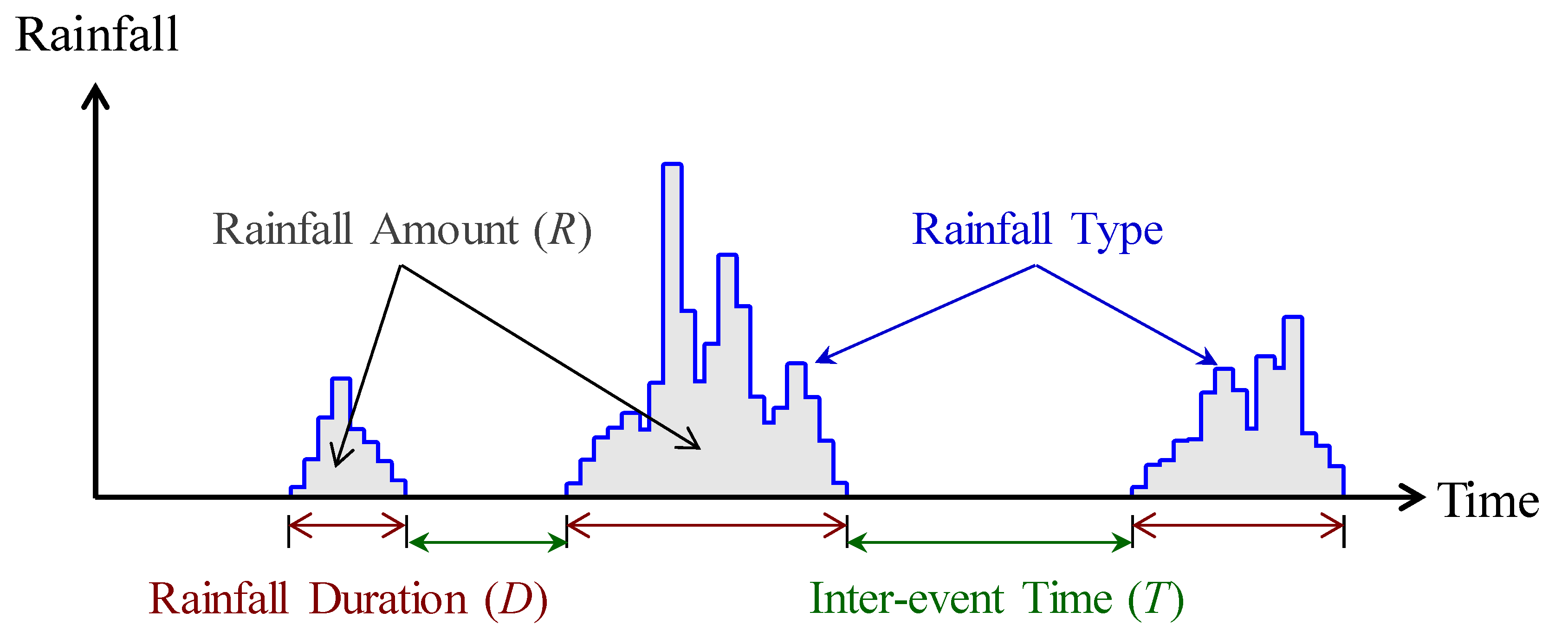
2. Methodology
2.1. Continuous Rainfall Time Series Generation
2.2. Bivariate Copula
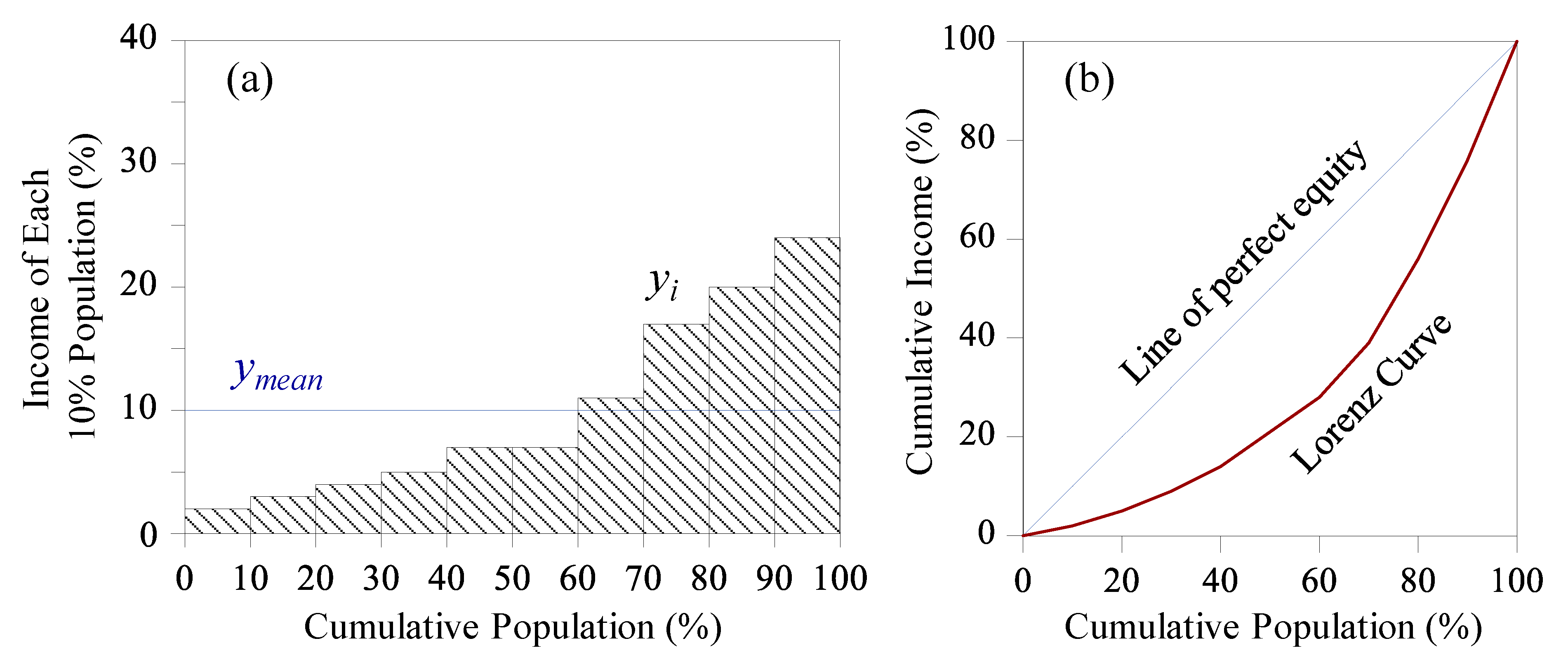
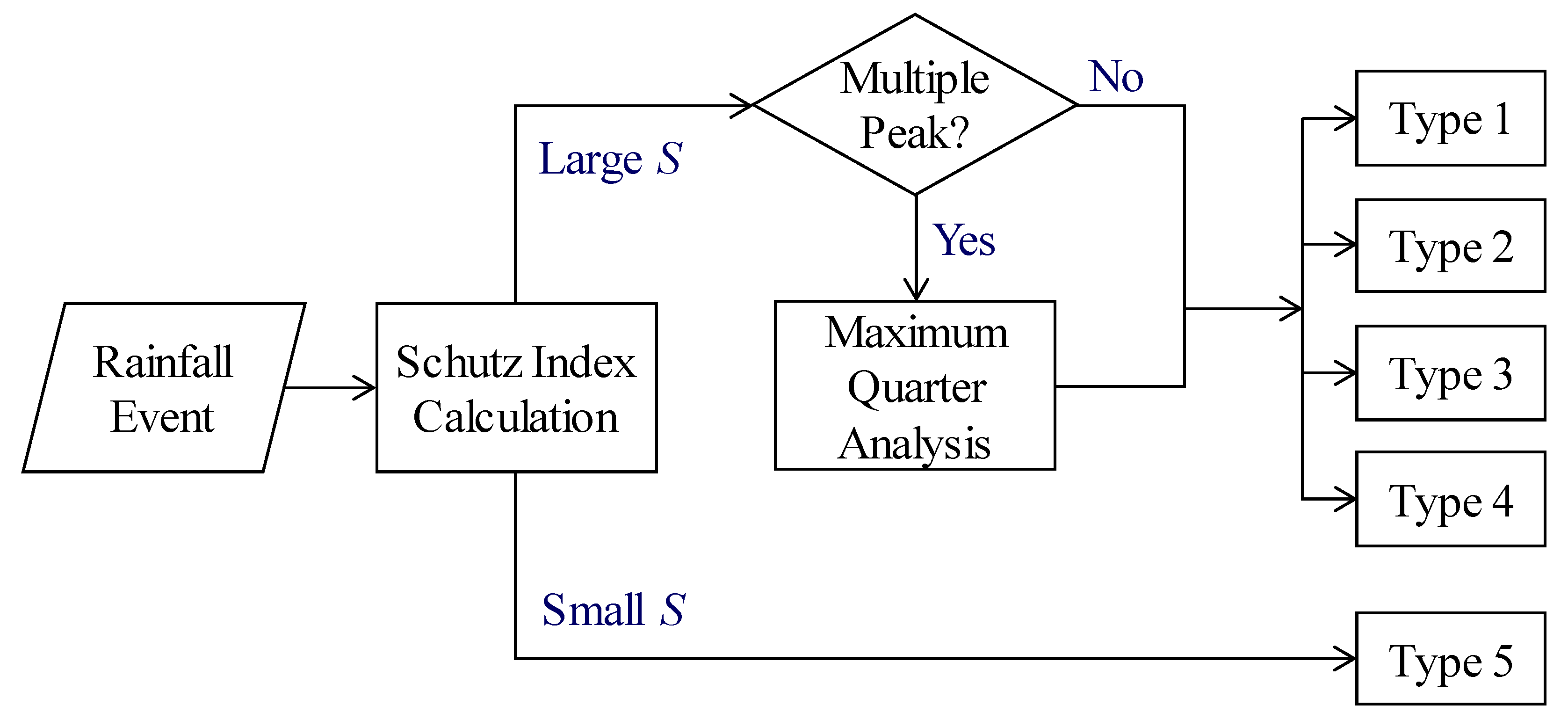
2.3. Modified Huff Rainfall Curves
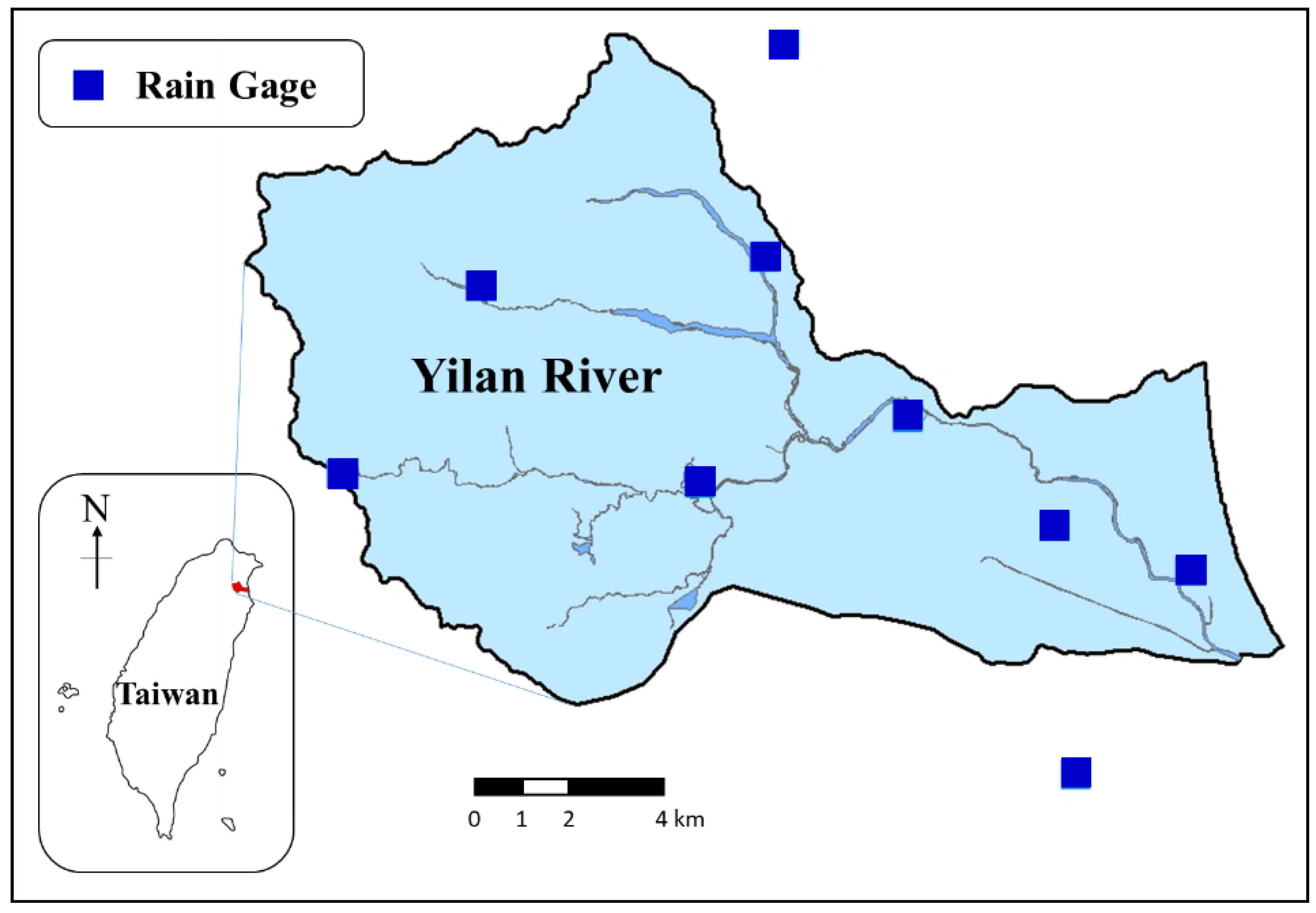
3. Study Area and Rainfall Data
4. Stochastic Rainfall-Generation Model Development
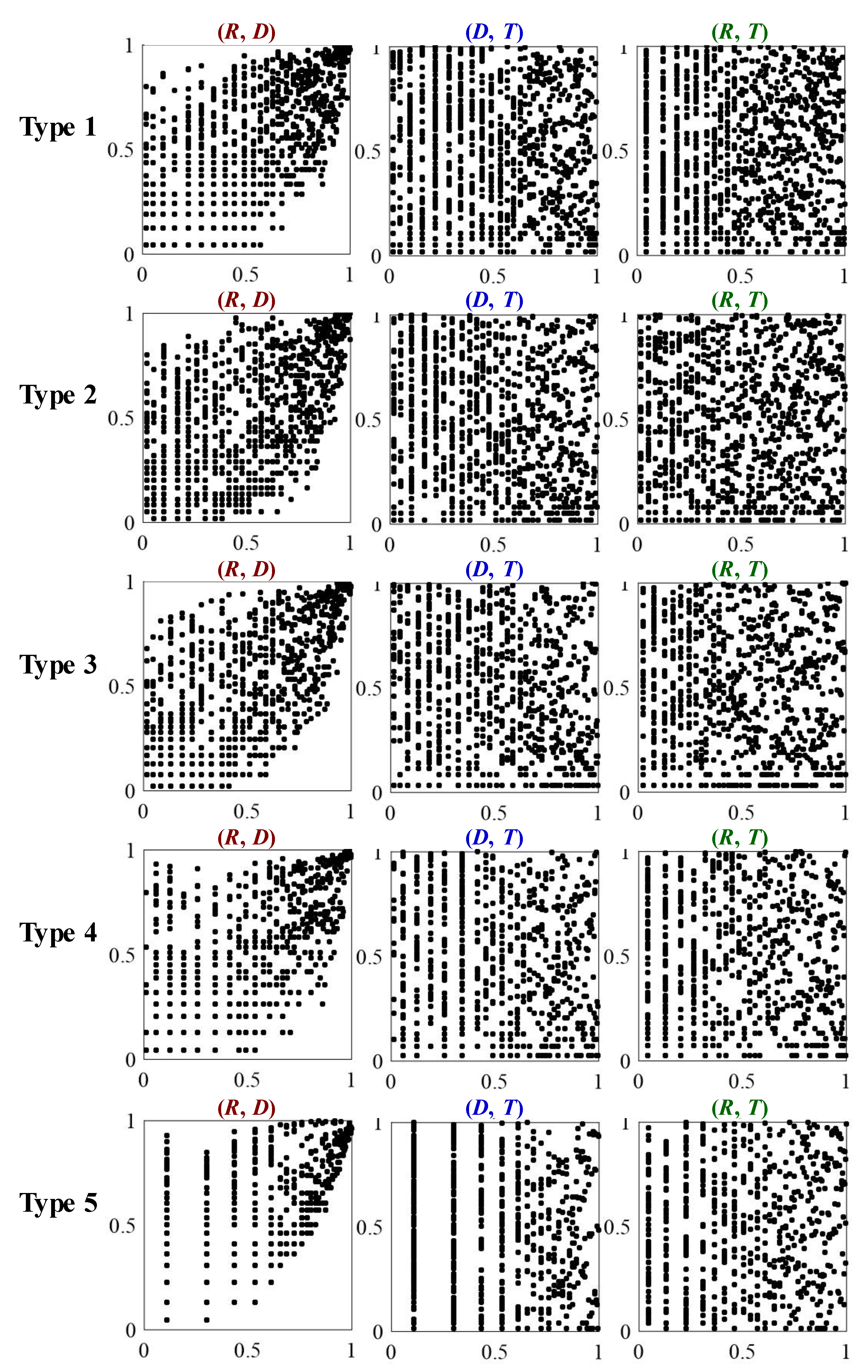
4.1. Rainfall Type
4.2. Copula Function
4.3. Procedure for Stochastic Rainfall Generation
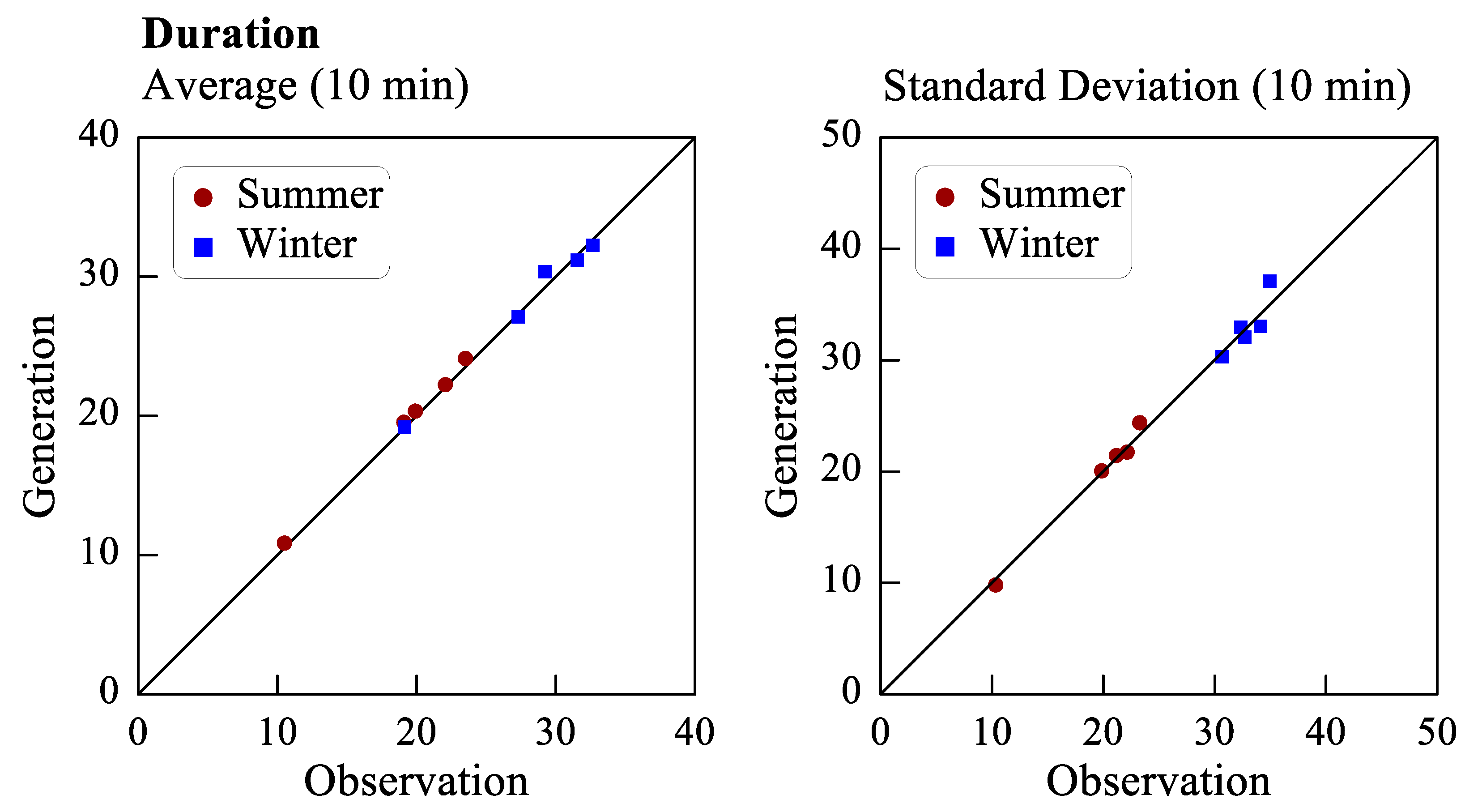
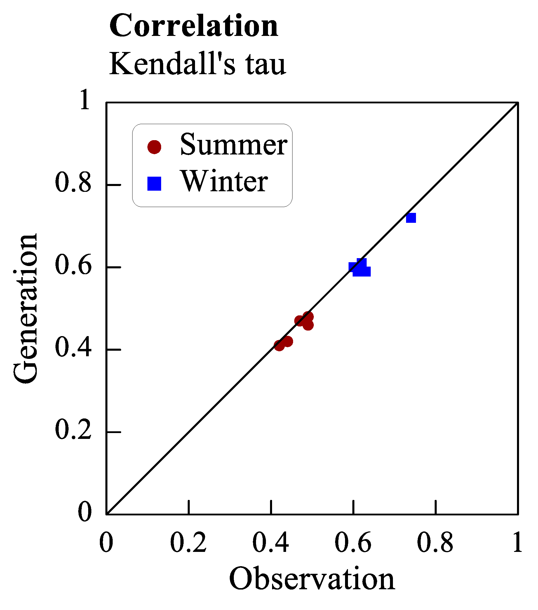
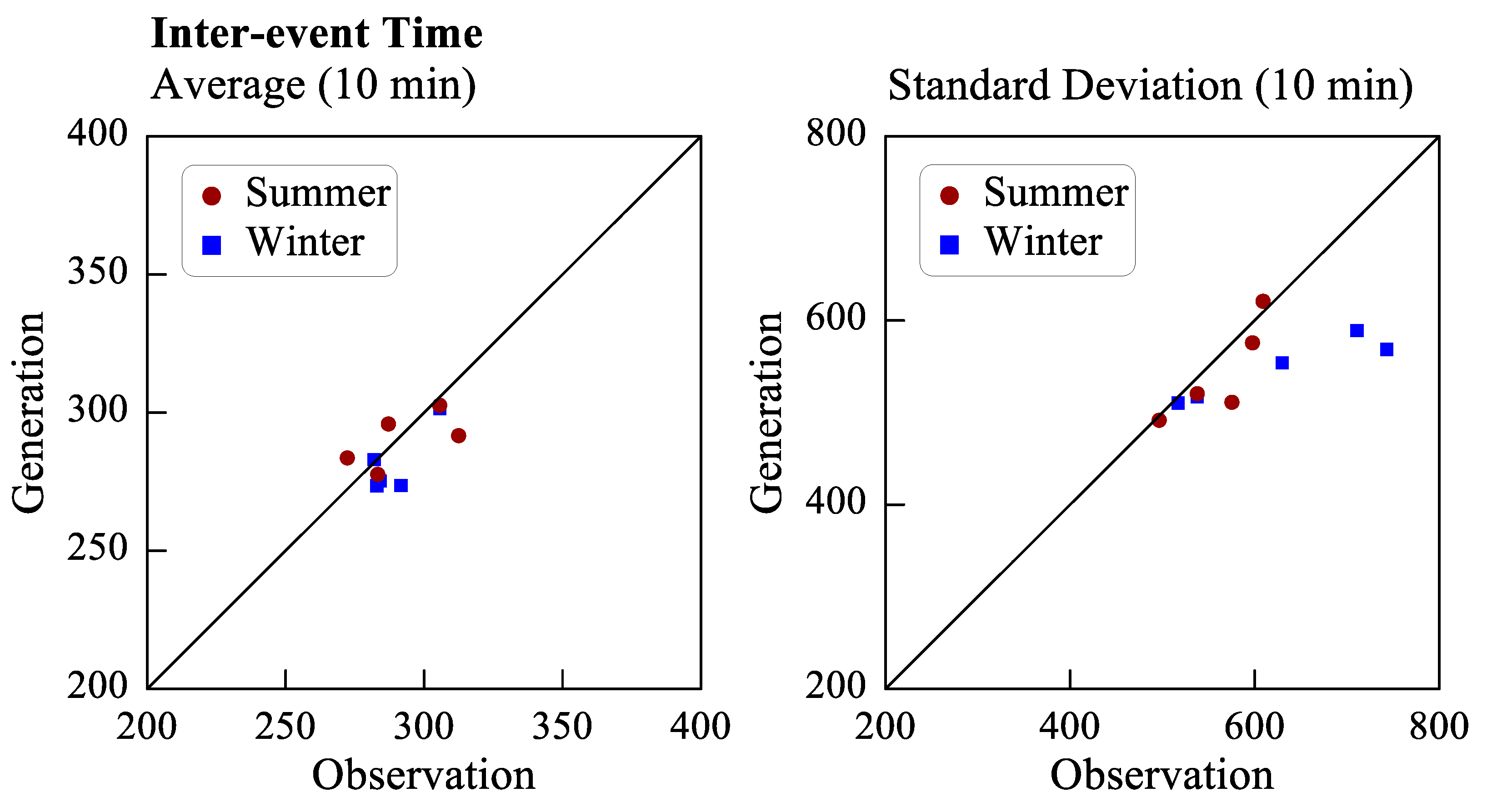
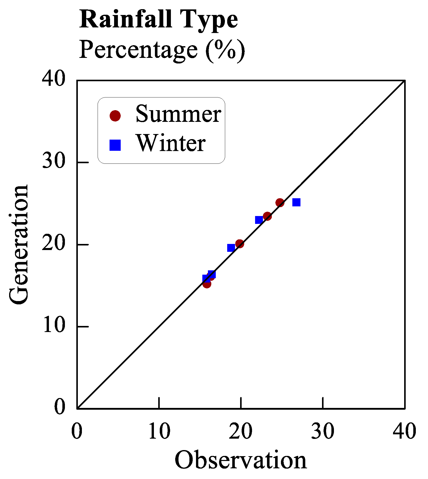
5. Results and Discussion
6. Conclusions
Author Contributions
Funding
Institutional Review Board Statement
Informed Consent Statement
Conflicts of Interest
References
- Breinl, K. Driving a lumped hydrological model with precipitation output from weather generators of different complexity. Hydrol. Sci. J. 2016, 61, 1395–1414. [Google Scholar] [CrossRef]
- Chlumecký, M.; Buchtele, J.; Richta, K. Application of random number generators in genetic algorithms to improve rainfall-runoff modelling. J. Hydrol. 2017, 553, 350–355. [Google Scholar] [CrossRef]
- Candela, A.; Brigandì, G.; Aronica, G.T. Estimation of synthetic flood design hydrographs using a distributed rainfall–runoff model coupled with a copula-based single storm rainfall generator. Nat. Hazards Earth Syst. Sci. 2014, 14, 1819–1833. [Google Scholar] [CrossRef] [Green Version]
- Winter, B.; Schneeberger, K.; Dung, N.V.; Huttenlau, M.; Achleitner, S.; Stötter, J.; Merz, B.; Vorogushyn, S. A continuous modelling approach for design flood estimation on sub-daily time scale. Hydrol. Sci. J. 2019, 64, 539–554. [Google Scholar] [CrossRef]
- Chimene, C.A.; Campos, J.N.B. The design flood under two approaches: Synthetic storm hyetograph and observed storm hyetograph. J. Appl. Water Eng. Res. 2020, 8, 171–182. [Google Scholar] [CrossRef]
- Chen, S.T.; Yu, P.S.; Tang, Y.H. Statistical downscaling of daily precipitation using support vector machines and multivariate analysis. J. Hydrol. 2010, 385, 13–22. [Google Scholar] [CrossRef]
- Yang, T.C.; Yu, P.S.; Wei, C.M.; Chen, S.T. Projection of climate change for daily precipitation: A case study in Shih-Men Reservoir catchment in Taiwan. Hydrol. Processes 2011, 25, 1342–1354. [Google Scholar] [CrossRef]
- Khazaei, M.R.; Zahabiyoun, B.; Saghafian, B. Assessment of climate change impact on floods using weather generator and continuous rainfall-runoff model. Int. J. Climatol. 2012, 32, 1997–2006. [Google Scholar] [CrossRef]
- Tukimat, N.N.A.; Syukri, N.A.; Malek, M.A. Projection the long-term ungauged rainfall using integrated Statistical Downscaling Model and Geographic Information System (SDSM-GIS) model. Heliyon 2019, 5, e02456. [Google Scholar] [CrossRef] [Green Version]
- Grimaldi, S.; Nardi, F.; Piscopia, R.; Petroselli, A.; Apollonio, C. Continuous hydrologic modelling for design simulation in small and ungauged basins: A step forward and some tests for its practical use. J. Hydrol. 2021, 595, 125664. [Google Scholar] [CrossRef]
- Katz, R.W. Precipitation as a chain-dependent process. J. Appl. Meteorol. 1977, 16, 671–676. [Google Scholar] [CrossRef] [Green Version]
- Richardson, C.W. Stochastic simulation of daily precipitation, temperature, and solar radiation. Water Resour. Res. 1981, 17, 182–190. [Google Scholar] [CrossRef]
- Westra, S.; Mehrotra, R.; Sharma, A.; Srikanthan, R. Continuous rainfall simulation: 1. A regionalized subdaily disaggregation approach. Water Resour. Res. 2012, 48, W01535. [Google Scholar] [CrossRef] [Green Version]
- De Luca, D.L.; Petroselli, A. STORAGE (STOchastic RAinfall GEnerator): A user-friendly software for generating long and high-resolution rainfall time series. Hydrology 2021, 8, 76. [Google Scholar] [CrossRef]
- Keifer, C.J.; Chu, H.H. Synthetic storm pattern for drainage design. J. Hydraul. Div. 1957, 83, 1–25. [Google Scholar] [CrossRef]
- Huff, F.A. Time distribution of rainfall in heavy storms. Water Resour. Res. 1967, 3, 1007–1019. [Google Scholar] [CrossRef]
- Yen, B.C.; Chow, V.T. Design hyetographs for small drainage structures. J. Hydraul. Div. 1980, 106, 1055–1076. [Google Scholar] [CrossRef]
- Rodriguez-Iturbe, I.; Cox, D.R.; Isham, V. Some models for rainfall based on stochastic point processes. Proc. R. Soc. London. A. Math. Phys. Sci. 1987, 410, 269–288. [Google Scholar]
- Rodriguez-Iturbe, I.; De Power, B.F.; Valdes, J.B. Rectangular pulses point process models for rainfall: Analysis of empirical data. J. Geophys. Res. Atmos. 1987, 92, 9645–9656. [Google Scholar] [CrossRef]
- Entekhabi, D.; Rodriguez-Iturbe, I.; Eagleson, P.S. Probabilistic representation of the temporal rainfall process by a modified Neyman-Scott rectangular pulses model: Parameter estimation and validation. Water Resour. Res. 1989, 25, 295–302. [Google Scholar] [CrossRef] [Green Version]
- Cowpertwait, P.S. Further developments of the Neyman-Scott clustered point process for modeling rainfall. Water Resour. Res. 1991, 27, 1431–1438. [Google Scholar] [CrossRef]
- Sørup, H.J.D.; Christensen, O.B.; Arnbjerg-Nielsen, K.; Mikkelsen, P.S. Downscaling future precipitation extremes to urban hydrology scales using a spatio-temporal Neyman–Scott weather generator. Hydrol. Earth Syst. Sci. 2016, 20, 1387–1403. [Google Scholar] [CrossRef] [Green Version]
- Cowpertwait, P.S.P.; Kilsby, C.G.; O’Connell, P.E. A space-time Neyman-Scott model of rainfall: Empirical analysis of extremes. Water Resour. Res. 2022, 38, 1131. [Google Scholar] [CrossRef]
- Lee, J.; Kim, U.; Kim, S.; Kim, J. Development and application of a rainfall temporal disaggregation method to project design rainfalls. Water 2022, 14, 1401. [Google Scholar] [CrossRef]
- De Luca, D.L.; Apollonio, C.; Petroselli, A. The benefit of continuous hydrological modelling for drought hazard assessment in small and coastal ungauged basins: A case study in Southern Italy. Climate 2022, 10, 34. [Google Scholar] [CrossRef]
- Islam, S.; Entekhabi, D.; Bras, R.L.; Rodriguez-Iturbe, I. Parameter estimation and sensitivity analysis for the modified Bartlett-Lewis rectangular pulses model of rainfall. J. Geophys. Res. Atmos. 1990, 95, 2093–2100. [Google Scholar] [CrossRef]
- Onof, C.; Wheater, H.S. Modelling of British rainfall using a random parameter Bartlett-Lewis rectangular pulse model. J. Hydrol. 1993, 149, 67–95. [Google Scholar] [CrossRef]
- Khaliq, M.N.; Cunnane, C. Modelling point rainfall occurrences with the modified Bartlett-Lewis rectangular pulses model. J. Hydrol. 1996, 180, 109–138. [Google Scholar] [CrossRef]
- Onof, C.; Wang, L.P. Modelling rainfall with a Bartlett–Lewis process: New developments. Hydrol. Earth Syst. Sci. 2020, 24, 2791–2815. [Google Scholar] [CrossRef]
- Islam, M.A.; Yu, B.; Cartwright, N. Coupling of satellite-derived precipitation products with Bartlett-Lewis model to estimate intensity-frequency-duration curves for remote areas. J. Hydrol. 2022, 609, 127743. [Google Scholar] [CrossRef]
- Rafatnejad, A.; Tavakolifar, H.; Nazif, S. Evaluation of the climate change impact on the extreme rainfall amounts using modified method of fragments for sub-daily rainfall disaggregation. Int. J. Climatol. 2022, 42, 908–927. [Google Scholar] [CrossRef]
- Huff, F.A.; Vogel, J.L. Hydrometeorology of Heavy Rainstorms in Chicago and Northeastern Illinois, Phase I—Historical Studies, Illinois State Water Survey. 1976. Available online: http://hdl.handle.net/2142/77792 (accessed on 15 May 2022).
- Huff, F.A. Time Distributions of Heavy Rainstorms in Illinois. Circular No. 173; Department of Energy and Natural Resources, State of Illi-nois. 1990. Available online: https://www.ideals.illinois.edu/bitstream/handle/2142/94492/ISWSC-173.pdf?sequence=1 (accessed on 15 May 2022).
- Yu, P.S.; Chen, S.T.; Chen, C.J.; Yang, T.C. The potential of fuzzy multi-objective model for rainfall forecasting from typhoons. Nat. Hazards 2005, 34, 131–150. [Google Scholar] [CrossRef]
- Azli, M.; Rao, A.R. Development of Huff curves for peninsular Malaysia. J. Hydrol. 2010, 388, 77–84. [Google Scholar] [CrossRef]
- Golian, S.; Saghafian, B.; Maknoon, R. Derivation of probabilistic thresholds of spatially distributed rainfall for flood forecasting. Water Resour. Manag. 2010, 24, 3547–3559. [Google Scholar] [CrossRef]
- Chen, S.T. Multiclass support vector classification to estimate typhoon rainfall distribution. Disaster Adv. 2013, 6, 110–121. [Google Scholar]
- Dolšak, D.; Bezak, N.; Šraj, M. Temporal characteristics of rainfall events under three climate types in Slovenia. J. Hydrol. 2016, 541, 1395–1405. [Google Scholar] [CrossRef]
- Wartalska, K.; Kaźmierczak, B.; Nowakowska, M.; Kotowski, A. Analysis of hyetographs for drainage system modeling. Water 2020, 12, 149. [Google Scholar] [CrossRef] [Green Version]
- Dunkerley, D. Regional rainfall regimes affect the sensitivity of the Huff quartile classification to the method of event delineation. Water 2022, 14, 1047. [Google Scholar] [CrossRef]
- Sklar, M. Fonctions de repartition an dimensions et leurs marges. Publ. Inst. Statist. Univ. Paris 1959, 8, 229–231. [Google Scholar]
- De Michele, C.; Salvadori, G. A generalized Pareto intensity-duration model of storm rainfall exploiting 2-copulas. J. Geophys. Res. Atmos. 2003, 108, 4067. [Google Scholar] [CrossRef]
- Favre, A.C.; El Adlouni, S.; Perreault, L.; Thiémonge, N.; Bobée, B. Multivariate hydrological frequency analysis using copulas. Water Resour. Res. 2004, 40, W01101. [Google Scholar] [CrossRef] [Green Version]
- Kao, S.C.; Chang, N.B. Copula-based flood frequency analysis at ungauged basin confluences: Nashville, Tennessee. J. Hydrol. Eng. 2012, 17, 790–799. [Google Scholar] [CrossRef]
- Dodangeh, E.; Singh, V.P.; Pham, B.T.; Yin, J.; Yang, G.; Mosavi, A. Flood frequency analysis of interconnected Rivers by copulas. Water Resour. Manag. 2020, 34, 3533–3549. [Google Scholar] [CrossRef]
- Pathak, A.A.; Dodamani, B.M. Connection between meteorological and groundwater drought with copula-based bivariate frequency analysis. J. Hydrol. Eng. 2021, 26, 05021015. [Google Scholar] [CrossRef]
- Razmkhah, H.; Fararouie, A.; Ravari, A.R. Multivariate flood frequency analysis using bivariate copula functions. Water Resour. Manag. 2022, 36, 729–743. [Google Scholar] [CrossRef]
- Jang, J.H.; Chang, T.H. Flood risk estimation under the compound influence of rainfall and tide. J. Hydrol. 2022, 606, 127446. [Google Scholar] [CrossRef]
- Genest, C.; Rivest, L.P. On the multivariate probability integral transformation. Stat. Probab. Lett. 2001, 53, 391–399. [Google Scholar] [CrossRef]
- Kao, S.C.; Govindaraju, R.S. Trivariate statistical analysis of extreme rainfall events via the Plackett family of copulas. Water Resour. Res. 2008, 44, W02415. [Google Scholar] [CrossRef]
- Kao, S.C.; Govindaraju, R.S. A copula-based joint deficit index for droughts. J. Hydrol. 2010, 380, 121–134. [Google Scholar] [CrossRef]
- Amirataee, B.; Montaseri, M.; Rezaie, H. An advanced data collection procedure in bivariate drought frequency analysis. Hydrol. Processes 2020, 34, 4067–4082. [Google Scholar] [CrossRef]
- Salvadori, G.; De Michele, C. Frequency analysis via copulas: Theoretical aspects and applications to hydrological events. Water Resour. Res. 2004, 40, W12511. [Google Scholar] [CrossRef]
- Salvadori, G.; De Michele, C. On the use of copulas in hydrology: Theory and practice. J. Hydrol. Eng. 2007, 12, 369–380. [Google Scholar] [CrossRef]
- Genest, C.; Favre, A.C. Everything you always wanted to know about copula modeling but were afraid to ask. J. Hydrol. Eng. 2007, 12, 347–368. [Google Scholar] [CrossRef]
- Gao, C.; Xu, Y.P.; Zhu, Q.; Bai, Z.; Liu, L. Stochastic generation of daily rainfall events: A single-site rainfall model with copula-based joint simulation of rainfall characteristics and classification and simulation of rainfall patterns. J. Hydrol. 2018, 564, 41–58. [Google Scholar] [CrossRef]
- Vandenberghe, S.; Verhoest, N.E.C.; De Baets, B. Properties and performance of a copula-based design storm generator. In Proceedings of the International workshop: Advances in Statistical Hydrology, Taormina, Italy, 23–25 May 2010. [Google Scholar]
- Schutz, R.R. On the measurement of income inequality. Am. Econ. Rev. 1951, 41, 107–122. [Google Scholar]
- Lorenz, M.O. Methods of measuring the concentration of wealth. Publ. Am. Stat. Assoc. 1905, 9, 209–219. [Google Scholar] [CrossRef]
- Cameron, D.; Beven, K.; Naden, P. Flood frequency estimation by continuous simulation under climate change (with uncertainty). Hydrol. Earth Syst. Sci. 2020, 4, 393–405. [Google Scholar] [CrossRef]
- Sharafati, A.; Zahabiyoun, B. Stochastic generation of storm pattern. Life Sci. J. 2013, 10, 1575–1583. [Google Scholar]
- Bonta, J.V.; Rao, A.R. Factors affecting the identification of independent storm events. J. Hydrol. 1988, 98, 275–293. [Google Scholar] [CrossRef]
- Vernieuwe, H.; Vandenberghe, S.; De Baets, B.; Verhoest, N. A continuous rainfall model based on vine copulas. Hydrol. Earth Syst. Sci. 2015, 19, 2685–2699. [Google Scholar] [CrossRef] [Green Version]
- Bonta, J.V.; Shahalam, A. Cumulative storm rainfall distributions: Comparison of Huff curves. J. Hydrol. 2003, 42, 65–74. [Google Scholar]


| Copula | Function | Parameter Space | |
|---|---|---|---|
| Clayton | |||
| Frank | |||
| Gumbel |
| Summer Season | Winter Season | |||
|---|---|---|---|---|
| Number of Events | Percentage (%) | Number of Events | Percentage (%) | |
| Type 1 | 1069 | 24.76 | 869 | 26.77 |
| Type 2 | 1003 | 23.24 | 721 | 22.21 |
| Type 3 | 857 | 19.85 | 610 | 18.79 |
| Type 4 | 704 | 16.31 | 534 | 16.45 |
| Type 5 | 684 | 15.84 | 512 | 15.78 |
| Schutz index | 0.29 | 0.30 | ||
| Summer Season | Winter Season | |||||||
|---|---|---|---|---|---|---|---|---|
| Clayton | Frank | Gumbel | Clayton | Frank | Gumbel | |||
| Type 1 | 0.487 | 1.901 | 5.510 | 1.950 | 0.602 | 3.021 | 7.975 | 2.511 |
| Type 2 | 0.417 | 1.428 | 4.394 | 1.714 | 0.633 | 3.455 | 8.893 | 2.727 |
| Type 3 | 0.465 | 1.739 | 5.136 | 1.870 | 0.613 | 3.161 | 8.273 | 2.581 |
| Type 4 | 0.436 | 1.546 | 4.680 | 1.773 | 0.623 | 3.307 | 8.581 | 2.653 |
| Type 5 | 0.490 | 1.920 | 5.553 | 1.960 | 0.743 | 5.785 | 13.70 | 3.892 |
| Summer Season | Winter Season | |||||
|---|---|---|---|---|---|---|
| Clayton | Frank | Gumbel | Clayton | Frank | Gumbel | |
| Type 1 | 0.030 | 0.027 | 0.028 | 0.038 | 0.036 | 0.037 |
| Type 2 | 0.024 | 0.019 | 0.018 | 0.026 | 0.024 | 0.025 |
| Type 3 | 0.026 | 0.020 | 0.020 | 0.023 | 0.022 | 0.022 |
| Type 4 | 0.034 | 0.030 | 0.031 | 0.042 | 0.040 | 0.041 |
| Type 5 | 0.059 | 0.059 | 0.060 | 0.052 | 0.052 | 0.052 |
Publisher’s Note: MDPI stays neutral with regard to jurisdictional claims in published maps and institutional affiliations. |
© 2022 by the authors. Licensee MDPI, Basel, Switzerland. This article is an open access article distributed under the terms and conditions of the Creative Commons Attribution (CC BY) license (https://creativecommons.org/licenses/by/4.0/).
Share and Cite
Nguyen, D.T.; Chen, S.-T. Generating Continuous Rainfall Time Series with High Temporal Resolution by Using a Stochastic Rainfall Generator with a Copula and Modified Huff Rainfall Curves. Water 2022, 14, 2123. https://doi.org/10.3390/w14132123
Nguyen DT, Chen S-T. Generating Continuous Rainfall Time Series with High Temporal Resolution by Using a Stochastic Rainfall Generator with a Copula and Modified Huff Rainfall Curves. Water. 2022; 14(13):2123. https://doi.org/10.3390/w14132123
Chicago/Turabian StyleNguyen, Dinh Ty, and Shien-Tsung Chen. 2022. "Generating Continuous Rainfall Time Series with High Temporal Resolution by Using a Stochastic Rainfall Generator with a Copula and Modified Huff Rainfall Curves" Water 14, no. 13: 2123. https://doi.org/10.3390/w14132123