Hydrodynamic Border Irrigation Model: Comparison of Infiltration Equations

Abstract

The variation in moisture content between subsequent irrigations determines the use of infiltration equations that contain representative physical parameters of the soil when irrigation begins. This study analyzes the reliability of the hydrodynamic model to simulate the advanced phase in border irrigation. For the solution of the hydrodynamic model, a Lagrangian scheme in implicit finite differences is used, while for infiltration, the Kostiakov equation and the Green and Ampt equation are used and compared. The latter was solved using the Newton–Raphson method due to its implicit nature. The models were validated, and unknown parameters were optimized using experimental data available in the literature and the Levenberg–Marquardt method. The results show that it is necessary to use infiltration equations based on soil parameters, because in subsequent irrigations, the initial conditions change, modifying the advance curve in border irrigation. From the coupling of both equations, it is shown that the empirical Kostiakov equation is only representative for a specific irrigation event, while with the Green and Ampt equations, the subsequent irrigations can be modeled, and the advance/infiltration process can be observed in detail.

1. Introduction

More than 90% of the irrigated area worldwide uses the surface irrigation method, with the main disadvantage being low yield due to poor design and operation [1,2].

In surface irrigation, the water is distributed throughout the soil profile, making it necessary to study and develop methodologies to model the water infiltration and redistribution processes [3]. The infiltration process varies over time, and with the characteristics of the plot, it affects the surface’s flow by making it unstable and spatially variable [4].

There are three distinguishable phases that occur during the surface irrigation event, the advanced phase, the storage phase, and the recession phase, which together are studied with a variety of models to understand the phenomenon [5].

According to the Saint-Venant equations, formed by the continuity equation and the momentum equation, the mathematical models for simulating surface irrigation are mainly classified into four groups [6]: the volume balance model, the kinematic wave model, the zero-inertia model, and the hydrodynamic model.

Using the volume balance model and a hybrid metaheuristic solution algorithm, surface irrigation can be designed and evaluated by coupling the Kostiakov–Lewis infiltration equation and a potential function in the advance phase [1]. Another solution method is based on solving the Lewis–Milne integral for the advance phase [7].

In combination with the kinematic wave model, the Kostiakov–Lewis equation is generally used to describe the soil’s water flow [8]. However, with this model, it is not possible to incorporate downstream boundary conditions that alter the upstream flow, such as a furrow or a closed border at the end. This disadvantage was eliminated with a simplified method to distribute the water in the final part of the furrow or border, and it was also improved by using the infiltration equation of Green and Ampt based on the physical parameters of the soil [9].

The border irrigation modeling can be carried out by the zero-inertia model that is based on a Lagrangian scheme in finite differences for surface flow, while for the description of the flow of water in the soil, it uses the Kostiakov equation [10] and is adapted for furrow irrigation [11]. The WinSRFR software uses the zero-inertia model coupled with infiltration equations such as those of Richards, Green and Ampt, Kostiakov, and Kostiakov–Lewis [12]. However, with this model, it is not possible to describe the irrigation with furrow or border lengths greater than 300 m, because the model does not introduce inertial errors and the output data do not fit the experimental data correctly.

The hydrodynamic model has been used less frequently. Software such as SIRMOD [13] and SISCO [14] has been developed through a finite difference scheme of rectangular cells and, for the subsurface flow of water, they use the Kostiakov–Lewis equation, while other models use the Kostiakov equation and a solution method based on an explicit algorithm with a MacCormack scheme [15]. Other models use infiltration equations that are based on physically based parameters, such as that of Green and Ampt [3,16], where the moisture profile is assumed to be constant, and the models that incorporate an analytical solution for the infiltration in a soil with a shallow water table for the advance phase of border irrigation [17].

The main differences between the models are the number of parameters in the equations, the solution methods, and the coupled infiltration equations. It is important to mention that most of the solutions presented mainly use the Kostiakov and Kostiakov–Lewis equations. However, these functions do not include the use of physical parameters that are representative of the soil in their variables and that can be adapted to vary them temporarily without having to perform so many irrigation tests.

In this article, we describe the comparison of two of the most-used infiltration equations to model surface irrigation, presenting a solution based on the complete hydrodynamic model of the Saint-Venant equations using a finite difference Lagrangian scheme for the solution of the advance phase.

2. Model Development

In this work, the complete hydrodynamic model was used for the surface flow, and for the subsurface flow a comparison between two infiltration equations was made. The continuity equation for a border irrigation was expressed as follows:

$$\frac{\partial \mathrm{h}}{\partial \mathrm{t}}+\frac{\partial \mathrm{q}}{\partial \mathrm{x}}+\frac{\partial \mathrm{I}}{\partial \mathrm{t}}=0$$

(1)

while the momentum equation was written in the following recommended form for border irrigation [17]:

$${\mathrm{h}}^2\frac{\partial \mathrm{q}}{\partial \mathrm{t}}+2\mathrm{h}\mathrm{q}\frac{\partial \mathrm{q}}{\partial \mathrm{x}}+\left(\mathrm{g}{\mathrm{h}}^3-{\mathrm{q}}^2\right)\frac{\partial \mathrm{h}}{\partial \mathrm{x}}+\mathrm{g}{\mathrm{h}}^3\left(\mathrm{J}-{\mathrm{J}}_{\mathrm{o}}\right)+\mathsf{\beta }\mathrm{q}\mathrm{h}\frac{\partial \mathrm{I}}{\partial \mathrm{t}}=0$$

(2)

where h is the water depth, q(x,t) = U(x,t)h(x,t) is the discharge per unit width of the border or the unitary discharge, x is the spatial coordinate in the main direction of the water movement in the border, t is the time, U is the mean velocity, β = U_IX/U is a dimensionless parameter where U_IX is the projection in the direction of the output velocity of the water mass due to the infiltration, V_I = ∂I(x,t)/∂t is the infiltration flow, that is, the water volume infiltrated per unit width per unit length of the border, I is the infiltrated depth, g is gravitational acceleration, J_o is the topographic slope, and J is the friction slope that can be determined by the fractal law of hydraulic resistance [3]:

$$\mathrm{q}=\mathrm{k}\mathsf{\nu }{\left(\frac{{\mathrm{h}}^3\mathrm{J}\mathrm{g}}{{\mathsf{\nu }}^2}\right)}^{\mathrm{d}}$$

(3)

where ν is the coefficient of kinematic viscosity, k is a dimensionless factor that includes the effects of the roughness of the soil surface, and exponent d is an exponent such that 1/2 ≤ d ≤ 1 in a manner that d = 1/2 corresponds to the Chézy turbulent regime and d = 1 to the Poiseuille regime.

The two methods for calculating the cumulative infiltration are the empiric Kostiakov equation and the Green and Ampt equation. The Kostiakov equation is described as follows [18]:

$$\mathrm{I}=\mathsf{\kappa }{\mathsf{\tau }}^{\mathrm{\alpha }}$$

(4)

where τ is the opportunity time, and κ and α are the empirical infiltration parameters.

The Green and Ampt equation [19] is established from the continuity equation and Darcy’s law based on the following hypotheses: (a) the initial moisture profile in a soil column is uniform θ = θ_o; (b) water pressure at the soil surface is hydrostatic, ψ ≥ 0, where h is the water depth; (c) there is a well-defined wetting front characterized by negative pressure: ψ = −h_f < 0, where h_f is the suction at the wetting front; (d) the region between the soil surface and the wetting front is completely saturated (plug flow), θ = θ_s and K = K_s, where K_s is the hydraulic conductivity at saturation, that is, the value of the hydraulic conductivity of Darcy’s law corresponding to the volumetric saturation content of water:

$$\mathrm{I}={\mathrm{K}}_{\mathrm{s}}\mathrm{t}+\lambda \ln \left(1+\frac{\mathrm{I}}{\lambda }\right), \lambda =\left(\mathrm{h}+{\mathrm{h}}_{\mathrm{f}}\right)\left({\mathsf{\theta }}_{\mathrm{s}}-{\mathsf{\theta }}_{\mathrm{o}}\right)$$

(5)

where t is the time, θ_s is the soil moisture at saturation, and θ_o is the initial moisture.

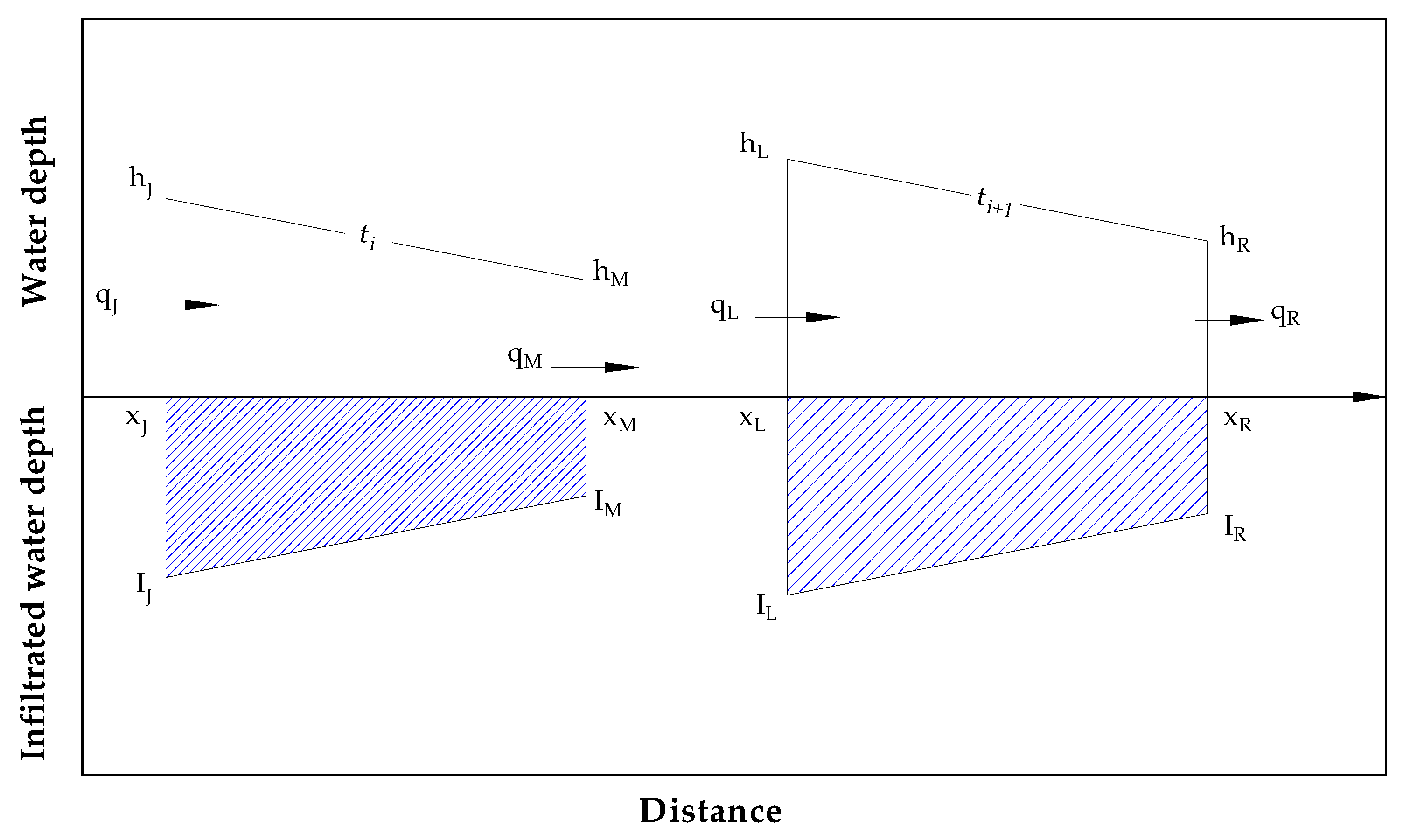
For the discretization of Equations (1) and (2), a finite-difference Lagrangian scheme was used for its solution [3,17]. Figure 1 shows the flows and depths of water on the surface as infiltrates at times t_i and t_i+1 with the subscripts J, M, L, and R to identify the time step and the boundary conditions in a specific cell.

2.1. Discretization of the Saint-Venant Equation

Average weighting factors in time and space, denoted by ω and φ, respectively, were used due to the non-linearity of the upper and lower limits [20]. The common limits of these weighting factors are 0 ≤ ω ≤ 1 and 0 ≤ φ ≤ 1.

The discrete form of the continuity equation from the schematic in Figure 1 is as follows.

$$\begin{array}{l}\left[\mathsf{\omega }\left({\mathrm{q}}_{\mathrm{L}}-{\mathrm{q}}_{\mathrm{R}}\right)+\left(1-\mathsf{\omega }\right)\left({\mathrm{q}}_{\mathrm{J}}-{\mathrm{q}}_{\mathrm{M}}\right)\right]\mathsf{\delta }\mathrm{t}\\ -\left[\mathsf{\omega }\left({\mathrm{h}}_{\mathrm{L}}+{\mathrm{I}}_{\mathrm{L}}\right)+\left(1-\mathsf{\omega }\right)\left({\mathrm{h}}_{\mathrm{J}}+{\mathrm{I}}_{\mathrm{J}}\right)\right]\left({\mathrm{x}}_{\mathrm{L}}-{\mathrm{x}}_{\mathrm{J}}\right)\\ +\left[\mathsf{\omega }\left({\mathrm{h}}_{\mathrm{R}}+{\mathrm{I}}_{\mathrm{R}}\right)+\left(1-\mathsf{\omega }\right)\left({\mathrm{h}}_{\mathrm{M}}+{\mathrm{I}}_{\mathrm{M}}\right)\right]\left({\mathrm{x}}_{\mathrm{R}}-{\mathrm{x}}_{\mathrm{M}}\right)\\ +\left[\mathsf{\phi }\left({\mathrm{h}}_{\mathrm{J}}+{\mathrm{I}}_{\mathrm{J}}\right)+\left(1-\mathsf{\phi }\right)\left({\mathrm{h}}_{\mathrm{M}}+{\mathrm{I}}_{\mathrm{M}}\right)\right]\left({\mathrm{x}}_{\mathrm{M}}-{\mathrm{x}}_{\mathrm{J}}\right)\\ -\left[\mathsf{\phi }\left({\mathrm{h}}_{\mathrm{L}}+{\mathrm{I}}_{\mathrm{L}}\right)+\left(1-\mathsf{\phi }\right)\left({\mathrm{h}}_{\mathrm{R}}+{\mathrm{I}}_{\mathrm{R}}\right)\right]\left({\mathrm{x}}_{\mathrm{R}}-{\mathrm{x}}_{\mathrm{L}}\right)=\mathrm{R}\mathrm{c}\end{array}$$

(6)

The discretization of the momentum equation is governed by the following hypotheses [3,21]: (a) A Eulerian discretization (rectangular cells) is considered for the time derivatives and (b) an average friction slope is taken into account from the average flow and water-depth coefficients. With the above, the discrete form of Equation (2) is written as follows:

$$\begin{array}{l}{\overline{\mathrm{h}}}^2\left\{\left[\mathsf{\phi }{\mathrm{q}}_{\mathrm{L}}+\left(1-\mathsf{\phi }\right){\mathrm{q}}_{\mathrm{R}}\right]\left({\mathrm{x}}_{\mathrm{R}}-{\mathrm{x}}_{\mathrm{L}}\right)-\left[\mathsf{\phi }{\mathrm{q}}_{\mathrm{J}}+\left(1-\mathsf{\phi }\right){\mathrm{q}}_{\mathrm{M}}\right]\left({\mathrm{x}}_{\mathrm{M}}-{\mathrm{x}}_{\mathrm{J}}\right)\right\}\\ +2\overline{\mathrm{h}}\overline{\mathrm{q}}\left[\mathsf{\omega }\left({\mathrm{q}}_{\mathrm{R}}-{\mathrm{q}}_{\mathrm{L}}\right)+\left(1-\mathsf{\omega }\right)\left({\mathrm{q}}_{\mathrm{M}}-{\mathrm{q}}_{\mathrm{J}}\right)\right]\mathsf{\delta }\mathrm{t}\\ +\left(\mathrm{g}{\overline{\mathrm{h}}}^3-{\overline{\mathrm{q}}}^2\right)\left[\mathsf{\omega }\left({\mathrm{h}}_{\mathrm{R}}-{\mathrm{h}}_{\mathrm{L}}\right)+\left(1-\mathsf{\omega }\right)\left({\mathrm{h}}_{\mathrm{M}}-{\mathrm{h}}_{\mathrm{J}}\right)\right]\mathsf{\delta }\mathrm{t}\\ +\mathrm{g}{\overline{\mathrm{h}}}^3\left(\overline{\mathrm{J}}-{\mathrm{J}}_{\mathrm{o}}\right)\left[\mathsf{\omega }\left({\mathrm{x}}_{\mathrm{R}}-{\mathrm{x}}_{\mathrm{L}}\right)+\left(1-\mathsf{\omega }\right)\left({\mathrm{x}}_{\mathrm{M}}-{\mathrm{x}}_{\mathrm{J}}\right)\right]\mathsf{\delta }\mathrm{t}\\ +\mathsf{\beta }\overline{\mathrm{q}}\overline{\mathrm{h}}\left\{\left[\mathsf{\phi }{\mathrm{I}}_{\mathrm{L}}+\left(1-\mathsf{\phi }\right){\mathrm{I}}_{\mathrm{R}}\right]\left({\mathrm{x}}_{\mathrm{R}}-{\mathrm{x}}_{\mathrm{L}}\right)-\left[\mathsf{\phi }{\mathrm{I}}_{\mathrm{J}}+\left(1-\mathsf{\phi }\right){\mathrm{I}}_{\mathrm{M}}\right]\left({\mathrm{x}}_{\mathrm{M}}-{\mathrm{x}}_{\mathrm{J}}\right)\right\}=\mathrm{R}\mathrm{m}\end{array}$$

(7)

where the coefficients $\overline{\mathrm{h}}$ = ω[(1 − φ)h_R + φh_L] + (1 − ω)[(1 − φ)h_M + φh_J] and $\overline{\mathrm{q}}$ = ω[(1 − φ)q_R + φq_L] + (1 − ω)[(1 − φ)q_M + φq_J] consider the values at the border of each calculation cell in a time step. With these coefficients, the average friction slope is $\overline{\mathrm{J}}$ = ν²($\overline{\mathrm{q}}$/k ν)^1/d/g${\overline{\mathrm{h}}}^3$. Rc and Rm are the residuals of the continuity and momentum equations, respectively.

2.2. Solution Procedure

In order to solve the equations, the Newton–Raphson method was used, which requires the calculation of the function derivatives with respect to the unknown values h_L, q_L, h_R, and q_R, resulting in the equation system shown in Equation (8).

$$\left[\begin{array}{cccccccccccccc}-{\mathrm{S}}_1& 1& & & & & & & & & & & & \\ \frac{\partial \mathrm{R}{\mathrm{c}}_1}{\partial {\mathrm{h}}_{\mathrm{L}}}& \frac{\partial \mathrm{R}{\mathrm{c}}_1}{\partial {\mathrm{q}}_{\mathrm{L}}}& \frac{\partial \mathrm{R}{\mathrm{c}}_1}{\partial {\mathrm{h}}_{\mathrm{R}}}& \frac{\partial \mathrm{R}{\mathrm{c}}_1}{\partial {\mathrm{q}}_{\mathrm{R}}}& & & & & & & & & & \\ \frac{\partial \mathrm{R}{\mathrm{m}}_1}{\partial {\mathrm{h}}_{\mathrm{L}}}& \frac{\partial \mathrm{R}{\mathrm{m}}_1}{\partial {\mathrm{q}}_{\mathrm{L}}}& \frac{\partial \mathrm{R}{\mathrm{m}}_1}{\partial {\mathrm{h}}_{\mathrm{R}}}& \frac{\partial \mathrm{R}{\mathrm{m}}_1}{\partial {\mathrm{q}}_{\mathrm{R}}}& & & & & & & & & & \\ & & \frac{\partial \mathrm{R}{\mathrm{c}}_2}{\partial {\mathrm{h}}_{\mathrm{L}}}& \frac{\partial \mathrm{R}{\mathrm{c}}_2}{\partial {\mathrm{q}}_{\mathrm{L}}}& \frac{\partial \mathrm{R}{\mathrm{c}}_2}{\partial {\mathrm{h}}_{\mathrm{R}}}& \frac{\partial \mathrm{R}{\mathrm{c}}_2}{\partial {\mathrm{q}}_{\mathrm{R}}}& & & & & & & & \\ & & \frac{\partial \mathrm{R}{\mathrm{m}}_2}{\partial {\mathrm{h}}_{\mathrm{L}}}& \frac{\partial \mathrm{R}{\mathrm{m}}_2}{\partial {\mathrm{q}}_{\mathrm{L}}}& \frac{\partial \mathrm{R}{\mathrm{m}}_2}{\partial {\mathrm{h}}_{\mathrm{R}}}& \frac{\partial \mathrm{R}{\mathrm{m}}_2}{\partial {\mathrm{q}}_{\mathrm{R}}}& & & & & & & & \\ & & & & ·& ·& ·& ·& & & & & & \\ & & & & ·& ·& ·& ·& & & & & & \\ & & & & & & ·& ·& ·& ·& & & & \\ & & & & & & ·& ·& ·& ·& & & & \\ & & & & & & & & \frac{\partial \mathrm{R}{\mathrm{c}}_{\mathrm{N}-1}}{\partial {\mathrm{h}}_{\mathrm{L}}}& \frac{\partial \mathrm{R}{\mathrm{c}}_{\mathrm{N}-1}}{\partial {\mathrm{q}}_{\mathrm{L}}}& \frac{\partial \mathrm{R}{\mathrm{c}}_{\mathrm{N}-1}}{\partial {\mathrm{h}}_{\mathrm{R}}}& \frac{\partial \mathrm{R}{\mathrm{c}}_{\mathrm{N}-1}}{\partial {\mathrm{q}}_{\mathrm{R}}}& & \\ & & & & & & & & \frac{\partial \mathrm{R}{\mathrm{m}}_{\mathrm{N}-1}}{\partial {\mathrm{h}}_{\mathrm{L}}}& \frac{\partial \mathrm{R}{\mathrm{m}}_{\mathrm{N}-1}}{\partial {\mathrm{q}}_{\mathrm{L}}}& \frac{\partial \mathrm{R}{\mathrm{m}}_{\mathrm{N}-1}}{\partial {\mathrm{h}}_{\mathrm{R}}}& \frac{\partial \mathrm{R}{\mathrm{m}}_{\mathrm{N}-1}}{\partial {\mathrm{q}}_{\mathrm{R}}}& & \\ & & & & & & & & & & \frac{\partial \mathrm{R}{\mathrm{c}}_{\mathrm{N}}}{\partial {\mathrm{h}}_{\mathrm{L}}}& \frac{\partial \mathrm{R}{\mathrm{c}}_{\mathrm{N}}}{\partial {\mathrm{q}}_{\mathrm{L}}}& \frac{\partial \mathrm{R}{\mathrm{c}}_{\mathrm{N}}}{\partial {\mathrm{h}}_{\mathrm{R}}}& \frac{\partial \mathrm{R}{\mathrm{c}}_{\mathrm{N}}}{\partial {\mathrm{x}}_{\mathrm{N}}}\\ & & & & & & & & & & \frac{\partial \mathrm{R}{\mathrm{m}}_{\mathrm{N}}}{\partial {\mathrm{h}}_{\mathrm{L}}}& \frac{\partial \mathrm{R}{\mathrm{m}}_{\mathrm{N}}}{\partial {\mathrm{q}}_{\mathrm{L}}}& \frac{\partial \mathrm{R}{\mathrm{m}}_{\mathrm{N}}}{\partial {\mathrm{h}}_{\mathrm{R}}}& \frac{\partial \mathrm{R}{\mathrm{m}}_{\mathrm{N}}}{\partial {\mathrm{x}}_{\mathrm{N}}}\\ & & & & & & & & & & & & -{\mathrm{S}}_{\mathrm{N}+1}& 1\end{array}\right] \left[\begin{array}{c}\mathsf{\delta }{\mathrm{h}}_0\\ \mathsf{\delta }{\mathrm{q}}_0\\ \mathsf{\delta }{\mathrm{h}}_1\\ \mathsf{\delta }{\mathrm{q}}_1\\ \mathsf{\delta }{\mathrm{h}}_2\\ \mathsf{\delta }{\mathrm{q}}_2\\ ·\\ ·\\ \mathsf{\delta }{\mathrm{h}}_{\mathrm{N}-2}\\ \mathsf{\delta }{\mathrm{q}}_{\mathrm{N}-2}\\ \mathsf{\delta }{\mathrm{h}}_{\mathrm{N}-1}\\ \mathsf{\delta }{\mathrm{q}}_{\mathrm{N}-1}\\ \mathsf{\delta }{\mathrm{h}}_{\mathrm{N}}\\ \mathsf{\delta }\mathsf{\delta }\end{array}\right]=\left[\begin{array}{c}{\mathrm{T}}_1\\ \mathrm{R}{\mathrm{c}}_1\\ \mathrm{R}{\mathrm{m}}_1\\ \mathrm{R}{\mathrm{c}}_2\\ \mathrm{R}{\mathrm{m}}_2\\ ·\\ ·\\ ·\\ ·\\ \mathrm{R}{\mathrm{c}}_{\mathrm{N}-1}\\ \mathrm{R}{\mathrm{m}}_{\mathrm{N}-1}\\ \mathrm{R}{\mathrm{c}}_{\mathrm{N}}\\ \mathrm{R}{\mathrm{m}}_{\mathrm{N}}\\ {\mathrm{T}}_{\mathrm{N}+1}\end{array}\right]$$

(8)

With the boundary conditions in the first and last line of the equation system, the coefficients S and T were calculated, which satisfied the following linear relationship between the variation of the water depth, δh, and the discharge, δq, in a time step. Finally, the system was solved using a double-sweep algorithm [22].

$$\mathsf{\delta }{\mathrm{q}}_{\mathrm{i}}={\mathrm{S}}_{\mathrm{i}+1}\mathsf{\delta }{\mathrm{h}}_{\mathrm{i}}+{\mathrm{T}}_{\mathrm{i}+1}$$

(9)

When the solution was obtained, it was observed that, for the last cell, the calculation of the wave-front distance was necessary. This was carried out by substituting the coefficient δq_N in the last cell with δδ, which represents the incremental advance distance for each time step. The calculations of the coefficients δh and δq were repeated until the absolute value of Rc and Rm was less than an error criterion, which in this case was 1 × 10⁻⁵.

The derivatives of the discretized equations for the solution were written as follows.

$$\frac{\partial \mathrm{R}\mathrm{c}}{\partial {\mathrm{h}}_{\mathrm{L}}}=-\mathsf{\omega }\left({\mathrm{x}}_{\mathrm{L}}-{\mathrm{x}}_{\mathrm{J}}\right)-\mathsf{\phi }\left({\mathrm{x}}_{\mathrm{R}}-{\mathrm{x}}_{\mathrm{L}}\right)$$

(10)

$$\frac{\partial \mathrm{R}\mathrm{c}}{\partial {\mathrm{q}}_{\mathrm{L}}}=\mathsf{\omega }\mathsf{\delta }\mathrm{t}$$

(11)

$$\frac{\partial \mathrm{R}\mathrm{c}}{\partial {\mathrm{h}}_{\mathrm{R}}}=\mathsf{\omega }\left({\mathrm{x}}_{\mathrm{R}}-{\mathrm{x}}_{\mathrm{M}}\right)-\left(1-\mathsf{\phi }\right)\left({\mathrm{x}}_{\mathrm{R}}-{\mathrm{x}}_{\mathrm{L}}\right)$$

(12)

$$\frac{\partial \mathrm{R}\mathrm{c}}{\partial {\mathrm{q}}_{\mathrm{R}}}=-\mathsf{\omega }\mathsf{\delta }\mathrm{t}$$

(13)

$$\frac{\partial \mathrm{R}\mathrm{c}}{\partial {\mathrm{x}}_{\mathrm{N}}}=-\mathsf{\phi }\left({\mathrm{h}}_{\mathrm{L}}+{\mathrm{I}}_{\mathrm{L}}\right)$$

(14)

$$\begin{array}{l}\frac{\partial \mathrm{R}\mathrm{m}}{\partial {\mathrm{h}}_{\mathrm{L}}}=2\mathsf{\omega }\mathsf{\phi }\overline{\mathrm{q}}\mathsf{\delta }\mathrm{t}\left[\mathsf{\omega }\left({\mathrm{q}}_{\mathrm{R}}-{\mathrm{q}}_{\mathrm{L}}\right)+\left(1-\mathsf{\omega }\right)\left({\mathrm{q}}_{\mathrm{M}}-{\mathrm{q}}_{\mathrm{J}}\right)\right]-\left(\mathrm{g}{\overline{\mathrm{h}}}^3-{\overline{\mathrm{q}}}^2\right)\mathsf{\omega }\mathsf{\delta }\mathrm{t}\\ +3\mathsf{\omega }\mathsf{\phi }\mathrm{g}\mathsf{\delta }\mathrm{t}{\overline{\mathrm{h}}}^2\left[\mathsf{\omega }\left({\mathrm{h}}_{\mathrm{R}}-{\mathrm{h}}_{\mathrm{L}}\right)+\left(1-\mathsf{\omega }\right)\left({\mathrm{h}}_{\mathrm{M}}-{\mathrm{h}}_{\mathrm{J}}\right)\right]\\ +2\mathsf{\omega }\mathsf{\phi }\overline{\mathrm{h}}\left\{\left[\left(1-\mathsf{\phi }\right){\mathrm{q}}_{\mathrm{R}}+\mathsf{\phi }{\mathrm{q}}_{\mathrm{L}}\right]\left({\mathrm{x}}_{\mathrm{R}}-{\mathrm{x}}_{\mathrm{L}}\right)-\left[\left(1-\mathsf{\phi }\right){\mathrm{q}}_{\mathrm{M}}+\mathsf{\phi }{\mathrm{q}}_{\mathrm{J}}\right]\left({\mathrm{x}}_{\mathrm{M}}-{\mathrm{x}}_{\mathrm{J}}\right)\right\}\\ -3\mathsf{\omega }\mathsf{\phi }\mathsf{\delta }\mathrm{t}\mathrm{g}{\mathrm{J}}_0{\overline{\mathrm{h}}}^2\left[\mathsf{\omega }\left({\mathrm{x}}_{\mathrm{R}}-{\mathrm{x}}_{\mathrm{L}}\right)+\left(1-\mathsf{\omega }\right)\left({\mathrm{x}}_{\mathrm{M}}-{\mathrm{x}}_{\mathrm{J}}\right)\right]\\ +\mathsf{\beta }\mathsf{\omega }\mathsf{\phi }\overline{\mathrm{q}}\left\{\left[\mathsf{\phi }{\mathrm{I}}_{\mathrm{L}}+\left(1-\mathsf{\phi }\right){\mathrm{I}}_{\mathrm{R}}\right]\left({\mathrm{x}}_{\mathrm{R}}-{\mathrm{x}}_{\mathrm{L}}\right)-\left[\mathsf{\phi }{\mathrm{I}}_{\mathrm{J}}+\left(1-\mathsf{\phi }\right){\mathrm{I}}_{\mathrm{M}}\right]\left({\mathrm{x}}_{\mathrm{M}}-{\mathrm{x}}_{\mathrm{J}}\right)\right\}\end{array}$$

(15)

$$\begin{array}{l}\frac{\partial \mathrm{R}\mathrm{m}}{\partial {\mathrm{q}}_{\mathrm{L}}}=-2\mathsf{\omega }\mathsf{\delta }\mathrm{t}\overline{\mathrm{q}}\overline{\mathrm{h}}+2\mathsf{\omega }\mathsf{\phi }\overline{\mathrm{h}}\left[\mathsf{\omega }\left({\mathrm{q}}_{\mathrm{R}}-{\mathrm{q}}_{\mathrm{L}}\right)+\left(1-\mathsf{\omega }\right)\left({\mathrm{q}}_{\mathrm{M}}-{\mathrm{q}}_{\mathrm{J}}\right)\right]\mathsf{\delta }\mathrm{t}\\ -2\mathsf{\omega }\mathsf{\phi }\mathsf{\delta }\mathrm{t}\overline{\mathrm{q}}\left[\mathsf{\omega }\left({\mathrm{h}}_{\mathrm{R}}-{\mathrm{h}}_{\mathrm{L}}\right)+\left(1-\mathsf{\omega }\right)\left({\mathrm{h}}_{\mathrm{M}}-{\mathrm{h}}_{\mathrm{J}}\right)\right]\\ +\mathsf{\phi }{\overline{\mathrm{h}}}^2\left({\mathrm{x}}_{\mathrm{R}}-{\mathrm{x}}_{\mathrm{L}}\right)+\mathsf{\omega }\mathsf{\phi }\mathsf{\delta }\mathrm{t}\frac{\overline{\mathrm{J}}}{\overline{\mathrm{q}}\mathrm{d}}\mathrm{g}{\overline{\mathrm{h}}}^3\left[\mathsf{\omega }\left({\mathrm{x}}_{\mathrm{R}}-{\mathrm{x}}_{\mathrm{L}}\right)+\left(1-\mathsf{\omega }\right)\left({\mathrm{x}}_{\mathrm{M}}-{\mathrm{x}}_{\mathrm{J}}\right)\right]\\ +\mathsf{\beta }\mathsf{\omega }\mathsf{\phi }\overline{\mathrm{h}}\left\{\left[\mathsf{\phi }{\mathrm{I}}_{\mathrm{L}}+\left(1-\mathsf{\phi }\right){\mathrm{I}}_{\mathrm{R}}\right]\left({\mathrm{x}}_{\mathrm{R}}-{\mathrm{x}}_{\mathrm{L}}\right)-\left[\mathsf{\phi }{\mathrm{I}}_{\mathrm{J}}+\left(1-\mathsf{\phi }\right){\mathrm{I}}_{\mathrm{M}}\right]\left({\mathrm{x}}_{\mathrm{M}}-{\mathrm{x}}_{\mathrm{J}}\right)\right\}\end{array}$$

(16)

$$\begin{array}{l}\frac{\partial \mathrm{R}\mathrm{m}}{\partial {\mathrm{h}}_{\mathrm{R}}}=2\mathsf{\omega }\left(1-\mathsf{\phi }\right)\overline{\mathrm{q}}\left[\mathsf{\omega }\left({\mathrm{q}}_{\mathrm{R}}-{\mathrm{q}}_{\mathrm{L}}\right)+\left(1-\mathsf{\omega }\right)\left({\mathrm{q}}_{\mathrm{M}}-{\mathrm{q}}_{\mathrm{J}}\right)\right]\mathsf{\delta }\mathrm{t}+\left(\mathrm{g}{\overline{\mathrm{h}}}^3-{\overline{\mathrm{q}}}^2\right)\mathsf{\omega }\mathsf{\delta }\mathrm{t}\\ +3\mathsf{\omega }\left(1-\mathsf{\phi }\right)\mathrm{g}\mathsf{\delta }\mathrm{t}{\overline{\mathrm{h}}}^2\left[\mathsf{\omega }\left({\mathrm{h}}_{\mathrm{R}}-{\mathrm{h}}_{\mathrm{L}}\right)+\left(1-\mathsf{\omega }\right)\left({\mathrm{h}}_{\mathrm{M}}-{\mathrm{h}}_{\mathrm{J}}\right)\right]\\ +2\mathsf{\omega }\left(1-\mathsf{\phi }\right)\overline{\mathrm{h}}\left\{\left[\mathsf{\phi }{\mathrm{q}}_{\mathrm{L}}+\left(1-\mathsf{\phi }\right){\mathrm{q}}_{\mathrm{R}}\right]\left({\mathrm{x}}_{\mathrm{R}}-{\mathrm{x}}_{\mathrm{L}}\right)-\left[\mathsf{\phi }{\mathrm{q}}_{\mathrm{J}}+\left(1-\mathsf{\phi }\right){\mathrm{q}}_{\mathrm{M}}\right]\left({\mathrm{x}}_{\mathrm{M}}-{\mathrm{x}}_{\mathrm{J}}\right)\right\}\\ -3\mathsf{\omega }\left(1-\mathsf{\phi }\right)\mathsf{\delta }\mathrm{t}\mathrm{g}{\mathrm{J}}_0{\overline{\mathrm{h}}}^2\left[\mathsf{\omega }\left({\mathrm{x}}_{\mathrm{R}}-{\mathrm{x}}_{\mathrm{L}}\right)+\left(1-\mathsf{\omega }\right)\left({\mathrm{x}}_{\mathrm{M}}-{\mathrm{x}}_{\mathrm{J}}\right)\right]\\ +\mathsf{\beta }\mathsf{\omega }\left(1-\mathsf{\phi }\right)\overline{\mathrm{q}}\left\{\left[\mathsf{\phi }{\mathrm{I}}_{\mathrm{L}}+\left(1-\mathsf{\phi }\right){\mathrm{I}}_{\mathrm{R}}\right]\left({\mathrm{x}}_{\mathrm{R}}-{\mathrm{x}}_{\mathrm{L}}\right)-\left[\mathsf{\phi }{\mathrm{I}}_{\mathrm{J}}+\left(1-\mathsf{\phi }\right){\mathrm{I}}_{\mathrm{M}}\right]\left({\mathrm{x}}_{\mathrm{M}}-{\mathrm{x}}_{\mathrm{J}}\right)\right\}\end{array}$$

(17)

$$\begin{array}{l}\frac{\partial \mathrm{R}\mathrm{m}}{\partial {\mathrm{q}}_{\mathrm{R}}}=2\mathsf{\omega }\mathsf{\delta }\mathrm{t}\overline{\mathrm{h}}\overline{\mathrm{q}}+2\mathsf{\omega }\left(1-\mathsf{\phi }\right)\overline{\mathrm{h}}\left[\mathsf{\omega }\left({\mathrm{q}}_{\mathrm{R}}-{\mathrm{q}}_{\mathrm{L}}\right)+\left(1-\mathsf{\omega }\right)\left({\mathrm{q}}_{\mathrm{M}}-{\mathrm{q}}_{\mathrm{J}}\right)\right]\mathsf{\delta }\mathrm{t}\\ -2\mathsf{\omega }\left(1-\mathsf{\phi }\right)\mathsf{\delta }\mathrm{t}\overline{\mathrm{q}}\left[\mathsf{\omega }\left({\mathrm{h}}_{\mathrm{R}}-{\mathrm{h}}_{\mathrm{L}}\right)+\left(1-\mathsf{\omega }\right)\left({\mathrm{h}}_{\mathrm{M}}-{\mathrm{h}}_{\mathrm{J}}\right)\right]\\ +\left(1-\mathsf{\phi }\right){\overline{\mathrm{h}}}^2\left({\mathrm{x}}_{\mathrm{R}}-{\mathrm{x}}_{\mathrm{L}}\right)+\mathsf{\omega }\left(1-\mathsf{\phi }\right)\mathsf{\delta }\mathrm{t}\frac{\overline{\mathrm{J}}}{\overline{\mathrm{q}}\mathrm{d}}\mathrm{g}{\overline{\mathrm{h}}}^3\left[\mathsf{\omega }\left({\mathrm{x}}_{\mathrm{R}}-{\mathrm{x}}_{\mathrm{L}}\right)+\left(1-\mathsf{\omega }\right)\left({\mathrm{x}}_{\mathrm{M}}-{\mathrm{x}}_{\mathrm{J}}\right)\right]\\ +\mathsf{\beta }\mathsf{\omega }\left(1-\mathsf{\phi }\right)\overline{\mathrm{h}}\left\{\left[\mathsf{\phi }{\mathrm{I}}_{\mathrm{L}}+\left(1-\mathsf{\phi }\right){\mathrm{I}}_{\mathrm{R}}\right]\left({\mathrm{x}}_{\mathrm{R}}-{\mathrm{x}}_{\mathrm{L}}\right)-\left[\mathsf{\phi }{\mathrm{I}}_{\mathrm{J}}+\left(1-\mathsf{\phi }\right){\mathrm{I}}_{\mathrm{M}}\right]\left({\mathrm{x}}_{\mathrm{M}}-{\mathrm{x}}_{\mathrm{J}}\right)\right\}\end{array}$$

(18)

$$\frac{\partial \mathrm{R}\mathrm{m}}{\partial {\mathrm{x}}_{\mathrm{N}}}=\mathsf{\phi }{\overline{\mathrm{h}}}^2{\mathrm{q}}_{\mathrm{L}}+\mathsf{\omega }\mathsf{\delta }\mathrm{t}\mathrm{g}{\overline{\mathrm{h}}}^3\left(\overline{\mathrm{J}}-{\mathrm{J}}_0\right)+\mathsf{\phi }\mathsf{\beta }\overline{\mathrm{q}}\overline{\mathrm{h}}{\mathrm{I}}_{\mathrm{L}}$$

(19)

The weight factors we used in time and space were ω = 0.6 [23,24] and φ = ½ for interior cells [11,23], respectively, and for the last cell and first time level, we used φ = π/4 [3,17].

2.3. Initial and Boundary Conditions

In the first time step, the variables with J, M, and R subscripts in the Equations (6) and (7) are equal to zero.

$$\mathrm{q}\left(\mathrm{x},0\right)=0, \mathrm{h}\left(\mathrm{x},0\right)=0$$

(20)

In the case of closed borders, the boundary conditions were established as follows:

$$\mathrm{q}\left(0,\mathrm{t}\right)={\mathrm{q}}_0, \mathrm{q}\left({\mathrm{x}}_{\mathrm{f}},\mathrm{t}\right)=0, \mathrm{h}\left({\mathrm{x}}_{\mathrm{f}},\mathrm{t}\right)=0$$

(21)

where the wave front is a function of time, x_f (t).

2.4. Analytical Representation of the Optimal Flow

The analytical representation of the optimal irrigation flow is a function of the border length, the hydrodynamic properties, and soil moisture constants with high values of the coefficient of uniformity [25]:

$${\mathrm{q}}_{\mathrm{o}\mathrm{p}\mathrm{t}}={\mathrm{\alpha }}_{\mathrm{u}}{\mathrm{K}}_{\mathrm{s}}\mathrm{L}, {\mathrm{\alpha }}_{\mathrm{u}}=\frac{{\ell }_{\mathrm{n}}}{{\ell }_{\mathrm{n}}-\frac{{\mathrm{S}}^2}{2{\mathrm{K}}_{\mathrm{s}}}\ln \left(1+\frac{2{\mathrm{K}}_{\mathrm{s}}}{{\mathrm{S}}^2}{\ell }_{\mathrm{n}}\right)}$$

(22)

whereby it can be shown that the unitary flow of minimal irrigation by which the water arrives at the end of the channel is provided by q_m = K_sL. S is the sorptivity of the porous media expressed by S² = 2K_sh_f (θ_s − θ_o), and ${\ell }_{\mathrm{n}}$ is the net irrigation depth.

3. Results

In this section, a study case is presented showing the measurements for an irrigation test, the characteristics of the border, and the comparison between the two infiltration equations used in this work.

3.1. Experimental Data

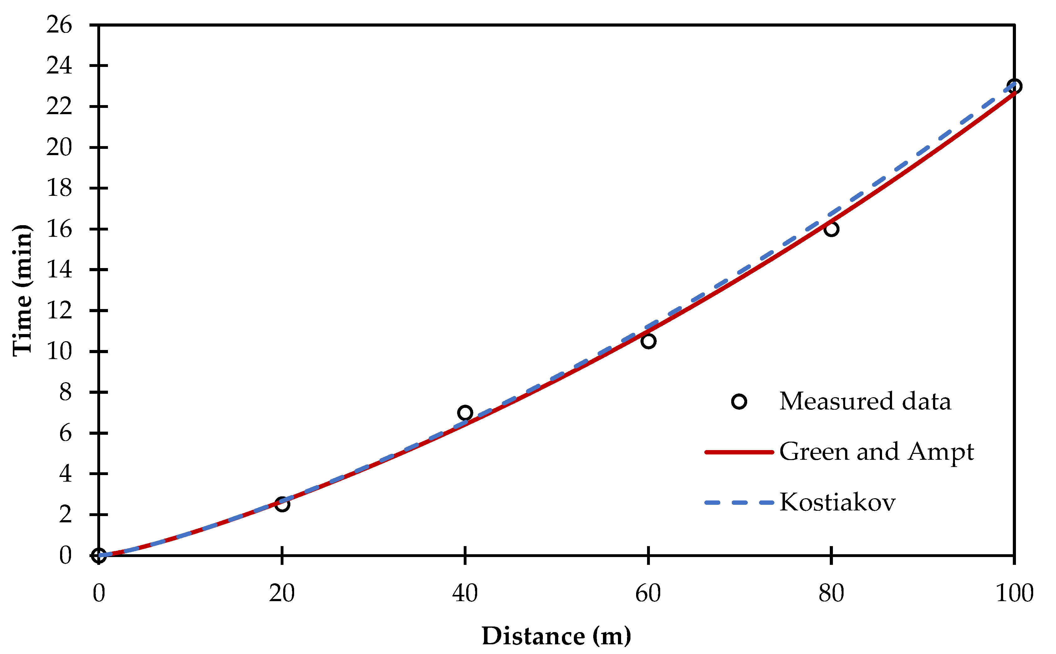
Experimental data were taken from the advance phase of an irrigation test in a closed border with loam soil [17]. In this test, the length of the border was L = 100 m, the discharge during irrigation was q₀ = 0.0032 m³/s/m, the topographic slope was J₀ = 0.002 m/m, the dimensionless parameter was β = 0, d = 1 of the hydraulic resistance law, and the initial and saturation moisture contents were θ_o = 0.2749 cm³/cm³ and θ_s = 0.4865 cm³/cm³, respectively. The values for the empirical parameters of the Kostiakov equation κ = 0.0008 m/s^α and α = 0.5271 were obtained with the Levenberg–Marquardt algorithm [26], while for the Green and Ampt equation, the parameters obtained were K_s = 1.54 cm/h and h_f = 38.00 cm.

Figure 2 shows the advance curve obtained: (a) with the measurement data in the field, (b) with the Kostiakov infiltration equation, by optimizing the parameters, and (c) by applying the Green and Ampt equation. The R² coefficients for each model were 0.998 and 0.9978, respectively. The RMSE value is a statistical estimator that serves to verify the accuracy of the model presented [4]. For the Kostiakov equation, RMSE = 1.94 m in the advance phase, while for the Green and Ampt equation, RMSE = 1.52 m.

In order to optimize the missing parameters in the infiltration functions and to retain similarity in the infiltration functions, a normal depth of h_o = 2 cm was considered in both cases.

3.2. Second Irrigation

There is a process of redistribution of moisture content due to the processes of evaporation and transpiration of the crop that depends on the phenological stage in which it is found, as well as the climate factors that prevail in the area. With the latter, it is possible to calculate the net irrigation depth necessary for optimal crop development [27]. In order to verify the coupling of the infiltration equations used, a second irrigation simulation was carried out, taking into account that the initial moisture content is different due to the redistribution, evaporation, and transpiration processes that occur from the first irrigation. Therefore, it is necessary to calculate the net irrigation depth needed to satisfy the needs of the crop in a particular phenological stage, and it is necessary to modify the input discharge in the plot to obtain an efficient distribution of the required irrigation depth along the border or furrow.

These calculations were made with an initial moisture content of θ_o = 0.1285 cm³/cm³ and, according to Equation (22), the determination of ${\ell }_{\mathrm{n}}$ = 12 cm requires the optimal irrigation flow in the border entry of q_opt = 0.001511 m³/s/m. Figure 3 shows the differences between the advanced curves observed for the two infiltration functions used for this test. This discrepancy is due to the fact that the Kostiakov equation is not a function of physical parameters from soil as initial moisture content, contrary to the Green and Ampt equation, which take this into account for the first irrigation.

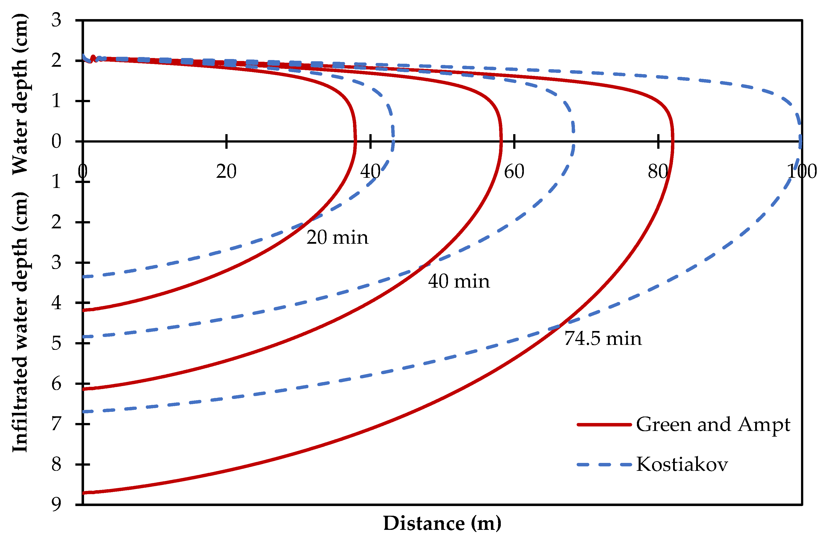
Figure 4 shows the water-depth profiles and infiltrations at different times along the border for both infiltration functions. The water-depth profile shows that, for both infiltration equations, a normal depth value of h_o = 2 cm is obtained, which show us a similarity between the two models. In addition, we obtained a faster wave front when the Kostiakov equation was used. This causes a moisture content deficit in the soil profile because the faster wave front is reduced when the water’s contact with the soil is lessened. Instead, the Green and Ampt equation is referred to as a two-parameter model because it includes two important hydraulic parameters. Sorptivity is the first of these two hydraulic parameters, using the initial and soil moisture at saturation, as well as the water’s depth. Hydraulic conductivity at saturation is the other parameter [28,29]. With this equation, the advance process is slower and favors a better redistribution of the moisture content in the soil profile.

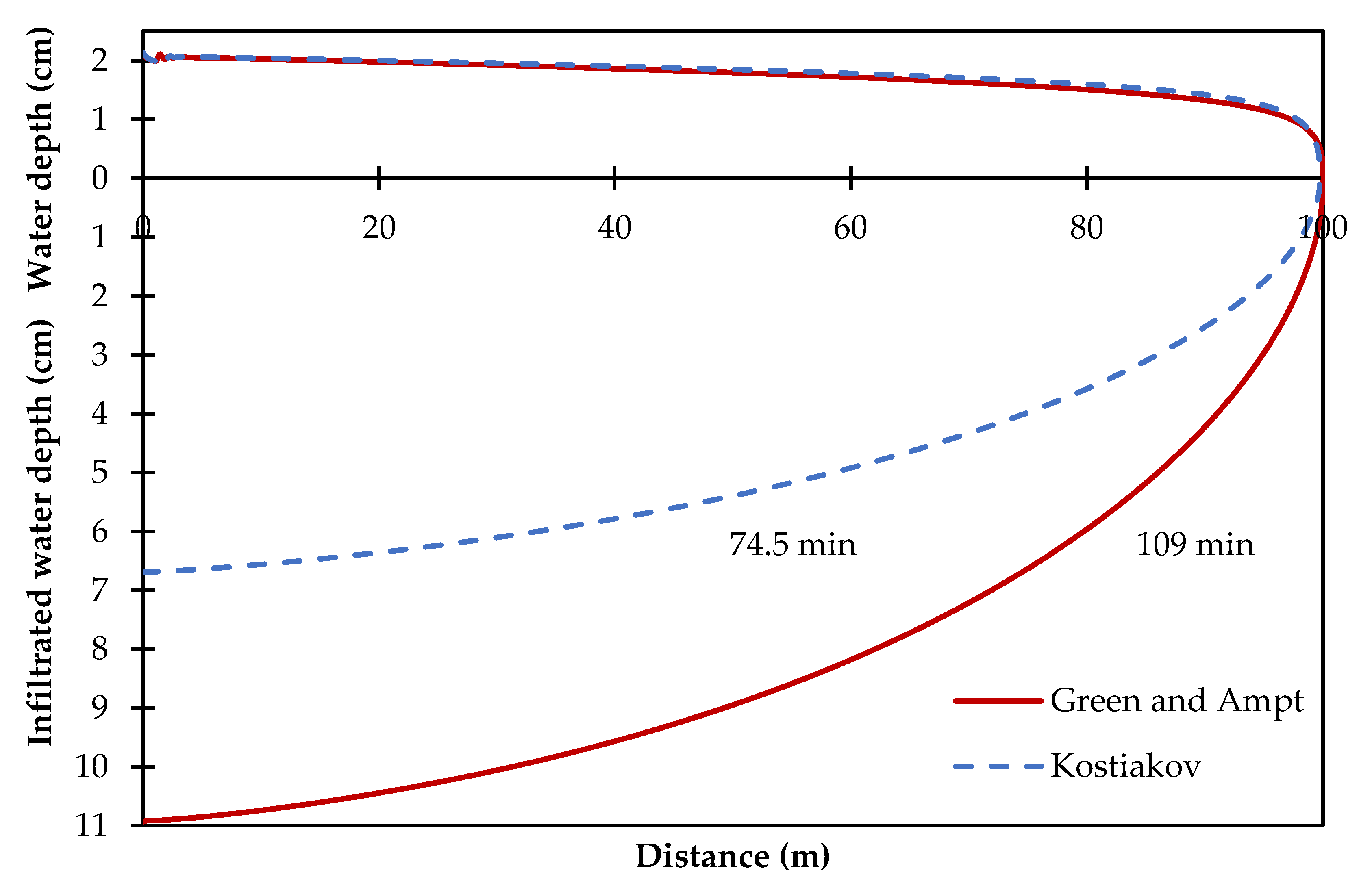
When the wave front of both functions reaches the final part of the border, the infiltration profiles are completely different (Figure 5) due to the physical parameters of the soil that changed with respect to the first irrigation. It is also observed that the wave fronts reach the end of the border at different times, caused by soil moisture that modifies the speed of the wave-front profile, which generates a longer contact time of the water with the soil, and it obtains higher infiltration. Carrying out an analysis of the input discharge and the irrigation time, the average infiltrated depths in the soil profile were 6.75 cm for Kostiakov, and 9.88 cm for Green and Ampt. This result leads to a moisture deficit for the established crop of 3.13 cm, which is equivalent to 31.65% in relation to the crop water required if the Kostiakov equation is used to apply the second irrigation.

3.3. Infiltrated Water Depth with Variable Discharge

One option for using the Kostiakov equation for gravity irrigation design is to fit this function to the simulation obtained with the Green and Ampt equation. For comparison,

Table 1. Mean parameters of the Green and Ampt equation for a loam soil used for surface irrigation design.

Soil	θo (cm3/cm3)	θs (cm3/cm3)	hf (cm)	Ks (cm/h)
Silty loam	0.17	0.55	30.00	1.00

shows the average values of the Green and Ampt equation parameters for a silty loam soil [16]. Knowing these values, which are a function of soil texture, allows for the calculation of the optimal discharge for a specific soil texture, which is directly related to the crop water required by the crop and the length of the border.

Considering L = 100 m, J₀ = 0.002 m/m, β = 0, and d = 1, from Equation (2), the optimal irrigation flow is q_opt = 0.001146 m³/s/m for ${\ell }_{\mathrm{n}}$ = 8 cm. In Figure 6, the advanced curve fitting is shown for the two models—the Green model, and the Ampt and Kostiakov model—which results in κ = 0.00067 m/s^α and α = 0.544 using the Levenberg–Marquardt optimization algorithm.

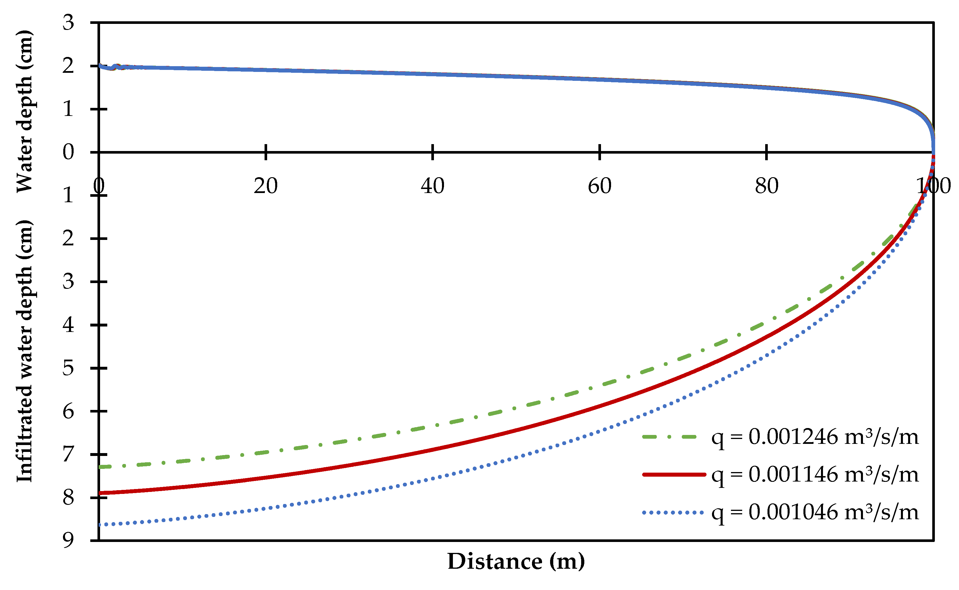
Figure 7 presents a variation of ±0.0001 m³/s/m from the optimal irrigation flow using the Kostiakov infiltration equation with the optimized parameters, where the infiltrated water depth and the irrigation time were modified. The value of infiltrated average depth in the soil profile using q = 0.001046 m³/s/m was 5.96 cm, with a q_opt of 7.56 cm, which produced a moisture deficit of 1.60 cm (31.65 %). On the other hand, if q = 0.001246 m³/s/m, the infiltrated average depth was 9.68 cm, which produced a moisture excess of 2.12 cm (28%) for crops. These results show that it is possible to use this equation for a first design [15,30]. However, if the Green and Ampt model was already calculated, it is better to use it, because the minimal variations in the input parameters generate a broad value in the results that is derived in water excesses or moisture deficits [3,16].

4. Discussion

With the study of the advance phase of an irrigation test, it is possible to estimate the parameters of the Kostiakov equation and the Green and Ampt equation. The empirical Kostiakov equation is theoretically influenced by the physical characteristics of the soil, moisture contents, and the measurement techniques of the irrigation test. In addition, the Kostiakov model should be used for times t < t_max where t_max = (k_b/k_s)^1/(1−b), where k_b is the basic infiltration and b is a shape parameter [15]. However, this only occurs for a specific irrigation event, since the parameters are adjusted to an initial irrigation test that does not represent the subsequent irrigations due to the change, mainly, of the initial moisture. On the other hand, the parameters of the Green and Ampt equation are based on the physical characteristics of the soil. Therefore, it is possible to adequately represent the subsequent irrigations to determine what really happens in the advance/infiltration process of the gravity irrigation.

It is important to determine the crop water requirements and the appropriate moments of their application to cover the irrigation sheet needs of the crops established in the plots, because the variation of the moisture content in the soil is a factor that limits the development and yield of the crops in agriculture [31]. The initial moisture content determines the irrigation time, optimal irrigation flow, and irrigation sheet that should be supplied in the plot to bring the soil to field capacity [25]. The CROPWAT software [32] can be used as an alternative to calculate the crops’ needs from climatic data of the area and the crop phenological stage [33], if the latter cannot be provided by weather stations near the study area.

The input discharge applied in surface irrigation considerably modifies the infiltrated depth and the irrigation time, regardless of the infiltration function used. In this work, an analysis of the inflows in the plot considering the Kostiakov infiltration equation was performed. This same process occurs with the Green and Ampt equation, since by increasing the optimal irrigation flow, a higher speed of the advancing wave is obtained, which causes a shorter contact time of the water with the soil and generates a decrease in the infiltrated depth [3]. However, in clay soils where K_s is very low, the irrigation time increases, and consequently, the input discharge must be lower [25], and the interpretations of the parameters required for the Kostiakov equation are empirical and do not represent what happens in an irrigation event in a particular soil.

The coupling of the hydrodynamic wave model shown here demonstrates that, by using the Green and Ampt equation, it becomes a robust and efficient model for designing subsequent irrigations. However, by using the Kostiakov equation, it becomes a representative model of an empirical irrigation test. Software such as WinSRFR [12], SIRMOD [13], and SISCO [14], which in addition to the Kostiakov equation, use the empirical Kostiakov–Lewis equation, is, therefore, deficient for the design of surface irrigation in an optimal and opportune manner. There is a need for prior-irrigation measurements, calculations, or estimations of the important hydraulic parameters of the soil involved in the infiltration process [34].

5. Conclusions

Using the numerical coupling of the Saint-Venant equations with the empirical Kostiakov equation, it was shown that this only represents a specific irrigation event, precisely the irrigation test with which the optimization of the function parameters is carried out. However, by coupling the Green and Ampt equation with the optimization of the parameters of K_s and h_f from the same irrigation test, it is possible to model the subsequent irrigations, because the latter infiltration function makes use of the physical parameters of the soil in order to observe the infiltration process in the surface irrigation in detail.

In addition, it was shown that by varying the inflows in the plot, the infiltrated water depths are modified, causing deficits or excesses of water required by the crop established in the border, without taking into account the infiltration equation used. As a result, it is considered important to efficiently calculate the optimal irrigation flow, which depends on the border length, the net irrigation depth to be applied, the moisture content, and the parameters of the infiltration equation to be used. These results allow us to recommend the Green and Ampt equation as the best equation for the design and modeling of surface irrigation. The Green and Ampt equation is based on the physical parameters of the soil, and if in some cases all the information required by the model is not available, specialized bibliography can be consulted, in which average values for efficient design that are based on soil texture are recommended [16].

References

- Akbari, M.; Gheysari, M.; Mostafazadeh-Fard, B.; Shayannejad, M. Surface Irrigation Simulation-Optimization Model Based on Meta-Heuristic Algorithms. Agric. Water Manag. 2018, 201, 46–57. [Google Scholar] [CrossRef]
- Khasraghi, M.M.; Sefidkouhi, M.A.G.; Valipour, M. Simulation of Open- and Closed-End Border Irrigation Systems Using SIRMOD. Arch. Agron. Soil Sci. 2015, 61, 929–941. [Google Scholar] [CrossRef]
- Fuentes, S.; Fuentes, C.; Saucedo, H.; Chávez, C. Border Irrigation Modeling with the Barré de Saint-Venant and Green and Ampt Equations. Mathematics 2022, 10, 1039. [Google Scholar] [CrossRef]
- Golestani Kermani, S.; Sayari, S.; Kisi, O.; Zounemat-Kermani, M. Comparing Data Driven Models versus Numerical Models in Simulation of Waterfront Advance in Furrow Irrigation. Irrig. Sci. 2019, 37, 547–560. [Google Scholar] [CrossRef]
- Chávez, C.; Fuentes, C. Design and Evaluation of Surface Irrigation Systems Applying an Analytical Formula in the Irrigation District 085, La Begoña, Mexico. Agric. Water Manag. 2019, 221, 279–285. [Google Scholar] [CrossRef]
- Ebrahimian, H.; Liaghat, A. Field Evaluation of Various Mathematical Models for Furrow and Border Irrigation Systems. Soil Water Res. 2011, 6, 91–101. [Google Scholar] [CrossRef] [Green Version]
- Adamala, S.; Raghuwanshi, N.S.; Mishra, A. Development of Surface Irrigation Systems Design and Evaluation Software (SIDES). Comput. Electron. Agric. 2014, 100, 100–109. [Google Scholar] [CrossRef]
- Walker, W.R.; Humpherys, A.S. Kinematic-Wave Furrow Irrigation Model. J. Irrig. Drain. Eng. 1983, 109, 377–392. [Google Scholar] [CrossRef]
- Gonzalez, C.J.M.; Muñoz, H.B.; Acosta, H.R.; Mailhol, J.C. Kinematic Wave Model Adapted to Irrigation with Closed-End Furrows. Agrociencia 2006, 40, 731–740. [Google Scholar]
- Strelkoff, T.; Katopodes, N.D. Border-Irrigation Hydraulics with Zero Inertia. J. Irrig. Drain. Div. 1977, 103, 325–342. [Google Scholar] [CrossRef]
- Elliott, R.L.; Walker, W.R.; Skogerboe, G.V. Zero-Inertia Modeling of Furrow Irrigation Advance. J. Irrig. Drain. Div. 1982, 108, 179–195. [Google Scholar] [CrossRef]
- Bautista, E.; Schlegel, J.L.; Clemmens, A.J. The SRFR 5 Modeling System for Surface Irrigation. J. Irrig. Drain. Eng. 2016, 142, 04015038. [Google Scholar] [CrossRef]
- Walker, W.R. SIRMOD III: Surface Irrigation Simulation, Evaluation and Design-Guide and Technical Documentation; Utah State University: Logan, UT, USA, 2003. [Google Scholar]
- Gillies, M.H.; Smith, R.J. SISCO: Surface Irrigation Simulation, Calibration and Optimisation. Irrig. Sci. 2015, 33, 339–355. [Google Scholar] [CrossRef]
- Singh, V.; Bhallamudi, S.M. Complete Hydrodynamic Border-Strip Irrigation Model. J. Irrig. Drain. Eng. 1996, 122, 189–197. [Google Scholar] [CrossRef]
- Saucedo, H.; Zavala, M.; Fuentes, C. Border irrigation design with the Saint-Venant and Green & Ampt equations. Water Technol. Sci. 2015, 6, 103–112. [Google Scholar]
- Saucedo, H.; Fuentes, C.; Zavala, M. The Saint-Venant and Richards Equation System in Surface Irrigation: (2) Numerical Coupling for the Advance Phase in Border Irrigation. Ing. Hidraul. Mex. 2005, 20, 109–119. [Google Scholar]
- Kostiakov, A.N. On the Dynamics of the Coefficient of Water Percolation in Soils and the Necessity of Studying It from the Dynamic Point of View for the Purposes of Amelioration. Trans. Sixth Comm. Int. Soc. Soil Sci. 1932, 1, 7–21. [Google Scholar]
- Green, W.H.; Ampt, G.A. Studies on Soil Physics, I: The Flow of Air and Water through Soils. J. Agric. Sci. 1911, 4, 1–24. [Google Scholar]
- Walker, W.R.; Skogerboe, G.V. Surface Irrigation. Theory and Practice; Prentice-Hall, Inc.: Englewood Cliffs, NJ, USA, 1987. [Google Scholar]
- Fuentes, S.; Chávez, C. Modeling of Border Irrigation in Soils with the Presence of a Shallow Water Table. I: The Advance Phase. Agriculture 2022, 12, 426. [Google Scholar] [CrossRef]
- Strelkoff, T. EQSWP: Extended Unsteady-Flow Double-Sweep Equation Solver. J. Hydraul. Eng. 1992, 118, 735–742. [Google Scholar] [CrossRef]
- Liu, K.; Xiong, Y.; Xu, X.; Huang, Q.; Huo, Z.; Huang, G. Modified Model for Simulating Water Flow in Furrow Irrigation. J. Irrig. Drain. Eng. 2020, 146, 06020002. [Google Scholar] [CrossRef]
- Tabuada, M.A.; Rego, Z.J.C.; Vachaud, G.; Pereira, L.S. Modelling of Furrow Irrigation. Advance with Two-Dimensional Infiltration. Agric. Water Manag. 1995, 28, 201–221. [Google Scholar] [CrossRef]
- Fuentes, C.; Chávez, C. Analytic Representation of the Optimal Flow for Gravity Irrigation. Water 2020, 12, 2710. [Google Scholar] [CrossRef]
- Moré, J.J. The Levenberg-Marquardt Algorithm: Implementation and Theory. In Numerical Analysis; Watson, G.A., Ed.; Springer: Berlin/Heidelberg, Germany, 1978; pp. 105–116. [Google Scholar]
- Allen, R.G.; Pereira, L.S.; Raes, D.; Smith, M. Crop Evapotranspiration-Guidelines for Computing Crop Water Requirements; FAO Irrigation and Drainage Paper 56; FAO: Rome, Italy, 1998; Volume 300, p. D05109. [Google Scholar]
- Angelaki, A.; Sihag, P.; Sakellariou-Makrantonaki, M.; Tzimopoulos, C. The Effect of Sorptivity on Cumulative Infiltration. Water Supply 2021, 21, 606–614. [Google Scholar] [CrossRef]
- Stewart, R.D.; Rupp, D.E.; Najm, M.R.A.; Selker, J.S. Modeling Effect of Initial Soil Moisture on Sorptivity and Infiltration: Effect of Initial Soil Moisture on Sorptivity & Infiltration. Water Resour. Res. 2013, 49, 7037–7047. [Google Scholar] [CrossRef]
- Shayannejad, M.; Ghobadi, M.; Ostad-Ali-Askari, K. Modeling of Surface Flow and Infiltration During Surface Irrigation Advance Based on Numerical Solution of Saint–Venant Equations Using Preissmann’s Scheme. Pure Appl. Geophys. 2022, 179, 1103–1113. [Google Scholar] [CrossRef]
- Du, K.; Qiao, Y.; Zhang, Q.; Li, F.; Li, Q.; Liu, S.; Tian, C. Modeling Soil Water Content and Crop-Growth Metrics in a Wheat Field in the North China Plain Using RZWQM2. Agronomy 2021, 11, 1245. [Google Scholar] [CrossRef]
- Spiliotopoulos; Loukas Hybrid Methodology for the Estimation of Crop Coefficients Based on Satellite Imagery and Ground-Based Measurements. Water 2019, 11, 1364. [CrossRef] [Green Version]
- Muñoz, G.; Grieser, J. Climwat 2.0 for CROPWAT; Water Resources, Development and Management Service: Rome, Italy, 2006; pp. 1–5. [Google Scholar]
- Yusuf, K.O.; Ejieji, C.J.; Baiyeri, M.R. Determination of Sorptivity, Infiltration Rate and Hydraulic Conductivity of Soil Using a Tension Infiltrometer. Wildl. Environ. 2018, 10, 99–108. [Google Scholar]
Figure 1.
Individual cell scheme at two different times.
Figure 2.
Advance curve for measured data from the first irrigation test.
Figure 3.
Advanced curves for the two infiltration equations for a second irrigation application.
Figure 4.
Variation of infiltration at different times.
Figure 5.
Water depth and infiltration at the border end.
Figure 6.
Parameter optimization of the Kostiakov infiltration equation from the Green and Ampt advanced curve.
Figure 7.
Variation of the infiltration during the advance phase for three different inflows.