
Understanding Coastal Resilience of the Belgian West Coast


1
Flanders Hydraulics Research, Berchemlei 115, 2140 Antwerpen, Belgium
2
Antea Group Belgium, Roderveldlaan 1, 2600 Antwerpen, Belgium
3
Hydrology and Hydraulic Engineering, Vrije Universiteit Brussel, 1050 Brussel, Belgium
4
Fides Engineering, Unitaslaan 11, 2100 Antwerpen, Belgium
*
Author to whom correspondence should be addressed.
Water 2022, 14(13), 2104; https://doi.org/10.3390/w14132104
Submission received: 17 March 2022
/
Revised: 20 June 2022
/
Accepted: 23 June 2022
/
Published: 30 June 2022
(This article belongs to the Special Issue Advances in Coastal Hydrodynamics and Morphodynamics)
Abstract
:Topobathymetric monitoring carried out in the past 30 years revealed that the amount of sand in the active zone of the Belgian West Coast increased substantially. Correcting for sand works carried out, the rate of natural feeding of the area was estimated to be 10 mm/year, which is significantly more than the local sea level rise rate of 2 to 3 mm/year. One concludes that this coastal zone, with a length of ca. 16 km, has shown a natural resilience against sea level rise. The question remains which processes govern this behavior and where natural input of sand to the system occurs. Using available coastal monitoring data for the Belgian coast, as well as a state-of-the-art sand transport model, revealed that different processes drive a cross-shore natural feeding from offshore to the coastline. The spatial distribution of this cross-shore natural feeding is determined by the existence of a gully-sand bank system. The outcome of this research was a conceptual model for the large-scale sand exchange in the study area which is implemented in an 1D coastline model. The most important element in these models was the cross-shore natural feeding of the active zone via a shoreface connected ridge amounting to 95,000 m3/year in the period 2000–2020.
1. Introduction
1.1. The Belgian West Coast
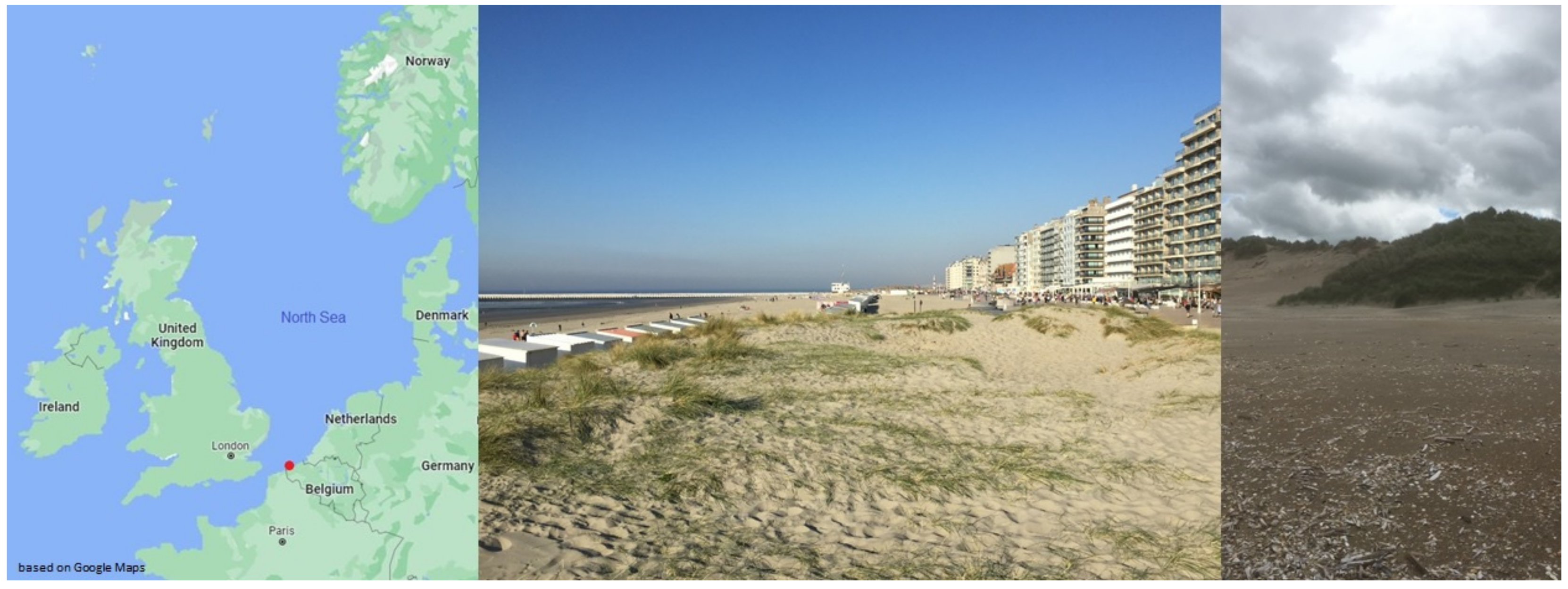
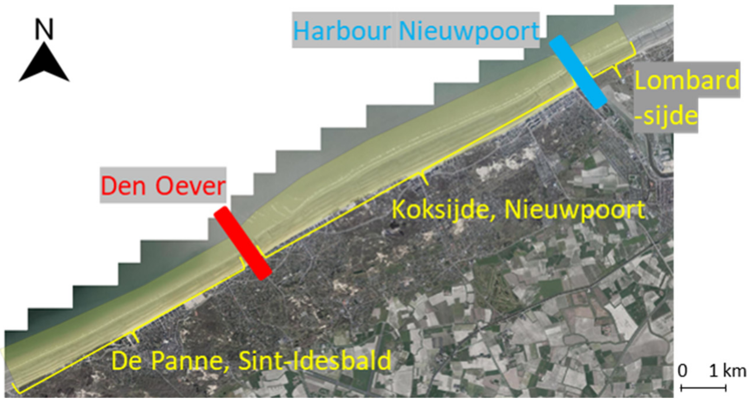
The Belgian West Coast is situated in the southern part of the North Sea at the border with France (Figure 1). It is a sandy coast with a length of ca. 16 km. Natural stretches with high dunes alternate with coastal towns where low dunes can be present. This coast is part of the sandy coast stretching from the north of France (Dover Strait) until the northern tip of Denmark (Jutland). The Southern North Sea is a shallow sea that has been formed by sea level rise after the last ice age. Mean depth of the Belgian part of the North Sea is around 40 m 50 km offshore. The sea bottom is undulating due to the presence of large scale bedforms: sandbanks and gullies.
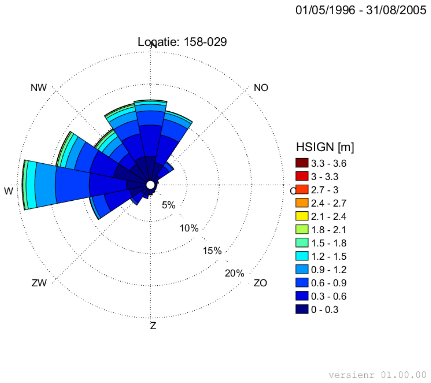
The mean tidal range in the study area is 4 m. High tide and low tide alternate twice a day (semidiurnal tide). Wide intertidal beaches are present with a mild slope between 1/50 and 1/100. An average significant wave height in front of the coast is 60 cm and 10% of the time 2 m is exceeded. Locally generated wind waves are dominant compared to swell propagated from large distance. The reason for this is the sheltering that is provided by Great Britain (United Kingdom and Ireland) from the Atlantic. Winds most frequently come from the southwest, but can come from other directions as well. Average wind speed is 8 m/s.
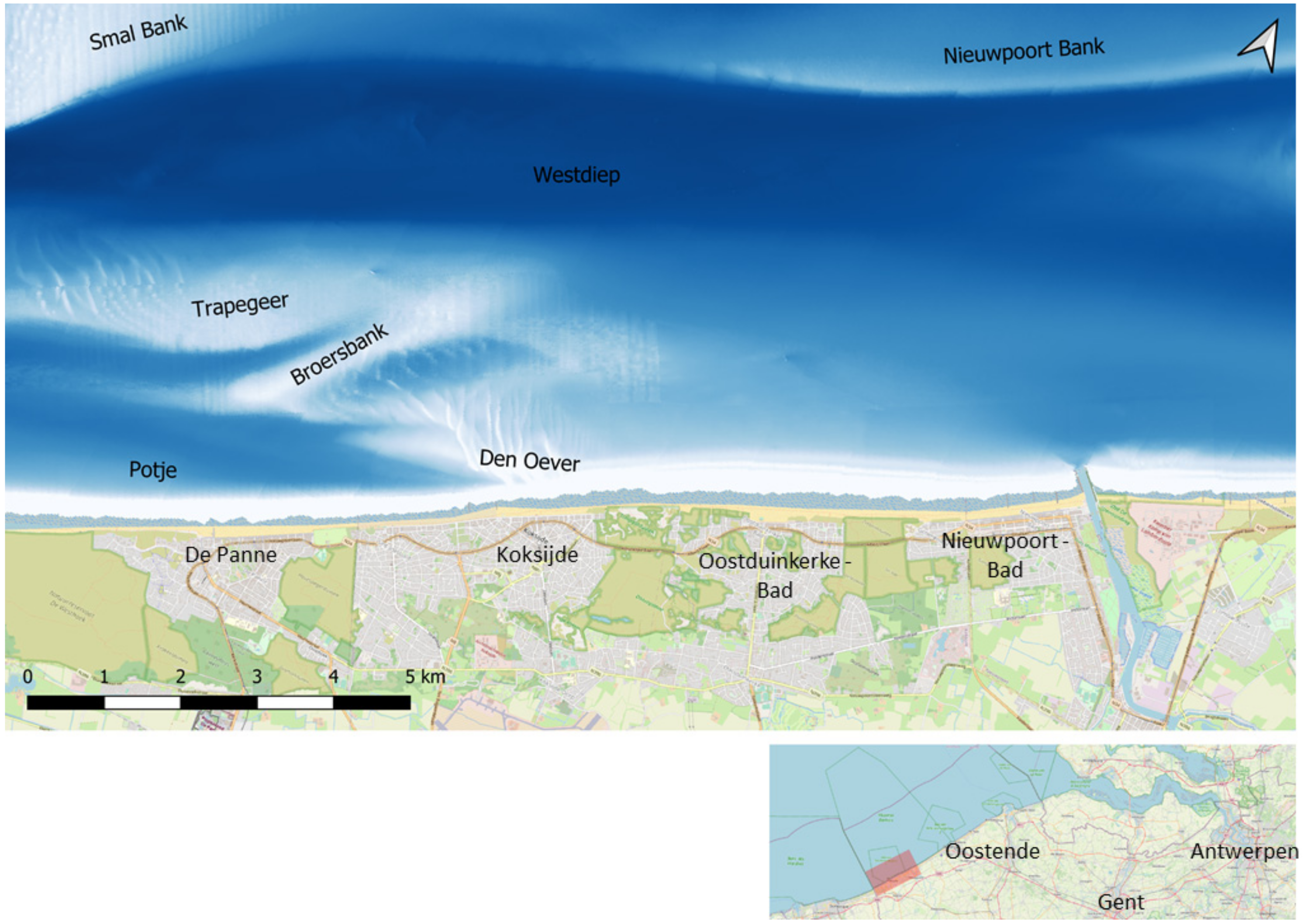
Close to the coastline the sand banks and gullies interact with the beach morphology (Figure 2). In the west of the study area the coastline is influenced by a gully (Potje) which causes rather steep cross shore slopes. At the end of this gully a very shallow area is situated (Broersbank, Trapegeerbank, Den Oever). East of this shallow area the beaches have mild slopes. In the east of the study area the harbour of Nieuwpoort with its navigation channel is a sink for the alongshore sediment transport.
1.2. New Research
Why have we carried out this research? There are two reasons for this.
Firstly, we wanted to explain our observations of resilience to sea level rise of this coast. In previous research on the Belgian coast [1], we compared the sea level rise in the past 30 years with the change in sand volume of the beaches, active shorefaces and dunes for the Belgian West Coast. The result was a much larger growth rate of 10 mm/year compared with the sea level rise of 2 to 3 mm/year. So, there must be a natural feeding into this zone. However, we wanted answers to the following questions: how much of the feeding comes from along shore, how much comes from cross-shore, and is this resilience uniform over the area considered?
A second goal was to establish a morphological model on the time scale of decennia to centuries. Such models can be tools for predicting morphological effects of sea level rise, as well as effects of large infrastructure works. The model should be able to predict, for example, the retreat of a coastline, according to the Bruun rule, but also the progradation of a coastline in cases where natural feeding is dominating the Bruun rule effect [2]. How did we approach this? We approached it by establishing an 1D coastline model. This means that we adopted the concept of equilibrium profile and that the behavior of the coastline was described by Equation (1) from [3].
where cp = coastline retreat rate [m/y]; h* = active height of the profile [m]; ∂MSL/∂t = sea level rise rate [m/j]; L* = width of the active zone [m]; qx,sea = cross-shore feeding of the active zone from the neighbouring sea bottom [m3/m/y]; qx,dune = flux towards the dunes [m3/m/y]; Qy = littoral drift [m3/y]; and s = nourishment intensity [m3/m/y].
The position of the coastline on the left side of the equation multiplied with the active height of the profile is described by a summation of influences by five different processes on the right side of the equation. The first term corresponds to the Bruun rule. In literature, some authors give objections to Bruun rule application [4,5]. Although Bruun rule is a simplification of reality, it has been applied often (e.g., [6,7]). The second term refers to cross-shore feeding to the active zone from the sea bottom. The third term represents aeolian loss to the dunes. The fourth term refers to the gradients in littoral drift. Finally, the fifth and last term accounts for human interventions, nourishments or sand extractions.
Previous morphological research on the Belgian coast has identified morphological trends based on yearly topobathymetric monitoring [8] and on an analysis of historical maps [9]. A process-based model linking morphological changes to tides and waves as driving forces, named Scaldis-Coast, has been set up in the littoral zone, on a time scale of years for previous research [10]. The novelty of the new research was to set up a model on a time scale of decades to centuries. The 1D coastline model approach was chosen to simulate coastal morphological change on a decadal time scale as well as to obtain stability of the coastal profile. The 1D model is not able to capture all complex processes in the model domain. It is a simplification that permits the performing of long-term modelling. Nonetheless, the output from the state-of-the-art 2DH model, Scaldis-Coast, as input/calibration data was used for the 1D coastline model. 2DH models often have difficulties in simulating long-term behaviour of the coastline, because of unrealistic cross-shore evolution building up in time, which is the case for the Scaldis-Coast. In this study, the approach was to combine advantages from 2DH modelling (simulating spatial distribution of tidal and wave driven sediment fluxes) and 1D coastline modelling (stability of the cross-shore profile). Combining advantages of both modelling approaches has been followed by others for other coastal regions, e.g., for describing interaction of tidal sand banks with the coastline [11] and for the evolution of the Sand Motor in the Netherlands [12].
The principal result of this research was a conceptual model for the large-scale sand exchange in the study area which was implemented in a 1D coastline model. The most important element in these models was the cross-shore natural feeding of the active zone via a shoreface connected ridge amounting to 95,000 m3/year in the period 2000–2020.
The novelty of this work is that it explains that the Belgian West Coast shows natural resilience to sea level rise because of the presence of the shoreface-connected ridge and gully system present at this coast. The work was based on an extensive morphological data set and 2DH modelling. This mechanism generated a natural feeding of this coast. In general, one expects a retreat of a coastline due to sea level rise, but in this case the opposite was observed. This is important for coastal protection purposes. To the authors’ knowledge, this phenomenon has never before been described in literature for the Belgian coast. Nearshore and coastal engineering of installations at the Belgian west coast should consider the natural morphological interaction between the ridge-gully system and the beaches to optimize environmental impacts. For instance, such considerations could be relevant to determine cable landing sites. In practice, however, due to Natura 2000 restrictions few other installations can be built in this coastal zone, so a more detailed discussion on this point is excluded from this paper.
2. Materials and Methods
2.1. Materials
Digital elevation models, wave and tidal data, grain size measurements and descriptions of human interventions, for the study area, for the twenty-year period considered, from 2000 to 2020, were provided by the managing coastal authority from the Flemish regional government. For non-commercial research purposes all these data are freely available on demand. Digital elevation models are established by combining airborne Light Detection and Ranging (LIDAR) surveying for the dry part of the profile, and cross-shore profiles for every ca. 100 m are provided by single beam echo-sounding from a sailing vessel [13]. Wave and tidal data are gathered by the Flemish government at fixed locations that form the hydrometeorology monitoring network named “Vlaamse Banken” [14]. In addition, campaigns at other locations have been carried out by Flemish Hydrography. Grain size measurements were carried out, mainly on the beaches. The large nourishments carried out by the Flemish regional government are well documented for the period considered. Little information was available for local sand works that were carried out by coastal communities in coastal town centers, such as reprofiling the upper beach to create a horizontal berm and bringing back aeolian deposits on the dike to the beach. Nevertheless, these works were less important, due to their small size and local impact, so that their impacts were neglected on the scale of the Belgian West Coast, as a whole.
For the 1D coastline model, software Unibest was used [15], which is licensed software from Deltares (Delft, The Netherlands). Profiles were taken from a published data-set with 100 m spacing [13], which was derived from the ca. yearly topobathymetric monitoring data. In total, 160 profiles described the study area. For 14 moments in time, combined topographic and bathymetric survey results were available.
2.2. Methods
2.2.1. Morphological Analysis
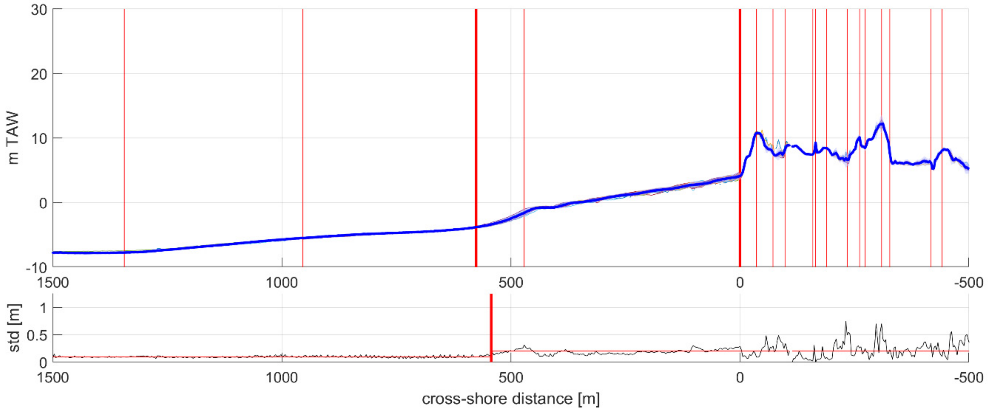
The first step was to analyze the morpho-dynamics in profiles to determine the seaward boundary and the landward boundary of the active beach and shoreface zone. As stated in [16], the most reliable method (if enough data are available) for estimating the depth of closure is to perform a morphological analysis (especially when the time scale of the available data corresponds with the time period of the study). By investigating the standard deviation in the profile, as well as the changepoints in the slope of the profile, the depth of closure at the seaward side and the dune foot at the landward side were determined. In Figure 3, this procedure is illustrated: in the upper panel, the location of the changepoints in the slope are shown, and in the lower panel the variation of the standard deviation is shown.
The next step was a volumetric analysis. The study area was subdivided into morphological uniform zones, especially delineating coastal towns and areas with natural dunes. For each zone the volumes in active beach and shoreface zone, as well as the volumes in the landward dunes, were calculated. Fixed contour lines were defined in this procedure, namely −4 m TAW as an average value for the depth of closure in the study area, and +5.9 m TAW as the boundary between the active beach and shoreface zone on the one side, and the landward dunes on the other side. These upper and lower boundaries were derived based on the results of the analysis of the profiles (cf. Section 3.1.1).
2.2.2. Modeling
A conceptual model was developed by establishing the sand balance of the study area and the sand exchanges with the surroundings. To study the littoral drift in the study area, as well as the cross-shore feeding towards the coast from the bank-gully system off-shore, a numerical model output from the operational, state-of-the-art 2DH sand transport model, Scaldis-Coast, was used, which is an implementation in the Telemac model software (www.opentelemac.org) and which includes wave and tide forcing [10].
A 1D coastline model was set up in Unibest [15]. For this 1D coastline model, we used Deltares software Unibest, which consisted of 3 modules:
- a cross-shore model (Unibest-TC),
- a littoral drift model (Unibest-LT) and
- a coastline model (Unibest-CL).
The latter 2 were combined in the package Unibest-CL+ and were used within this research.
The littoral drift model calculated the longshore transport for a given cross shore profile and a (yearly) climate of currents and waves. The (tidal) currents could be specified for a reference depth. The currents at other locations were scaled with the local depth. Different sediment transport formulations could be used to calculate the sediment transport.
The coastline model calculated the coastline changes due to longshore sediment transport gradients. Input of the coastline model were the coastline (the low water line), the transport rates obtained in the littoral drift model (for different coastline orientations), the sources (e.g., at Den Oever, where an input flux due to transport over the shallow bank was assumed) and a sink (e.g., dredging in the navigation channel of Nieuwpoort).
It should be noted that the concept of a 1D coastline model assumed a time independent shape of the cross-shore profile. The current velocities were modelled in a simplified way in Unibest (one assumed a cross-shore decrease in a profile linear with the water depth, so no dependency on the slope of the profile was taken into account). The input coastline corresponded with the measured low-water line since this line was most representative for the coastline shape. First, the longshore transport rates, as functions of the coastline orientation, were calculated for 6 cross-sections using the yearly wave climate and tidal velocities. The transport rates of the Unibest model were calibrated to the yearly sediment transport rates obtained with the 2DH model, Scaldis-Coast. Calibration was done by varying the sediment transport formulae, the coefficients in these formulae and by adjusting the wave and current conditions. The obtained tables that connected coastline orientation with sediment transport rate were input for the longshore model: gradients in sediment transport rates caused changes in coastline position and, thus, in coastline orientation, resulting in a different transport rate. This procedure was repeated for each time step for the desired modelling period. More details are given in Section 3.3.
3. Results
3.1. Morphological Analysis
3.1.1. Profiles
Table 1 presents the results of this analysis for the whole study area. One observed some variation in the study area (Table 1). For example, the width of the active zone varied between 600 m and 1000 m, the height of the active zone varied between 8 m and 13 m, and the position of the landward boundary varied between 5 m and 9 m TAW (Belgian Ordnance Datum, close to low water at spring tide).
Values obtained for the depth of closure corresponded with earlier estimates for the Belgian coast given in [17], based on the Hallermeier equation [18]. Thus, it was concluded that to determine the depth of closure for the model set-up in a pragmatic way, an average value for the study area could be used, namely −4 m TAW. In a similar way, the results for the landward boundary were compared with values reported for the dune foot position along the Belgian coast in [19] and it was concluded that an average value of +5.9 m TAW be used for the model set-up.
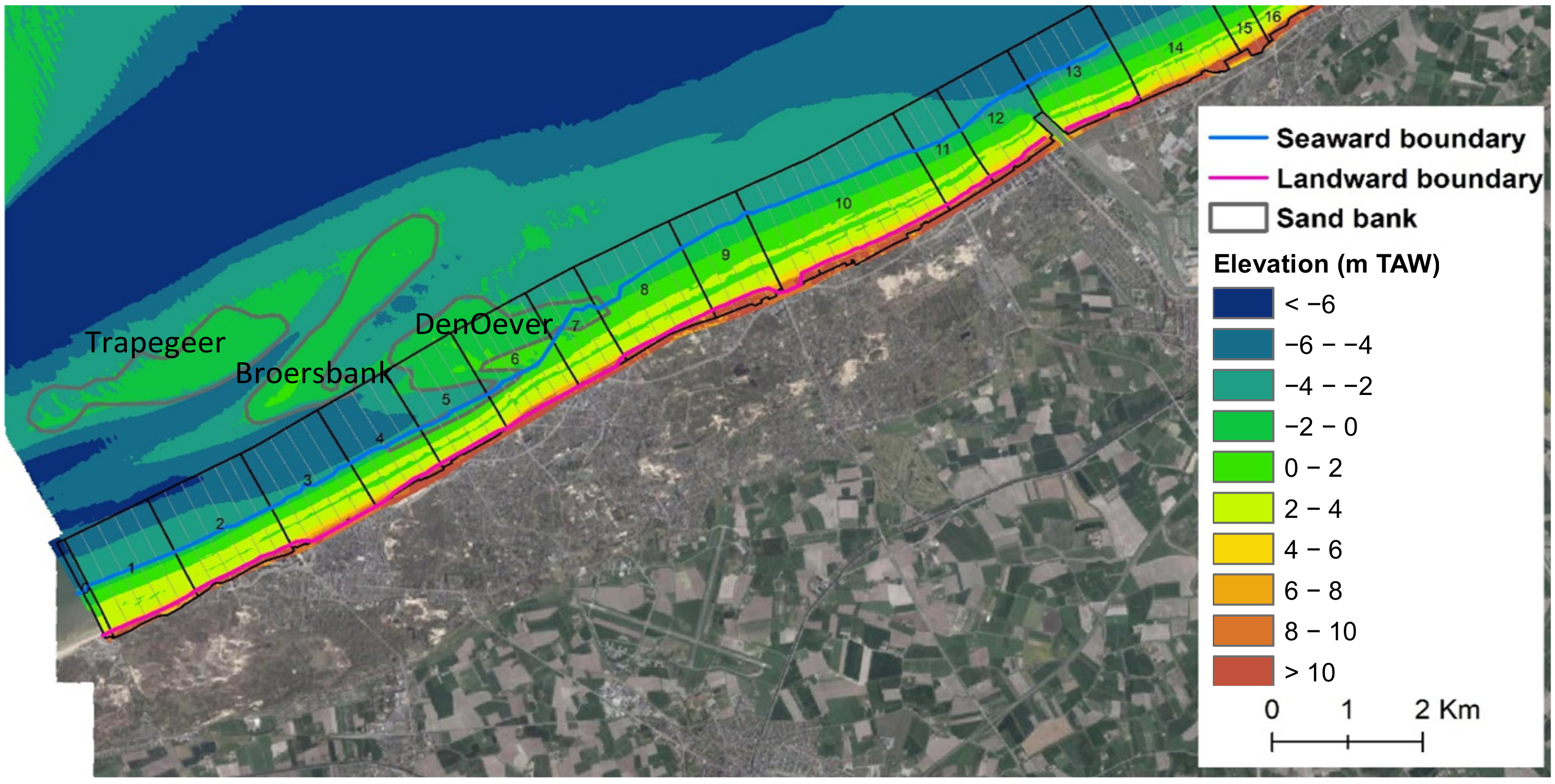
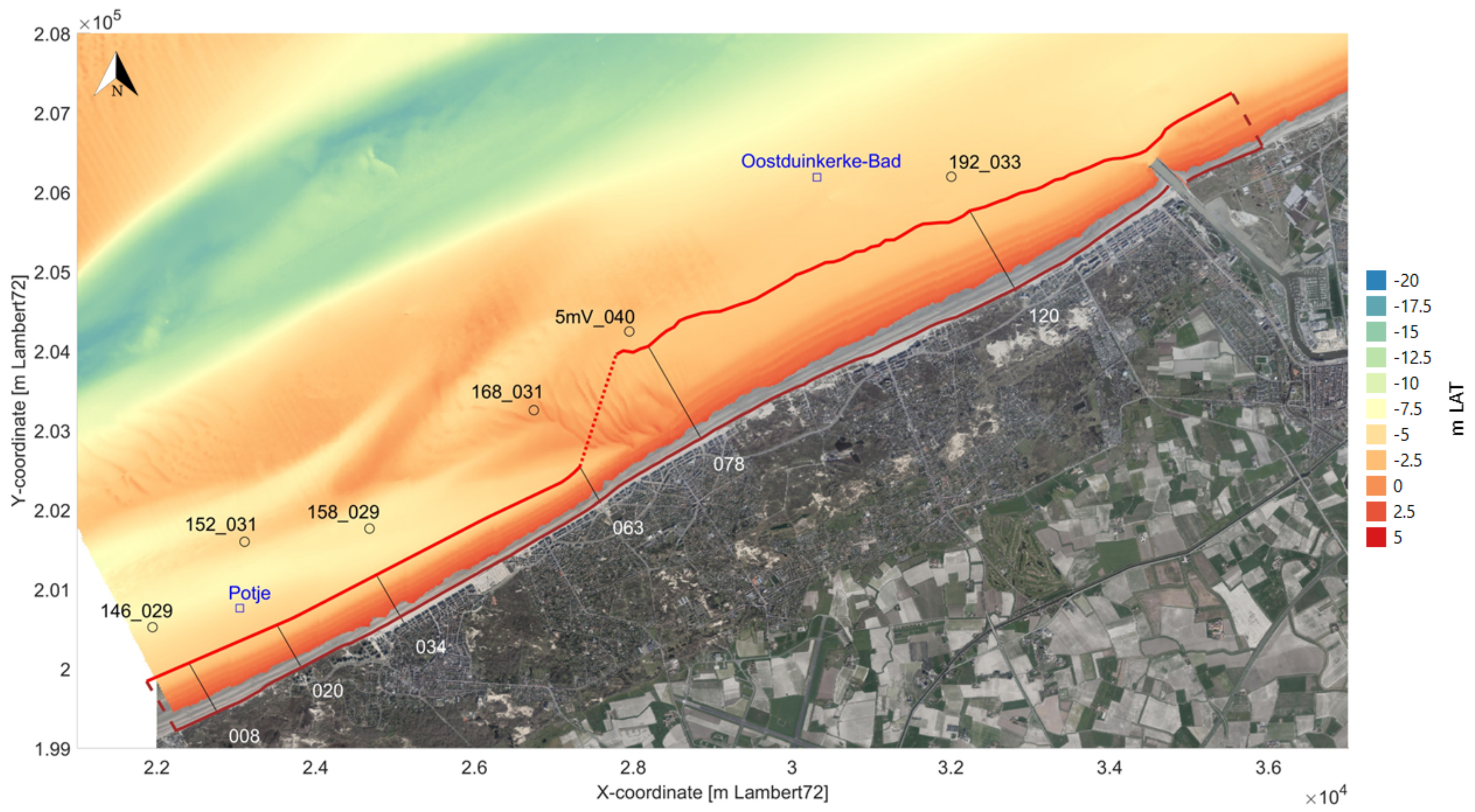
The positions of the seaward and landward boundaries are shown on Figure 4. In stretches 6 and 7, at the location Den Oever, where the shoreface connected ridge attaches to the shoreline, it was difficult to determine a seaward boundary based solely on the profile morpho-dynamics. The reason was that the top of the ridge showed morpho-dynamics of equal intensity as the beach and shoreface zone. This hurdle was overcome by using interpolation: the seaward delineation in stretch 6 was the result of a linear interpolation between the positions of the seaward boundary in the neighbouring stretches 5 and 7.
The slope of the active beach and shoreface zone varied over the study area (Figure 5). One could observe that the average slope of 1/76 was influenced by the presence of the gully-sand bank system in the study area. The slope was steeper where the gully was present, while it was milder where the sand bank was present.
3.1.2. Volumetric Analysis
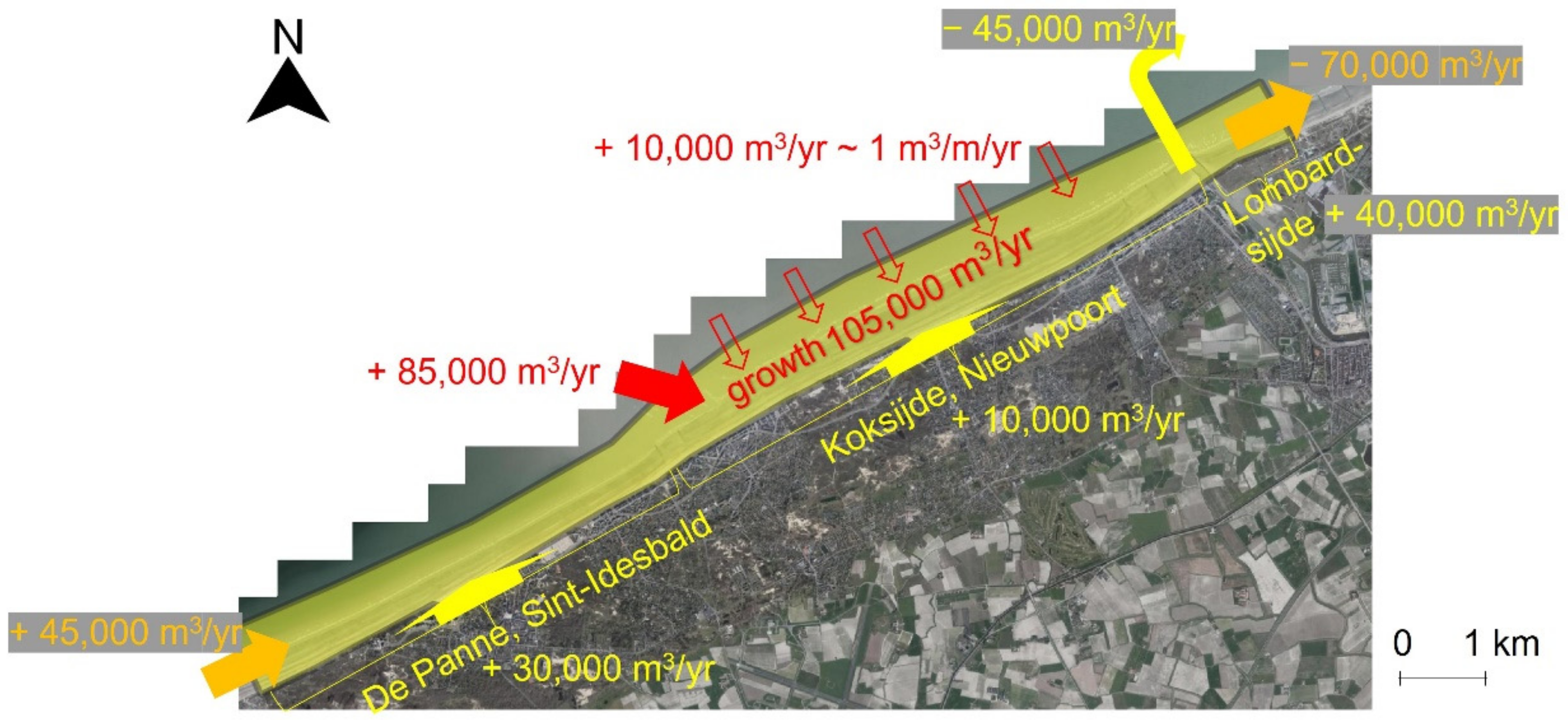
This result predominantly showed growth in available sand volume in the period from 2000 to 2020 in the 13 stretches. However, one has to also consider beach nourishments that were carried out. The nourishment intensities were very different in the different coastal towns. One could see a difference between 1 m3/m/year and 31 m3/m/year. Corrected volumetric growth was the observed growth from which nourishment volumes were subtracted. Overall, one could distinguish between three sections of the study area. In the volumetric analysis the 13 stretches were aggregated to 3 sections, namely, “De Panne−Sint-Idesbald” (stretches 1–5), “Koksijde—Nieuwpoort” (stretches 6–12) and “Lombardsijde” (stretch 13) (Figure 6).
In the first section, west of Den Oever, (stretching over the coastal towns of De Panne and Sint-Idesbald in the westernmost part of the study area), the corrected trend was mildly erosive: −2 m3/m/year. In the second (middle) section, stretching over the coastal towns of Koksijde and Nieuwpoort, there was a significant accretion trend: namely +8 m3/m/year. In the third section, located along Lombardsijde at the eastern side of the harbour of Nieuwpoort, a strong, erosive trend of −23 m3/m/year was observed. The sand balances for each of these three sections are presented in Table 2.
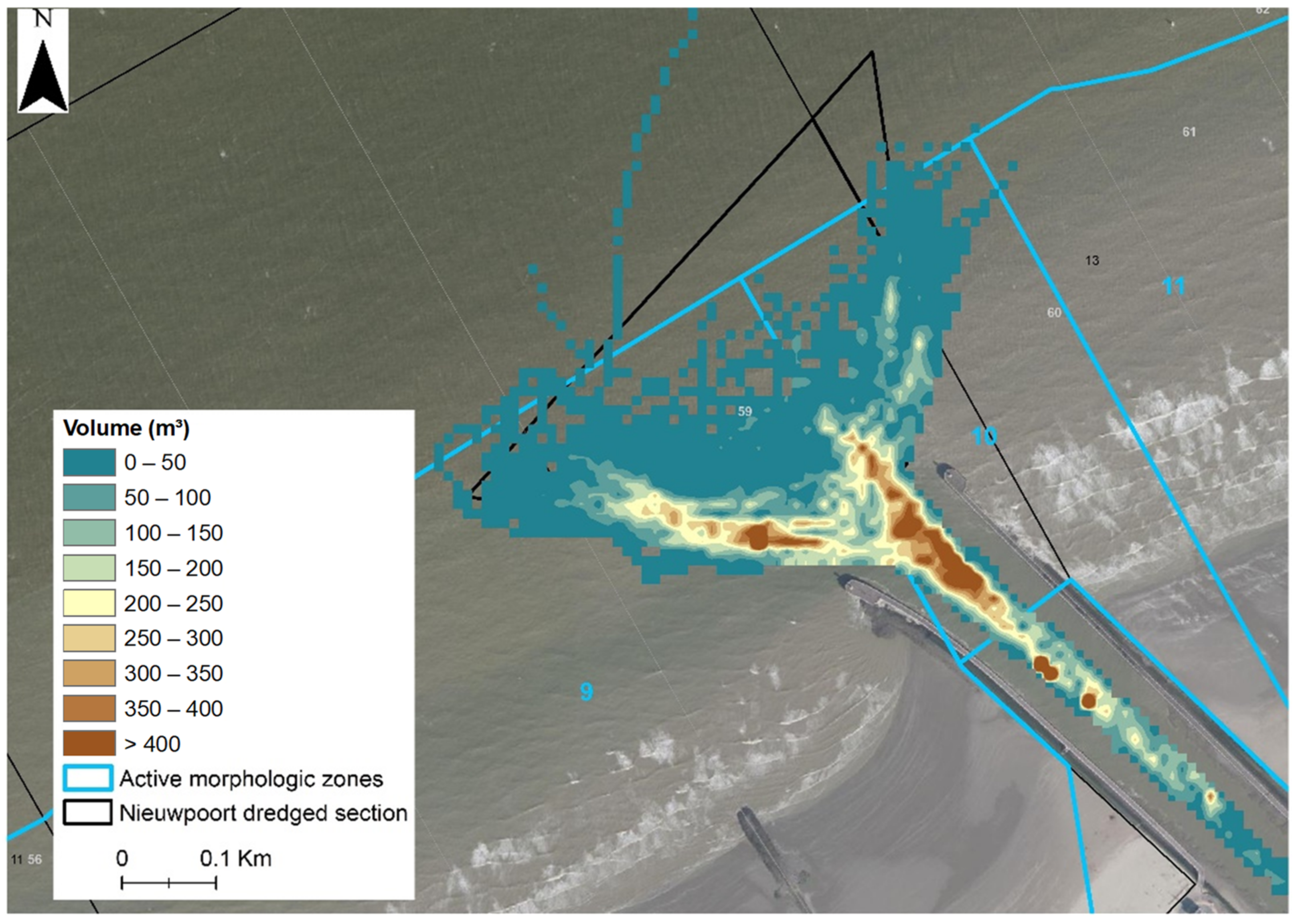
The strong erosion in Lombardsijde could be explained by what happens in the harbour entrance of Nieuwpoort. The existence of 2 harbour groins in combination with yearly dredging carried out in this harbour entrance caused erosion east of the harbour entrance. The yearly amounts of dredged material were determined from the bathymetric soundings pre- and post-dredging. On average it was 45,000 m3/year, based on data for the period 2008–2019 [8]. All this dredged material was disposed at sea, outside the active zone, so this meant that it was a loss from the beach and shoreface system. A dredging intensity map is shown to illustrate this process (Figure 7).
One can assume that sedimentation in the southwestern part of the access channel was higher compared to the northeastern side, because alongshore sand transport was primarily from southwest to northeast. Indeed, more sand was dredged at the southwest side compared to the northeast side (Figure 7).
3.2. Conceptual Model
Results of littoral drift numerical output from 2DH Scaldis-Coast in Table 3 were given in 8 transects shown in Figure 8. Transects 1, 2, 3, 4, 5 were situated west of Den Oever. Transects 6, 7, 8 were situated east of Den Oever.
The model suggested there were substantial differences between the southwestern and the northeastern part of the study area. In the southwestern part, the littoral drift was around 40,000 m3/year, while it was around 80,000 m3/year in the northeastern part. This meant that there was a large gradient at the location Den Oever. This was only partly explained by the longer active zone (cf. Figure 9). As mentioned earlier Den Oever is the location where there is a shoreface connected ridge attached to the coastline. In previous research [9,20], empirical evidence was found that a natural sand engine is located here, meaning that cross-shore sand transport occurs from offshore to the coastline via the shoreface connected ridge. Empirical evidence, in the first instance, comes from the genesis of the dunes. Wide dune areas at the Belgian coast coincide with the position of shoreface connected ridges along the Belgian coast. Before the construction of the Ostend and Zeebrugge harbours, around the year 1900, three shoreface connected ridges were present. Nowadays, only one is still present, namely at the Belgian West Coast. Considering the volume of the dunes of the Belgian West Coast and their genesis during the past ca. 900 years, an order of magnitude for the rate of coastal feeding was 135,000 m3/year [9]. The second empirical evidence was found in the shape of the coastline around Den Oever. A protrusion of 300 m in the coastline could be caused by natural feeding along the crest of the shoreface connected ridge. An estimate of 55,000 m3/year was made in previous research [20]. The most accurate quantification of this cross-shore transport was found in the output of the Scaldis-Coast sand transport model. A net transport across the seaward boundary of the active zone around Den Oever of approximately 85,000 m3/year was calculated. This is illustrated in Figure 9.
It must be noted that cross-shore sand transport by waves was, in general, not represented well in Scaldis-Coast numerical model. Only at the location of Den Oever was the transport across the depth of closure from Scaldis-Coast reliable. Here the transport directed towards the coast was the result of tidal currents combined with wave action. These processes were well represented in Scaldis-Coast.
Considering the sand balance of the study area in the study period, a growth rate of 105,000 m3/year was observed (Table 2). Furthermore, it was known that sand works contribute 35,000 m3/year of this (net result of nourishments and dredging). This suggested that 70,000 m3/year had to come from natural feeding, alongshore or cross-shore. Reliable estimates existed for the littoral drift, resulting in a net loss from the study area of 25,000 m3/year. Consequently, cross-shore feeding had to be as large as 95,000 m3/year. The proposed hypothesis is that this cross-shore feeding consists of two components. A first component at location Den Oever, coming from the crest of the shoreface connected ridge, for which the estimate from the Scaldis-Coast model was 85,000 m3/year. A second component distributed over the central part of the study area (the coastal towns of Koksijde and Nieuwpoort) coincides with the existence of the base of the shoreface connected ridge and amounted to 10,000 m3/year.
Knowledge on the large-scale sand transport in the study area could be summarized in the conceptual model and is presented in Figure 10.
The most important element was the cross-shore natural feeding via the shoreface connected ridge, indicated by the two types of red arrows. It was the source of sand for both the increase of the littoral drift from the southwest to the northeast part, as well as the progradation of the coastline in Koksijde and Nieuwpoort coastal towns. On Figure 10 the yellow arrows represent sand works resulting in gains (nourishments) or losses (dumping of dredged sand outside the active beach and shoreface zone), and the orange arrows represent the littoral drift at the western and eastern boundaries.
This conceptual model was an important improvement, compared to the often assumed zero cross-shore transport at the depth of closure, e.g., as is the case when applying Bruun rule [2]. From this model, although based on data from a limited period of time (2000–2020), one could conclude that the long-term coastline evolution of the Belgian West Coast would be influenced to a large extent by the cross-shore natural feeding from the gully-sand bank system connected to the coastline. In previous research conducted 10 years ago it was concluded that a seaward transport from the beach and foreshore system to the sea bottom would be present at the Belgian West Coast [17]. The new results presented in this paper show the opposite (landward transport). In other case studies on decadal scale coastal evolution modeling, the importance of cross-shore sand transport in relation to alongshore sand transport is stated. In [21] it was concluded that for an embayed beach in Australia, that was monitored for 30 years, cross-shore transport was more important than alongshore transport for describing the coastline rotations of this beach.
3.3. 1D Coastline Model in Unibest
3.3.1. Set Up of the Model
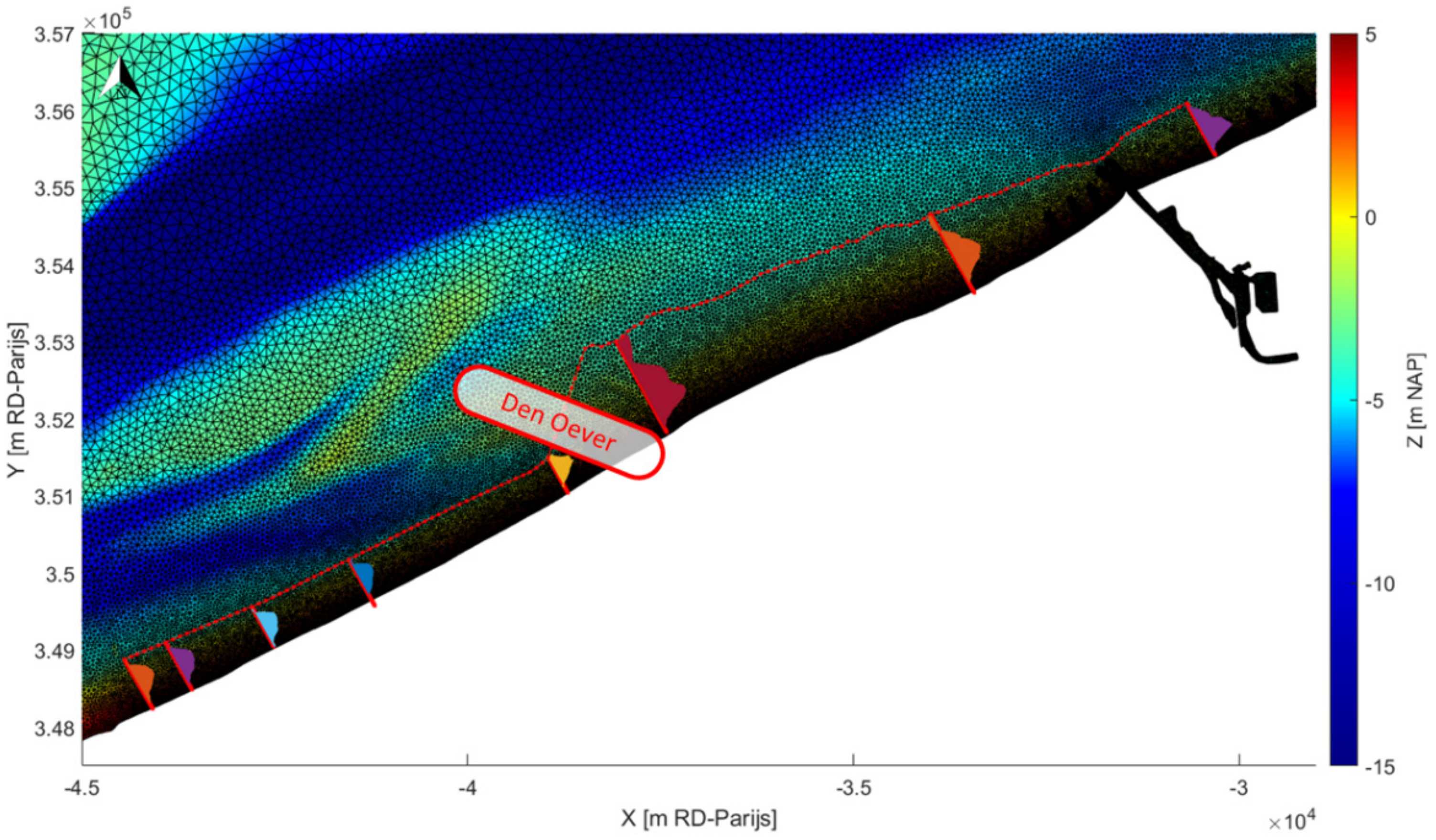
Figure 11 illustrates the schematization of the model domain that was used. The study area was subdivided into 6 sub-areas, represented by 6 cross-sections, each of which had a different profile shape, wave boundary conditions and tide boundary conditions (water level and tidal current).
For each of the 6 cross-sections Unibest calculated the longshore net sediment transport based on the wave and current climate for different coastline orientations.
The wave climate was obtained with the numerical model SWAN [22,23] by transforming the long term (10 years) offshore wave measurements (30 km offshore) to the nearshore. After obtaining modelled nearshore time series, the wave climate could be established. More details are given in [24]. An example of the wave climate is shown in Figure 12. As can be seen, the WSW to NW directions were dominant to the NNW to NE directions, resulting in a net eastward directed longshore transport.
Tidal ellipses were obtained by analyzing available measurements during a period of at least 1 month. Average maximal flood current reached ca. 0.7 m/s at two hours before high water; average maximal ebb current reached ca. 0.4 m/s. Grain size distributions were measured as well. All locations were characterized by fine to medium sand (D50 ca. 200–250 micron).
3.3.2. Littoral Drift
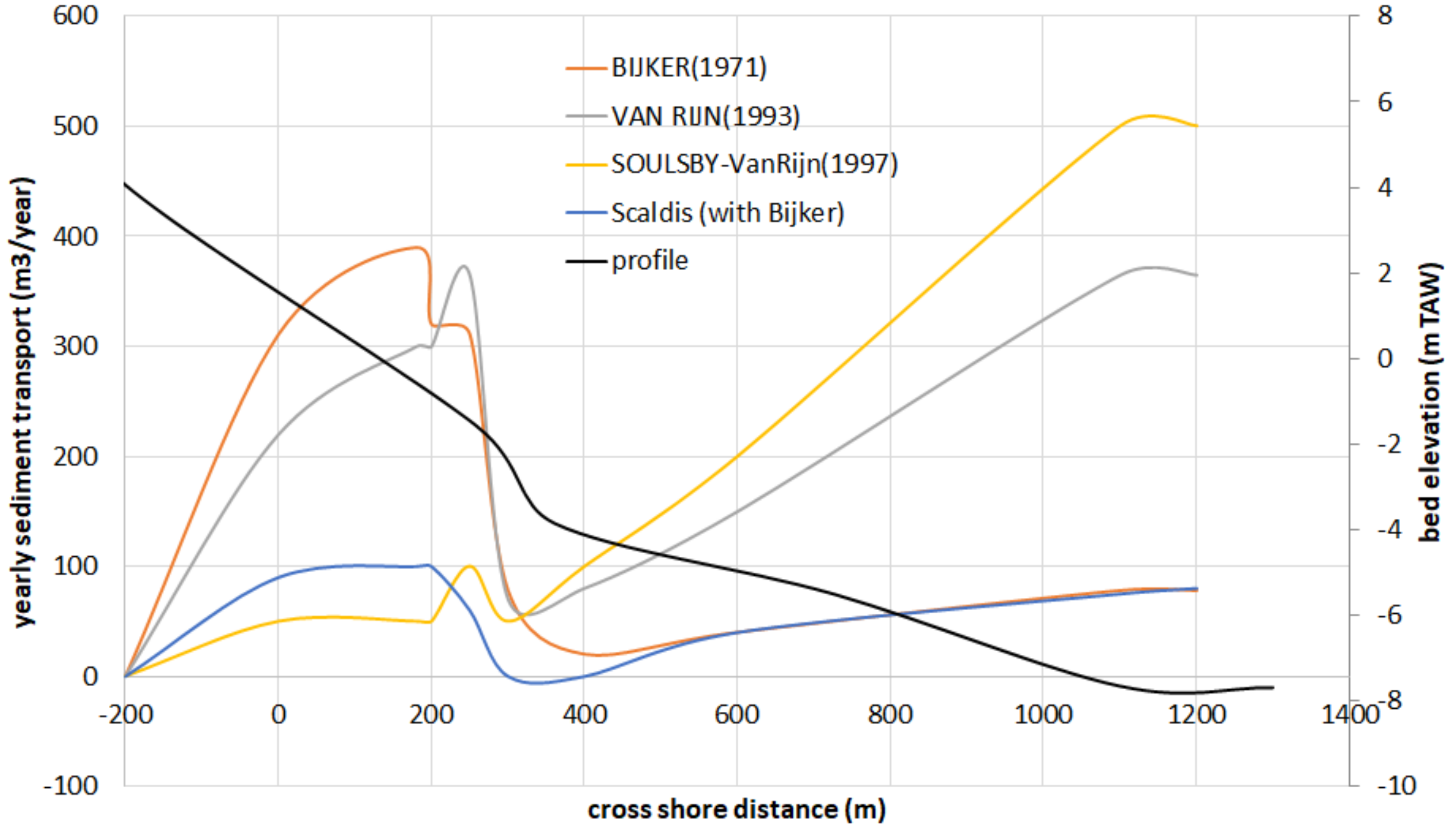
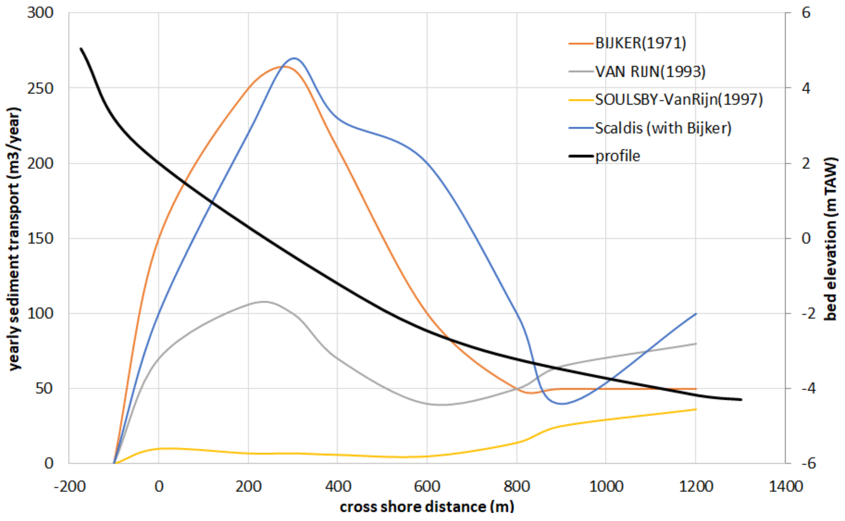
Figure 13 compares the obtained sediment transport rates for different formulations of the littoral sediment transport with the results of the Scaldis-Coast model for a relatively deep profile. Three formulations were used: Bijker [25], Van Rijn [26] and Soulsby-Van Rijn [27]. These 3 sediment transport formulations are named “Bijker”, “Van Rijn” and “Soulsby-Van Rijn” below. Although all these transport formulae could be calibrated, the used parameters should not be too different from the recommended values and also the representation of the transport should be as good as possible, both in the shallow and the deeper area, separately. Logically the formulation of Bijker fit best in the offshore part since the same formulation of Bijker was used in Scaldis-Coast. However, at the shallow beach, the LT-model with Bijker overestimated the sediment transport compared to the Scaldis-Coast model, which might be explained by an underestimation of the wave dissipation or an overestimation of the current velocities. The simplified way to incorporate tidal current velocities (a current velocity is given for a reference depth and is scaled linearly for other depths) did not permit calculating the current velocities in detail, only a change in current velocity at the reference point could be given, with equal consequences both in the shallow and deeper areas. To tackle this, tidal velocities were slightly adjusted, together with a variation of the calibration parameters in the formulae. Van Rijn and Soulsby-Van Rijn gave much higher sediment transport rates in the offshore end of the profile. In the breaker zone Van Rijn resulted in relatively high transport rates and Soulsby-Van Rijn in relatively low transport rates. This imbalance between high transport in the deeper zone and low transport in the shallow zone could not be corrected without using unrealistic calibration parameters in the transport formulae.
Figure 14 shows the results for a relatively shallow profile. In this case, the current velocities at the offshore end of the profile were much smaller. In this case, the Bijker results for both numerical models corresponded better in the whole profile. Therefore, Bijker formula was selected to use for both deep and shallow profiles.
The simplified Unibest model could not capture all complex wave and current processes. Given the complex area, with a high variation in shape of cross shore profiles and length of the profiles, it was necessary that, for each type of profile, a detailed analysis and calibration was used, using different boundary conditions for each type of profile. In this area especially the tidal current velocities had to be determined with care.
For all profiles, the sediment transport formulae and its parameters were kept constant (Bijker):
- -
- bottom roughness: 2 cm
- -
- critical deep water Hm0/h: 0.07
- -
- critical shallow water Hm0/h: 0.6
- -
- the calibration (scaling) coefficient at deep water: 2
- -
- the calibration (scaling) coefficient at shallow water: 4
Calibration was done by varying:
- -
- the current velocity: the current velocity was calculated in Unibest by scaling the reference velocity at a reference depth using the water depth. The smaller the water depth, the smaller the current velocity. However, this was not realistic. For instance, over the shallow Den Oever, higher velocities could be expected. For this reason, the current velocities were increased for profiles with a shallow shoreface. In addition, a small (up to 3 cm/s) increase/decrease of the velocities was applied (constant reduction/increase over the tidal cycle);
- -
- the wave height: the wave height at the offshore boundary was varied up to 15%;
- -
- the wave direction: as the wave direction was given with 22.5° bins, a small rotation (up to 12°) was applied;
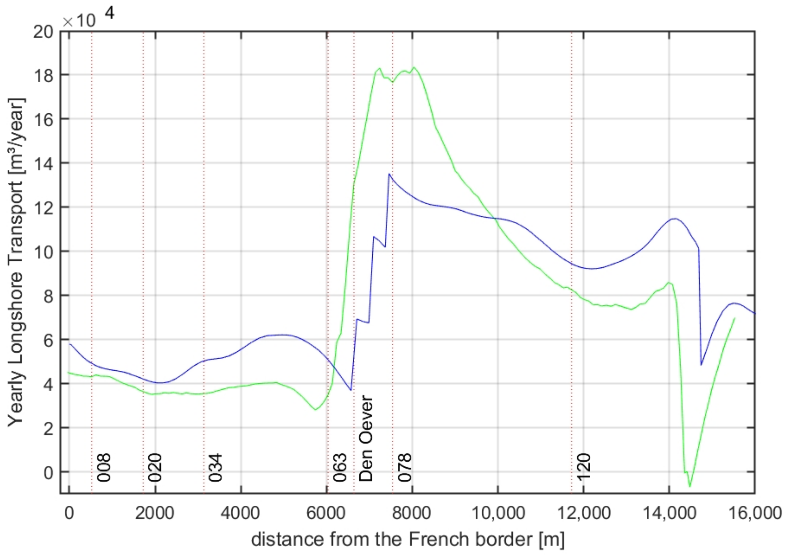
The total measured sediment budget for stretches 1 to 5 was a loss of 10,000 m3/year (cf. Table 2), while in the Scaldis Coast model a gain of 10,000 m3/year was obtained (cf. Table 3, difference between transect 5 and 1). For stretch 6 (Den Oever), Scaldis Coast gave an output of 180,000 m3/year (transect 6) and an input of 35,000 m3/year (transect 5) and a cross-shore input of 85,000 m3/year and, thus, a total output of 60,000 m3/year, while a gain of 26,000 m3/year was measured. For this reason, the target littoral drift for transect 5 was increased to 56,000 m3/year and for transect 6 decreased to 140,000 m3/year and the cross shore input was scaled to 110,000 m3/year. Figure 15 compares the obtained littoral drift along the coast in Unibest with the Scaldis Coast result. The correspondence was considered acceptable.
3.3.3. Coastline Model
After the calibration of the littoral drift for the 6 cross-sections, for each cross-section a function was available that described the littoral drift as a function of the coastline orientation. This was input for the CoastLine (CL) model. Other input of the CL-model were the coastline (the low water line) and the sources (e.g., at Den Oever where an input flux exists, due to transport over the shallow bank) and sinks (dredging in the navigation channel of Nieuwpoort). Furthermore, the most important groins (#5) and the harbour jetties of Nieuwpoort were implemented in the coastline model.
The importance of the 1D coastline model was that it established that it could be used for modelling the decadal scale evolution of the study area. Nourishment strategies to cope with sea level rise scenarios could be investigated using this model. Nevertheless, one has to take care interpreting model output, considering the simplifications of the model set-up, as is true for all kinds of models and, specifically, with morphological models. Best practice is to combine different morphological models and make conclusions based on an analysis of all model outputs, as is done by many researchers (e.g., [11,12]). Some authors have developed an integrated morphological model combining advantages of a 2DH process description and a 1D coastline schematization with an equilibrium profile concept, e.g., Q2D-morfo [28].
For the Belgian West Coast one can combine 2DH modelling using Scaldis-Coast [10]) with 1D coastline modelling, e.g., with the Unibest model presented in this paper. This is, however, outside the scope of the current contribution.
4. Discussion
Morphological interaction between the coastline and the gully-sand bank system offshore was illustrated in this case study on the Belgian West Coast. Overall a cross-shore natural feeding of 95,000 m3/year was estimated for this study area in the period 2000–2020. A quantification of the natural feeding was possible, thanks to the availability of topobathymetric monitoring data spanning several decades. Processes driving this natural feeding are related to the existence of a shoreface-connected ridge:
- a first process is related to sand transport by combined action of tidal currents and wave action near the crest of the ridge. Using the Scaldis-Coast model developed for the Belgian coast this process was simulated, resulting in a more detailed insight into the spatial distribution of this transport. Additional simulations will result in more insight in the temporal distribution.
- a second process is supposed to be related to net wave-driven cross-shore transport over the relatively shallow base of the ridge. More research into this process is needed in order to better understand the physics and to be able to reproduce this in a numerical model, resulting in more detailed knowledge on the spatial and temporal distribution of this transport.
The study showed that the concept of depth of closure does not apply at the location where the ridge connects to the shoreline (at the time scale of the study: 20 years). Indeed, the morpho-dynamics of the shoreface-connected ridge interfere with the morpho-dynamics of the coastline, so, at the intersection of these morphological features it is not possible to define a depth of closure. At this location only an artificial depth of closure could be defined by interpolating between the depth of closure lines of the neighbouring areas. In the conceptual model a relatively large sand flux from offshore to the beach area is given across this artificial depth of closure, showing that it is not actually a true depth of closure. This sand flux is of the same order of magnitude as the littoral drift in the study area, namely 105 m3/year.
It would be interesting to compare the results on cross-shore natural feeding for the Belgian West Coast to other sites with a similar setting. In the literature, morphological descriptions are given of sites with shoreface-connected ridges present, e.g., in northern France, between Calais and Dunkerque [29,30,31], in central Holland in the Netherlands [32] and Fire Island, New York [33,34]. However, quantifications of cross-shore natural feeding are rare and with a very wide uncertainty band e.g., a range between 0 and 370,000 m3/year is given for Fire Island [33].
This must be related to difficulties to measure in the field. Indirectly, one can derive a measure by closing a sand balance, e.g., in this case study for a 20-year period for an area with a coastal length of 16 km. Another method would be to have field campaigns with a duration of typically some weeks deploying instruments to measure sand transport at representative locations. Such measuring techniques are notoriously difficult and expensive. Therefore, prior to a deployment in the field, instruments to measure sand transport should be thoroughly validated in laboratory conditions. Nevertheless, the basic problem remains that it is almost impossible to measure very close (cm) to the bottom, where most sand transport takes place.
The processes of cross-shore natural feeding explain why this coastal area has shown resilience against sea level rise in the past decades. What will happen when sea level rise accelerates? The answer must be found in the large-scale morphological behaviour of the gully-sand bank system. In [35] it is stated that a critical sea level rise rate exists above which the sand bank crest height will no longer be able to grow at a pace high enough to follow sea level rise. This hypothesis is based on non-linear stability analyses using a specific morpho-dynamic model. In this context, the sand bank would drown. Then, the consequence might well be that natural feeding to the coastline would stop, resulting in drowning of the beach as well. Therefore, coastal resilience would be lost. A challenge for future research is to quantify the critical sea level rise rate for the Belgian West Coast. This should be done by developing a specific morpho-dynamic model for the gully-sand bank system as well as for the neighbouring coastline that focuses on decadal/centennial time scales.
What about the interaction of the gully-sand bank system with the coastline on these time scales? Apart from the active profile adjusting to sea level rise, according to the Bruun rule, the relation to the dunes is also an essential element. Two basic situations have to be distinguished:
- -
- in the case of progradation or stability of the coastline, fore-dune building occurs, meaning sand transport from the active beach and shoreface zone towards the dunes;
- -
- in the case of retreat of the coastline, fore-dune erosion occurs, providing sand to the active beach and shoreface zone, as well as to the inland (e.g., via blow-outs).
In a Unibest coastline model the interaction with the dunes can only be schematized by a constant sink or source. So, model software development is needed to be able to describe the more complex interaction between the active beach and shoreface zone on the one hand and the dunes on the other hand. Qualitative indications are given by the Psuty diagram [36]. According to this theory coastline progradation results in fore-dune growth, but coastline retreat can result in either fore-dune growth or fore-dune loss, depending on the rate of coastline retreat. In the case of fore-dune loss, sand transfer is partly towards the inland dunes (e.g., blowouts) and partly towards the beach.
Another suggested software development is to improve the schematization of (tidal) currents in a profile in Unibest-LT. For the Belgian coast, the tidal currents are a major force, apart from the waves.
The shoreface-connected ridge acts as a natural sand motor for the Belgian West Coast. Where the crest of the ridge connects to the coastline a local protrusion in the coastline is created, due to an accumulation of sand originating from offshore. Similar to the case of an artificial sand motor, alongshore transport distributes sand to the neighbouring coastal areas, maintaining coastal protection in a wider coastal zone.
More knowledge on cross-shore natural feeding will be crucially important for coastal protection because in the coming decades more sand will be needed to maintain the sandy coastal defences (beaches, dunes, shorefaces) under climate change. A better nourishment strategy will be found if one takes into account the natural processes of cross-shore feeding from offshore to the coastline.
5. Conclusions
This research highlights that the morphological interaction between the gully-sand bank system and the coastline at the Belgian West Coast results in a net natural feeding from offshore to the coastline. The size of this decadal sand flux is of the same order of magnitude as the littoral drift, namely 105 m3/year. Future morphological modelling should take into account this interaction, e.g., when investigating the morphological response of this coast to sea level rise. These processes are incorporated in a simplified 1D coastline model, which is able to generate predictions for the next decades, but it is best practice to combine this with 2DH modelling, and make conclusions on resilience based on an analysis of all models’ outputs.
Author Contributions
Conceptualization, methodology, writing—original draft preparation, resources, supervision, project administration, funding acquisition: T.V.; software, validation, formal analysis, investigation, data curation, visualization, writing—review and editing: A.D., A.-L.M. and K.T. All authors have read and agreed to the published version of the manuscript.
Funding
This research received no external funding.
Informed Consent Statement
Not applicable.
Acknowledgments
The authors are very grateful to the Agency for Maritime and Coastal Services-Coast Division that provided the long time series of topobathymetric monitoring as well as tide, current and wave measurements in the study area.
Conflicts of Interest
The authors declare no conflict of interest.
References
- Monbaliu, J.; Mertens, T.; Bolle, A.; Verwaest, T.; Rauwoens, P.; Toorman, E.; Troch, P.; Gruwez, V. (Eds.) CREST Final Scientific Report: Take Home Messages and Project Results; VLIZ Special Publication, 85; Flanders Marine Institute (VLIZ): Oostende, Belgium, 2020; p. 145. ISBN 978-94-920439-0-0. Available online: https://biblio.ugent.be/publication/8670329/file/8670339.pdf (accessed on 16 March 2022).
- Bruun, P. Sea-level rise as a cause of shore erosion. J. Waterw. Harb. Div. 1962, 88, 117–130. [Google Scholar] [CrossRef]
- Stive, M. How important is global warming for coastal erosion? Clim. Change 2004, 64, 27–39. [Google Scholar] [CrossRef]
- Cooper, J.A.G.; Pilkey, O.H. Sea-level rise and shoreline retreat: Time to abandon the Bruun Rule. Glob. Planet. Chang. 2004, 43, 157–171. [Google Scholar] [CrossRef]
- Deng, J.; Wu, J. Assessing the effects of shoreface profile concavity on long-term shoreline changes: An exploratory study. Geo-Mar. Lett. 2020, 40, 649–658. [Google Scholar] [CrossRef]
- Van IJzendoorn, C.O.; De Vries, S.; Hallin, C.; Hesp, P.A. Sea level rise outpaced by vertical dune toe translation on prograding coasts. Sci. Rep. 2021, 11, 12792. [Google Scholar] [CrossRef] [PubMed]
- Anthony, E.J.; Aagaard, T. The lower shoreface: Morphodynamics and sediment connectivity with the upper shoreface and beach. Earth-Sci. Rev. 2010, 210, 103334. [Google Scholar] [CrossRef]
- Houthuys, R.; Verwaest, T.; Dan, S. Morfologische Evolutie van de Vlaamse Kust tot 2019: Evolutie van de Vlaamse Kust tot 2019; Versie 2.0; WL Rapporten, 18_142_1; Waterbouwkundig Laboratorium: Antwerpen, Belgium, 2021; p. 225. [Google Scholar]
- Houthuys, R.; Vos, G.; Dan, D.; Verwaest, T. Long-Term Morphological Evolution of the Flemish Coast: Holocene, Late Middle Ages to Present. Version 1.0 FHR Reports, 14_023_1. Flanders Hydraulics Research: Antwerp. IX, 2021, 98 + 5. Available online: https://www.vliz.be/en/search-persons?module=ref&refid=347112 (accessed on 16 March 2022).
- Kolokythas, G.; De Maerschalck, B.; Wang, L.; Fonias, E.; Breugem, A. Scaldis-Coast: An integrated numerical model for the simulation of the Belgian Coast morphodynamics. Geophys. Res. Abstr. 2019, 21, EGU2019-17557. [Google Scholar]
- Nnafie, A.; De Swart, H.; Falqués, A.; Calvete, D. Long-term morphodynamics of a coupled shelf-shoreline system forced by waves and tides, a model approach. J. Geophys. Res. Earth Surf. 2021, 126, e2021JF006315. [Google Scholar] [CrossRef]
- Tonnon, P.K.; Huisman, B.J.A.; Stam, G.N.; Van Rijn, L.C. Numerical modelling of erosion rates, life span and maintenance volumes of mega nourishments. Coast. Eng. 2018, 131, 51–69. [Google Scholar] [CrossRef] [Green Version]
- Roest, B. Gecombineerde Topografie en Bathymetrie van de Belgische Kust, Geïnterpoleerd Naar Kustdwarse Raaien (1997–2019); Katholieke Universiteit Leuven (KUL): Brugge, Belgium, 2019. [Google Scholar]
- Flemish Government. Available online: https://meetnetvlaamsebanken.be/ (accessed on 1 September 2020).
- Deltares. User Manual Unibest; Deltares: Delft, The Netherlands, 2020. [Google Scholar]
- Valiente, N.G.; Masselink, G.; Scott, T.; Conley, D. Depth of Closure along an Embayed, Macro-Tidal and Exposed Coast: A Multi-Criteria Approach; Coastal Dynamics: Helsingør, Denmark, 2017; p. 185. [Google Scholar]
- Dan, D.; Vandebroek, E. A sediment budget for a highly developed coast—Belgian case. In Proceedings of the Coastal Dynamics 2017, Helsingør, Denmark, 12–16 June 2017; pp. 1376–1385. [Google Scholar]
- Hallermeier, R.J. A profile zonation for seasonal sand beaches from wave climate. Coast. Eng. 1981, 4, 253–277. [Google Scholar] [CrossRef]
- Strypsteen, G.; Dan, S.; Verwaest, T.; Roest, B.; De Wulf, A.; Bonte, D.; Rauwoens, P. Long-term dune foot morphodynamics in a developed macro-tidal environment. 2022; in press. [Google Scholar]
- Verwaest, T.; Houthuys, R.; Roest, B.; Dan, S.; Montreuil, A.-L. A coastline perturbation caused by natural feeding from a shoreface-connected ridge (headland Sint-André, Belgium). J. Coast. Res. 2020, 95, 701–705. [Google Scholar] [CrossRef]
- Harley, M.D.; Turner, I.L.; Short, A.D.; Ranasinghe, R. A re-evaluation of coastal embayment rotation: The dominance of cross-shore versus alongshore sediment transport processes, Collaroy-Narrabeen Beach, southeast Australia. J. Geophys. Res. 2011, 116, F04033. [Google Scholar] [CrossRef]
- Holthuijsen, L.H.; Booij, N.; Ris, R.C. A spectral wave model for the coastal zone. In Proceedings of the 2nd International Symposium on Ocean Wave Measurement and Analysis, New Orleans, LA, USA, 25–28 July 1993; pp. 630–641. [Google Scholar]
- SWAN Technical Documentation and User Manual Cycle III, version 40.72; Delft University of Technology: Delft, The Netherlands, 2008; Available online: https://www.fluidmechanics.tudelft.nl/swan/ (accessed on 1 June 2009).
- Doorme, S.; Verwaest, T.; Trouw, K.; Verelst, K. Determination of the wave climate for the Belgian coastal waters. In Proceedings of the 1st International SWAN Workshop, TUD, Delft, The Netherlands, 8–10 June 2009. [Google Scholar]
- Bijker, E.W. Longshore transport computations. J. Waterw. Harb. Coast. Eng. Div. 1971, 97, 687–701. [Google Scholar] [CrossRef]
- Soulsby, R. Dynamics of Marine Sands; Thomas Telford: London, UK, 1997. [Google Scholar]
- Van Rijn, L.C. Principles of Sediment Transport in Rivers, Estuaries and Coastal Seas; Aqua Publications: Amsterdam, The Netherlands, 1993. [Google Scholar]
- Arriaga, J.; Rutten, J.; Ribas, F.; Falqués, A.; Ruessink, G. Modeling the long-term diffusion and feeding capability of a mega-nourishment. Coast. Eng. 2017, 121, 1–13. [Google Scholar] [CrossRef] [Green Version]
- Héquette, A.; Aernouts, D. The influence of nearshore sand bank dynamics on shoreline evolution in a macrotidal coastal environment, Calais, Northern France. Cont. Shelf Res. 2010, 30, 1349–1361. [Google Scholar] [CrossRef]
- Latapy, A.; Héquette, A.; Pouvreau, N.; Weber, N.; Robin-Chanteloup, J.-B. Mesoscale morphological changes of nearshore sand banks since the early 19th century, and their influence on coastal dynamics, Northern France. J. Mar. Sci. Eng. 2019, 7, 73. [Google Scholar] [CrossRef] [Green Version]
- Anthony, E.J. Storms, shoreface morphodynamics, sand supply, and the accretion and erosion of coastal dune barriers in the southern North Sea. Geomorphology 2013, 199, 8–21. [Google Scholar] [CrossRef]
- Van de Meene, J.W.H.; Van Rijn, L.C. The shoreface-connected ridges along the central Dutch coast, part 2: Morphological modelling. Cont. Shelf Res. 2000, 20, 2325–2345. [Google Scholar] [CrossRef]
- Kana, T.W.; Rosati, J.D.; Traynum, S.B. Lack of evidence for onshore sediment transport from deep water at decadal time scales: Fire Island, New York. J. Coast. Res. 2011, 59, 61–75. [Google Scholar] [CrossRef]
- Safak, I.; List, J.H.; Warner, J.C.; Schwab, W.C. Persistent shoreline shape induced from offshore geologic framework: Effects of shoreface connected ridges. J. Geophys. Res. Ocean. 2017, 122, 8721–8738. [Google Scholar] [CrossRef] [Green Version]
- Nnafie, A. Formation and Long-Term Evolution of Shoreface-Connected Sand Ridges: Modeling the Effects of Sand Extraction and Sea Level Rise. Ph.D. Thesis, Institute for Marine and Atmospheric Research, Utrecht University, Utrecht, The Netherlands, 2014; p. 142. [Google Scholar]
- Psuty, N.P. The coastal foredune: A morphological basis for regional coastal dune development. In Coastal Dunes: Ecology and Conservation. Ecological Studies; Martinez, M.L., Psuty, N.P., Eds.; Springer: Berlin, Germany, 2004; Volume 171, pp. 11–28. [Google Scholar]
Figure 1.
The Belgian West Coast is situated in the south of the North Sea (indicated with a red dot on the map). It is a sandy coast with dunes, either low crested (artificial situation in coastal towns) or with a higher, natural crest.
Figure 1.
The Belgian West Coast is situated in the south of the North Sea (indicated with a red dot on the map). It is a sandy coast with dunes, either low crested (artificial situation in coastal towns) or with a higher, natural crest.

Figure 2.
Sand banks and gullies in front of the study area. The location of the study area in Belgium is shown on the small map (red rectangle).
Figure 2.
Sand banks and gullies in front of the study area. The location of the study area in Belgium is shown on the small map (red rectangle).

Figure 3.
Investigation of profile dynamics using ± yearly topobathymetric monitoring data. Example of a profile illustrating the method used. In the upper panel the location of the changepoints in the slope are shown by vertical red lines. In the lower panel the variation of the standard deviation is shown with the horizontal red lines indicating average values for the zones seaward and landward of a changepoint (vertical red line).

Figure 4.
Delineation of the active zone in the study area (from stretches 1 to 13) based on profile morpho-dynamics.
Figure 4.
Delineation of the active zone in the study area (from stretches 1 to 13) based on profile morpho-dynamics.

Figure 5.
Variability of the slope of the active beach and shoreface zone in the study area.

Figure 6.
Distinguishing three parts in the study area based on sand balances.

Figure 7.
Dredging intensity maps based on dredging data from the period 2016–2020.

Figure 8.
Location of transects defined to gather output from Scaldis-Coast on the littoral drift in the study area.
Figure 8.
Location of transects defined to gather output from Scaldis-Coast on the littoral drift in the study area.

Figure 9.
Scaldis-Coast output of sand transport across the seaward boundary of the active beach and shoreface zone in the area of Den Oever (between transects 5 and 6).
Figure 9.
Scaldis-Coast output of sand transport across the seaward boundary of the active beach and shoreface zone in the area of Den Oever (between transects 5 and 6).

Figure 10.
Conceptual model for the large-scale sand exchanges in the study area.

Figure 11.
Schematization of the study area in Unibest using 6 representative combinations of profile shape, wave boundary conditions (locations indicated with black circles) and tide boundary conditions (locations indicated with blue squares).
Figure 11.
Schematization of the study area in Unibest using 6 representative combinations of profile shape, wave boundary conditions (locations indicated with black circles) and tide boundary conditions (locations indicated with blue squares).

Figure 12.
Wave climate at Koksijde at −5 m TAW.

Figure 13.
Comparison of the sediment transport rates using different formulations in Unibest with the results of Scaldis-Coast, for a relatively deep profile.
Figure 13.
Comparison of the sediment transport rates using different formulations in Unibest with the results of Scaldis-Coast, for a relatively deep profile.

Figure 14.
Comparison of the sediment transport rates using different formulations in Unibest with the results of Scaldis-Coast, for a relatively shallow profile.
Figure 14.
Comparison of the sediment transport rates using different formulations in Unibest with the results of Scaldis-Coast, for a relatively shallow profile.

Figure 15.
Comparison of the littoral drift between Scaldis Coast (in green) and Unibest (in blue). At a distance of 6300 m the Unibest result is ca. 56,000 m3/year, at a distance of 7800 m it is ca. 140,000 m3/year.
Figure 15.
Comparison of the littoral drift between Scaldis Coast (in green) and Unibest (in blue). At a distance of 6300 m the Unibest result is ca. 56,000 m3/year, at a distance of 7800 m it is ca. 140,000 m3/year.


Table 1.
Results from the analysis of the topobathymetric profiles.
| Stretch 1 | Seaward Boundary [m TAW] | Landward Boundary [m TAW] | Height of the Active Zone [m] | Width of the Active Zone [m] |
|---|---|---|---|---|
| 1 | −3.81 | 5.55 | 9.36 | 668 |
| 2 | −3.67 | 4.60 | 8.27 | 571 |
| 3 | −4.05 | 8.85 | 12.89 | 666 |
| 4 | −4.67 | 7.96 | 12.62 | 613 |
| 5 | −4.25 | 5.94 | 10.19 | 530 |
| 6 | / * | 8.76 | / | / |
| 7 | / * | 9.72 | / | / |
| 8 | −3.02 | 6.52 | 9.54 | 851 |
| 9 | −3.57 | 5.64 | 9.21 | 1008 |
| 10 | −3.62 | 6.10 | 9.72 | 983 |
| 11 | −3.43 | 5.55 | 8.98 | 801 |
| 12 | −4.70 | 5.70 | 10.28 | 798 |
| 13 | −5.16 | 5.46 | 10.51 | 813 |
Notes: 1 The study area was subdivided in 13 stretches (shown on Figure 4). * In stretches 6 and 7 it was not possible to determine the seaward boundary.
Table 2.
Results from volumetric analysis. Sand balances for three sections (shown on Figure 6).
Table 2.
Results from volumetric analysis. Sand balances for three sections (shown on Figure 6).
| De Panne and Sint-Idesbald (West of Den Oever) | Koksijde and Nieuwpoort (between Den Oever and the Harbour) | Lombardsijde (East of the Harbour) | Total Study Area | |
|---|---|---|---|---|
| Observed growth | 20,000 m3/yr | 77,000 m3/yr | 9000 m3/yr | ca. 105,000 m3/yr |
| Nourished | 30,000 m3/yr | 11,000 m3/yr | 37,000 m3/yr | ca. 80,000 m3/yr |
| Corrected growth | −10,000 m3/yr | 66,000 m3/yr | −28,000 m3/yr | ca. 25,000 m3/yr |
| Coastal length | 6.3 km | 8.1 km | 1.2 km | 15.6 km |
| Nourishment intensity | 5 m3/m/yr | 1 m3/m/yr | 31 m3/m/yr | ca. 5 m3/m/yr |
| Corrected growth intensity | −2 m3/m/yr | +8 m3/m/yr | −23 m3/m/yr | ca. 1.5 m3/m/yr |
Table 3.
Littoral drift numerical output from Scaldis-Coast given in 8 transects in the study area.
| Transect 1 | 1 | 2 | 3 | 4 | 5 | 6 | 7 | 8 |
|---|---|---|---|---|---|---|---|---|
| Littoral drift [103 m3/year] | 45 | 43 | 36 | 35 | 35 | 180 | 80 | 70 |
Note: 1 Transect numbering is from west to east.
Publisher’s Note: MDPI stays neutral with regard to jurisdictional claims in published maps and institutional affiliations. |
© 2022 by the authors. Licensee MDPI, Basel, Switzerland. This article is an open access article distributed under the terms and conditions of the Creative Commons Attribution (CC BY) license (https://creativecommons.org/licenses/by/4.0/).
Share and Cite
MDPI and ACS Style
Verwaest, T.; Dujardin, A.; Montreuil, A.-L.; Trouw, K. Understanding Coastal Resilience of the Belgian West Coast. Water 2022, 14, 2104. https://doi.org/10.3390/w14132104
AMA Style
Verwaest T, Dujardin A, Montreuil A-L, Trouw K. Understanding Coastal Resilience of the Belgian West Coast. Water. 2022; 14(13):2104. https://doi.org/10.3390/w14132104
Chicago/Turabian StyleVerwaest, Toon, Arvid Dujardin, Anne-Lise Montreuil, and Koen Trouw. 2022. "Understanding Coastal Resilience of the Belgian West Coast" Water 14, no. 13: 2104. https://doi.org/10.3390/w14132104
Note that from the first issue of 2016, this journal uses article numbers instead of page numbers. See further details here.