
Hydrological Time Series Clustering: A Case Study of Telemetry Stations in Thailand


1
Department of Computer Engineering, Faculty of Engineering, Kasetsart University, Bangkok 10900, Thailand
2
Department of Industrial Engineering, Faculty of Engineering, Kasetsart University, Bangkok 10900, Thailand
*
Author to whom correspondence should be addressed.
Water 2022, 14(13), 2095; https://doi.org/10.3390/w14132095
Submission received: 31 May 2022
/
Revised: 22 June 2022
/
Accepted: 27 June 2022
/
Published: 30 June 2022
(This article belongs to the Section Hydrology)
Abstract
:Water level data from telemetry stations typically demonstrate diverse behaviors over time. Specific characteristics can be observed among distinct station groups that are different from others. Clustering time series data into a specified number of groups based on their similarity is an initial step for further analysis in water management analytics. Our main goal in this work is to develop a clustering framework based on a combination of feature representations, feature reduction techniques, as well as clustering algorithms. Thorough experiments on multiple combinations of these methods were conducted and compared. Based on collected water level data in Thailand, UMAP reduced representations of engineered features using HAC clustering with euclidean distance outperformed other methods. Its performance reached 0.8 Fowlkes-Mallows score. Out of 81 stations, only nine unclear cases were incorrectly clustered. Distinct behaviors with abrupt and frequent fluctuations could be perfectly identified.
1. Introduction
Water level obtained from telemetry stations is counted as time series data which is a sequence of data points occurring over some period of time. Various characteristics by nature are shared among a group of stations which are relatively different from other groups. A time series clustering task aims to separate all data points into several groups based on their similarity. In simple words, similar traits of data should be clustered together while maximizing a dissimilarity among groups. It is successfully used in broad applications ranging from biology, financial markets, weather data, and hydrometry. A great amount of previous work was conducted in the area of time series clustering as thoroughly reviewed in [1,2,3,4,5,6]. There are three main categories in the context of time series clustering. These include whole time series clustering—which is our focus in this work—sub-sequence time series clustering, and time point clustering.
According to a water management system, hydrological time series are automatically collected from telemetry stations equipped with specifically designed sensors. The collected water level data varies across stations due to multiple factors such as a geolocation, environmental factors in surroundings, and even diverse seasonal effects. Some of these data tend to behave similarly, and some behave completely different from others. Clustering these data into distinct groups is an initial step prior to further analysis in water management analytics, which includes anomaly detection and data imputation, as well as a forecasting model [7]. Due to diverse behaviors of water level data across stations, the developed models for these analytics tasks could underperform significantly. Different parameter settings for groups of stations with similar behaviors were also needed. Hence, accurately clustering similar data into distinct groups could substantially benefit the whole process of the water management analytics. In addition, data preprocessing steps prior to data visualizations or any further analysis required unique settings for diverse water level patterns. Initially clustering these data into similar groups could alleviate manual work that might be required in the current practice.
Previous work applied diverse methods and techniques to cluster hydrological time series. Pattanavijit et al. [8] proposed the linear clustering algorithm which required relatively less computational time while maintaining desirable accuracy performance compared to a traditional DBSCAN method. The large scale water level data in Thailand was used as the case study in [8]. Numerous statistical clustering methods relying on any potential similarity among hydrological time series data were explored, see [9]. Marín Celestino et al. [10] assessed groundwater quality based on K-means clustering coupled with Principal Component Analysis (PCA) and a spatial analysis. Furthermore, clustering approaches such as K-Medoids, DBScan, and x-means on water level data were generally implemented for detecting flood patterns. More recently, Li et al. [11] verified the usefulness of water depth clustering techniques such as K-means clustering, agglomerative clustering, and spectral clustering algorithms in an application of flood detection. Naranjo-Fernández et al. [12] proposed groundwater level time series clustering with static and dynamic approaches while Wunsch et al. [13] focused on feature-based clustering approaches. An ensemble modeling based on Self-Organizing Maps with a modified DS2L-Algorithm was introduced to characterize and cluster hydrographs [13]. Qiao and Li [14] relied on a linear clustering-based approach to determine Lake Water Footprint to generate water level time series based on multi-mission satellite altimetry data.
In addition, clustering time series data techniques were used in accordance with other models to tackle specific water management tasks. Han et al. [15] introduced the groundwater level modeling framework which relied on the self-organizing map (SOM)-aided stepwise clustering model. Candelieri [16] used clustering algorithms to detect water consumption patterns before applying short-term forecasting models. Similarly, Farzad and El-Shafie [17] enhanced the typical ANNs rainfall-water level data prediction model with the SOM clustering method in an unsupervised manner. Kardan Moghaddam et al. [18] instead used spatial clustering approaches in a combination with machine learning models to predict aquifer groundwater level. Not only the prediction task but clustering techniques were also combined with simulation and optimization methods to accurately simulate groundwater level data, see [19]. Moreover, effects of water level and precipitations on a reservoir landslide as a target variable were tested with two-way ANOVA coupled with the K-means clustering [20].
Additionally, some previous works involved contemporary real-life case studies of sustainability or uncertainty in hydrology using related methods. Rezaei and Vadiati [21] provided a comparative review of data-driven models for estimating river suspended sediment load. Eskandari et al. [22] proposed an integrated approach of hydrochemical, isotopic, and cluster-based methods to thoroughly investigate water evolution in a vulnerable karstic region [22]. An ensemble clustering approach was developed to assess the spatiotemporal changes in groundwater quantity and quality [23]. In addition, a combination of genetic algorithm (GA) and self-organizing map (SOM) were introduced to cluster groundwater level prior to applying the prediction model for estimating groundwater level fluctuations [24].
Another pool of research applied unsupervised clustering techniques in relevant applications with respect to ours. Weather data is one of the rich fields of time series clustering analysis. Lin et al. [25] applied the functional PCA to initially observe US weather patterns prior to implementing two types of clustering approaches. The K-means clustering algorithm was proposed to tackle rainfall and storm prediction tasks, see [26,27,28]. Oppel and Fischer [29] identified temporal distributions of rainfall events based on an unsupervised learning approach which further led to flood types correlation analysis. The time series can typically involve spatial relationships among data points. Previous works also attempted to cluster spatio-temporal data in relevant applications using various methods. Clustering approaches such as K-means and fuzzy C-means were applied with spatio-temporal data such as the dam deformation monitoring data, see [30,31]. The Density-Based Spatial Clustering of Applications with Noise (DBSCAN) with its variants were also used to determine the characteristics of earthquake clustering areas, see [32].
In this work, we focused mainly on clustering hydrological time series collected from telemetry stations. The whole time series over time from each station was considered as one data point in our analysis. We proposed the framework, which combined various feature representation methods, dimensionality reduction techniques, as well as clustering approaches. We retrieved water level time series from hydro-informatics institute (HII) as our case study. Specifically, data from 2019 at 81 telemetry stations across Thailand were selected due to their completeness. The proposed clustering framework was assessed based on a manual observation as the ground truth. The Fowlkes-Mallows Score, a common metric to evaluate the similarity among clusters, was used. A novel framework and model experiments with data application distinguish our work from others. Our main contribution is applying several components with advanced techniques to enhance the overall clustering performance. To the best of our knowledge, no previous study applied the proposed clustering algorithm pipeline on water level data locally collected in Thailand.
The paper is organized as follows. A main methodology regarding an experimental analysis, the proposed framework and evaluation metrics is thoroughly described in Section 2. The framework consists of feature representations, feature reductions, and clustering algorithms. Section 3 provides results and discussions while the conclusions are summarized in Section 4.
2. Materials and Methods
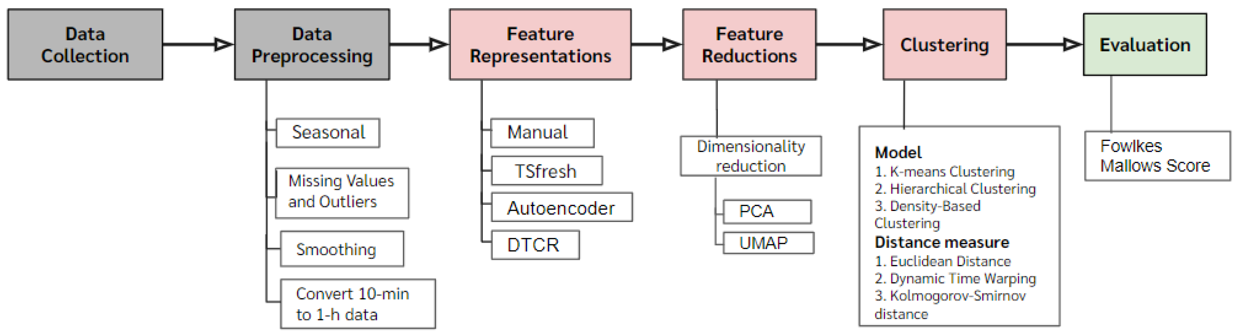
This study proposed a novel framework for clustering water level data collected from telemetry stations. These stations were equipped with sensors to monitor water level patterns over time. After the data collection process, an exploratory data analysis coupled with a data preprocessing step were performed. Our main methodology framework consisted of three main components which were feature representations, feature reductions and clustering methods. Multiple approaches of all components and their combinations were thoroughly experimented to achieve a desirable clustering performance. An evaluation step was performed at the very end to ensure the model accuracy. A flow chart of the whole process is summarized in Figure 1.
2.1. Data Collection and Data Preprocessing
According to the raw data collected from telemetry stations across Thailand, we retrieved 10-min time series water level data during 2019. We picked the range of 2019 due to its completeness. The raw data commonly contained missing values and extreme anomalies due to malfunctioned sensors or unexpected circumstances occurred at stations. Prior to performing further analysis, an exploratory observation and a data pre-processing step were needed. Data visualizations of retrieved time series data from all stations were conducted.
More recent data were relatively complete compared to long-dated historical data. We eliminated stations whose missing values were proportionally high to avoid excessive data manipulations. Extreme anomalies in the data were also removed whereas a simple interpolation function was used to impute remaining incomplete data. After this pre-processing step, there remained a total of 81 telemetry stations as depicted in Figure 2.
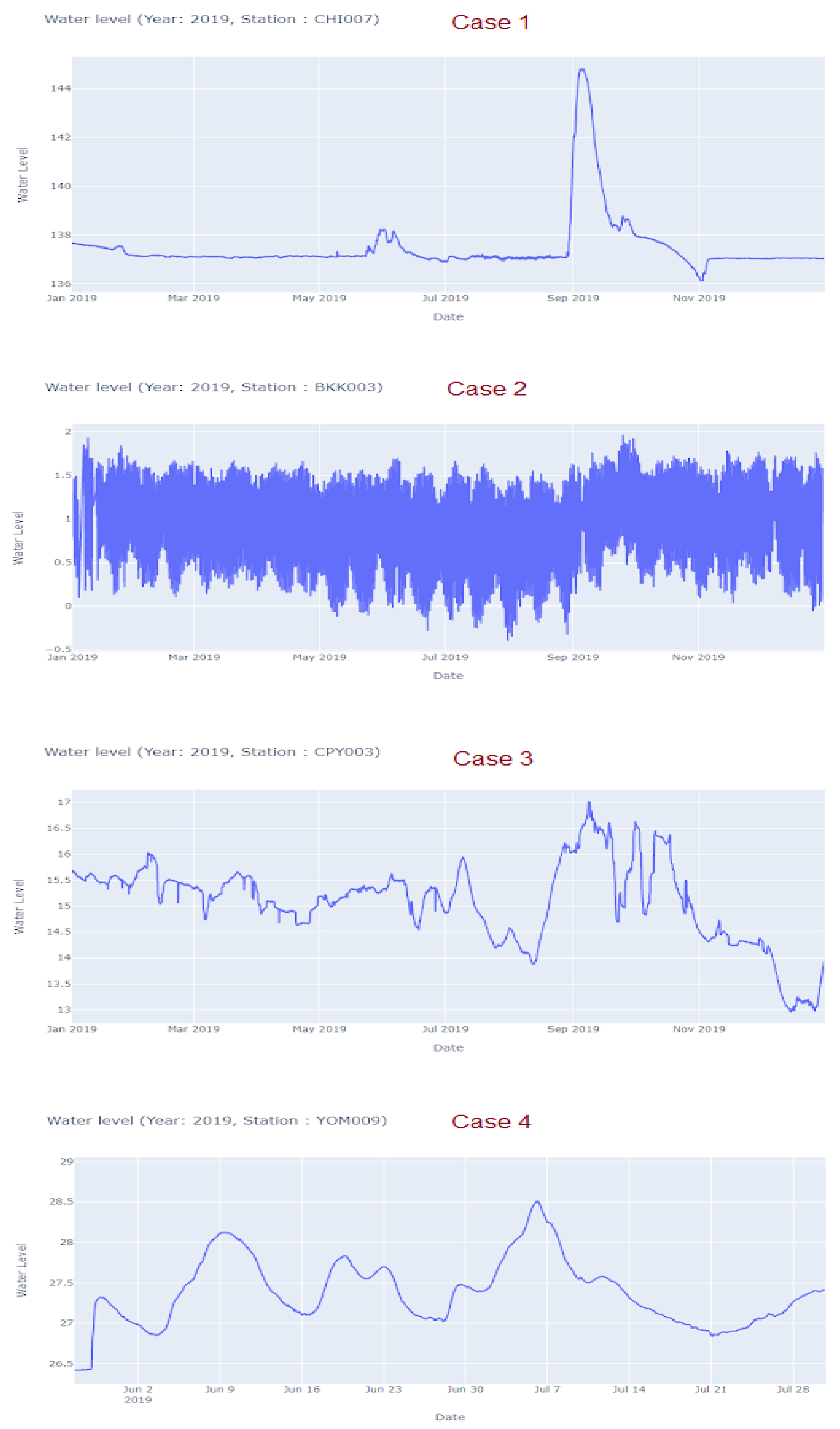
The “LowessSmoother” smoothing function from tsmoothie library was applied to the remaining data to alleviate extreme deviations or noises. The Locally Weighted Scatterplot Smoothing (Lowess), a regression analysis method to create a smooth line through a scatter plot, was applied to understand trends of any variable. Interesting trends and patterns were expected to become more distinct resulting in more insights. For the sampling protocol, we selected the first data point in each hour as a representation because variations within an hour were not significant based on the data. With an exploratory observation, diverse seasonal behaviors were observed in particular stations as depicted in Figure 3. Stations in Case 1 tended to stay stable with an abrupt peak prior to moving back down to a previous level. Highly fluctuated water level data could be clearly observed in stations within Case 2 group. While relatively random patterns with infrequent fluctuations were detected in Case 3. Stations in Case 4 exhibited more frequent upward and downward trends than those observed in Case 1 and Case 3.
2.2. Methodology
The main methodology pipeline consists of three subcomponents. According to the raw data, water level time series is counted as a sequence of data over time. In order to extract insightful information on time series behaviors, feature representations were computed. With numerous choices of feature representation techniques, a total size of extracted features were typically large. An additional step of the feature reduction through dimensionality reduction techniques was considered. Resulting features were finally fed into the clustering algorithms to group stations with similar patterns together.
2.2.1. Feature Representations
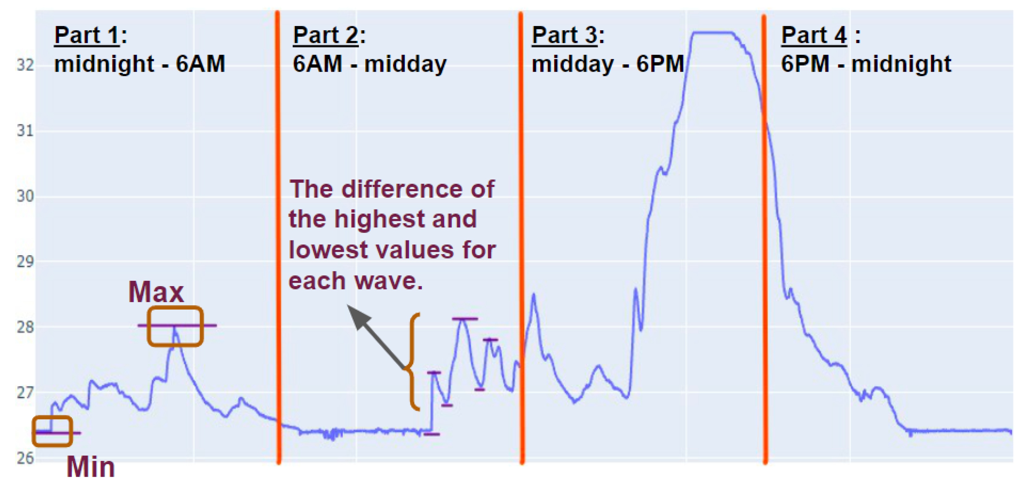
We initially extracted features based on manual observations through time series visualizations from the data exploration step. These manually extracted features represented the maximum, the minimum, and the range of the data within pre-specified windows. These window periods included midnight-6 a.m., 6 a.m.-midday, midday-6 p.m. and 6 p.m.-midnight. Figure 4 illustrates these features within specific windows.
To further enhance a list of insightful features, we adopted automated feature extraction functions from the tsfresh package (https://tsfresh.readthedocs.io/en/latest/, accessed on 1 August 2021). A large number of time series characteristics, which captured insights from raw sequential data and associated dynamics, were computed. Resulting features with a large proportion of null values, i.e., greater than 80%, were eliminated. The elimination threshold at 80% was set based on manual observations and evaluations from repeated experiments.
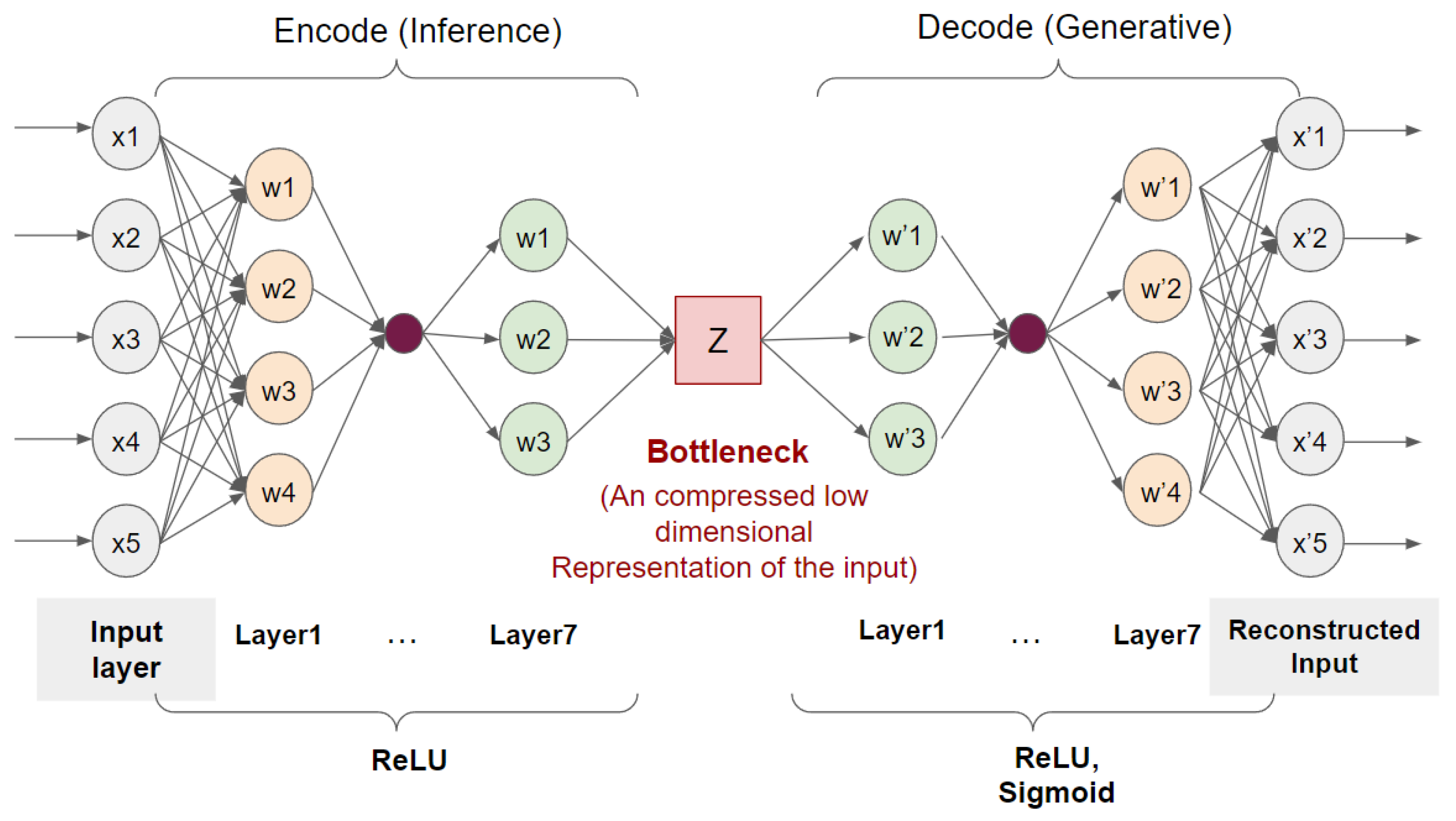
We also explored a specific type of neural networks named a sequence to sequence (seq2seq) model which aimed to learn representations from sequence data in an unsupervised manner. An autoencoder learned compressed representations of the raw data as depicted in Figure 5. It consisted of encoder and decoder sub-components. The encoder compressed the original data while the decoder attempted to reconstruct the original data based on the compacted version resulting from the encoder. Both components were stacked and trained from the raw time series data. After completing the training process, the output of the encoder was retrieved as extracted features whereas the decoder part was discarded. In addition, we adopted Deep Temporal Clustering Representation (DTCR) which incorporated the K-means clustering objective into the seq2seq model [33]. With this approach, extracted features tended to be more cluster-specific which potentially improved cluster structures later on.
2.2.2. Feature Reductions
The total number of extracted features from the previous step was typically large. Some of these features might be irrelevant, which added unnecessary noise to the data. To retrieve relatively more concise features, dimensionality reduction techniques were adopted.
First, Principal Component Analysis (PCA), a common dimensionality-reduction method was implemented. It involved an eigend composition of the covariance matrix generated from the original data to concentrate much of the information into the first few principal components and ignore irrelevant ones.
Secondly, we adopted the Uniform Manifold Approximation and Projection (UMAP), a universal purpose manifold learning and dimension reduction algorithm as a feature reduction technique (https://umap-learn.readthedocs.io/en/latest/, accessed on 1 November 2021). It attempted to optimize for the lower dimensional representation to constitute the constructed fuzzy topological representation. According to our experiments, we optimized the number of parameters in both approaches to achieve preferable performance.
2.2.3. Clustering
Three main clustering algorithms were implemented to group a set of similar objects together which were different from other groups in an unsupervised manner.
A commonly used K-means clustering method was explored. It is an iterative algorithm which assigns points to the closest cluster and re-computes clusters’ centroids repeatedly until reaching the convergence. The algorithm attempts to minimize the total variations within each cluster which implies a higher similarity of data points within the cluster.
We also implemented a Hierarchical Agglomerative Clustering (HAC) algorithm to subsequently group an individual data into a group of clusters. At the starting step, each data point was treated as an individual cluster. The closest clusters were continuously merged until only one cluster remained. Along with this method, a tree-like diagram named Dendrogram was constructed to represent the hierarchy sequence where data points were merged.
Density-Based Spatial Clustering of Applications with Noise (DBSCAN) was further considered. It is an alternative approach for cases where K-means and HAC are potentially inferior in clustering arbitrary shapes or varying densities. It is a density-based clustering algorithm which relies on clustering dense regions in a separation from relatively lower density areas. Interestingly, DBSCAN is not sensitive to outliers and does not require a predefined number of clusters.
All clustering algorithms used in this study involved similarity among data points which could be captured from various distance metrics. Three diverse distance measures were the subjects of experimentation. A euclidean distance calculated the line segment between two coordinate points. A dynamic time warping (DTW), commonly used to measure a matching similarity between two sequences, was also considered. In addition, Kolmogorov–Smirnov distance was implemented to compute the maximum difference between cumulative distribution functions (CDF) of two distinct distributions.
2.3. Evaluation Metrics
A common evaluation metric was used in this work. The Fowlkes–Mallows Score was employed to evaluate the similarity among various clustering algorithms. In particular, we initially constructed four classes of ground-truth labels based on manual annotations of the data. The score was then computed to measure the performance of each particular clustering algorithm by referencing against the ground-truth.
3. Results and Discussion
We conducted multiple experiments by varying feature representations, feature reduction techniques, and clustering algorithms as illustrated in Table 1. Within the proposed clustering framework, we observed differences among clustering algorithms and used distance measures. Among these experiments, concise representations through UMAP of hand-crafted features and tsfresh extraction features using HAC clustering with the euclidean distance provided superior performance at 0.8 Fowlkes-Mallows score.
In our experiment as shown in Table 1, we initially started with the raw data as feature representations. We compared between two commonly used clustering algorithms, namely K-means and HAC, with choices of distance measures. Large number of features generated from the tsfresh package boosted up the performance significantly against the previous two feature representations. We further incorporated auto-generated features using the autoencoder technique with diverse choices of clustering models and distance measures. Furthermore, a more complicated representation method, such as DTCR, was experimented with. Unfortunately, none of them outperformed K-means with tsfresh features. Later, we experimented on an enhancement of tsfresh features with hand-crafted feature representations. The DBScan clustering algorithm was also explored with this set of features. To further enhance the performance, we incorporated two choices of feature reduction techniques, which were UMAP and PCA, to shrink feature spaces into lower dimensions while maintaining captured information.
When the raw data was used as feature representations without further preprocessing, K-means with DTW distance measure yielded superior performance. The DTW distance played an important role in boosting the clustering performance as it captured relationships over long sequences of data relatively well. The HAC clustering method was constructed based on hierarchical relationships of data points so the DTW distance measure was not suitable. Using the Kolmogorov–Smirnov distance yielded substantially low performance. This potentially resulted from the similarity among distributions of two time series data that was not well-measured. With these undeniable results, we disregard this distance measure from further experiments. In the next step, the hand-crafted features were developed based on domain knowledge as well as manual observations of the dataset. However, these features were too simple to provide insightful information. Due to the simplicity of hand-crafted features alone, the model performance was unsurprisingly low regardless of the clustering algorithms. Extracted features from the tsfresh package were relatively great in number with enriched information. According to the experiments, K-means with euclidean distance tended to work well with these features.
Instead of these feature engineering techniques, the autoencoder based on neural networks to automatically construct feature representations was used. With the autoencoder features, the HAC clustering yielded slightly better scores compared to K-means. However, the clustering performances were still inferior to results from the tsfresh-extracted features. In terms of distance measures, clustering methods with DTW distances provided worse scores than the common euclidean distances using the autoencoder features. Auto-generated features from the autoencoder might not represent sequence relationships within the time series data well enough for the DTW distance to capture. In addition, we adopted the DTCR which relied on the seq2seq model adjusted toward clustering with k-means objective function. Results from DTCR were not as promising as other methods. Training the neural networks such as the autoencoder or DTCR with enhanced data potentially yielded more desirable results.
We further combined hand-crafted and tsfresh feature representations with various clustering methods including K-means, HAC, and DBScan. Resulting scores were slightly lower than those from the tsfresh alone. This potentially resulted from the fact that several hand-crafted features was relatively small compared to those from tsfresh. Adding a small number of features did not contribute rich enough information for the clustering model to improve. HAC is among the most suitable clustering methods with these features.
Based on our observation, the number of extracted features was significantly large especially from the tsfresh package. We then applied the dimensionality reduction techniques which are UMAP and PCA to concise these features. These two approaches were purposely designed to contain as rich important information with much less dimensions. Generally, both feature reduction methods enhanced the overall performance with some slight variations. The UMAP technique combined with HAC using the euclidean distance provided the best performance. To further observe this pattern, a scatter plot among three reduced features of UMAP is constructed as depicted in Figure 6. Each data point is color-coded with the ground-truth label. As suggested in the plot, the same color data points are flocked together with small errors. A confusion matrix corresponding to the proposed method is shown in Figure 7.
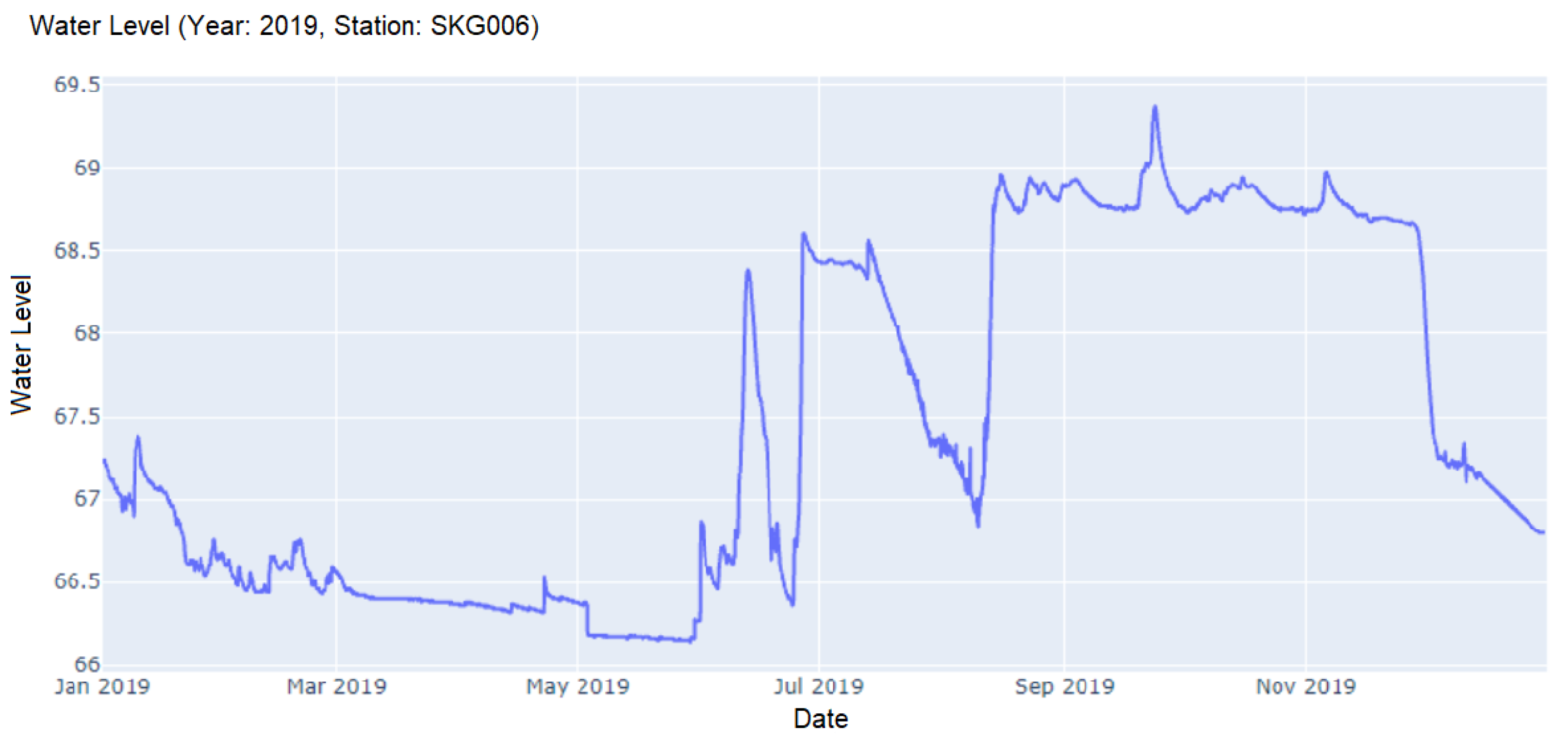
According to the confusion matrix depicted in Figure 7, the predictions of Cluster 2 were relatively accurate due to their specific characteristics with large fluctuations in the water level data. This can also be observed in a group of points in the top-left corner in Figure 6 which was color-coded as Cluster 2. These points were tightly grouped together and separate from the other clusters. The number of stations labeled as Cluster 4 was small with respect to other clusters. Our proposed clustering framework was able to correctly predict stations within this cluster even though two stations could not be recalled. From Figure 6, points belonging to Cluster 4 were mostly grouped in the bottom-right corner, see the purple dots. Our model could correctly predict these points while a few data points located in a higher position were missed. Water level data from stations in Cluster 4 tended to have relatively more frequent upward and downward abrupt trends compared to what can be observed in Cluster 3. An example of the incorrectly classified stations as illustrated in Figure 8 had slightly diverse patterns with respect to this cluster.
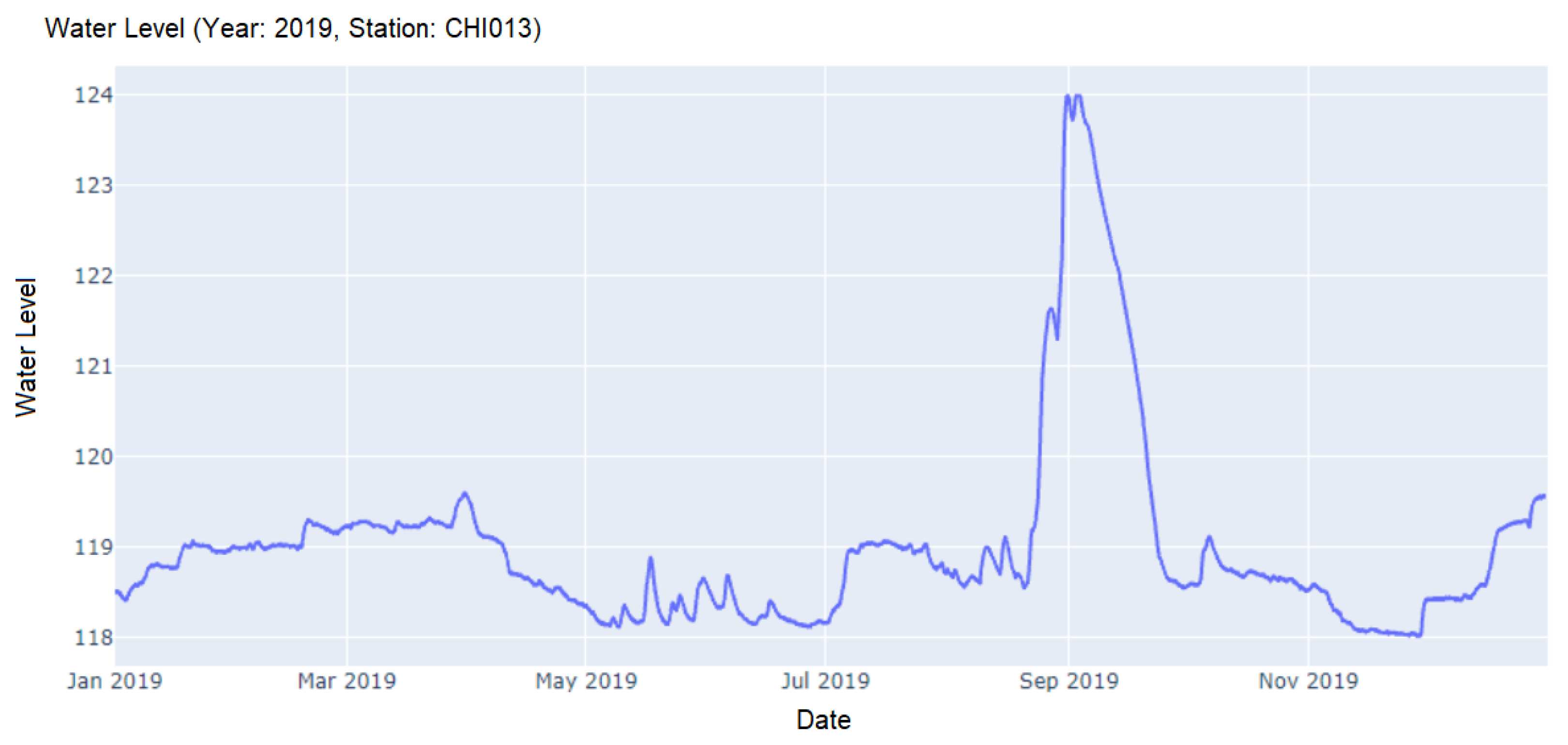
Relatively large errors were observed in Clusters 1 and 3 as illustrated in overlaps between orange and green points in Figure 6. There were six cases which were incorrectly identified as Cluster 3 by the algorithm while the true labels were Cluster 1. Both of these two clusters exhibited similar high and low tide characteristics at various timeframes. The water level at the stations in Cluster 1 tended to stay stable at the lower range with an abrupt peak at some point of time. On the other hand, the water level data within Cluster 3 typically had more fluctuations during the beginning of the year, reached its peak and stayed for a while around the middle of the year. Figure 9 depicts an example of incorrectly identified stations in Cluster 1 group which shares similar behaviors as those in Cluster 3.
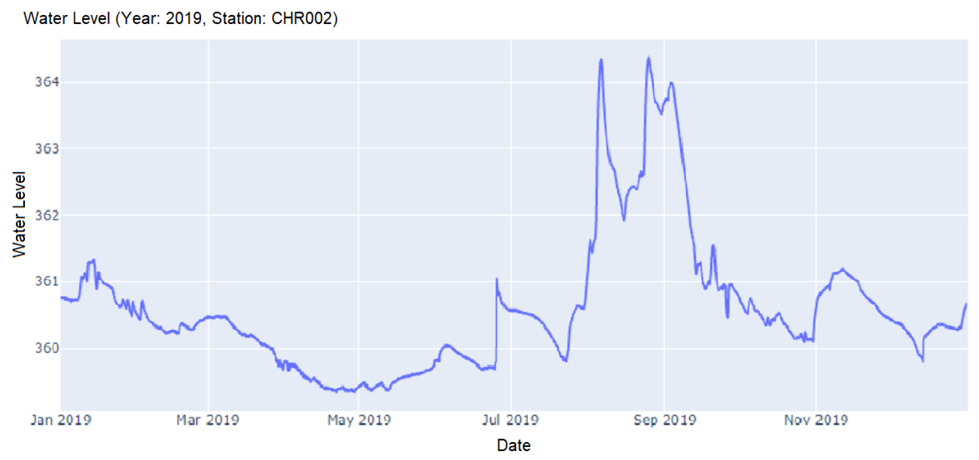
On the other hand, we observed the error case of Cluster 3 in which the algorithm was incorrectly specified as Cluster 1. From Figure 10 at station ’CHR002’, the water level data at the beginning of the year was slightly high. It then decreased to a stable level prior peaking with some fluctuations. Even though these behaviors were more similar to those observed in Cluster 3, they partially resembled patterns within Cluster 1. This observation explained the model inaccuracy. In order to enhance the model capability as our future work, we could focus on a sequence of smaller parts of the whole data to better capture finer patterns.
Apart from adjusting the granularity of focused periods of study, our proposed clustering framework currently relied on specific data preprocessing protocols such as the smoothing function and the sampling protocol. Varying these settings potentially affect the overall results. Additional work could be performed to explore other choices of these protocols. Another major limitation of our work is the application of the proposed framework on other data set collected from diverse settings or different locations. Developing a relatively more robust framework could also be a potential direction of our work. Some previous studies proposed an ensemble clustering technique which promisingly enhanced the model performance and its robustness. Alternatively, we could incorporate our proposed model with outlier detection or data manipulation tasks as the whole pipeline to enhance the water management analytics.
4. Conclusions
Thorough experiments on water level time series clustering were performed in this paper. Multiple feature representations, dimensionality reduction techniques as well as clustering methods with diverse distance measures were implemented. Enhancing an overall clustering framework of time series data through extensive experiments is our main contribution.The proposed combination of feature extractions and clustering was able to separate water level data measured at telemetry stations into distinct groups. In particular, the reduced version of multiple enriched feature representations was able to capture relationships within the time series relatively well. Stations with similar behaviors were clustered together into the same group which was diverse compared with other groups. Significantly unique behaviors such as the high fluctuations in Cluster 2 were perfectly clustered. Small errors in the proposed algorithm could be observed in groups with overlapped patterns. Clustering telemetry stations would be beneficial for further analysis on water level data.
Author Contributions
Conceptualization, P.W.; methodology, I.P. and P.W.; software, I.P.; validation, P.W.; formal analysis, I.P.; investigation, P.W.; writing—original draft preparation, I.P. and P.W.; writing—review and editing, P.W.; visualization, I.P.; supervision, P.W.; project administration, P.W. All authors have read and agreed to the published version of the manuscript.
Funding
This research was funded by Kasetsart University Research and Development Institute under the grant number FF(KU)25.64.
Institutional Review Board Statement
Not applicable.
Informed Consent Statement
Not applicable.
Data Availability Statement
Data available on request due to restrictions, e.g., privacy.
Acknowledgments
This research was supported by Kasetsart University Research and Development Institute under the grant number FF(KU)25.64 project (to P.W. author). We are also grateful to Hydro Informatics Institute (HII), Thailand for providing the water level data used in this work as well as Montri Maleewong for their insightful advice.
Conflicts of Interest
The authors declare no conflict of interest.
References
- Liao, T.W. Clustering of time series data—A survey. Pattern Recognit. 2005, 38, 1857–1874. [Google Scholar] [CrossRef]
- Kavitha, V.; Punithavalli, M. Clustering time series data stream—A literature survey. arXiv 2010, arXiv:1005.4270. [Google Scholar]
- Fu, T.C. A review on time series data mining. Eng. Appl. Artif. Intell. 2011, 24, 164–181. [Google Scholar] [CrossRef]
- Zolhavarieh, S.; Aghabozorgi, S.; Teh, Y.W. A review of subsequence time series clustering. Sci. World J. 2014, 2014, 312521. [Google Scholar] [CrossRef] [PubMed]
- Aghabozorgi, S.; Shirkhorshidi, A.S.; Wah, T.Y. Time-series clustering—A decade review. Inf. Syst. 2015, 53, 16–38. [Google Scholar] [CrossRef]
- Alqahtani, A.; Ali, M.; Xie, X.; Jones, M.W. Deep Time-Series Clustering: A Review. Electronics 2021, 10, 3001. [Google Scholar] [CrossRef]
- Kulanuwat, L.; Chantrapornchai, C.; Maleewong, M.; Wongchaisuwat, P.; Wimala, S.; Sarinnapakorn, K.; Boonya-aroonnet, S. Anomaly detection using a sliding window technique and data imputation with machine learning for hydrological time series. Water 2021, 13, 1862. [Google Scholar] [CrossRef]
- Pattanavijit, N.; Vateekul, P.; Sarinnapakorn, K. A Linear-Clustering algorithm for controlling quality of large scale water-level data in Thailand. In Proceedings of the 2015 12th International Joint Conference on Computer Science and Software Engineering (JCSSE), Songkhla, Thailand, 22–24 July 2015; pp. 269–274. [Google Scholar]
- Haaf, E.; Barthel, R. An inter-comparison of similarity-based methods for organisation and classification of groundwater hydrographs. J. Hydrol. 2018, 559, 222–237. [Google Scholar] [CrossRef]
- Marín Celestino, A.E.; Martínez Cruz, D.A.; Otazo Sánchez, E.M.; Gavi Reyes, F.; Vásquez Soto, D. Groundwater quality assessment: An improved approach to K-means clustering, principal component analysis and spatial analysis: A case study. Water 2018, 10, 437. [Google Scholar] [CrossRef] [Green Version]
- Li, J.; Hassan, D.; Brewer, S.; Sitzenfrei, R. Is Clustering Time-Series Water Depth Useful? An Exploratory Study for Flooding Detection in Urban Drainage Systems. Water 2020, 12, 2433. [Google Scholar] [CrossRef]
- Naranjo-Fernández, N.; Guardiola-Albert, C.; Aguilera, H.; Serrano-Hidalgo, C.; Montero-González, E. Clustering groundwater level time series of the exploited Almonte-Marismas aquifer in Southwest Spain. Water 2020, 12, 1063. [Google Scholar] [CrossRef] [Green Version]
- Wunsch, A.; Liesch, T.; Broda, S. Feature-based Groundwater Hydrograph Clustering Using Unsupervised Self-Organizing Map-Ensembles. Water Resour. Manag. 2022, 36, 39–54. [Google Scholar] [CrossRef]
- Qiao, G.; Li, H. Lake Water Footprint Determination Using Linear Clustering-based Algorithm and Lake Water Changes in the Tibetan Plateau from 2002 to 2020. Photogramm. Eng. Remote. Sens. 2022, 88, 371–382. [Google Scholar] [CrossRef]
- Han, J.C.; Huang, Y.; Li, Z.; Zhao, C.; Cheng, G.; Huang, P. Groundwater level prediction using a SOM-aided stepwise cluster inference model. J. Environ. Manag. 2016, 182, 308–321. [Google Scholar] [CrossRef]
- Candelieri, A. Clustering and support vector regression for water demand forecasting and anomaly detection. Water. 2017, 9, 224. [Google Scholar] [CrossRef]
- Farzad, F.; El-Shafie, A.H. Performance enhancement of rainfall pattern–water level prediction model utilizing self-organizing-map clustering method. Water Resour. Manag. 2017, 31, 945–959. [Google Scholar] [CrossRef]
- Kardan Moghaddam, H.; Ghordoyee Milan, S.; Kayhomayoon, Z.; Arya Azar, N. The prediction of aquifer groundwater level based on spatial clustering approach using machine learning. Environ. Monit. Assess. 2021, 193, 173. [Google Scholar] [CrossRef]
- Kayhomayoon, Z.; Ghordoyee Milan, S.; Arya Azar, N.; Kardan Moghaddam, H. A new approach for regional groundwater level simulation: Clustering, simulation, and optimization. Nat. Resour. Res. 2021, 30, 4165–4185. [Google Scholar] [CrossRef]
- Wu, S.; Hu, X.; Zheng, W.; He, C.; Zhang, G.; Zhang, H.; Wang, X. Effects of reservoir water level fluctuations and rainfall on a landslide by two-way ANOVA and K-means clustering. Bull. Eng. Geol. Environ. 2021, 80, 5405–5421. [Google Scholar] [CrossRef]
- Rezaei, K.; Vadiati, M. A comparative study of artificial intelligence models for predicting monthly river suspended sediment load. J. Water Land Dev. 2020, 45, 107–118. [Google Scholar]
- Eskandari, E.; Mohammadzadeh, H.; Nassery, H.; Vadiati, M.; Zadeh, A.M.; Kisi, O. Delineation of isotopic and hydrochemical evolution of karstic aquifers with different cluster-based (HCA, KM, FCM and GKM) methods. J. Hydrol. 2022, 609, 127706. [Google Scholar] [CrossRef]
- Nourani, V.; Ghaneei, P.; Kantoush, S.A. Robust clustering for assessing the spatiotemporal variability of groundwater quantity and quality. J. Hydrol. 2022, 604, 127272. [Google Scholar] [CrossRef]
- Moazamnia, M.; Hassanzadeh, Y.; Sadeghfam, S.; Nadiri, A.A. Formulating GA-SOM as a multivariate clustering tool for managing heterogeneity of aquifers in prediction of groundwater level fluctuation by SVM model. Iran. J. Sci. Technol. Trans. Civ. Eng. 2022, 46, 555–571. [Google Scholar] [CrossRef]
- Lin, C.; Yu, Y.; Wu, L.Y.; Cao, J. Unsupervised Learning on US Weather Forecast Performance. Available online: https://wiki.sfu.ca/research/cao/images/2/25/WeatherForecast.pdf (accessed on 1 May 2022).
- Li, J. Clustering and Forecasting for Rain Attenuation Time Series Data. Master’s Thesis, Computer Science, KTH, School of Information and Communication Technology (ICT), Stockholm, Sweden, 14 December 2017. [Google Scholar]
- Yovan Felix, A.; Vinay, G.S.S.; Akhik, G. K-Means cluster using rainfall and storm prediction in machine learning technique. J. Comput. Theor. Nanosci. 2019, 16, 3265–3269. [Google Scholar] [CrossRef]
- Kristiyanti, D.A.; Saputra, I.; Rina, R. Rain Prediction Clustering in Australia Using the K-Means Algorithm in the WEKA and RStudio Application. Semin. Nas. Inform. 2021, 1, 187–201. [Google Scholar]
- Oppel, H.; Fischer, S. A new unsupervised learning method to assess clusters of temporal distribution of rainfall and their coherence with flood types. Water Resour. Res. 2020, 56, e2019WR026511. [Google Scholar] [CrossRef]
- Chen, B.; Hu, T.; Huang, Z.; Fang, C. A spatio-temporal clustering and diagnosis method for concrete arch dams using deformation monitoring data. Struct. Health Monit. 2019, 18, 1355–1371. [Google Scholar] [CrossRef]
- Song, J.; Zhang, S.; Tong, F.; Yang, J.; Zeng, Z.; Yuan, S. Outlier Detection Based on Multivariable Panel Data and K-Means Clustering for Dam Deformation Monitoring Data. Adv. Civ. Eng. 2021, 2021, 3739551. [Google Scholar] [CrossRef]
- Rahmi, E.; Mundzir, M.R.; Rizaldi, S.T.; Maita, I. Comparison of DBSCAN and PCA-DBSCAN Algorithm for Grouping Earthquake Area. In Proceedings of the 2021 International Congress of Advanced Technology and Engineering, Istanbul, Turkey, 4–5 July 2021; pp. 1–5. [Google Scholar]
- Ma, Q.; Zheng, J.; Li, S.; Cottrell, G.W. Learning representations for time series clustering. In Proceedings of the Advanced in Neural Information Processing Systems, Vancouver, BC, Canada, 10–12 December 2019; pp. 3781–3791. [Google Scholar]
Figure 1.
A flow process chart.

Figure 2.
Locations of all 81 stations used as our case study.

Figure 3.
Examples of seasonal behaviors observed from the water level data within each group.

Figure 4.
Examples of manually extracted features from a particular window.

Figure 5.
A structure of the autoencoder used in our study.

Figure 6.
A scatter plot of UMAP representations with cluster labels.

Figure 7.
Confusion matrix of UMAP representations of hand-crafted features and tsfresh extraction features using HAC with euclidean distance.
Figure 7.
Confusion matrix of UMAP representations of hand-crafted features and tsfresh extraction features using HAC with euclidean distance.

Figure 8.
Station ‘SKG006’ in Cluster 4 which was incorrectly identified as Cluster 3.

Figure 9.
Station ‘CHI013’ in Cluster 1 which was incorrectly identified as Cluster 3.

Figure 10.
Station ‘CHR002’ in Cluster 3 which was incorrectly identified as Cluster 1.


Table 1.
Clustering performance.
| Feature Extractions | Clustering | Fowlkes- Mallows Score | ||
|---|---|---|---|---|
| Feature Representations | Feature Reductions | Clustering Algorithms | Distance Measures | |
| Raw data | - | K-means | Euclidean | 0.446 |
| DTW | 0.618 | |||
| Kolmogorov– Smirnov | 0.282 | |||
| HAC | Euclidean | 0.446 | ||
| Kolmogorov– Smirnov | 0.288 | |||
| Hand-crafted Features | - | K-means | Euclidean | 0.47 |
| HAC | 0.453 | |||
| Tsfresh | - | K-means | Euclidean | 0.798 |
| HAC | 0.629 | |||
| Autoencoder | - | K-means | Euclidean | 0.581 |
| DTW | 0.566 | |||
| HAC | Euclidean | 0.677 | ||
| DTW | 0.532 | |||
| DTCR | K-means | Euclidean | 0.35 | |
| Hand-crafted + Tsfresh | - | K-means | Euclidean | 0.684 |
| HAC | 0.785 | |||
| DBScan | 0.515 | |||
| UMAP | K-means | Euclidean | 0.675 | |
| HAC | 0.803 | |||
| DBScan | 0.684 | |||
| PCA | K-means | Euclidean | 0.706 | |
| HAC | 0.743 | |||
| DBScan | 0.288 | |||
Publisher’s Note: MDPI stays neutral with regard to jurisdictional claims in published maps and institutional affiliations. |
© 2022 by the authors. Licensee MDPI, Basel, Switzerland. This article is an open access article distributed under the terms and conditions of the Creative Commons Attribution (CC BY) license (https://creativecommons.org/licenses/by/4.0/).
Share and Cite
MDPI and ACS Style
Prakaisak, I.; Wongchaisuwat, P. Hydrological Time Series Clustering: A Case Study of Telemetry Stations in Thailand. Water 2022, 14, 2095. https://doi.org/10.3390/w14132095
AMA Style
Prakaisak I, Wongchaisuwat P. Hydrological Time Series Clustering: A Case Study of Telemetry Stations in Thailand. Water. 2022; 14(13):2095. https://doi.org/10.3390/w14132095
Chicago/Turabian StylePrakaisak, Intouch, and Papis Wongchaisuwat. 2022. "Hydrological Time Series Clustering: A Case Study of Telemetry Stations in Thailand" Water 14, no. 13: 2095. https://doi.org/10.3390/w14132095
Note that from the first issue of 2016, this journal uses article numbers instead of page numbers. See further details here.