
Exceptional Quantity of Water Habitats on Unreclaimed Spoil Banks
by
 ,
,
Daniela Budská
1, 
Petr Chajma
1,
Filip Harabiš
1,
Milič Solský
1,
Jana Doležalová
2 and
Jiří Vojar
1,* 1
Faculty of Environmental Sciences, Czech University of Life Sciences Prague, Kamýcká 129, Suchdol, 165 00 Prague, Czech Republic
2
Nature Conservation Agency of the Czech Republic, Administration of České Středohoří PLA, Bělehradská 1308/17, 400 01 Ústí nad Labem, Czech Republic
*
Author to whom correspondence should be addressed.
Water 2022, 14(13), 2085; https://doi.org/10.3390/w14132085
Submission received: 6 May 2022
/
Revised: 22 June 2022
/
Accepted: 27 June 2022
/
Published: 29 June 2022
(This article belongs to the Section Biodiversity and Functionality of Aquatic Ecosystems)
Abstract
:Surface mining is responsible for the large-scale destruction of affected landscapes. Simultaneously, the dumping of overburden soil on spoil banks during mining generates new landscapes, usually with heterogeneous topography. If spoil banks are not subsequently reclaimed technically (i.e., if the terrain is not leveled), considerable habitat diversity can thereby be established, consisting of numerous types of both terrestrial and water habitats. We compared the area and number of freshwater habitats between spoil banks (both technically unreclaimed and reclaimed) and the surrounding landscapes undisturbed by mining. The area of water habitats and especially their numbers per km2 were by far the greatest on unreclaimed spoil banks. Meanwhile, the quantity of water bodies on reclaimed spoil banks was about half that on non-mining landscapes. Great variety among the numerous water habitats, as indicated by their areas, depths, and proportions of aquatic vegetation on unreclaimed spoil banks, can contribute to regional landscape heterogeneity and water environment stability while providing conditions suitable for diverse taxa. The exceptional number of these water bodies can compensate for their loss in the surrounding landscape. We conclude that leaving some parts of spoil banks to spontaneous succession plays an irreplaceable role in the restoration of post-mining landscapes.
1. Introduction
The constantly intensifying impacts of anthropogenic activities that lead to habitat fragmentation and the overall degradation of natural aquatic environments have resulted in very limited availability of habitats suitable for many freshwater species [1,2,3,4,5,6]. One of the most destructive human activities is large-scale open-surface coal mining [7,8,9]. On the other hand, dumping of overburden soil on spoil banks during this process generates new and unique landscapes. If the spoil banks are not subsequently leveled by technical reclamation, considerable habitat diversity can be established [10,11,12,13]. For instance, xerothermic habitats at the higher sections of spoil banks alternate with aquatic habitats established in terrain depressions on impermeable substrates [14,15,16]. It is not surprising, therefore, that the density of water bodies present on unreclaimed spoil banks is much greater than those on sites that were technically reclaimed. Furthermore, despite the presence of several large retention reservoirs intentionally constructed on technically reclaimed spoil banks, the overall area of water habitats on unreclaimed spoil banks is also greater than on reclaimed sites [17].
In addition to supporting biodiversity (see, for example, [18,19,20,21,22,23,24]), unreclaimed spoil banks can provide other ecosystem services, including increasing water retention in the landscape [25] and serving as stepping stones for migrating species [26,27,28,29]. A number of costly measures are currently being undertaken, such as stream revitalizations and establishment of new retention basins and dams, to retain water in such landscapes, prevent the loss of freshwater habitats, and reduce the effects of drought [30]. On unreclaimed spoil banks, however, water bodies arise spontaneously in large numbers and in many different shapes and sizes without any additional costs. Unfortunately, the potential of unreclaimed spoil banks as valuable habitats and water reservoirs is often reduced substantially by the consistent application of technical reclamation [17].
Numerous studies have highlighted the importance of unreclaimed post-mining sites as habitats for endangered species, whose diversity is frequently greater at such sites than in the surrounding, often intensively managed landscape [31,32,33,34,35,36]. Because species diversity is affected by habitat heterogeneity [37,38,39], it is surprising how few studies exist that focus directly on the density and qualitative parameters of freshwater habitats occurring on post-mining sites and the sites unaffected by mining. Such studies as these tend to focus on the individual characteristics of the ponds [40,41,42,43,44,45] or on the occurrence of different taxonomic groups within water bodies [46,47,48,49,50,51], but the comparative quantity of water bodies within the wider context of the surrounding landscape has not yet been examined. Such a comparison is essential for understanding the complex importance of these post-mining sites and may help to increase the application of spontaneous succession in the reclamation process for areas affected by mining activities.
Therefore, the aim of this study was to compare the quantity and characteristics of water habitats between post-mining sites (both technically reclaimed and unreclaimed spoil banks after brown coal mining) and the surrounding landscapes. Furthermore, we wanted to determine whether the water habitats on mining sites were similar to those present in surrounding areas or if they were unique in terms of their parameters. For the purpose of generalizing the results and the possibility for their use in restoration practices, the study area covers all large spoil banks in the North Bohemian brown coal basin and all types of surrounding landscapes. Included in our study were 649 water bodies.
2. Materials and Methods
2.1. Study Area
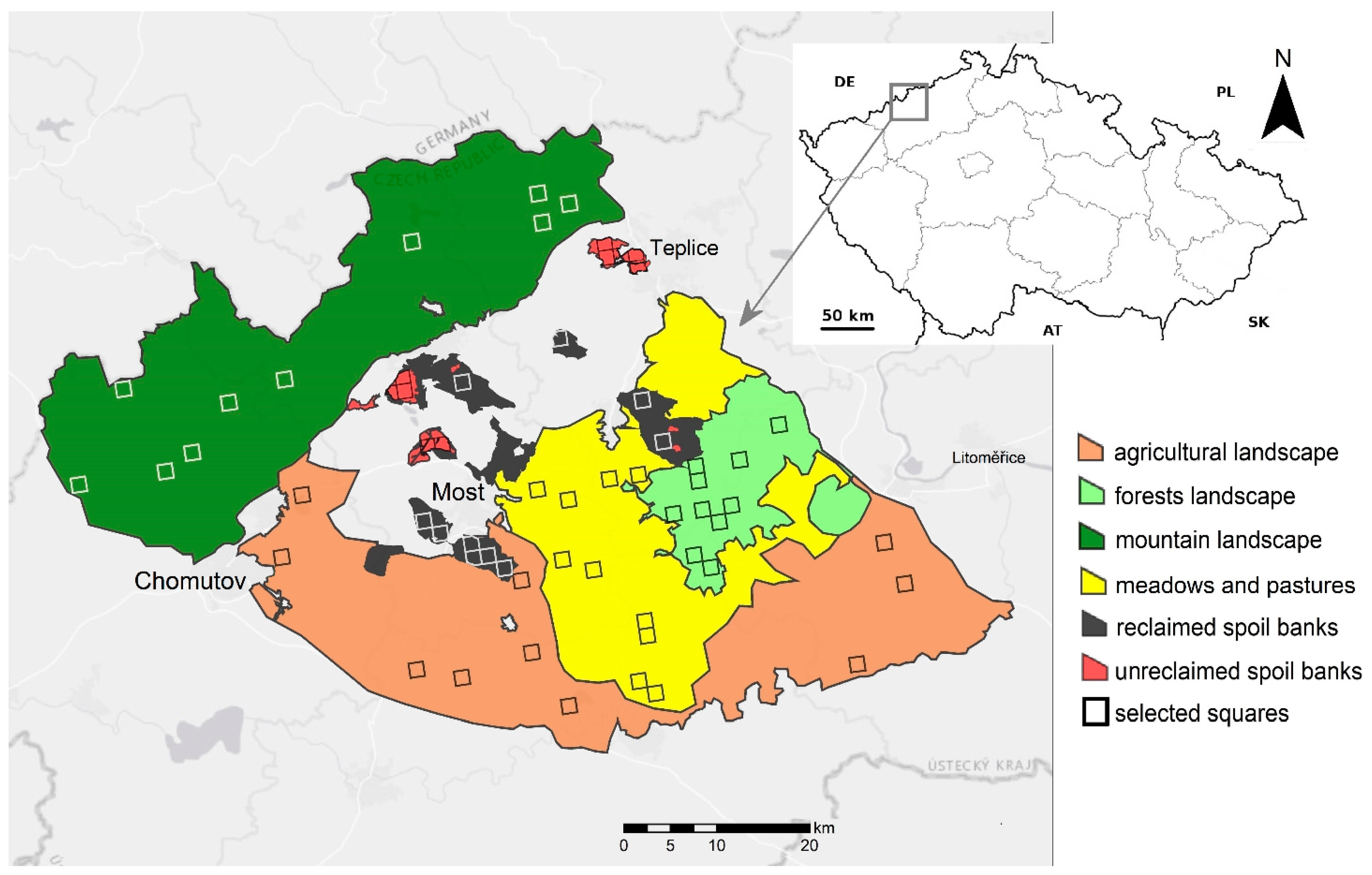
The study was carried out within the North Bohemian brown coal basin in the Czech Republic. The study sites represent the six major landscape types present in the study region: (1) technically reclaimed spoil banks, (2) technically unreclaimed spoil banks, (3) mountain range of the Ore Mountains, (4) meadows and pastures of the Central Bohemian Highlands, (5) forests of the Central Bohemian Highlands, and (6) agricultural landscape of the North Bohemian lowlands (Figure 1). The studied landscape types represent typical seminatural lands of the Czech Republic and differ in vegetation cover, land use, and altitude. The selected landscape types are described in Table 1.
2.2. Squares’ Selection and Description
Using ArcGIS 10.4 software (Esri company, Czech Republic), the area of each landscape type was divided into 1 km2 squares [52]. Squares consisting of major urban areas and squares with indeterminate landscape types (e.g., in the case of two landscape types overlapping) were excluded. Next, 10 squares per landscape were randomly selected using a random number generator in ArcGIS 10.4 [52]. Because some spoil banks, and especially those parts that were not reclaimed, are more or less restricted to an area of only a few km2, some squares were left incomplete (i.e., <1 km2). The total area of selected squares was thus reduced to 7.31 km2 for unreclaimed and 9.74 km2 for technically reclaimed spoil banks. Based upon meteorological maps and hydrological data, we interpolated average yearly precipitation for each square in ArcGIS 10.4 [52].
2.3. Water Habitat Detection and Description
We personally visited the selected squares during April and May in 2013 and determined the positions of all water habitats using Garmin eTrex 30 GPS (Product of Garmin, Czech Republic). Water habitat monitoring was conducted by a pair of experienced fieldworkers who were taking part in a similar project focused on the comparison of water habitats between reclaimed and unreclaimed spoil banks [17]. The parameters of each water body that were possibly relevant to freshwater taxa [53,54] were recorded: area, maximum depth, slope of the embankments, insolation of the water surface, and coverage of littoral vegetation. The area of larger water habitats was determined by vectorizing orthophoto maps using ArcGIS 10.4 [52]. Smaller water bodies (up to ca. 1000 m2) were measured directly in situ with a tape measure. Insolation of the water body was determined as the proportion of the water surface unshaded by the canopy of surrounding trees. The shade was measured only between 10 am and 3 pm to avoid mistakes caused by the sun’s different positions during the day [17]. Emerged and submerged vegetation (reeds, floating water plants, and flooded grasses) and other structures (e.g., flooded branches of trees) that can be used as oviposition substrates or as shelter for freshwater animals were treated as aquatic vegetation. The proportion of aquatic vegetation within each water body was estimated according to the method of Oldham et al. [55].
2.4. Statistical Analyses
Summary statistics of the visited water bodies were calculated for each type of landscape: total area of all water bodies, proportion of area covered by water bodies, mean area of water bodies, total number of water bodies, and number of water bodies per km2 (Table 2). In total, 60 squares in 6 different landscape types were analyzed: 40 squares in the landscape undisturbed by mining (non-mining areas) and 20 squares in the spoil banks. The total area covered by intensive fieldwork was 57.05 km2 (40 km2 in non-mining areas and 17.05 km2 in spoil banks).
To compare the quantity of water bodies among the six landscape types, we used generalized linear models (GLMs) with the number and total area of the water bodies in each square as responses and precipitation and landscape type as predictors. As not all squares were of the same size (see Section 2.2), square sizes measured in km2 were used as weights in the model. Due to overdispersion, the negative binomial distribution was chosen over the Poisson distribution in both cases. The total area of water bodies was strongly correlated with the number of water bodies found (rs = 0.73). Nevertheless, both are reported, as each carries a different type of information (i.e., amount of water vs. number of potential water habitats).
We used a linear mixed-effects model to compare the sizes of individual water bodies (response, log-transformed to meet the model assumptions) between the different landscape types (fixed effect). Local precipitation was used as a fixed covariate, and square identity was used as a random intercept. Furthermore, we used chi-square tests to compare the number of water bodies belonging to each level of assessed pond characteristics between the landscape types.
The interaction between landscape type and precipitation was not included in any model, as the small differences in precipitation were not expected to have varying effects on individual landscape types (as was confirmed by the preliminary data). Thus, all models were evaluated using Type II tests. To test the differences in the number and area of water bodies per km2 between the landscape types affected by mining and those that were free of mining activities, we evaluated the existing GLMs using user-defined contrasts. The p-values for the chi-square tests for all characteristics of the water bodies were corrected for multiple testing using the Holm–Bonferroni method. The analyses were conducted in R software version 4.1.2 [56] using the packages “MASS” [57], “car” [58], “lme4” [59], “lmerTest” [60], and “multcomp” [61]. The interval estimates of the coefficients from the fitted models as well as the model predictions were calculated as Bayesian 95% credible intervals (95% CrI) using the 2.5 and 97.5 percentiles of the posterior distribution of 5000 simulated values of each model parameter. The Bayesian simulations were calculated using noninformative prior distribution [62,63] through the “sim” function from the “arm” package.
3. Results
3.1. Comparison of Water Habitat Quantity among Landscape Types
The total area occupied by water habitats in all of the assessed squares was 0.93 km2, representing 1.63% of the studied area. The area of the water bodies per km2 did not differ between mining and non-mining landscapes (z = −1.42, p = 0.157), but the number of water bodies per km2 was significantly higher in the mining landscapes (z = −2.45, p = 0.014).
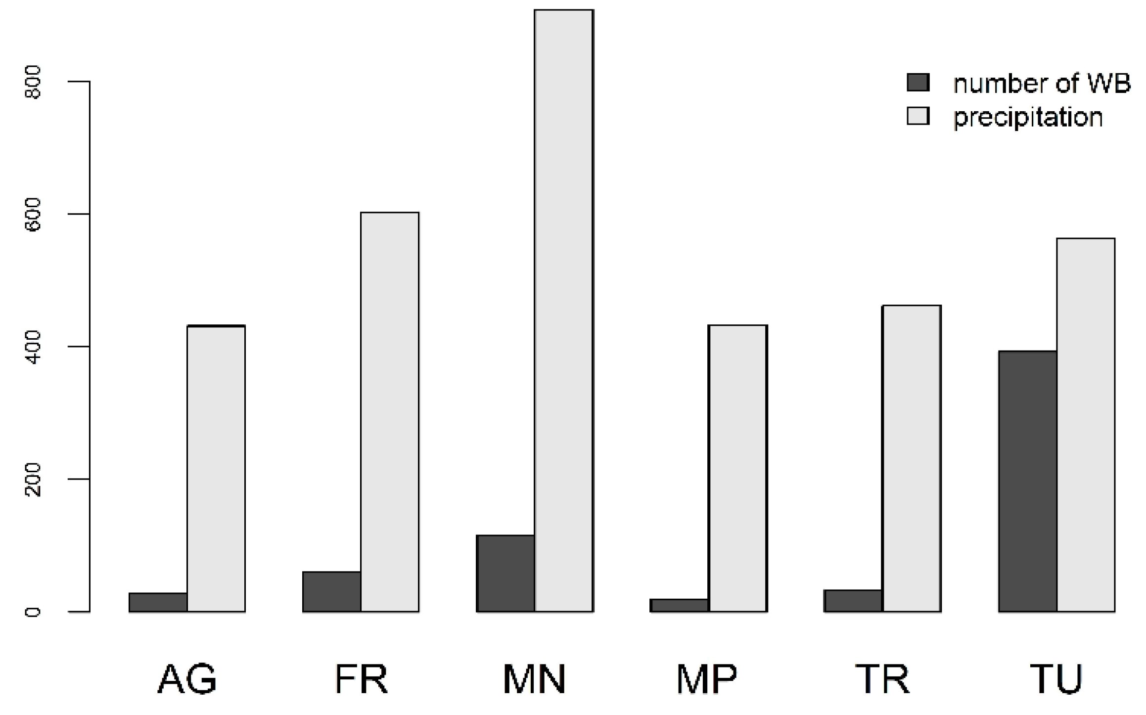
Furthermore, both the number of water bodies (χ25 = 49.37, p < 0.001) and their areas (χ25 = 16.87, p = 0.005) differed significantly among the landscapes, with precipitation affecting only the area of water bodies (χ21 = 175.216, p < 0.001) (Figure 2). The highest number of water bodies per km2 was found at unreclaimed spoil banks (95% CrI: 20.78–88.10), followed by mountains (95% CrI: 2.30–59.54), while forests (95% CrI: 3.16–11.88), agricultural landscapes (95% CrI: 1.52–8.49), reclaimed spoil banks (95% CrI: 1.33–7.91), and meadows and pastures (95% CrI: 0.77–4.65) had much fewer (Table 2). The total area of water bodies per km2 was highest in the agricultural landscapes (95% CrI: 8591.89–257,335.71 m2), followed by unreclaimed spoil banks (95% CrI: 7306.68–106,251.11 m2) and meadows and pastures (95% CrI: 3282.49–89,422.99 m2). By a large margin, the forests had the smallest area of water bodies (95% CrI: 120.05–1765.40 m2, see Table 2).
3.2. Comparison of Environmental Characteristics of Water Habitats among Landscape Types
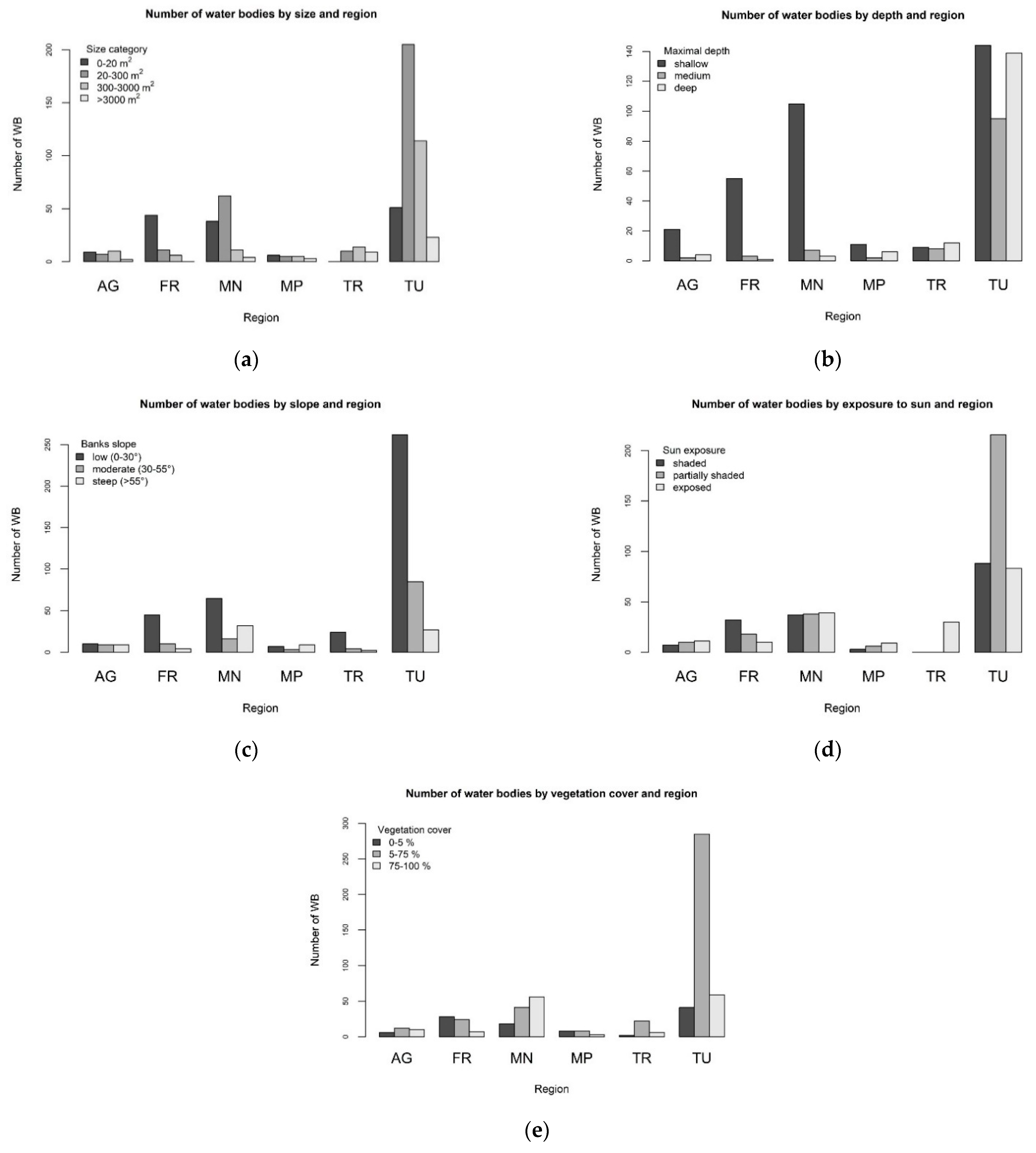
The areas of individual water bodies did not depend upon precipitation (F1 = 0.09, p = 0.77), but they did differ among landscapes (F5 = 7.70, p < 0.001). The largest mean area of the water bodies was found at reclaimed spoil banks (95% CrI: 298.60–3221.62 m2), followed by unreclaimed spoil banks (95% CrI: 114.36–488.66 m2), meadows and pastures (95% CrI: 49.50–813.03 m2) and agricultural landscapes (95% CrI: 30.40–513.67 m2). The smallest water bodies were found in forests (95% CrI: 7.71–41.89 m2) and mountains (95% CrI: 4.51–152.67 m2) (Table 3, Figure 3a).
The analysis of water body characteristics revealed significant differences in observed frequencies for all categorical variables (all p-values < 0.001, see Table 3). Water bodies occurring on spoil banks (reclaimed and unreclaimed) did not show a major difference in the numbers of shallow, medium, and deep (maximum) depths. In other landscape types, however, there was a prevalence of shallow-water habitats of maximum depth < 0.5 m (Figure 3b). Water bodies with gently sloping embankments (<30°) prevailed in most of the assessed landscapes, with the exception of meadows and pastures and agricultural landscapes (Figure 3c). The frequencies of water bodies with different levels of insolation varied greatly among the studied landscapes. At the reclaimed spoil banks, all water bodies were fully insolated. Such water bodies were also abundant in meadows and pastures. Mountain and agricultural landscapes showed a similar frequency of all types of insolation, while partially insolated water bodies prevailed on unreclaimed spoil banks. The majority of water bodies found in forests were completely shaded (Figure 3d). As for aquatic vegetation, partially covered ponds (5–75% of water surface covered by any type of aquatic vegetation) predominated in the majority of landscape types (and especially at the spoil banks), with the exception of mountains and forests (Table 3, Figure 3e).
4. Discussion
4.1. Comparison of Water Habitat Quantity among Landscape Types
Based upon our results, it is undeniable that the density of water bodies in technically unreclaimed spoil banks is many times greater than the density of aquatic habitats found in reclaimed spoil banks and in the surrounding landscape types. Moreover, the proportion of water area in unreclaimed spoil banks was the second highest among the compared landscape types. The key factor responsible for the exceptional quantity of water habitats on unreclaimed spoil banks is heterogeneous terrain topography, arising immediately after heaping of the spoil banks [11,12,14]. The originally rugged terrain surface is leveled right at the beginning of the technical reclamation. As a result, there are far fewer terrain depressions that could be filled by precipitation and, as a result, smaller numbers of water bodies in technically reclaimed spoil banks. Water bodies—usually in the form of larger retention basins—are then intentionally added to technically reclaimed spoil banks [17].
The larger and less heterogeneous water bodies created by technical reclamation can scarcely substitute for the declining supply of freshwater habitats in a regional context, consequently leading to decreased diversity of aquatic taxa (see, for example, [18,24,50]) and a reduced conservation potential of the post-mining landscapes [64,65]. Although the mere presence of aquatic habitats in large numbers does not guarantee the long-term survival of populations [53], the large supply of aquatic habitats does in and of itself increase the likelihood of there being conditions suitable for different groups of freshwater organisms [66,67,68]. Equally important is the presence of early succession stages in post-mining sites, which are noticeably lacking in the surrounding landscape [31]. With the contribution of natural succession, these systems of small wetlands can create highly valuable ecosystems [69].
In terms of the comparison of the aquatic habitat quantity among individual landscape types, the highest number of water bodies per km2 was found in unreclaimed spoil banks and mountains, while other landscape types had much fewer water habitats. Unreclaimed spoil banks and agricultural landscapes also had the highest proportions of area consisting of water habitats per km2. However, the high proportion of water area found in agricultural landscapes in our study is due to the occurrence of a single large pond, which was recorded in one square of this area and occupied almost one-third of the observed square (0.315 km2).
Few but mainly large artificial water bodies have been recorded in technically reclaimed spoil banks, with these usually serving as retention basins. These water bodies are similar in their areas and other parameters to fishponds, which were prevalent water habitats in meadows and pastures and agricultural landscapes. Most of the meadows and pastures are often located on steep slopes, where water bodies may occur only sporadically. The density of water areas is also limited in the agricultural landscape, especially in those areas of intensive agricultural management [70]. In the Czech Republic, water habitats occupy less than 1% of the agricultural landscape [71]. Kändler et al. [72] pointed out that even lower proportions of water areas exist in grasslands (0.8%) and arable land (0.3%) in the borderlands of the Czech Republic, Germany, and Poland. The overall low proportion and number of water habitats reflect the historical development of the Czech Republic’s landscape, as the majority of wetlands were drained and transformed into arable land [71]. Moreover, the occurrence of one large or a few smaller aquatic habitats per km2 is far from sufficient for most aquatic organisms [73,74,75]. Basically, these comprise isolated populations several kilometers distant from other populations, and such distance is beyond the dispersal capability of many aquatic organisms. As a result, the long-term survival of such populations is substantially limited [76,77,78].
The lowest total area of the water habitat, as measured in km2, was recorded in the forested area, but for the density of water bodies, there were close to average values among the assessed landscapes. The forests were often located on relatively steep slopes. It can be assumed that, in these conditions, there can arise only small aquatic habitats (pools, ditches, waterlogged trenches, etc.) that are flooded after snow melts but dry up later in the season, perhaps even completely. Similar small pools were also found in the mountain landscape, but their density was much higher there. As in the case of the forested landscape, however, the total area of aquatic habitat was proportionately small (about 0.2%), which is consistent with the findings of Kändler et al. [72]. On the other hand, it is undeniable that small, periodically occurring pools constitute irreplaceable habitats for many organisms and can play an important role in their persistence [79,80,81,82]. At the same time, these habitats can serve as stepping stones for dispersing individuals, thus increasing the permeability of the landscape and supporting the effective colonization of organisms into new areas [27].
Regarding the effects of precipitation, somewhat surprising is the fact that the differences in annual rainfall did not contribute to differences in the numbers of water bodies among the landscape types. The vast majority of spoil banks, and similarly the surrounding agricultural, meadow and pasture, and forest landscapes, occur in the rain shadow of the Ore Mountains, one of the driest regions of the Czech Republic [83]. It is obvious that the differences are caused much more by the topography of the individual landscape types and/or by the manner of land use.
4.2. Comparison of Environmental Characteristics of Water Habitats among Landscape Types
Despite significant differences among the observed numbers of water habitats at particular levels of pond parameters, the majority of landscape types involved water bodies across all levels of their characteristics. For most aquatic organisms, the quality of the water body determines a number of factors, namely, morphological parameters, hydrological regime, water quality and quantity, structure and composition of aquatic vegetation, presence of predators and food competitors, and many other characteristics [84]. Within this study, we focused on the area, depth, and slope of embankments, insolation of the water surface, and vegetation cover of water bodies.
The majority of freshwater invertebrates and amphibians occurring in Central Europe typically prefer smaller water habitats (ca. 500 m2) with depths to 1.5 m that allow at least partial establishment of littoral vegetation [85,86,87]. However, too-shallow water habitats are greatly influenced by fluctuations in the water level and seasonal drying [88,89], which affect the survival of eggs and aquatic larvae [90]. On the other hand, seasonal drying limits the occurrence of competitive species and fish predators [91,92]. We found that the proportions of shallow and deeper ponds were similar in both technically reclaimed and unreclaimed spoil banks, while shallow water bodies prevailed in the rest of those landscape types assessed, especially in forest and mountain landscapes. Offering a diversity of water bodies of varying depths can thus significantly enhance the biodiversity of aquatic taxa on spoil banks.
Regarding embankment slopes, steep banks can limit the development of littoral vegetation [93]. Aquatic vegetation plays a crucial role for the majority of freshwater invertebrates and amphibians, as it is their preferred oviposition substrate. Sufficient structurally heterogeneous vegetation may also significantly increase shelter possibilities for larvae and adults of those taxa [94]. Water bodies with gently sloping embankments and partially developed aquatic vegetation prevailed in most of the assessed landscapes, excluding meadow and pasture and agriculture landscapes, and thus potentially provided suitable conditions for many freshwater taxa. It is important to mention that for different groups of aquatic taxa, the optimal structure and density of macrophytic vegetation are very different [95]. For example, extensive reedbeds are very attractive to many birds, but they represent a barrier for many amphibians and do not provide enough shelter for many invertebrate species. Conversely, many species associated with early succession habitats may prefer habitats with sparse submerged vegetation.
Thus, the key factor for maintaining high biodiversity may be not only the parameters of the reservoirs but also the heterogeneity of the succession stages [20,96].
The final assessed parameter, insolation of the water surface, may have a positive effect on aquatic invertebrates and amphibians [92]. Extensive shading of the water surface reduces the water temperature and may significantly slow the development of larvae and the development of periphyton, thereby reducing food resources [97]. Fully insolated water habitats prevailed in most of the examined landscapes, with the exception of technically unreclaimed spoil banks, where there was a prevalence of partially insolated water bodies, and of forests, where the majority of water habitats were shaded.
5. Conclusions
Among all of the landscape types assessed, we found the highest number of water bodies and the second highest proportion of water area per km2 in technically unreclaimed spoil banks. Water bodies arising on technically unreclaimed spoil banks are similar with regard to their parameters to those present in the surrounding landscapes unaffected by the mining, and they do not represent unique types of freshwater habitats. The singularity of these post-mining sites lies in the exceptional numbers and variability of water bodies at different stages of succession, and these can compensate for their loss in the surrounding landscape. The potential of unreclaimed spoil banks as valuable habitats and water reservoirs is still limited, however, due to the major use of technical reclamation in the Czech Republic, directly imposed by legal measures. From this point of view, it seems far more advantageous from both an ecological and an economic point of view to give more space to spontaneous succession. On the other hand, technical reclamation as a process has an irreplaceable role in areas where “rewilding” is not entirely desirable, and therefore, the final outcome should be planned with a view to the historical past of the area concerned [98], which means the existence of extensive wetlands in our study area [9,99], and in light of ongoing environmental changes. Post-mining areas are often referred to as local biodiversity hotspots. Our study provides a very important context by comparing the density of freshwater habitats on a regional scale. However, it is true that the ecological value of a high number of aquatic habitats is to some extent directly related to mining activities. With the gradual dampening of mining activities, together with extensive drought, the impact of some invasive species or climate changes can cause many land restoration objectives to be rather untenable in the coming decades [98]. Therefore, providing space for spontaneous succession within the ecological restoration of post-mining sites and regaining at least part of the lost landscape heterogeneity seem to be more and more urgent. However, further studies should not look for the advantages and disadvantages of both approaches (spontaneous succession and technical reclamation) but should seek solutions to link the advantages of both approaches.
Author Contributions
Conceptualization, D.B., M.S., J.D. and J.V.; methodology, D.B., J.V., P.C. and F.H.; software, P.C. and D.B. and J.V.; validation, D.B., J.V. and F.H.; formal analysis, D.B.; investigation, J.V.; resources, D.B. and J.V.; data curation, D.B.; writing—original draft preparation, J.V. and D.B.; writing—review and editing, P.C., F.H., J.D. and M.S.; visualization, D.B. and P.C.; supervision, J.V.; funding acquisition, J.V., D.B. and M.S. All authors have read and agreed to the published version of the manuscript.
Funding
This research was funded by the Internal Grant Agency of the Faculty of Environmental Sciences, Czech University of Life Sciences Prague, grant numbers 20134282, 20144247, and 20154250, and by the Ministry of Education, Youth and Sports of the Czech Republic, grant number CZ.02.1.01/0.0/0.0/16_026/0008403.
Institutional Review Board Statement
Not applicable.
Informed Consent Statement
Not applicable.
Data Availability Statement
Data are available in a publicly accessible repository that does not issue DOIs. Publicly available datasets were analyzed in this study. This data can be found here.
Acknowledgments
We would like to thank Kamila Šimůnková, Petra Caltová, Barbora Havlíková, Magdalena Jílková, Lada Jakubíková, Vlaďka Jurasová, and Tomáš Kunca for their help in fieldwork.
Conflicts of Interest
The authors declare no conflict of interest.
References
- Craig, L.S.; Olden, J.D.; Arthington, A.H.; Entrekin, S.; Hawkins, C.P.; Kelly, J.J.; Kennedy, T.A.; Maitland, B.M.; Rosi, E.J.; Roy, A.H.; et al. Meeting the Challenge of Interacting Threats in Freshwater Ecosystems: A Call to Scientists and Managers. Elementa 2017, 5, 72. [Google Scholar] [CrossRef]
- Davidson, N.C. How Much Wetland Has the World Lost? Long-Term and Recent Trends in Global Wetland Area. Mar. Freshw. Res. 2014, 65, 934–941. [Google Scholar] [CrossRef]
- Dudgeon, D. Multiple Threats Imperil Freshwater Biodiversity in the Anthropocene. Curr. Biol. 2019, 29, R960–R967. [Google Scholar] [CrossRef]
- Dudgeon, D.; Arthington, A.H.; Gessner, M.O.; Kawabata, Z.I.; Knowler, D.J.; Lévêque, C.; Naiman, R.J.; Prieur-Richard, A.H.; Soto, D.; Stiassny, M.L.J.; et al. Freshwater Biodiversity: Importance, Threats, Status and Conservation Challenges. Biol. Rev. Biol. Proc. Camb. Philos. Soc. 2006, 81, 163–182. [Google Scholar] [CrossRef] [PubMed]
- Reid, A.J.; Carlson, A.K.; Creed, I.F.; Eliason, E.J.; Gell, P.A.; Johnson, P.T.J.; Kidd, K.A.; MacCormack, T.J.; Olden, J.D.; Ormerod, S.J.; et al. Emerging Threats and Persistent Conservation Challenges for Freshwater Biodiversity. Biol. Rev. 2019, 94, 849–873. [Google Scholar] [CrossRef] [PubMed] [Green Version]
- Sala, O.E.; Chapin, F.S.; Armesto, J.J.; Berlow, E.; Bloomfield, J.; Dirzo, R.; Huber-Sanwald, E.; Huenneke, L.F.; Jackson, R.B.; Kinzig, A.; et al. Global Biodiversity Scenarios for the Year 2100. Science 2000, 287, 1770–1774. [Google Scholar] [CrossRef] [PubMed]
- Kelly, M.; Allison, W.; Garman, A.; Symon, C. Mining and the Freshwater Environment; Springer Science & Business Media: Berlin/Heidelberg, Germany, 2012. [Google Scholar]
- Marcus, J.J. Mining Environment Handbook: Effects of Mining on the Environment and American Environmental Control on Mining; Imperial College Press: London, UK, 1997; ISBN 1860940293. [Google Scholar]
- Vráblíková, J.; Blažková, M.; Farský, M.; Jeřábek, M.; Seják, J.; Šoch, M.; Dejmal, I.; Jirásek, P.; Neruda, M.; Zahálka, J. Revitalizace Antropogenně Postižené Krajiny v Podkrušnohoří. Vol. 1: Přírodní a Sociálně Ekonomické Charakteristiky Disparit Průmyslové Krajiny v Podkrušnohoří; Univerzita Jana Evangelisty Purkyně v Ústí nad Labem, Fakulta Životního Prostředí: Ústí nad Labem, Czech Republic, 2008. (In Czech) [Google Scholar]
- Moradi, J.; Potocký, P.; Kočárek, P.; Bartuška, M.; Tajovský, K.; Tichánek, F.; Frouz, J.; Tropek, R. Influence of Surface Flattening on Biodiversity of Terrestrial Arthropods during Early Stages of Brown Coal Spoil Heap Restoration. J. Environ. Manag. 2018, 220, 1–7. [Google Scholar] [CrossRef]
- Prach, K. Spontaneous Succession in Central-European Man-Made Habitats: What Information Can Be Used in Restoration Practice? Appl. Veg. Sci. 2003, 6, 125–129. [Google Scholar] [CrossRef]
- Řehounek, J.; Řehounková, K.; Prach, K. Ekologická Obnova Území Narušených Těžbou Nerostných Surovin a Průmyslovými Deponiemi; Calla: České Budějovice, Czech Republic, 2010. (In Czech) [Google Scholar]
- Mojses, M.; Petrovič, F.; Bugár, G. Evaluation of Land-Use Changes as a Result of Underground Coal Mining—A Case Study on the Upper Nitra Basin, West Slovakia. Water 2022, 14, 989. [Google Scholar] [CrossRef]
- Bejček, V. Sukcese Společenstev Drobných Savců v Raných Vývojových Stádiích Výsypek v Mostecké Kotlině. Sborník Oblastního Muzea v Mostě Řada Přírodovědná 1982, 4, 61–86. [Google Scholar]
- Zelený, V. Rostliny Bílinska; Grada: Prague, Czech Republic, 1999; ISBN 80-7169-120-8. (In Czech) [Google Scholar]
- Pełka-Gościniak, J. Restoring Nature in Mining Areas of the Silesian Upland (Poland). Earth Surf. Process. Landf. 2006, 31, 1685–1691. [Google Scholar] [CrossRef]
- Doležalová, J.; Vojar, J.; Smolová, D.; Solský, M.; Kopecký, O. Technical Reclamation and Spontaneous Succession Produce Different Water Habitats: A Case Study from Czech Post-Mining Sites. Ecol. Eng. 2012, 43, 5–12. [Google Scholar] [CrossRef]
- Harabiš, F. High Diversity of Odonates in Post-Mining Areas: Meta-Analysis Uncovers Potential Pitfalls Associated with the Formation and Management of Valuable Habitats. Ecol. Eng. 2016, 90, 438–446. [Google Scholar] [CrossRef]
- Hendrychová, M.; Svobodova, K.; Kabrna, M. Mine Reclamation Planning and Management: Integrating Natural Habitats into Post-Mining Land Use. Resour. Policy 2020, 69, 101882. [Google Scholar] [CrossRef]
- Kolář, V.; Tichánek, F.; Tropek, R. Evidence-Based Restoration of Freshwater Biodiversity after Mining: Experience from Central European Spoil Heaps. J. Appl. Ecol. 2021, 58, 1921–1932. [Google Scholar] [CrossRef]
- Poláková, M.; Straka, M.; Polášek, M.; Němejcová, D. Unexplored Freshwater Communities in Post-mining Ponds: Effect of Different Restoration Approaches. Restor. Ecol. 2022, e13679. [Google Scholar] [CrossRef]
- Prach, K.; Hobbs, R.J. Spontaneous Succession versus Technical Reclamation in the Restoration of Disturbed Sites. Restor. Ecol. 2008, 16, 363–366. [Google Scholar] [CrossRef]
- Tropek, R.; Kadlec, T.; Hejda, M.; Kočárek, P.; Skuhrovec, J.; Malenovský, I.; Vodka, S.; Spitzer, L.; Baňař, P.; Konvička, M. Technical Reclamations Are Wasting the Conservation Potential of Post-Mining Sites. A Case Study of Black Coal Spoil Dumps. Ecol. Eng. 2012, 43, 13–18. [Google Scholar] [CrossRef]
- Vojar, J.; Doležalová, J.; Solský, M.; Smolová, D.; Kopecký, O.; Kadlec, T.; Knapp, M. Spontaneous Succession on Spoil Banks Supports Amphibian Diversity and Abundance. Ecol. Eng. 2016, 90, 278–284. [Google Scholar] [CrossRef]
- Kołodziej, B.; Bryk, M.; Słowińska-Jurkiewicz, A.; Otremba, K.; Gilewska, M. Soil Physical Properties of Agriculturally Reclaimed Area after Lignite Mine: A Case Study from Central Poland. Soil Tillage Res. 2016, 163, 54–63. [Google Scholar] [CrossRef]
- Cushman, S.A. Effects of Habitat Loss and Fragmentation on Amphibians: A Review and Prospectus. Biol. Conserv. 2006, 128, 231–240. [Google Scholar] [CrossRef]
- Hartel, T.; Öllerer, K. Local Turnover and Factors Influencing the Persistence of Amphibians in Permanent Ponds from the Saxon Landscapes of Transylvania. North-West. J. Zool. 2009, 5, 40–52. [Google Scholar]
- Sjögren, P.E.R. Extinction and Isolation Gradients in Metapopulations: The Case of the Pool Frog (Rana Lessonae). Biol. J. Linn. Soc. 1991, 42, 135–147. [Google Scholar] [CrossRef]
- Vojar, J. Colonization of Post-Mining Landscapes by Amphibians: A Review. Sci. Agric. Bohem. 2006, 37, 35–40. [Google Scholar]
- Vráblík, P.; Vráblíková, J.; Wildová, E. Hydrological mine reclamations in the anthropogenically affected landscape of North Bohemia. In Springer Water; Zelenakova, M., Fialová, J., Negm, A., Eds.; Springer International Publishing AG: Cham, Switzerland, 2020; pp. 203–223. ISBN 978-3-030-18362-2. [Google Scholar]
- Tropek, R.; Kadlec, T.; Karešová, P.; Spitzer, L.; Kočárek, P.; Malenovský, I.; Baňař, P.; Tuf, I.H.; Hejda, M.; Konvička, M. Spontaneous Succession in Limestone Quarries as an Effective Restoration Tool for Endangered Arthropods and Plants. J. Appl. Ecol. 2010, 47, 139–147. [Google Scholar] [CrossRef]
- Hendrychová, M.; Šálek, M.; Červenková, A. Invertebrate Communities in Man-Made and Spontaneously Developed Forests on Spoil Heaps after Coal Mining. J. Landsc. Stud. 2008, 1, 169–187. [Google Scholar]
- Hendrychová, M.; Šálek, M.; Tajovský, K.; Řehoř, M. Soil Properties and Species Richness of Invertebrates on Afforested Sites after Brown Coal Mining. Restor. Ecol. 2012, 20, 561–567. [Google Scholar] [CrossRef]
- Tischew, S.; Baasch, A.; Grunert, H.; Kirmer, A. How to Develop Native Plant Communities in Heavily Altered Ecosystems: Examples from Large-Scale Surface Mining in Germany. Appl. Veg. Sci. 2014, 17, 288–301. [Google Scholar] [CrossRef]
- Mudrák, O.; Frouz, J.; Velichová, V. Understory Vegetation in Reclaimed and Unreclaimed Post-Mining Forest Stands. Ecol. Eng. 2010, 36, 783–790. [Google Scholar] [CrossRef]
- Hodačová, D.; Prach, K. Spoil Heaps from Brown Coal Mining: Technical Reclamation versus Spontaneous Revegetation. Restor. Ecol. 2003, 11, 385–391. [Google Scholar] [CrossRef]
- Simpson, E.H. Measurement of Diversity. Nature 1949, 163, 688. [Google Scholar] [CrossRef]
- Stein, A.; Gerstner, K.; Kreft, H. Environmental Heterogeneity as a Universal Driver of Species Richness across Taxa, Biomes and Spatial Scales. Ecol. Lett. 2014, 17, 866–880. [Google Scholar] [CrossRef] [PubMed]
- Tews, J.; Brose, U.; Grimm, V.; Tielbörger, K.; Wichmann, M.C.; Schwager, M.; Jeltsch, F. Animal Species Diversity Driven by Habitat Heterogeneity/Diversity: The Importance of Keystone Structures. J. Biogeogr. 2004, 31, 79–92. [Google Scholar] [CrossRef] [Green Version]
- Kleeberg, A. The Quantification of Sulfate Reduction in Sulfate-Rich Freshwater Lakes-A Means for Predicting the Eutrophication Process of Acidic Mining Lakes? Water Air Soil Pollut. 1998, 108, 365–374. [Google Scholar] [CrossRef]
- Mays, P.A.; Edwards, G.S. Comparison of Heavy Metal Accumulation in a Natural Wetland and Constructed Wetlands Receiving Acid Mine Drainage. Ecol. Eng. 2001, 16, 487–500. [Google Scholar] [CrossRef]
- Nixdorf, B.; Hemm, M.; Schlundt, A.; Kapfer, M.; Krumbeck, H. Tagebauseen in Deutschland-Ein Überblick. 2001. Available online: https://www.baufachinformation.de/mobil/literatur/tagebauseen-in-deutschland-ein-ueberblick/2010069037823 (accessed on 4 May 2022).
- Nixdorf, B.; Krumbeck, H.; Jander, J.; Beulker, C. Comparison of Bacterial and Phytoplankton Productivity in Extremely Acidic Mining Lakes and Eutrophic Hard Water Lakes. Acta Oecol. 2003, 24, S281–S288. [Google Scholar] [CrossRef]
- Sistani, K.R.; Mays, D.A.; Taylor, R.W. Biogeochemical Characteristics of Wetlands Developed after Strip Mining for Coal. Commun. Soil Sci. Plan. 1995, 26, 3221–3229. [Google Scholar] [CrossRef]
- Taylor, J.; Middleton, B.A. Comparison of Litter Decomposition in a Natural versus Coal-Slurry Pond Reclaimed as a Wetland. Land Degrad. Dev. 2004, 15, 439–446. [Google Scholar] [CrossRef]
- Batty, L.C.; Atkin, L.; Manning, D.A.C. Assessment of the Ecological Potential of Mine-Water Treatment Wetlands Using a Baseline Survey of Macroinvertebrate Communities. Environ. Pollut. 2005, 138, 413–420. [Google Scholar] [CrossRef]
- Carrozzino, A.L. Evaluating Wildlife Response to Vegetation Restoration on Reclaimed Mine Lands in Southwestern Virginia. Master’s Thesis, Virginia Polytechnic Institute and State University, Blacksburg, Virginia, 22 April 2009. [Google Scholar]
- Carrozzino, A.L.; Stauffer, D.F.; Haas, C.A.; Zipper, C.E. Reclamation guidelines for surface mined land. In Powell River Project Research and Education Reports; Powell River Project; Virginia Tech.: Blacksburg, VA, USA, 2011; pp. 51–61. [Google Scholar]
- Lacki, M.J.; Hummer, J.W.; Webster, H.J. Diversity patterns of invertebrate fauna in cattail wetlands receiving acid mine drainage. In Proceedings of the 1990 Mining and Reclamation Conference and Exhibition, Charleston, WV, USA, 23–26 April 1990; Volume 2, pp. 365–371. [Google Scholar] [CrossRef]
- Polášková, V.; Schenková, J.; Bartošová, M.; Rádková, V.; Horsák, M. Post-Mining Calcareous Seepages as Surrogate Habitats for Aquatic Macroinvertebrate Biota of Vanishing Calcareous Spring Fens. Ecol. Eng. 2017, 109, 119–132. [Google Scholar] [CrossRef]
- Proctor, H.; Grigg, A. Aquatic Invertebrates in Final Void Water Bodies at an Open-Cut Coal Mine in Central Queensland. Aust. J. Entomol. 2006, 45, 107–121. [Google Scholar] [CrossRef]
- ESRI ArcGIS 10.4; Environmental Systems Research Institute: Redlands, CA, USA, 2018.
- Denoël, M.; Lehmann, A. Multi-Scale Effect of Landscape Processes and Habitat Quality on Newt Abundance: Implications for Conservation. Biol. Conserv. 2006, 130, 495–504. [Google Scholar] [CrossRef] [Green Version]
- Pope, S.E.; Fahrig, L.; Merriam, H.G. Landscape Complementation and Metapopulation Effects on Leopard Frog Populations. Ecology 2000, 81, 2498–2508. [Google Scholar] [CrossRef]
- Oldham, R.S.; Keeble, J.; Swan, M.; Jeffcote, M. Evaluating the Suitability of Habitat for the Great Crested Newt (Triturus Cristatus). Herpetol. J. 2000, 10, 143–156. [Google Scholar]
- R Development Core Team. R: A Language and Environment for Statistical Computing; Foundation for Statistical Computing: Vienna, Austria, 2021. [Google Scholar]
- Venables, W.N.; Ripley, B.D. Modern Applied Statistics with S; Statistics and Computing; Springer: New York, NY, USA, 2002; ISBN 978-1-4419-3008-8. [Google Scholar]
- Fox, J.; Weisberg, S.; Price, B.; Adler, D.; Bates, D.; Baud-Bovy, G.; Bolker, B. Car: Companion to Applied Regression; R package Version 3.0–3; Sage: Thousand Oaks, CA, USA, 2019; Available online: https://CRAN.R-project.org/package=car (accessed on 1 May 2022).
- Bates, D.; Mächler, M.; Bolker, B.M.; Walker, S.C. Fitting Linear Mixed-Effects Models Using Lme4. J. Stat. Softw. 2015, 67, 1–48. [Google Scholar] [CrossRef]
- Kuznetsova, A.; Brockhoff, P.B.; Christensen, R.H.B. LmerTest Package: Tests in Linear Mixed Effects Models. J. Stat. Softw. 2017, 82, 1–26. [Google Scholar] [CrossRef] [Green Version]
- Hothorn, T.; Bretz, F.; Westfall, P. Simultaneous Inference in General Parametric Models. Biom. J. 2008, 50, 346–363. [Google Scholar] [CrossRef] [Green Version]
- Gelman, A.; Hill, J. Data Analysis Using Regression and Multilevel/Hierarchical Models; Cambridge University Press: Cambridge, UK, 2006. [Google Scholar]
- Gelman, A.; Su, Y.-S. Arm: Data Analysis Using Regression and Multilevel/Hierarchical Models; R Package Version 1.12–2; Cambridge University Press: Cambridge, UK, 2021. [Google Scholar]
- Harabiš, F.; Dolný, A. Human Altered Ecosystems: Suitable Habitats as Well as Ecological Traps for Dragonflies (Odonata): The Matter of Scale. J. Insect Conserv. 2012, 16, 121–130. [Google Scholar] [CrossRef]
- Tropek, R.; Hejda, M.; Kadlec, T.; Spitzer, L. Local and Landscape Factors Affecting Communities of Plants and Diurnal Lepidoptera in Black Coal Spoil Heaps: Implications for Restoration Management. Ecol. Eng. 2013, 57, 252–260. [Google Scholar] [CrossRef]
- Marsh, D.M.; Fegraus, E.H.; Harrison, S. Effects of Breeding Pond Isolation on the Spatial and Temporal Dynamics of Pond Use by the Tungara Frog, Physalaemus pustulosus. J. Anim. Ecol. 1999, 68, 804–814. [Google Scholar] [CrossRef]
- Vos, C.; Stumpel, A.H.P. Comparison of Habitat-Isolation Parameters in Relation to Fragmented Distribution Patterns in the Tree Frog (Hyla Arborea). Landsc. Ecol. 1996, 11, 203–214. [Google Scholar] [CrossRef]
- Zanini, F. Amphibian Conservation in Human Shaped Environments: Landscape Dynamics, Habitat Modeling and Metapopulation Analyses. Ph.D. Thesis, École Plytechnique Fédérale De Lausanne, Lausanne, Switzerland, 29 September 2006. [Google Scholar]
- McCullough, C.D.; van Etten, E.J.B. Ecological Restoration of Novel Lake Districts: New Approaches for New Landscapes. Mine Water Environ. 2011, 30, 312–319. [Google Scholar] [CrossRef] [Green Version]
- Tlapáková, L. Agricultural Drainage Systems in the Czech Landscape-Identification and Functionality Assessment by Means of Remote Sensing. Europ. Countrys. 2017, 9, 77–98. [Google Scholar] [CrossRef] [Green Version]
- Skaloš, J.; Weber, M.; Lipský, Z.; Trpáková, I.; Šantrůčková, M.; Uhlířová, L.; Kukla, P. Using Old Military Survey Maps and Orthophotograph Maps to Analyse Long-Term Land Cover Changes-Case Study (Czech Republic). Appl. Geogr. 2011, 31, 426–438. [Google Scholar] [CrossRef]
- Kändler, M.; Blechinger, K.; Seidler, C.; Pavlů, V.; Šanda, M.; Dostál, T.; Krása, J.; Vitvar, T.; Štich, M. Impact of Land Use on Water Quality in the Upper Nisa Catchment in the Czech Republic and in Germany. Sci. Total Environ. 2017, 586, 1316–1325. [Google Scholar] [CrossRef]
- Baker, J.; Beebee, T.J.C.; Buckly, J.; Gent, T.; Orchard, D. Amphibian Habitat Management Handbook; Amphibian and Reptile Conservation: Bournemouth, UK, 2011; ISBN 9780956671714. [Google Scholar]
- Marsh, D.; Trenham, P. Metapopulation Dynamics and Amphibian Conservation. Conserv. Biol. 2001, 15, 40–49. [Google Scholar] [CrossRef]
- Wells, K.D. The Ecology and Behavior of Amphibians; The University of Chicago Press: Chicago, IL, USA; London, UK, 2007. [Google Scholar]
- Groom, M.; Meffe, G.; Carroll, C. Principles of Conservation Biology, 3rd ed.; Sinauer Associates: Sunderland, MA, USA, 2006. [Google Scholar]
- Hanski, I. Metapopulation Ecology; Oxford Series in Ecology and Evolution; Oxford University Press: New York, NY, USA, 1999. [Google Scholar]
- Pullin, A. Conservation Biology; Cambridge University Press: Cambridge, UK, 2002. [Google Scholar]
- Gómez-Rodríguez, C.; Díaz-Paniagua, C.; Serrano, L.; Florencio, M.; Portheault, A. Mediterranean Temporary Ponds as Amphibian Breeding Habitats: The Importance of Preserving Pond Networks. Aquat. Ecol. 2009, 43, 1179–1191. [Google Scholar] [CrossRef] [Green Version]
- Griffiths, R.A. Temporary Ponds as Amphibian Habitats. Aquat. Conserv. 1997, 7, 119–126. [Google Scholar] [CrossRef]
- Kopecký, O.; Vojar, J.; Denoël, M. Movements of Alpine Newts (Mesotriton Alpestris) between Small Aquatic Habitats (Ruts) during the Breeding Season. Amphib. Reptil. 2010, 31, 109–116. [Google Scholar] [CrossRef] [Green Version]
- Ruhí, A.; Sebastian, O.S.; Feo, C.; Franch, M.; Gascón, S.; Richter-Boix, À.; Boix, D.; Llorente, G. Man-Made Mediterranean Temporary Ponds as a Tool for Amphibian Conservation. Ann. Limnol. Int. J. Lim. 2012, 48, 81–93. [Google Scholar] [CrossRef]
- Quitt, E. Klimatické Oblasti Československa; Academia: Prague, Czech Republic, 1971. (In Czech) [Google Scholar]
- Lampert, W.; Sommer, U. Limnoecology: The Ecology of Lakes and Streams; Oxford University Press: Oxford, UK, 2007; ISBN 978-0199213931. [Google Scholar]
- Ficetola, G.F.; de Bernardi, F. Amphibians in a Human-Dominated Landscape: The Community Structure Is Related to Habitat Features and Isolation. Biol. Conserv. 2004, 119, 219–230. [Google Scholar] [CrossRef]
- Hartel, T.; Öllerer, K.; Nemes, S. Critical Elements for Biologically Based Management Plans for Amphibians in the Middle Section of the Târnava Mare Basin. Biol.-Acta Sci. 2007, 15, 109–132. [Google Scholar]
- Van Buskirk, J. Local and Landscape Influence on Amphibian Occurrence and Abundance. Ecology 2005, 86, 1936–1947. [Google Scholar] [CrossRef]
- Hlaváč, V.; Jermlová, B. Tůně a Umělé Drobné Vodní Plochy v Regionu Vysočina. Ochr. Přírody 2005, 60, 276–278. [Google Scholar]
- Semlitsch, R.; Scott, D.; Pechmann, J.H.K.; Gibbons, J.W. Structure and dynamics of an amphibian community: Evidence from a 16-year study of a natural pond. In Long-Term Studies of Vertebrate Communities; Academic Press: San Diego, CA, USA, 1996; pp. 217–248. ISBN 9780121780753. [Google Scholar]
- Ehrenfeld, J. Evaluating Wetlands within an Urban Context. Ecol. Eng. 2000, 15, 253–265. [Google Scholar] [CrossRef]
- Alford, R.A.; Richards, S. Global Amphibian Declines: A Problem in Applied Ecology. Annu. Rev. Ecol. Syst. 1999, 30, 133–165. [Google Scholar] [CrossRef] [Green Version]
- Baruš, V.; Oliva, O. Obojživelníci–Amphibia: Fauna ČSFR; Academia: Prague, Czech Republic, 1992. [Google Scholar]
- Pieczynska, E. Littoral habitats and communities. In Proceedings of the Guidelines of Lake Management; Lake Shore Management; Jorgensen, S., Hoffer, H., Eds.; International Lake Environment Committee Foundation, UNEP: Otsu, Japan, 1990; Volume 3, pp. 39–72. [Google Scholar]
- Egan, R.; Paton, P. Within-Pond Parameters Affecting Oviposition by Wood Frogs and Spotted Salamanders. Wetlands 2004, 24, 1–13. [Google Scholar] [CrossRef]
- Harabiš, F.; Tichánek, F.; Tropek, R. Dragonflies of Freshwater Pools in Lignite Spoil Heaps: Restoration Management, Habitat Structure and Conservation Value. Ecol. Eng. 2013, 55, 51–61. [Google Scholar] [CrossRef]
- Teurlincx, S.; Verhofstad, M.J.J.M.; Bakker, E.S.; Declerck, S.A.J. Managing Successional Stage Heterogeneity to Maximize Landscape-Wide Biodiversity of Aquatic Vegetation in Ditch Networks. Front. Plant Sci. 2018, 9, 1013. [Google Scholar] [CrossRef]
- Skelly, D.K.; Freidenburg, L.; Kiesecker, J.M. Forest Canopy and he Performance of Larval Amphibians. Ecology 2002, 83, 983–992. [Google Scholar] [CrossRef]
- Jackson, S.T.; Hobbs, R.J. Ecological Restoration in the Light of Ecological History. Science 2009, 325, 567–569. [Google Scholar] [CrossRef] [PubMed] [Green Version]
- Hendrychová, M.; Kabrna, M. An Analysis of 200-Year-Long Changes in a Landscape Affected by Large-Scale Surface Coal Mining: History, Present and Future. Appl. Geogr. 2016, 74, 151–159. [Google Scholar] [CrossRef]
Figure 1.
Study area—delimitation of the assessed landscape types.

Figure 2.
Number of water bodies (WB) and amount of yearly precipitation in assessed landscape types. AG = agricultural landscape; FR = forest landscape; MN = mountain landscape; MP = meadows and pastures; TR = technically reclaimed spoil banks; TU = technically unreclaimed spoil banks.
Figure 2.
Number of water bodies (WB) and amount of yearly precipitation in assessed landscape types. AG = agricultural landscape; FR = forest landscape; MN = mountain landscape; MP = meadows and pastures; TR = technically reclaimed spoil banks; TU = technically unreclaimed spoil banks.

Figure 3.
Comparison of environmental characteristics of water habitats among landscape types: number of water bodies by (a) size; (b) dept; (c) slope; (d) insolation of water surface; (e) vegetation cover. AG = agricultural landscape; FR = forest landscape; MN = mountain landscape; MP = meadows and pastures; TR = technically reclaimed spoil banks; TU = technically unreclaimed spoil banks.


Table 1.
Description of selected landscape types in the study area. Abbreviations of landscape types are explained within their descriptions.
Table 1.
Description of selected landscape types in the study area. Abbreviations of landscape types are explained within their descriptions.
| Landscape Type | Description | Altitude [m a.s.l.] | Precipitation [mm/year] |
|---|---|---|---|
| AG | Agricultural landscape—an open, flat, intensively farmed landscape consisting mainly of fields. | 160–350 | 400–525 |
| FR | Forest landscape—a landscape covered mainly by coniferous or mixed forests, usually on steep terrain. | 340–700 | 525–625 |
| MN | Mountain landscape—area on the ridge of the Ore Mountains. It is partly formed by forests and partly by grasslands. Most of the area is located on steep slopes. | 600–910 | 825–950 |
| MP | Meadows and pastures—mostly an open landscape with isolated hills of volcanic origin with pastures and grasslands on steep slopes. | 190–330 | 400–525 |
| TR | Technically reclaimed spoil banks—an area heavily affected by brown coal surface mining. The terrain of spoil banks was leveled during technical reclamation. As the next step, forestry, agricultural, or hydrological reclamation has been carried out. | 240–410 | 400–600 |
| TU | Technically unreclaimed spoil banks—an area heavily affected by brown coal surface mining but without terrain leveling after the spoil bank heaping. Due to heterogeneous terrain, a mosaic of various habitats has been established there. | 230–310 | 400–650 |
Table 2.
Quantities (i.e., numbers and proportions) of water habitats (WH) area in assessed landscape types (LT). AG = agricultural landscape; FR = forest landscape; MN = mountain landscape; MP = meadows and pastures; TR = technically reclaimed spoil banks; TU = technically unreclaimed spoil banks. Nsqr = number of assessed squares per LT; TAsqr = total area of selected squares in km2; TAWH = total area of WH per LT in km2; PWH = proportion of WH area per LT in percent; MAWH = mean area of WH per LT in m2; TNWH = total number of WH per LT; NWH = number of WH per LT per km2; MEANNML = mean values for non-mining landscapes (counting from the TAsqr, TAWH, and TNWH of all non-mining landscapes); MEANSB = mean values for spoil banks (counting from the TAsqr, TAWH, and TNWH of all spoil banks).
| Landscape Type | Nsqr | TAsqr [km2] | TAWH [km2] | PWH [%] | MAWH [m2] | TNWH | NWH |
|---|---|---|---|---|---|---|---|
| Non-mining landscapes | |||||||
| AG | 10 | 10.00 | 0.4 | 4.03 | 11,190 | 36 | 3.60 |
| FR | 10 | 10.00 | 0.01 | 0.05 | 75 | 61 | 6.10 |
| MN | 10 | 10.00 | 0.04 | 0.39 | 343 | 115 | 11.50 |
| MP | 10 | 10.00 | 0.14 | 1.35 | 7124 | 19 | 1.90 |
| MEANNML | 10 | 10.00 | 0.15 | 1.46 | 4683 | 57.75 | 5.78 |
| Spoil banks | |||||||
| TR | 10 | 9.74 | 0.07 | 0.69 | 2031 | 33 | 3.39 |
| TU | 10 | 7.31 | 0.28 | 3.80 | 707 | 393 | 53.76 |
| MEANSB | 10 | 8.53 | 0.17 | 2.25 | 1369 | 213 | 28.58 |
Table 3.
Comparison of water body characteristics between landscape types. AG = agricultural landscape; FR = forest landscape; MN = mountain landscape; MP = meadows and pastures; TR = technically reclaimed spoil banks; TU = technically unreclaimed spoil banks. [%]—Proportion of water bodies with certain characteristics belonging to each landscape type (column); df = degrees of freedom of the chi-square tests; p = p-values of the chi-square tests corrected for multiple testing using the Holm–Bonferroni method.
| Environmental Characteristics | Levels | Number (and Proportion [%]) of Water Bodies Within Landscape Types | df | p | |||||
|---|---|---|---|---|---|---|---|---|---|
| AG | FR | MN | MP | TR | TU | ||||
| Pond area [m2] | <20 m | 9 (32%) | 44 (72%) | 38 (33%) | 6 (32%) | 0 (0%) | 51 (13%) | 18 | 0.001 |
| 21–300 | 7 (25%) | 11 (18%) | 62 (54%) | 5 (26%) | 10 (30%) | 205 (52%) | |||
| 301–3000 | 10 (36%) | 6 (10%) | 11 (10%) | 5 (26%) | 14 (42%) | 114 (29%) | |||
| >3000 | 2 (7%) | 0 (0%) | 4 (3%) | 3 (16%) | 9 (27%) | 23 (6%) | |||
| Maximum depth [m] | <0.5 | 21 (78%) | 55 (93%) | 105 (91%) | 11 (58%) | 9 (31%) | 144 (38%) | 12 | 0.001 |
| 0.5–1.5 | 2 (7%) | 3 (5%) | 7 (6%) | 2 (10%) | 8 (28%) | 95 (25%) | |||
| >1.5 | 4 (15%) | 1 (2%) | 3 (3%) | 6 (32%) | 12 (41%) | 139 (37%) | |||
| Slope of embankments [°] | <30 | 10 (36%) | 45 (76%) | 65 (58%) | 7 (37%) | 24 (80%) | 262 (70%) | 12 | 0.001 |
| 30–55 | 9 (32%) | 10 (17%) | 16 (14%) | 3 (16%) | 4 (13%) | 85 (23%) | |||
| >55 | 9 (32%) | 4 (7%) | 32 (28%) | 9 (47%) | 2 (7%) | 27 (7%) | |||
| Insolation of water surface [%] | <5 | 7 (25%) | 32 (53%) | 37 (32%) | 3 (17%) | 0 (0%) | 88 (23%) | 12 | 0.001 |
| 5–75 | 10 (36%) | 18 (30%) | 38 (33%) | 6 (33%) | 0 (0%) | 216 (56%) | |||
| >75 | 11 (39%) | 10 (17%) | 39 (34%) | 9 (50%) | 30 (100%) | 83 (21%) | |||
| Vegetation cover [%] | <5 | 6 (21%) | 28 (47%) | 18 (16%) | 8 (42%) | 2 (7%) | 41 (11%) | 12 | 0.001 |
| 5–75 | 12 (43%) | 24 (41%) | 41 (36%) | 8 (42%) | 22 (73%) | 285 (74%) | |||
| >75 | 10 (36%) | 7 (12%) | 56 (49%) | 3 (16%) | 6 (20%) | 59 (15%) | |||
Publisher’s Note: MDPI stays neutral with regard to jurisdictional claims in published maps and institutional affiliations. |
© 2022 by the authors. Licensee MDPI, Basel, Switzerland. This article is an open access article distributed under the terms and conditions of the Creative Commons Attribution (CC BY) license (https://creativecommons.org/licenses/by/4.0/).
Share and Cite
MDPI and ACS Style
Budská, D.; Chajma, P.; Harabiš, F.; Solský, M.; Doležalová, J.; Vojar, J. Exceptional Quantity of Water Habitats on Unreclaimed Spoil Banks. Water 2022, 14, 2085. https://doi.org/10.3390/w14132085
AMA Style
Budská D, Chajma P, Harabiš F, Solský M, Doležalová J, Vojar J. Exceptional Quantity of Water Habitats on Unreclaimed Spoil Banks. Water. 2022; 14(13):2085. https://doi.org/10.3390/w14132085
Chicago/Turabian StyleBudská, Daniela, Petr Chajma, Filip Harabiš, Milič Solský, Jana Doležalová, and Jiří Vojar. 2022. "Exceptional Quantity of Water Habitats on Unreclaimed Spoil Banks" Water 14, no. 13: 2085. https://doi.org/10.3390/w14132085
Note that from the first issue of 2016, this journal uses article numbers instead of page numbers. See further details here.