
Real-Time Water Level Prediction in Open Channel Water Transfer Projects Based on Time Series Similarity

1
School of Resources and Civil Engineering, Northeastern University, Shenyang 110819, China
2
China Institute of Water Resources and Hydropower Research, Beijing 100038, China
3
Water Resources Research Institute of Shandong Province, Jinan 250013, China
4
Huaneng Tibet Hydropower Safety Engineering Technology Research Center, Chengdu 610093, China
*
Author to whom correspondence should be addressed.
Water 2022, 14(13), 2070; https://doi.org/10.3390/w14132070
Submission received: 2 June 2022
/
Revised: 24 June 2022
/
Accepted: 26 June 2022
/
Published: 28 June 2022
(This article belongs to the Section Urban Water Management)
Abstract
:Changes in the opening of gates in open channel water transfer projects will cause fluctuations in the water level and flow of adjacent open channels and thus bring great challenges for real-time water level prediction. In this paper, a novel slope-similar shape method is proposed for real-time water level prediction when the change of gate opening at the next moment is known. The water level data points of three consecutive moments constitute the query. The slope similarity is used to find the historical water level datasets with similar change trend to the query, and then the best slope similarity dataset is determined according to the similarity index and the gate opening change. The water level difference of the next moment of the best similar data point is the water level difference of the predicted moment, and thus the water level at the next moment can be obtained. A case study is performed with the Middle Route of the South-to-North Water Diversion Project of China. The results show that 87.5% of datasets with a water level variation of less than 0.06 m have an error less than 0.03 m, 71.4% of which have an error less than 0.02 m. In conclusion, the proposed method is feasible, effective, and interpretable, and the study provides valuable insights into the development of scheduling schemes.
1. Introduction
Open-channel water transfer projects that span multiple watersheds provide an important means of alleviating water shortage in water-scarce regions [1,2]. Such projects can be divided into cascaded channels, and each channel is like a small reservoir consisting of an upstream sluice gate, a downstream sluice gate, and other structures, and its storage capacity is dependent on the water levels behind the upstream and downstream sluice gates [3]. The water level is easily observed, and thus it is considered as an important and intuitive indicator of water delivery capacity. In order to ensure an appropriate supply of water at the appropriate time, the water level should be kept at approximately the designed or a fixed water level, and in order to ensure project safety, the opening/closing extent and speed of sluice gates should also be carefully controlled. A sudden increase in water level is likely to trigger downstream overflow due to untimely or improper regulation, while a sudden decrease in water level is likely to cause slope damage because the water pressure drops faster on the inner slope of the channel but more slowly on the outer slope of the channel. Therefore, there is a need for real-time prediction of water levels when the flow or gate opening varies greatly in order to ensure the safety of water supply.
Previous studies have focused more on real-time prediction of water levels in natural rivers and lakes, and little is known about open channel water transfer projects. For example, Liu Yu et al. [4] proposed a real-time rolling prediction system of urban river water levels in order to reduce the risk of flooding in urban rivers. Liu Yu et al. [5] proposed a long short-term memory (LSTM)-based method for real-time rolling prediction of short-term water levels in inner and outer urban rivers, which was verified in a case study in Fuzhou City, China. Berkhahn et al. [6] presented an artificial neural network-based model to predict the maximum water levels during a flash flood event. Guo et al. [7] presented an improved least squares support vector machine (LSSVM) model for short-term prediction of water levels in the middle reaches of the Yangtze River in China. Li et al. [8] proposed an effective random forest (RF) based model to predict water level changes of Poyang Lake in China. Shiri et al. [9] proposed an extreme learning machine (ELM) approach to predict daily water levels of Urmia Lake in Iran, and outcomes of the ELM model were compared with those of genetic programming (GP) and artificial neural networks (ANNs). Basu et al. [10] developed and compared a nonlinear time-series analysis-based nonlinear autoregressive model with exogenous variables (NARX), machine learning-based near-support vector regression, as well as a linear time-series ARX model in terms of their performance to predict groundwater flooding in a lowland karst area of Ireland, and the results indicated that the performances of all of the models were all similarly accurate up to 1–10 days into the future. Kim et al. [11] used three machine learning models, gradient boosting (GB), support vector model (SVM), and long short-term memory (LSTM), for real-time flood forecasting of Namhan river in Korea, by comparing with storage function model (SFM), and the results showed that LSTM model had the best predictive power. Overall, there is a growing interest in real-time prediction of water levels in recent years [12,13,14]. Ren et al. [3] investigated short-term water level prediction in the Middle Route of the South-to-North Water Diversion Project using monitoring datasets collected under constant gate opening, which implied no substantial changes in the water level of the open channel (within 0.05 m every 2 h). In this case, the open-channel water transfer project is considered as a stable stream. However, the gate opening often changes frequently in actual water transfer, which will cause fluctuations in the water level and flow of adjacent open channels and bring great challenges for real-time water level prediction. It is evident that the water level change at the next moment determines how the gate opening changes. If the gate opening change at the next moment is known, the real-time prediction of the water level is of practical importance for scheduling, especially in the development of emergency plans. Thus, one of the objectives of this study is to accurately predict the real-time water level when the gate opening at the next moment is known.
The machine learning models mentioned above can be used to learn and model the nonlinear and complex relationships, and thus have become the mainstream method for real-time water level prediction, but they also suffer from black-box problems, such as poor interpretability and complex algorithm structure [15]. Therefore, another objective of this study is to find a fast, effective, and interpretable method. For open-channel water transfer projects, time series similarity seems to be a good idea for real-time water level prediction. In order to ensure the safety of water transfer, the operating water level of the project often fluctuates around the design water level. This means that the water level changes in the open channel transfer project have a limited variation and similar changes. In essence, water level prediction is the use of historical data to predict the current dependent variable data from independent variable data. Therefore, historical data can be used for real-time prediction by identifying datasets with similar trends of water level changes in the current time period. This is essentially a time series similarity problem, and the key to solve this problem is to identify and compare similar patterns. Euclidean Distance (ED) is the simplest and most commonly used similarity algorithm, and point-by-point comparison is made between two time series. Depending on whether the two sequences are of the same length, similarity queries can be classified into whole matching and subsequence matching [16]. The problem of interest in this study belongs to subsequence matching. For subsequence matching, ED can be calculated by rolling to find the part of the long sequence that is most similar to the short sequence, and it will be computationally intensive if the long sequence is large. In order to reduce the computational complexity, Keogh et al. [17] proposed the dimensionality reduction technique called Piecewise Aggregate Approximation (PPA), which is distance similarity, i.e., the minimum sum of the distances between the corresponding points of the two data segments. However, ED does not discern the similarity in shape and magnitude of change in trend dynamics [18]. Pattern distance can effectively reflect the trend similarity of time series [19], and then shape distance can be added to further improve the prediction [18].
In this paper, the similar shape is defined as similar according to the characteristics of open channel water transfer, and then the slope-similar shape method is proposed. The case study with the South-to-North Water Diversion Project in China has shown that the proposed method is feasible, effective, and interpretable. Our major contributions are threefold:
- The idea of time series similarity is introduced for the first time for prediction of water levels in an open channel water transfer project.
- The slope-similar shape method is proposed to characterize water level changes in an open channel water transfer project.
- The real-time water level prediction in the case that the gate opening change at the next moment is known is challenged. The case study with the South-to-North Water Diversion Project in China has shown that the proposed method is feasible, effective, and interpretable.
2. Slope-Similar Shape
Most shapes in a two-dimensional plane can be consumed to consist of a finite number of line segments connected in sequence. This section introduces the definition, generation rules, expression, and similarity measures.
2.1. Definition
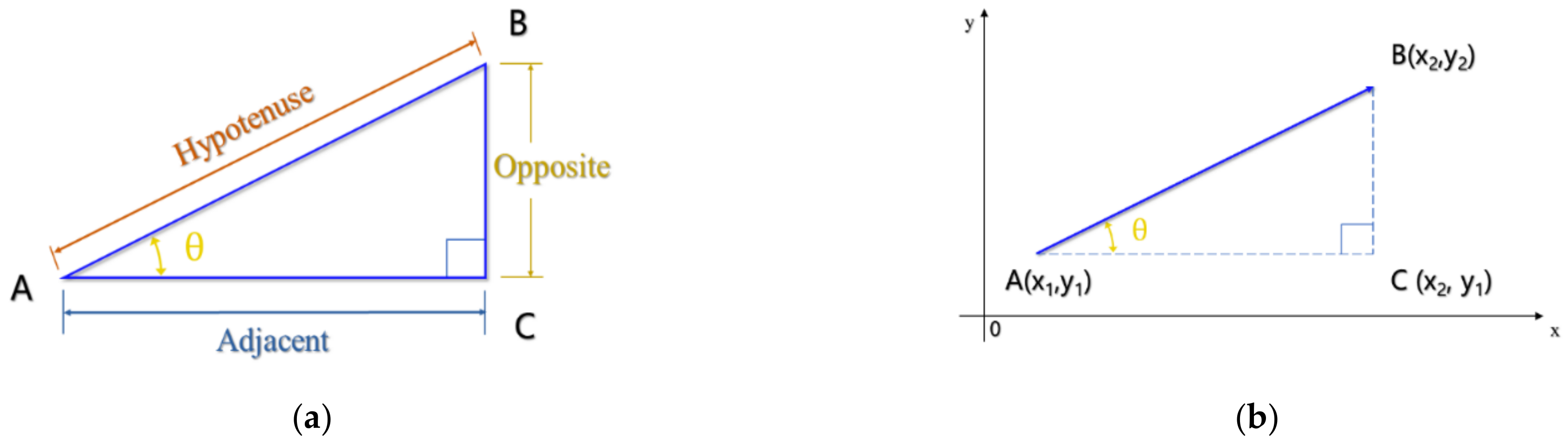
Sine, Cosine, and Tangent are the main functions used in Trigonometry, and they are simply one side of a right-angled triangle divided by another. In Figure 1a, the tangent of θ is the ratio of the opposite to the adjacent, which ranges from negative infinity to positive infinity. When it is 0, the opposite has a zero length and the length of the hypotenuse is equal to that of the adjacent, and the triangle becomes a line segment parallel to the x-axis. In the Plane Rectangular Coordinate System, the direction along the axis is defined as the positive direction. Any directed line segment ( and ) can form a right-angled triangle (Figure 1b), and the slope of is the tangent of θ, that is, . When and , the slope does not exist or it is infinity; and when and , the slope is 0.
In this paper, two directed line segments with the same slope are defined as slope-similar line segments. Particularly, any two line segments parallel to the Y-axis have the same slope. For two line segments with the same slope, whether the directions are congruent or not is determined as follows:
where and are the variations of the two line segments in the X-axis direction, and similarly and are their variations in the Y-axis direction.
Three types of shapes are considered in this study. Slope-similar shapes are defined as two shapes having the same number (at least two) of slope-similar line segments with the consistent (same or opposite) direction. Further, the slope-similar shapes are congruent shapes if the corresponding line segments have the same length, and the congruent shapes are same shapes if the points of the corresponding line segments are in the same position. As the definition suggests, the latter is a special case of the former. The shape comparison of each type is shown in Table 1.
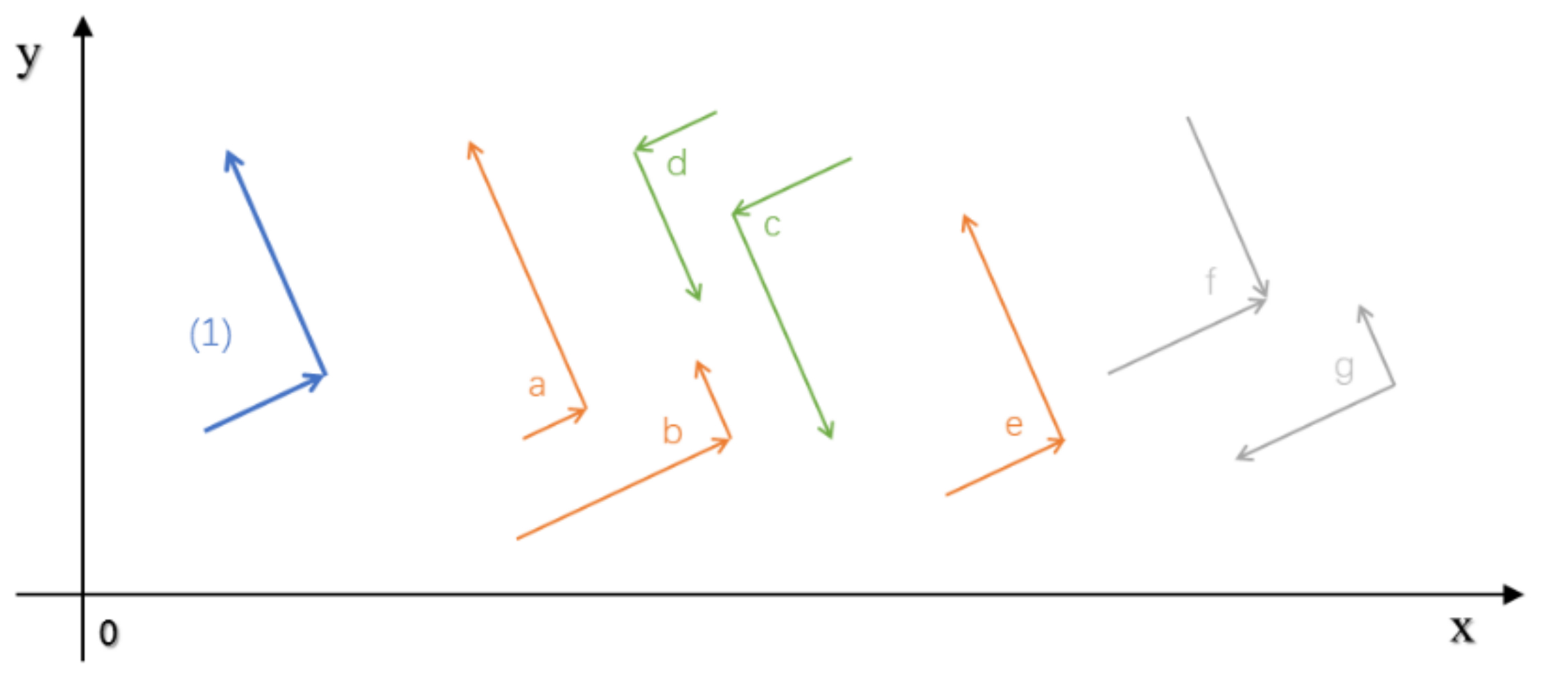
The three types of shapes are further illustrated using a shape consisting of two-line segments (Figure 2 (1)). The slopes of shapes a–e are the same as that of shape (1), and the lengths of the line segments of shapes c/e are also the same as that of shape (1). According to the above definition, neither shape f nor shape g is slope-similar to shape (1). The relationship between other shapes and shape (1) is shown in Table 2.
It is seen that shapes c and e are centrosymmetric shapes.
2.2. Shape Matrix
In Figure 1b, when AC = BC = 1, the triangle is a unit slope similarity base, based on which other line segments can be generated by some rules. The rules can be represented by the following matrix:
where is the ith line segment; or is the starting point position of the unit slope-similar base; and are the scaling multipliers of the unit slope similarity basis in the parallel X-axis and Y-axis directions, respectively, , . By default, = = 1 and the end of the ith line segment is the start of the (I + 1)th line segment. Through the matrix, the coordinates of the end point are ( + , + ), and the slope of the line segment is ( 0). If = 0, the length of the line segment is .
Therefore, two shapes with v line segments can be represented by the following shape matrix:
Conversely, the shape matrix is known when the coordinates of all the shape points and the order of their connections are known.
2.3. Similarity Measures
Based on the definition of the slope-similar shapes, the maximum deviation and the cumulative deviation are two dimensions of indicators to calculate the similarity of two shapes. Different types of shapes require different similarity metrics to be calculated. The details are shown in Table 3.
For the two shapes in shape matrix (3), the formula for calculating the similarity of each index is shown in Table 4.
In order to be applicable to real-world scenarios, the two shapes are said to have the same slope if the difference between the two slopes is less than 0.01. Additionally, thresholds or constraints are introduced to filter target shapes. For example, when the maximum deviation is less than 0.05 and the cumulative deviation is less than 1, the two shapes are slope-similar shapes. It is an ideal or special case when both the maximum deviation and the cumulative deviation are 0. In general, the smaller the values of maximum deviation and cumulative deviation are, the more similar the two shapes will be.
3. Study Area and Methods
3.1. Study Area
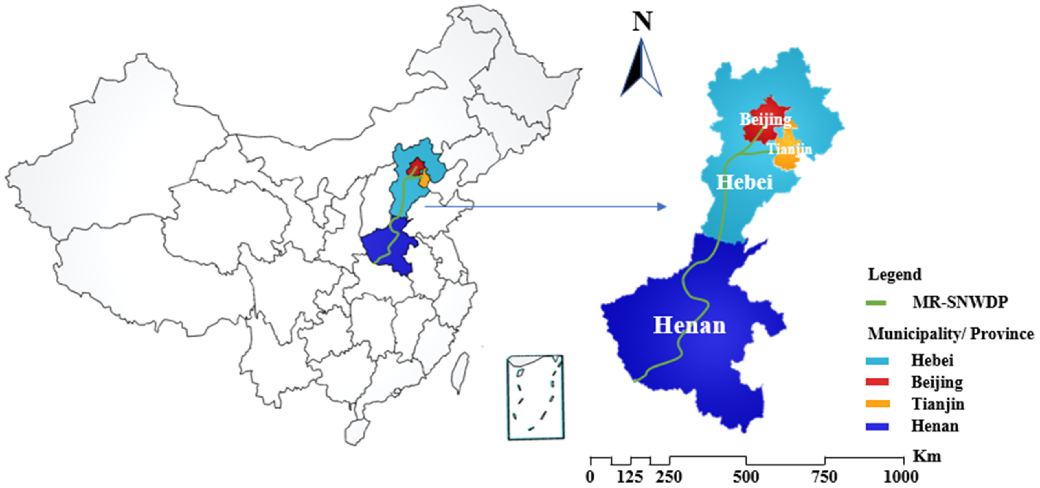
Although China is rich in freshwater resources, the amount of available freshwater resources per capita is very low due to the large population [20]. What makes the situation worse is that water resources are more abundant in the south than in the north [21]. To solve this problem, China has built the world’s largest inter-basin water transfer project, the South-to-North Water Diversion Project (SNWDP). Water is transferred from the Yangtze River and its major tributaries to Beijing and Tianjin, as well as other water users in Shandong, Jiangsu, Hebei, Henan, and Anhui provinces since 2013 (East Line) and 2014 (Middle Line) [22]. As shown in Figure 3 (drawn by NB Map (nbcharts.com)), the Middle Route of SNWDP is intended to divert water from Danjiangkou Reservoir in Hubei Province to Beijing, Tianjin, and other regions. There are more than 60 sluice gates along the 1432 km route. Given the strong coupling of cascaded channels, it is difficult to ensure the water levels of all gates along the route are stable. The water level variation should be controlled within 15 cm per hour and 30 cm per 24 h. There are no lakes and reservoirs for storage of water along the route, which highlights the importance of safe operation, especially during flow adjustment or heavy rainfall periods. Exceeding of the water level threshold may lead to disastrous consequences such as overflow and channel damage. Therefore, real-time water level prediction considering gate opening and flow variation is of great importance for the safety of the project.
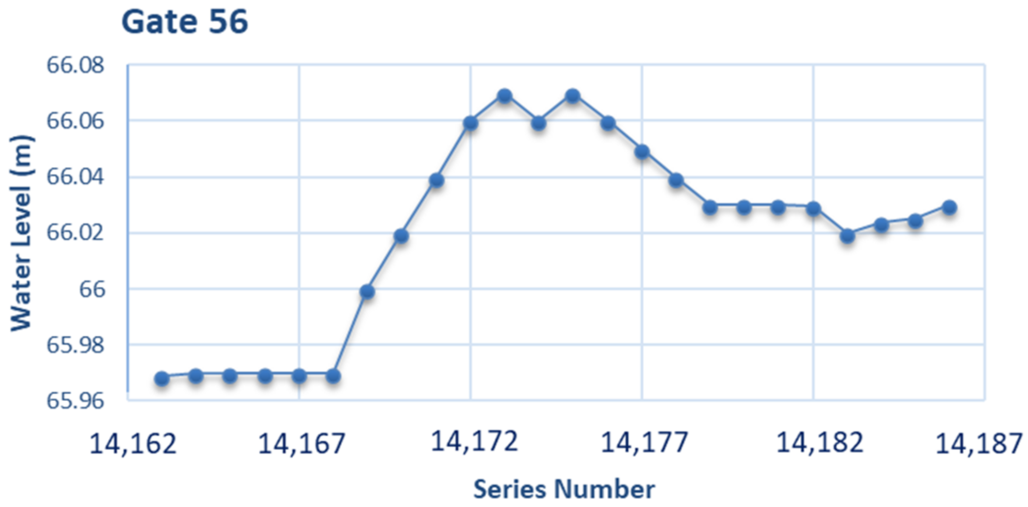
The Middle Route of SNWDP has been operating safely for nearly seven years since its operation in 2014, and its hydrodynamic features such as water levels before sluice gates, gate opening, and flow rates are recorded under various weather and operating conditions. In this study, 15,570 rows of datasets (1 October 2017–28 April 2021) are collected for each gate at 2-h time intervals. Table 5 shows the water level datasets before gate 56 on 1–2 January 2021, and the corresponding trend shape is shown in Figure 4 (drawn by Excel 2021).
Figure 4 shows that (1) the horizontal distances between adjacent data points are 1 (representing a 2-h time interval); (2) the slope of each line segment is , i.e., the water level of the current moment minus that of the previous moment (same as below). When > 0, the slope is greater than 0. When = 0, the slope is equal to 0. When < 0, the slope is less than 0; and (3) the start of the next line segment is the end of the current line segment.
Thus, Equation (2) can be written in the following form:
where is the ith water level data point, and others are the same as above.
The water level variation is retained to the centimeter level with a minimum variation of 0.01 m. The shape matrix of Figure 4 is described as follows:
For the Middle Route of SNWDP, the water level change before each gate is usually required to be less than 0.06 m, which is achieved by precisely controlling the gates between two adjacent open channels. Taking the water level before gates 3, 4, 5, 6, and 7 as an example, the results of water level change () at adjacent moments of each gate are shown in Table 6.
Here, water level changes are divided into the following four categories: A, ; B, ; C, ; D, . As seen in Table 6, more than 99% of water level differences fall into class A, which indicates a relatively stable operation of the project and the ubiquity of slope-similar shapes.
For an open channel consisting of upstream and downstream gates, the working conditions can be divided into four categories according to the change of gate opening: (1) both upstream and downstream gate openings remain unchanged; (2) upstream gate opening changes and downstream gate opening remains unchanged; (3) upstream gate opening remains unchanged and downstream gate opening changes; (4) both upstream and downstream gate openings change. As this paper is concerned with water level prediction considering downstream gate opening variation, only working conditions (3) and (4) are considered.
3.2. Methods
The subsequence of interest is defined as a query [23]. The longer the length of the query is, the less the slope-similar shapes will be. In order to find more potentially slope-similar shapes, the length of the query is set to 3 and the threshold of the same slope is set to 0.01. That is, when the difference between two slopes is less than or equal to 0.01, the two line segments are said to have slope-similar shapes. Equation (1) is used to determine whether the direction is consistent. The maximum deviation of the slope is 0.01, and the cumulative deviation may be 0, 0.01, or 0.02.
The historical water level dataset before gate 5 was selected as the predicted data points. Assuming that the water level data point of the nth moment is one of the predicted data points, the selected dataset should meet the following requirements:
- (1)
- The water levels at the (n − 3)th, (n − 2)th, and (n – 1)th moments are in a stable state, where the upstream and downstream gate opening is kept constant and the water level variation is within 0.02 m. Then, these three data points form a query. Dataset that is slope-similar to query should also meet the above requirements.
- (2)
- The water level difference () at the nth moment is Class A or B.
- (3)
- The downstream gate opening () at the nth moment changes, while the upstream gate opening () is not required.
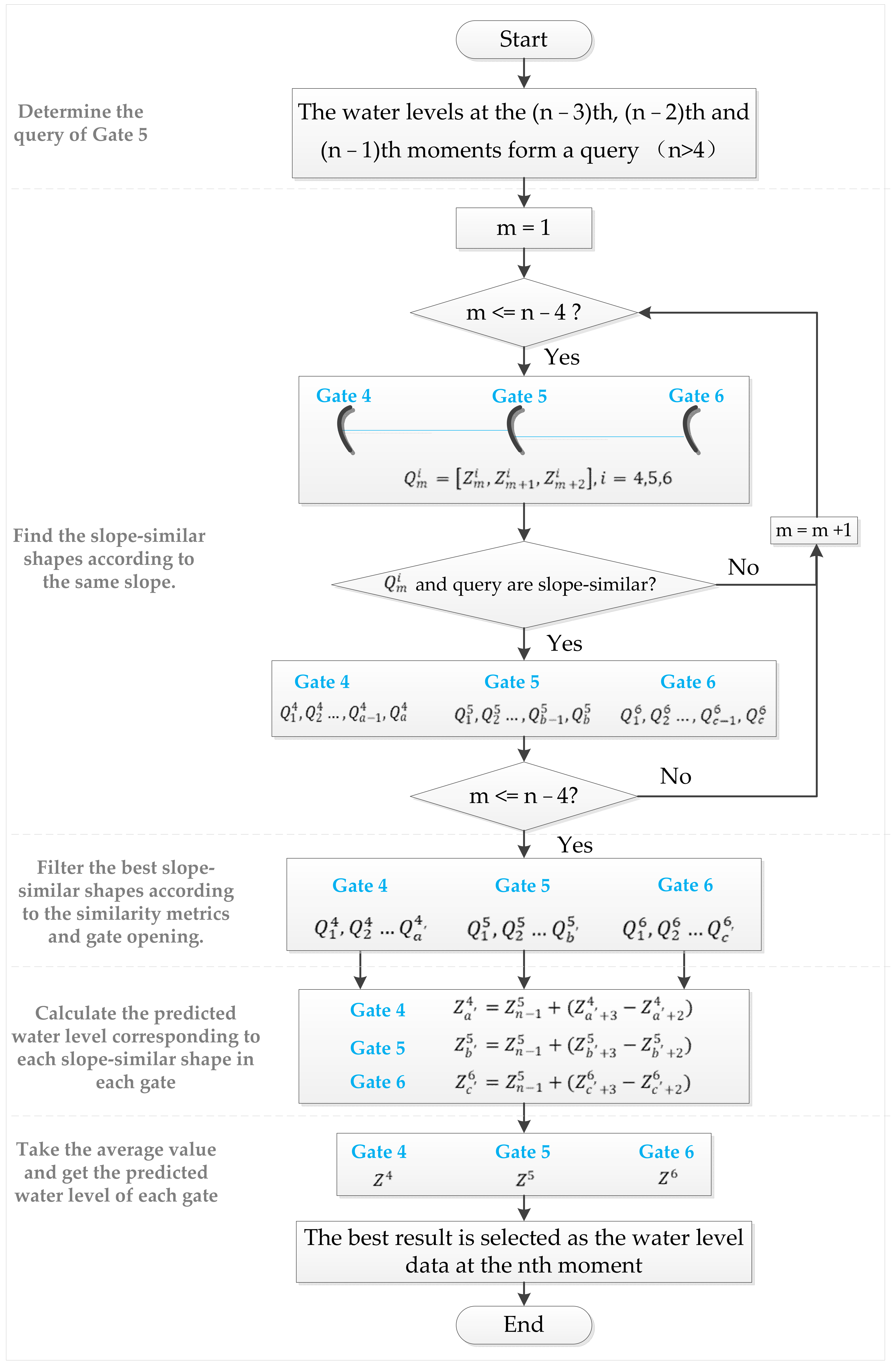
As a similar change trend is expected for water levels of adjacent open channels because of their strong coupling, gates 4 and 6 are used as matching gates. First, historical datasets with water level change trends similar to that of the query are identified by the slope-similar shape method, and then the cumulative deviation and gate opening are used to filter the best slope-similar shapes for each query in the three gates. The water level difference at the next moment (2 h) of the best slope-similar shapes is considered as the water level variation at the next moment of the query (if there is more than one slope-similar shape, the average water level difference is used). Thus, the last water level of the query plus the water level difference is the predicted water level of the query. Finally, for the same query, the best slope-similar shape of each gate is compared horizontally based on the cumulative deviation and gate opening, and the best result is selected as the predicted water level. For the specific query, the water level prediction flowchart is shown in Figure 5 (drawn by Visio 2010).
4. Result and Discussion
The manual selection yields only seven queries that meet all the requirements in Class B of gate 5, and eight queries with representative water level differences are selected in Class A (Table 7). The number of slope-similar shapes (SSS) matched by each query in each gate and the number of best slope-similar shapes (BSSS) after filtering are shown in Table 8. The preliminary results of each query in each gate are shown in Table 9, and the final predicted water level and error of each query are shown in Table 10.
The and in Table 7 show that the change trend of water levels before the downstream gate is usually opposite to that of the downstream gate opening. Additionally, there is no obvious pattern between the change amplitude of water levels before the gate and gate opening. The fourth query causes a drop in water level due to the large drop in flow in previous open channels. However, the flow as an important factor affecting water level is not considered in this paper. The water level fluctuates greatly under steady state conditions and shows no obvious similarity, and unavailability of rainfall and seepage information can lead to large errors in the inflow and outflow of the open channel.
Table 8 reveals that the overall number of SSS in gate 5 is larger than that in gate 4 by 600–1200, while the overall number in gate 4 is larger than that in gate 6 by 130–350. The water level change of the query should be within 0.02 m (i.e., is 0, 0.01 m or 0.02 m). Table 6 reveals that the number of in gate 4 is close to that in gate 6, but both of them are higher than that of gate 5. Therefore, it is concluded that the closer the number of , the closer the number of slope-similar shapes. This provides a basis for selecting appropriate gates. The number of BSSS is only one in most circumstances, indicating that it is necessary to expand the range of same slope. This is acceptable considering monitoring errors, water level fluctuations and other uncertainties.
As the water transfer process is highly stable in the Middle Route of SNWDP, the water level difference at the next moment for each BSSS of the gates is close to zero (Table 9), which in turn leads to larger prediction errors of Class B data points (1st–7th) but smaller prediction errors of Class A data points (8th–15th). It is seen in Table 10 that only two Class B data points have an error less than 0.03; while out of eight Class A data, seven (87.5%) have an error less than 0.03, 71.4% of which have an error less than 0.02. Although there are only eight Class A data points, the proposed slope-similar shape method is feasible and effective because the of the selected Class A data points is representative and there are far more Class A data points than Class B data points. The prediction ability and accuracy of the slope-similar shape method are independent of the project type but directly related to the variation of historical water level data. If 99% of the changes of historical water level data in this case are in the range of 0.05~0.1 m, the prediction accuracy of the method for B class data would be higher than that for A class data.
Our results are encouraging relative to previous results. A multilayer perceptron and recurrent neural network were constructed for real-time water level prediction in the Middle Route of SNWDP, and the accuracy of model prediction deviation within 1 cm, 2 cm, and 3 cm reached 81.36%, 94.09%, and 97.05%, respectively [3]. The high prediction accuracy is due to the small variation (within 5 cm) of the water level data on the one hand and the use of the training data derived from the data under the unchanged gate opening on the other hand. In our study, the difficulty of the prediction is increased, i.e., the real-time prediction under the gate opening at the next moment is considered. The proposed method is interpretable and the results are satisfactory. The study has important implications for the development of steady-state regulation schemes.
Some limitations of this paper are worth mentioning: (1) as the proposed method requires the collection of historical datasets over a long period of time under various conditions, it may not be suitable for newly built open-channel water transfer projects; (2) as there are high requirements for query selection and non-stationary conditions are not considered, it is less applicable to real-time rolling prediction; (3) the monitoring frequency is low that could not fully reflect the water level change under some conditions, resulting in misdiagnosis of water level data. The water level prediction can also be affected by single data source and water level outliers.
5. Conclusions
In this paper, the idea of time series similarity is introduced for the first time for water level prediction of an open-channel water transfer project, and then the novel slope-similar shape method is proposed to characterize water level changes. The method uses the water level data points of three consecutive moments to find the historical water level datasets with similar change trends and the best similar data points according to the similarity index and the change of gate opening at the prediction moment. The water level difference at the next moment of the best similar data points can be used as the water level difference at the prediction moment, and thus the water level at the next moment can be obtained. The method is applied to the Middle Route of SNWDP. The results show that 87.5% of Class A datasets have an error less than 0.03, 71.4% of which have an error less than 0.02. In conclusion, the proposed novel method is feasible, effective, and interpretable, and the study has important implications for the development of scheduling scheme. Future research will focus on real-time water level prediction under non-stationary conditions based on the slope-similar shape, and hydrodynamic models are to be established for water level prediction under extreme conditions.
Author Contributions
Conceptualization, L.Z. and X.L.; methodology, L.Z. and Z.Z.; validation, W.Z., L.Z. and K.A.; data curation, L.Z.; writing—original draft preparation, L.Z.; writing—review and editing, L.Z. Funding Acquisition, W.Z., K.A. and M.H. All authors have read and agreed to the published version of the manuscript.
Funding
This research was supported by Key R&D Program of the China Huaneng Group Co., Ltd. [HNKJ20-H26]; and Water Resources Research Institute of Shandong Province (SDSKYZX202107).
Data Availability Statement
Data available on request due to restrictions, e.g., privacy. The data presented in this study are available from the corresponding author by request ([email protected]).
Conflicts of Interest
The authors declare no conflict of interest.
References
- Han, H.; Wang, Z.; Liu, B. Tournament incentive mechanisms based on fairness preference in large-scale water diversion projects. J. Clean. Prod. 2020, 265, 121861. [Google Scholar] [CrossRef]
- Liu, J.; Li, M.; Wu, M.; Luan, X.; Wang, W.; Yu, Z. Influences of the south–to-north water diversion project and virtual water flows on regional water resources considering both water quantity and quality. J. Clean Prod. 2020, 244, 118920. [Google Scholar] [CrossRef]
- Ren, T.; Liu, X.; Niu, J.; Lei, X.; Zhang, Z. Real-time water level prediction of cascaded channels based on multilayer perception and recurrent neural network. J. Hydrol. 2020, 585, 124783. [Google Scholar] [CrossRef]
- Liu, Y.; Wang, H.; Lei, X.; Wang, H. Real-time forecasting of river water level in urban based on radar rainfall: A case study in Fuzhou City. J. Hydrol. 2021, 603, 126820. [Google Scholar] [CrossRef]
- Liu, Y.; Wang, H.; Feng, W.; Huang, H. Short Term Real-Time Rolling Forecast of Urban River Water Levels Based on LSTM: A Case Study in Fuzhou City, China. Int. J. Environ. Res. Public Health 2021, 18, 9287. [Google Scholar] [CrossRef]
- Berkhahn, S.; Fuchs, L.; Neuweiler, I. An ensemble neural network model for real-time prediction of urban floods. J. Hydrol. 2019, 575, 743–754. [Google Scholar] [CrossRef]
- Guo, T.; He, W.; Jiang, Z.; Chu, X.; Malekian, R.; Li, Z. An Improved LSSVM Model for Intelligent Prediction of the Daily Water Level. Energies 2019, 12, 112. [Google Scholar] [CrossRef] [Green Version]
- Li, B.; Yang, G.; Wan, R.; Dai, X.; Zhang, Y. Comparison of random forests and other statistical methods for the prediction of lake water level: A case study of the Poyang Lake in China. Hydrol. Res. 2016, 47, 69–83. [Google Scholar] [CrossRef] [Green Version]
- Shiri, J.; Shamshirband, S.; Kisi, O.; Karimi, S.; Bateni, S.M.; Hosseini Nezhad, S.H.; Hashemi, A. Prediction of Water-Level in the Urmia Lake Using the Extreme Learning Machine Approach. Water Resour. Manag. 2016, 30, 5217–5229. [Google Scholar] [CrossRef]
- Basu, B.; Morrissey, P.; Gill, L.W. Application of nonlinear time series and machine learning algorithms for forecasting groundwater flooding in a lowland karst area. Water Resour. Res. 2022, 58, e2021WR029576. [Google Scholar] [CrossRef]
- Kim, D.; Lee, J.; Kim, J.; Lee, M.; Wang, W.; Kim, H.S. Comparative analysis of long short-term memory and storage function model for flood water level forecasting of bokha stream in namhan river, korea. J. Hydrol. 2022, 606, 127415. [Google Scholar] [CrossRef]
- Ming, X.; Liang, Q.; Xia, X.; Li, D.; Fowler, H.J. Real-time flood forecasting based on a high-performance 2-d hydrodynamic model and numerical weather predictions. Water Resour. Res. 2020, 56, e2019WR025583. [Google Scholar] [CrossRef]
- Piadeh, F.; Behzadian, K.; Alani, A.M. A critical review of real-time modelling of flood forecasting in urban drainage systems. J. Hydrol. 2022, 607, 127476. [Google Scholar] [CrossRef]
- Wu, R.-S.; Sin, Y.-Y.; Wang, J.-X.; Lin, Y.-W.; Wu, H.-C.; Sukmara, R.B.; Indawati, L.; Hussain, F. Real-time flood warning system application. Water 2022, 14, 1866. [Google Scholar] [CrossRef]
- Bathaee, Y. The artificial intelligence black box and the failure of intent and causation. Harv. J. Law Technol. 2018, 31, 889. [Google Scholar]
- Faloutsos, C.; Ranganathan, M.; Manolopoulos, Y. Fast subsequence matching in time-series databases. In Proceedings of the 1994 ACM SIGMOD International Conference on Management of Data, Minneapolis, MN, USA, 24–27 May 1994; Association for Computing Machinery: Minneapolis, MN, USA, 1994; pp. 419–429. [Google Scholar]
- Keogh, E.J.; Chakrabarti, K.; Pazzani, M.J.; Mehrotra, S.J.K.; Systems, I. Dimensionality Reduction for Fast Similarity Search in Large Time Series Databases. Knowl. Inf. Syst. 2001, 3, 263–286. [Google Scholar] [CrossRef]
- Dong, X.; Gu, C.; Wang, Z. Research on Shape-Based Time Series Similarity Measure. In Proceedings of the 2006 International Conference on Machine Learning and Cybernetics, Dalian, China, 13–16 August 2006; pp. 1253–1258.18. [Google Scholar]
- Wang, D. Pattern distance of time series. WIT Trans. Inf. Commun. Technol. 2003, 29, 10. [Google Scholar] [CrossRef]
- Gao, Y.; Yu, M. Assessment of the economic impact of South-to-North Water Diversion Project on industrial sectors in Beijing. J. Econ. Struct. 2018, 7, 4. [Google Scholar] [CrossRef] [Green Version]
- Geng, S.; Zhou, Y.; Zhang, M.; Smallwood, K.S. A Sustainable Agro-ecological Solution to Water Shortage in the North China Plain (Huabei Plain). J. Environ. Plan. Manag. 2001, 44, 345–355. [Google Scholar] [CrossRef]
- Rogers, S.; Chen, D.; Jiang, H.; Rutherfurd, I.; Wang, M.; Webber, M.; Crow-Miller, B.; Barnett, J.; Finlayson, B.; Jiang, M.; et al. An integrated assessment of China’s South—North Water Transfer Project. Geogr. Res. 2020, 58, 49–63. [Google Scholar] [CrossRef]
- Gogolou, A.; Tsandilas, T.; Palpanas, T.; Bezerianos, A. Comparing Similarity Perception in Time Series Visualizations. IEEE Trans. Vis. Comput. Graph. 2019, 25, 523–533. [Google Scholar] [CrossRef] [PubMed] [Green Version]
Figure 1.
Right-angled triangle and its sides (a); right-angled triangle by directed line segment (b).
Figure 1.
Right-angled triangle and its sides (a); right-angled triangle by directed line segment (b).

Figure 2.
Shapes formed by two line segments.

Figure 3.
The map of the Middle Route of the South-to-North Water Diversion Project.

Figure 4.
The change trend of water levels before gate 56.

Figure 5.
Water level prediction flowchart. It should be noted that query is selected in this paper to verify the effectiveness of the proposed method, but it is always the three consecutive water level data points at the latest moment in actual water level prediction. is the water level data at the mth moment in the ith gate; is the dataset consisting of the water level at moment m, m + 1, and m + 2 in the ith gate. a, b, and c are the number of slope-similar shapes in gates 4, 5, and 6, respectively, and after filtering, the numbers are a′, b′, and c′, respectively. For gate 5, is the query when m = n − 3, so it needs to be skipped. Python 3.9 is used to search for slope-similar shapes for each gate and to filter the best slope-similar shapes.


Table 1.
Comparison of the three types of shapes.
| Shape Type | Same Slope | Congruent Direction | Same Length | Same Point Position |
|---|---|---|---|---|
| Slope-Similar Shapes | √ 1 | √ | ||
| Congruent Shapes | √ | √ | √ | |
| Same Shapes | √ | √ | √ | √ |
1 It is same for corresponding line segments of that type of shape.
Table 2.
Relationship of shapes a–e to shape (1).
| Relation to Shape (1) | Congruent Direction | |
|---|---|---|
| Same | Opposite | |
| Slope-similar shapes | a/b/e | c/d |
| Congruent shapes | e | c |
| Same shapes | (1) | None |
Table 3.
Similarity metrics for different types of shapes.
| Shape Type | Maximum Deviation | Cumulative Deviation |
|---|---|---|
| Slope-similar shapes | slope | slope |
| Congruent shapes | slope/length | slope/length |
| Same shapes | slope/length/point position | slope/length/point position |
Table 4.
The formula for calculating the similarity of each index.
| Dimensions and Metrics | Slope | Length | Point Position |
|---|---|---|---|
| Maximum deviation | 1 | ||
| Cumulative deviation |
1 when
and , , and vice versa.
Table 5.
The water level datasets before gate 56 with hydrodynamic features.
| No. | Date and Time | Water Level before the Gate (m) | Gate-Hole 1 (mm) | Gate-Hole 2 (mm) | Flow (m3/s) | Outlet 1 (m3/s) | Outlet 2 (m3/s) |
|---|---|---|---|---|---|---|---|
| 4 | 2017-*-* 00:00:00 | 144.5588 | 1800 | 1800 | 174.3318 | 01 | 0 |
| 4 | 2017-*-* 02:00:00 | 144.5545 | 1800 | 1800 | 176.2681 | 0 | 0 |
| 4 | ……… | … | … | … | … | … | … |
| 4 | 2018-*-* 00:00:00 | 144.6506 | 1280 | 1280 | 142.9575 | 0 | 0 |
| 4 | ……… | … | … | … | … | … | … |
| 4 | 2021-*-* 18:00:00 | 144.6653 | 4260 | 4260 | 298.6489 | 0 | 0 |
| 4 | 2021-*-* 20:00:00 | 144.6877 | 4260 | 4260 | 301.7434 | 0 | 0 |
Series No.: The data point for each gate is sequentially numbered from 1–15,570 in chronological order. Date and time: The date and time at which data points were recorded. The time interval is 2 h, yielding 12 records per day. Water level before the gate: The water levels were measured by water level meters in a unit of centimeter. The values reported here are the average water levels of all gate holes. Gate-hole1, Gate-hole2: The values represent the opening sizes of each gate hole for each gate, and the number of holes is in a range of 2 to 4 for each gate. The average opening variation of each gate is used. Flow: The flow is the sum of the flow passing through each gate hole. Outlet: Outlets are in the upstream channel of the gate, and the number of outlets varies from channel to channel. In this paper, the data points from all outlets are combined to yield the total outlet.
Table 6.
Water level changes in each gate.
| Gate | Δz = 0 | |Δz| ≤ 0.05 m | |Δz| ≤ 0.1 m | |Δz| ≤ 0.2 m | 0.2 < |Δz| ≤ 2 m |
|---|---|---|---|---|---|
| 3 | 9116 | 6356 | 50 | 14 | 9 |
| 4 | 10,171 | 5318 | 42 | 8 | 6 |
| 5 | 7868 | 7598 | 58 | 17 | 4 |
| 6 | 10,496 | 4974 | 54 | 8 | 3 |
| 7 | 8976 | 6501 | 43 | 13 | 2 |
Each gate has a total of 15,570 water level data points, yielding 15,569 water level differences. Differences greater than 2 m are excluded because they are usually caused by extreme outliers. For each gate, there are only 2~3 sets of water level data points that are all 0 at adjacent moments, which can be ignored.
Table 7.
Queries and corresponding information.
| No. | Query Index | Predicted Data (m) | (m) | (mm) | (mm) | Matching Gates |
|---|---|---|---|---|---|---|
| 1 | 165–167 | 142.8806 | −0.07 | 200 | 280 | 4/5/6 |
| 2 | 2436–2438 | 142.9752 | −0.08 | 240 | 240 | 4/5/6 |
| 3 | 3231–3233 | 142.8062 | 0.06 | −300 | −600 | 4/5/6 |
| 4 | 11,802–11,804 | 143.22 | −0.07 | −2700 | −3275 | 4/5/6 |
| 5 | 12,043–12,045 | 143.3324 | −0.06 | 400 | 400 | 4/5/6 |
| 6 | 12,250–12,252 | 143.1059 | −0.06 | 0 | 150 | 4/5/6 |
| 7 | 12,825–12,827 | 143.12 | 0.06 | −340 | −400 | 4/5/6 |
| 8 | 148–150 | 142.9767 | −0.05 | 250 | 200 | 4/5/6 |
| 9 | 207–209 | 143.0487 | −0.02 | 0 | 40 | 4/5/6 |
| 10 | 476–478 | 143 | 0.04 | −300 | −270 | 4/5/6 |
| 11 | 561–563 | 143.0766 | 0.03 | −90 | −100 | 4/5/6 |
| 12 | 1077–1079 | 142.9208 | 0.02 | 0 | −110 | 4/5/6 |
| 13 | 2152–2154 | 142.9296 | −0.04 | 145 | 150 | 4/5/6 |
| 14 | 2399–2401 | 142.9333 | 0.02 | 0 | −60 | 4/5/6 |
| 15 | 2543–2545 | 142.9209 | −0.03 | 310 | 150 | 4/5/6 |
Table 8.
Number of slope-similar shapes for each query in each gate.
| No. | Gate 4 | Gate 5 | Gate 6 | |||
|---|---|---|---|---|---|---|
| SSS | BSSS | SSS | BSSS | SSS | BSSS | |
| 1 | 2843 | 1 | 3561 | 2 | 2509 | 1 |
| 2 | 695 | 1 | 1382 | 1 | 565 | 1 |
| 3 | 2991 | 1 | 3985 | 2 | 2777 | 2 |
| 4 | 3012 | 0 | 4006 | 0 | 2797 | 0 |
| 5 | 2801 | 1 | 3496 | 1 | 2507 | 1 |
| 6 | 2991 | 1 | 3995 | 1 | 2778 | 2 |
| 7 | 3014 | 1 | 4053 | 1 | 2791 | 1 |
| 8 | 2987 | 1 | 3961 | 2 | 2783 | 1 |
| 9 | 2622 | 1 | 3568 | 1 | 2367 | 2 |
| 10 | 2851 | 1 | 3713 | 1 | 2536 | 1 |
| 11 | 2784 | 1 | 3393 | 1 | 2493 | 1 |
| 12 | 2009 | 1 | 3195 | 1 | 1693 | 2 |
| 13 | 2990 | 2 | 3950 | 1 | 2787 | 1 |
| 14 | 1694 | 1 | 2775 | 1 | 1364 | 1 |
| 15 | 2846 | 1 | 3684 | 2 | 2531 | 1 |
Table 9.
Water level difference and predicted error of BSSS.
| No. | Gate 4 | Gate 5 | Gate 6 | |||
|---|---|---|---|---|---|---|
(m) | Error (m) | (m) | Error (m) | (m) | Error (m) | |
| 1 | 0 | 0.07 | −0.03 | 0.04 | −0.05 | 0.02 |
| 2 | −0.01 | 0.07 | −0.03 | 0.05 | −0.04 | 0.04 |
| 3 | 0.06 | 0 | −0.03 | −0.09 | 0.02 | −0.04 |
| 4 | / | / | / | / | / | / |
| 5 | −0.01 | 0.05 | −0.02 | 0.04 | −0.01 | 0.05 |
| 6 | −0.01 | 0.05 | −0.01 | 0.05 | −0.02 | 0.04 |
| 7 | 0.05 | −0.01 | 0.01 | −0.05 | 0.02 | −0.04 |
| 8 | −0.01 | 0.04 | −0.03 | 0.02 | −0.04 | 0.01 |
| 9 | 0 | 0.02 | −0.01 | 0.01 | −0.01 | 0.01 |
| 10 | −0.02 | −0.06 | 0.01 | −0.03 | 0.01 | −0.03 |
| 11 | −0.02 | −0.05 | 0.01 | −0.02 | 0.01 | −0.02 |
| 12 | 0.02 | 0 | 0.02 | 0 | 0.02 | 0 |
| 13 | −0.01 | 0.03 | −0.02 | 0.02 | −0.02 | 0.02 |
| 14 | 0.02 | 0 | −0.01 | −0.03 | 0.01 | −0.01 |
| 15 | −0.01 | 0.02 | −0.03 | 0 | −0.02 | 0.01 |
Table 10.
Final predicted water level and error for each query.
| No. | Predicted Water Level (m) | Errors (m) | Gate Source | Index | (mm) | (mm) |
|---|---|---|---|---|---|---|
| 1 | 142.9006 | 0.02 | 6 | 151 | 200 | 250 |
| 2 | 143.0252 | 0.05 | 5 | 10,657 | 240 | 260 |
| 3 | 142.8062 | 0 | 4 | 9035 | −600 | −600 |
| 4 | 143.22 | / | / | / | / | / |
| 5 | 143.3824 | 0.05 | 4 | 11,073 | 400 | 400 |
| 6 | 143.1059 | 0.05 | 4 | 8074 | 0 | 150 |
| 7 | 143.08 | −0.04 | 6 | 8865 | −350 | −400 |
| 8 | 142.9867 | 0.01 | 6 | 15,149 | 220 | 200 |
| 9 | 143.0587 | 0.01 | 5 | 8319 | 0 | 40 |
| 10 | 142.97 | −0.03 | 6 | 8675 | −250 | −250 |
| 11 | 143.0566 | −0.02 | 6 | 4483 | −110 | −130 |
| 12 | 142.9208 | 0 | 4 | 8232 | 0 | −130 |
| 13 | 142.9496 | 0.02 | 6 | 12,249 | 150 | 150 |
| 14 | 142.9333 | 0 | 4 | 3258 | 0 | −60 |
| 15 | 142.9309 | 0.01 | 6 | 12,249 | 150 | 150 |
Publisher’s Note: MDPI stays neutral with regard to jurisdictional claims in published maps and institutional affiliations. |
© 2022 by the authors. Licensee MDPI, Basel, Switzerland. This article is an open access article distributed under the terms and conditions of the Creative Commons Attribution (CC BY) license (https://creativecommons.org/licenses/by/4.0/).
Share and Cite
MDPI and ACS Style
Zhou, L.; Zhang, Z.; Zhang, W.; An, K.; Lei, X.; He, M. Real-Time Water Level Prediction in Open Channel Water Transfer Projects Based on Time Series Similarity. Water 2022, 14, 2070. https://doi.org/10.3390/w14132070
AMA Style
Zhou L, Zhang Z, Zhang W, An K, Lei X, He M. Real-Time Water Level Prediction in Open Channel Water Transfer Projects Based on Time Series Similarity. Water. 2022; 14(13):2070. https://doi.org/10.3390/w14132070
Chicago/Turabian StyleZhou, Luyan, Zhao Zhang, Weijie Zhang, Kaijun An, Xiaohui Lei, and Ming He. 2022. "Real-Time Water Level Prediction in Open Channel Water Transfer Projects Based on Time Series Similarity" Water 14, no. 13: 2070. https://doi.org/10.3390/w14132070
Note that from the first issue of 2016, this journal uses article numbers instead of page numbers. See further details here.