Impacts and Implications of Land Use Land Cover Dynamics on Groundwater Recharge and Surface Runoff in East African Watershed

Abstract

Assessing the spatiotemporal dynamics of land use land cover (LULC) change on water resources is vital for watershed sustainability and developing proper management strategies. Evaluating LULC scenarios synergistically with hydrologic modeling affords substantial evidence of factors that govern hydrologic processes. Hence, this study assessed the spatiotemporal effects and implications of LULC dynamics on groundwater recharge and surface runoff in Gilgel Gibe, an East African watershed, using the Soil and Water Assessment Tool (SWAT) model. Three different LULC maps (2000, 2010, and 2020) were derived from Landsat images, and the comparisons pointed out that the land-use pattern had changed significantly. The agricultural land and grassland cover increased by 3.76% and 1.36%, respectively, from 2000 to 2020. The implications acquired for 2000 show that forested land covers decreased by 5.49% in 2020. The SWAT simulation process was executed using a digital elevation model, soil, LULC, and weather data. The model was calibrated and validated using streamflow data to understand the surface runoff and groundwater recharge responses of each Hydrologic Response Units on reference simulation periods using the Calibration and Uncertainty Program (SWAT-CUP), Sequential Uncertainty Fitting (SUFI-2) algorithm. The observed and simulated streamflows were checked for performance indices of coefficient of determination (R²), Nash–Sutcliffe model efficiency (NSE), and percent bias (PBIAS) on monthly time steps. The results show that there is good agreement for all LULC simulations, both calibration and validation periods (R² & NSE ≥ 0.84, −15 < PBIAS < +15). This reveals that for the LULC assessment of any hydrological modeling, the simulation of each reference period should be calibrated to have reasonable outputs. The study indicated that surface runoff has increased while groundwater decreased over the last two decades. The temporal variation revealed that the highest recharge and runoff occurred during the wet seasons. Thus, the study can support maximizing water management strategies and reducing adverse driving environmental forces.

1. Introduction

Land and water resources are dynamically hindered by uncertainties of climate and land use land cover (LULC) changes, aggravating the water crisis worldwide [1,2]. Inappropriate exploitation and poor management systems increasingly threaten land and water resources, changing the natural landscapes for human use [3,4,5]. Examining the possible effects of LULC change on the hydrologic cycle under natural and human activities is required to manage available resources properly [6]. However, LULC change responses to environmental and socio-economic drivers continue to be a significant scientific hindrance in assessing its effect on water availability [7]. In different climate regions, groundwater is the main fresh water supply; its utilization and management are thoroughly associated with the Sustainable Development Goals [8,9,10]. Conversely, in most African countries, the salient use of groundwater for domestic and agricultural purposes significantly affects groundwater recharge and food security [5,8,11].

Human activities incur massive changes in the terrestrial environment, but the possible effects and implications of such changes on groundwater recharge and surface runoff (GRSURQ) are poorly understood. In Africa, the influence of LULC is much larger than climate variability [12]. The spatiotemporal variability of groundwater recharge and streamflow is essential in understanding the abstraction scenarios of water management [13,14]. Groundwater is a preferable water supply over surface water, while the extreme inter-annual rainfall variations stress surface water availability [15]. However, the impacts of LULC change on groundwater recharge are not sufficiently recognized, though it is a substantial freshwater source for domestic, agricultural, and commercial uses, which results in groundwater depletion [16]. The main implications are overexploitation of natural resources [17], ecosystem service [18], erosion, land degradation, and deforestation [19,20], which affect ecological and economic sustainability [21].

In developing countries such as Ethiopia, estimating GRSURQ is challenging because of the scarcity of relevant data [13]. Ethiopia has significant land and water resources, playing a minimum role in developing the national economy. It is being affected by various environmental challenges in order to enhance agricultural productivity for food security. Over the past decades, an extensive LULC change has been observed mainly from manmade and natural forces [22,23]. Both natural and anthropogenic activities adversely affect watershed hydrology, causing water stress, which shifts ecosystem biodiversity. Many studies have assessed drivers of LULC change affecting environmental resources [24]. Of which, cutting of trees for fuelwood and charcoal [25,26], resettlement, land tenure policy, population growth, poverty, intensive agricultural practice [27,28], and drought occurrence [29,30] have been recognized as primary drivers in different parts of the country. Poor LULC practices in highland areas have resulted in substantial soil loss, reduced agricultural production, and groundwater depletion [31]. This adversely affects essential aspects of the environment, geomorphologic patterns, flora and fauna [32], habitat fragmentation, depletion of biodiversity [33], and changes in climatic conditions [34]. Where many drivers can potentially conceal, reducing the impacts of LULC change on groundwater recharge is paramount [35].

LULC change affects spatiotemporal scales of land surfaces, changing surface runoff, groundwater recharge, evapotranspiration, and river flow [36,37,38]. However, critical water stress has been faced due to information gaps in the decision-making process in most developing countries, including Ethiopia [13]. Understanding the hydrologic cycle to establish a suitable model for a watershed is crucial in planning and utilizing water resources. Nevertheless, analyzing and quantifying hydrologic components require a realistic hydrologic model representing watershed processes [39]. Watershed models have been used as a dynamic mechanism to address a comprehensive spectrum of environmental problems, advancing estimates’ predictive accuracy [28,40,41]. The Soil and Water Assessment Tool (SWAT) [42] is a vigorous hydrologic model to estimate hydrologic fluxes in combating water scarcity issues [43,44,45,46]. The model integrates multiple ecological processes supporting management and decision-making scenarios worldwide [39,41,47,48,49,50,51,52,53].

The heterogeneity of variations in hydrological fluxes with LULC change over the years challenges how to realize the possible effects [54]. Qualifying and quantifying the spatiotemporal variations of groundwater recharge based on updated spatial information are indispensable for watershed sustainability [13,55]. Nonetheless, basic information on the spatiotemporal patterns of LULC change and its effect on GRSURQ in Ethiopia is rarely understood, while water and food security are central issues. GRSURQ is challenging because of drastic changes in vast anthropogenic activities. Controlling undesirable surface runoff in watersheds preserves soil nutrients and water availability, maximizing crop yields to reduce food security issues [56]. Furthermore, surface runoff is the driving energy of soil erosion to reservoirs [57], which might result in sediment deposition, directly affecting groundwater recharge if not adequately regulated.

In the Gilgel Gibe watershed, where the surface water is intermittent due to the erratic nature of rainfall, groundwater is becoming a critical source of fresh water, as locating sustainable and productive aquifers is challenging [58]. Hence, modeling efforts in LULC change are fundamental to developing water infrastructure supporting sustainable watershed management strategies in data-sparse environments. Sustainable water resources management requires a significant understanding of the effects and implications of LULC and watershed monitoring strategies. However, no exclusive evidence exists on how changes to LULC affect GRSURQ in the Gilgel Gibe watershed. Thus, the present study aims to assess the spatiotemporal effects and implications of LULC dynamics on groundwater recharge and surface runoff in the Gilgel Gibe watershed, Ethiopia, in East Africa, using the SWAT model over the past two decades. The SWAT model was successfully applied to assess the exclusive effects of LULC changes on GRSURQ to verify the viability of predicting streamflow with independent calibration and validation for each LULC period simulation. This study is robustly helpful in promoting sustainable watershed management and resource development programs under data-scarce conditions. This will enable planners and policy-makers to apply effective management strategies to diminish the undesirable effects of natural and uncontrolled human activities.

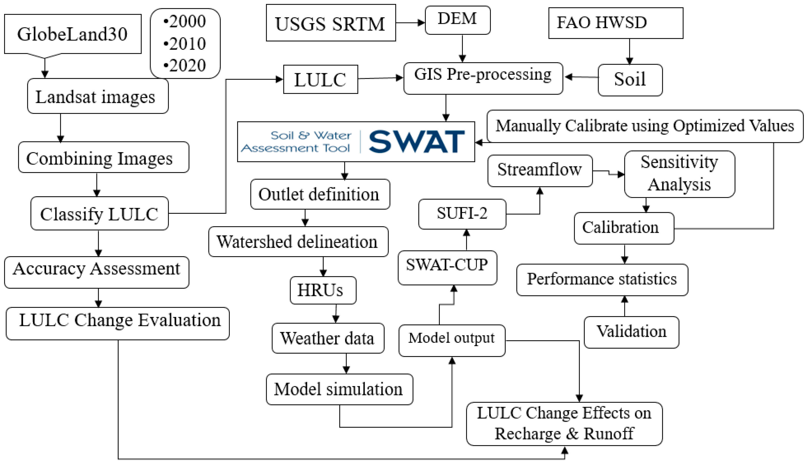
2. Materials and Methods

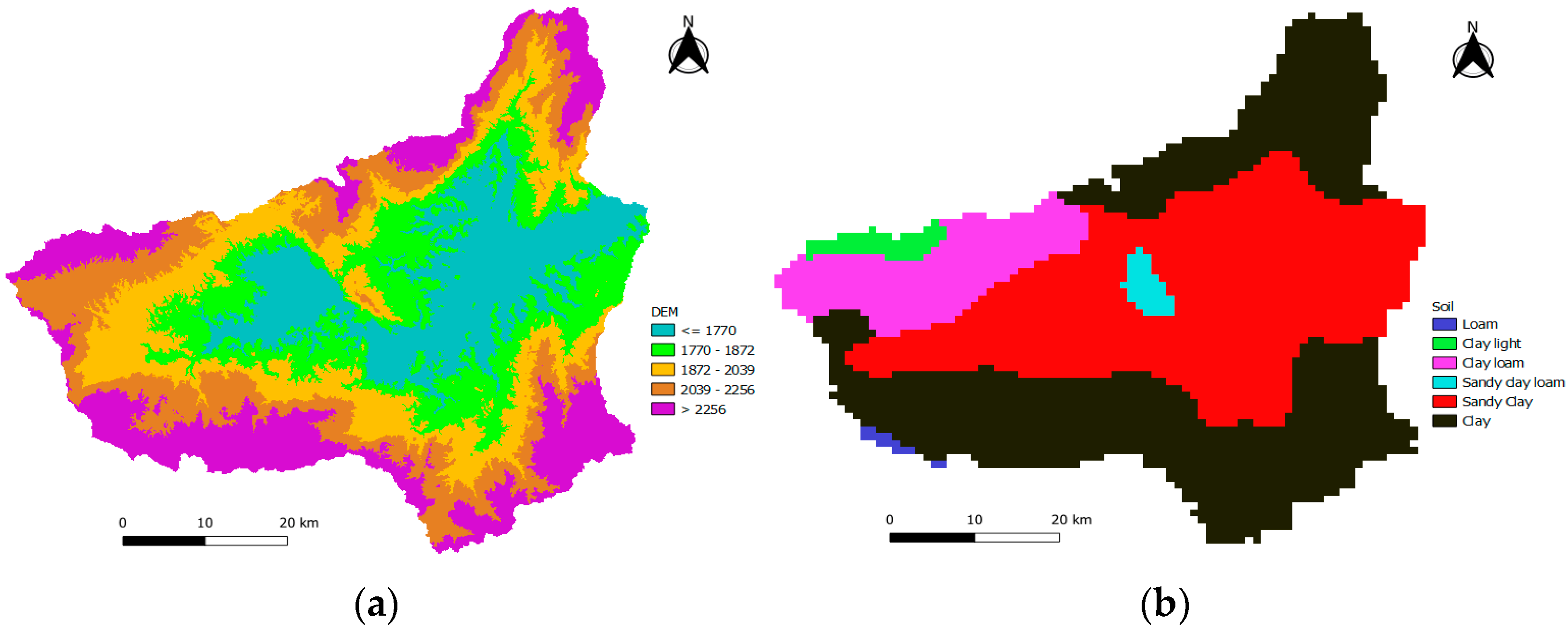
2.1. Description of Study Area

The Gilgel Gibe watershed is situated in Eastern Africa, the Omo-Gibe River Basin, and a semi-arid southwestern region of Ethiopia. The watershed reaches through the Addis Ababa–Jimma–Gambella asphalt road to the west of the Main Ethiopian Rift. The dominant soil types are alisols (45.11%), vertisols (40.79%), nitisols (13.73%), and leptosols (0.37%), with textures ranging from clay to sandy loam [58]. The areal coverage of slope in percentage is 0–5 (15.41%), 5–10 (15.63%), 10–15 (16.55%), 15–35 (40.75%), and 11.65% for slopes above 35 degrees [58]. The geological structures are columnar joints in basalts and flow bands in trachytes and rhyolites. The area reveals Tertiary volcanic rocks, Precambrian basements, Mesozoic rocks, Pliocene age volcanics, quaternary pyroclastics, and alluvial sediments [59].

2.2. SWAT Model Description

The Soil and Water Assessment Tool (SWAT) [42] is a continuous, physically based, and lumped model capable of simulating water management environments [45,60]. The model is developed to simulate runoff and nutrient losses with readily available input data to assess management practices [42,61]. SWAT has usually been used to evaluate the impacts and implications of LULC change on watershed hydrology [17,23,36,48,62]. It simulates a shallow unconfined aquifer that donates water to the mainstream or reaches the sub-basin and a confined deep aquifer [61]. This enhances the precision of the water balance, providing robust physical meaning. In addition, SWAT simulates the hydrological cycle [43,63] using the water balance Equation (1).

$$S{W}_t=S{W}_o+{{\displaystyle \sum }}_{i=1}^t\left(R_{day}-Q_{surf}-E_a-W_{seep}-Q_{gw}\right)$$

(1)

where: SW_t final water content (mmH₂O), SW_o initial soil water content (mmH₂O), t time (days), Rday precipitation amount (mmH₂O), $Q_{surf}$ surface runoff (mmH₂O), E_a actual evapotranspiration (mmH₂O), Wseep water entering vadose zone from soil profile (mmH₂O), Q_gw return flow amount (mmH₂O).

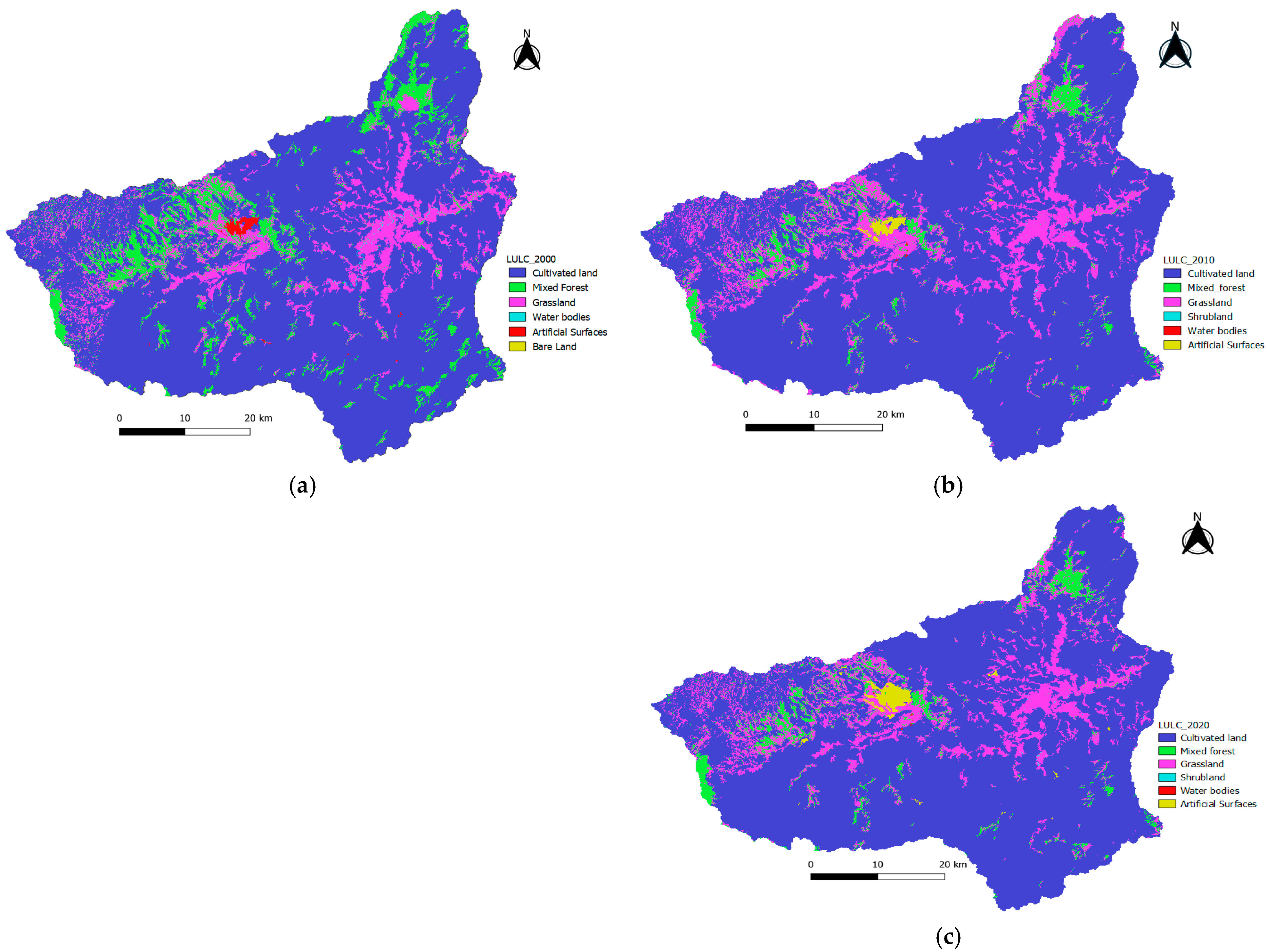
2.3. Model Input Data Preparation

The SWAT model needs topography, LULC, soil, and daily weather data to simulate hydrologic processes. Digital elevation model (DEM) represents watershed topography attained from the Shuttle Radar Topography Mission of the US Geological Survey (Figure 1a). The soil data were acquired from Food and Agriculture Organization (FAO), Harmonized World Soil Database (HWSD) [64]. HWSD Viewer Version 1.21 [65] was used to generate a code for soil properties. Different types of soil texture and physical-chemical properties of soils are required for SWAT simulations [61,66]. The dominant soil groups were identified, the soil map was attached to the soil database (Figure 1b), and a lookup table was prepared that links the soil class and input soil map to the SWAT model database.

LULC data were retrieved from accurate and high-resolution Landsat images [67], Global Land Cover Datasets of GlobeLand30 [68]. This study considered LULC of the years 2000 (Figure 2a), 2010 (Figure 2b), and 2020 (Figure 2c). LULC accuracy assessment was executed using Semi-Automatic Classification Plugin (SCP) for the Quantum Geographic Information System (QGIS) environment. It was accomplished by comparing a sample of points (ground truth) to assess the dependability and precision of the classified map. A confusion matrix was used to categorize the accuracy derived from the user’s accuracy, producer’s accuracy, and the kappa information. A kappa distribution rate of more than zero is considered to be good agreement [69]. Kappa coefficient measures how the classification results compare to values assigned randomly. If the kappa coefficient equals one, the classified and ground truth images are identical. Finally, the accuracy of LULC maps was checked to gain confidence for test applications.

The GlobeLand30 Classification System has specifically given details for each LULC type. Cultivated land (AGRC) is used to produce crops; it comprises irrigated upland, vegetable land, cultivated pasture, and coffee garden. Forest (FRST) is land covered with trees, mixed forests, and sparse woodland, occupying a maximum density of over 30%. Grassland (RNGE) is land protected by natural grass with a cover density of over 10%. Shrubland (SHRB) is the land covered with shrubs, and the cover density is over 30%. Wetland (WETN) denotes the junction of land and water areas covered by hygrophyte and wet soils. In contrast, water bodies (WATR) refer to the area’s liquid water-covered river, reservoirs, and pit-pond. Artificial surfaces (URBN) denote surfaces made by man-built activities in urban and rural areas and industrial and transportation facilities. Bare land (RNGB) includes naturally covered lands such as desert, sand, gravel ground, bare rocks, saline, and alkaline lands with a cover density lower than 10%. SWAT uses these codes to link the LULC of the study watershed to the SWAT land use database. Subsequently, a user lookup table was prepared that identifies SWAT code (AGRC, FRST, RNGE, SHRB, WATR, URBN, and RNGB) for each LULC category to simulate the model. Finally, each LULC (2000, 2010, and 2020) period map was used for a separate SWAT model (1988–2018) simulation of hydrologic processes.

2.4. SWAT Model Setup and Simulation

SWAT model setup was developed to simulate the watershed hydrological process and evaluate GRSURQ. First, the stream definition was carefully determined by selecting the threshold required to form the origin of streams. In this present study, the slope map was produced from DEM data. The study established the multiple slope option, considering different slope classes to create hydrologic response units (HRUs). Then, the land area was distributed into HRUs with exclusive evidence related to various features of land use, management, and soil attributes [61,70]. HRUs are defined in the QSWAT [71] interface of the QGIS environment. QSWAT is written in a robust programming language, Python, with anticipated supporting code readability [71]. HRUs increase accuracy in predicting loadings from the sub-basin. The LULC and soil data are used to delimit HRUs and tie the DEM with the crop and soil databases. A 5–10% threshold value is used to avoid small HRUs, reduce the total number of HRUs, and increase model efficiency [61]. All soil water balance constituents are computed on an HRU basis as comparable HRUs would have analogous hydrologic features [42].

Weather data definition is an essential requirement for SWAT simulation. The SWAT 2012 requires daily precipitation (mm), temperature (°C), relative humidity (percentage), solar radiation (MJ/m²), and wind speed (m/s) of meteorological stations inside and in the buffer zone of the watershed. The present study used Jimma, Sekoru, Shebe, Assendabo, Busa, Dedo, and Omo Nada weather stations collected from the National Meteorological Agency to simulate the hydrology of the watershed. The streamflow data were collected from the Ministry of Water, Irrigation, and Electricity. Weather Generator (WGN) Parameters Estimation Tool interpolates missing data from the synoptic stations for specific simulation periods. Hence, WGN provided all necessary statistical information of synthetic daily meteorological records to fill in missing data appropriately. WGN generates wind speed, solar radiation, and relative humidity from precipitation and temperature [61]. After computing the WGN parameter, the corresponding lookup table was prepared according to the SWAT model format, including the two-year warmup periods. The warmup period was taken to ensure no effects from the initial conditions. Then, the LULC, soil, and slope layers were overlaid, basin-wise HRUs were created, weather data were defined, and SWAT2012 was simulated with the total simulation period from 1988 to 2018. The general outline of the workflow structure used in this assessment is shown in Figure 3.

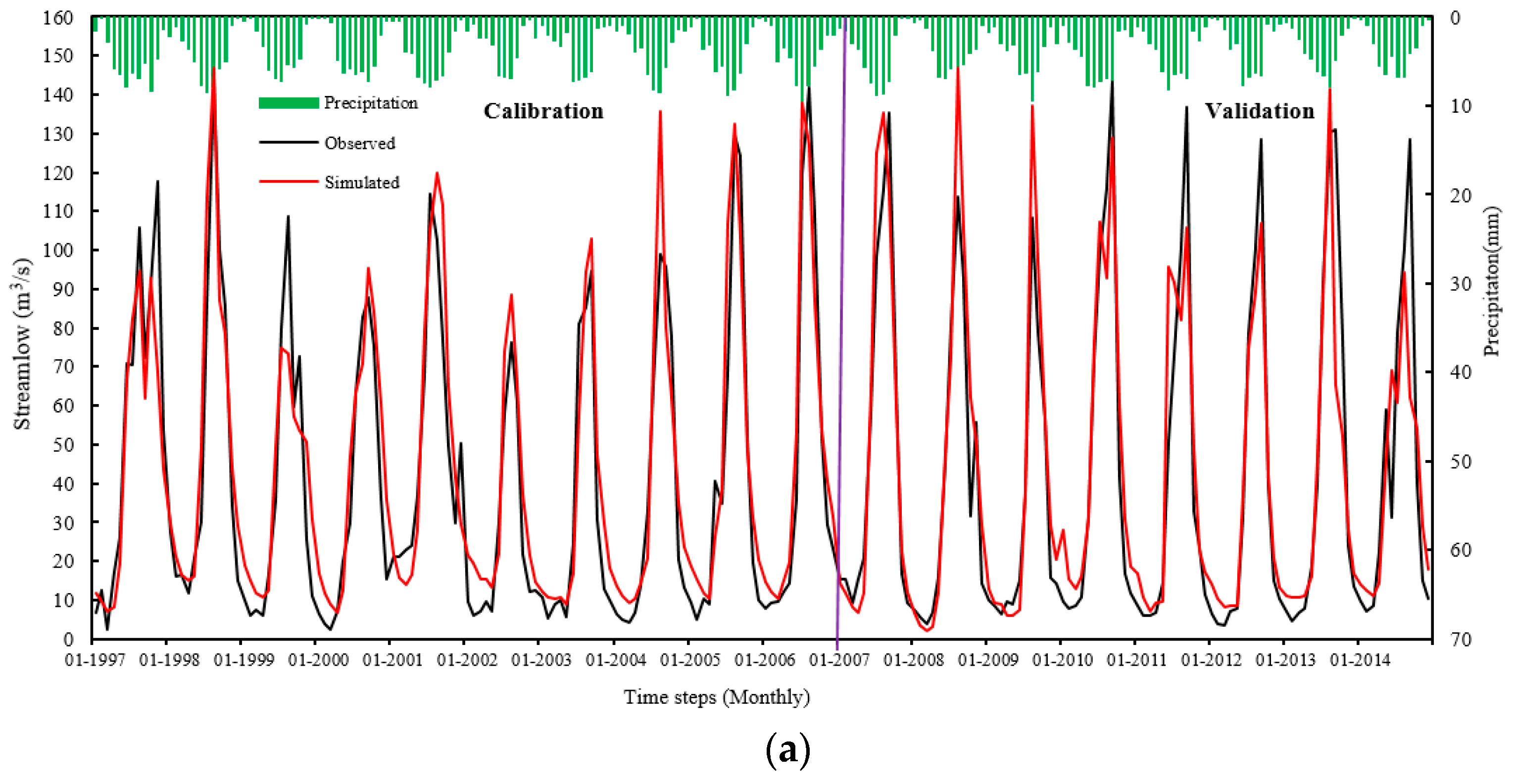
2.5. Model Calibration and Validation

SWAT is a sophisticated, robust, and interdisciplinary watershed modeling tool. However, the practical application of the hydrologic model to predict streamflow is determined by calibration and validation techniques [72,73,74,75]. It is helpful to find optimal parameters set with the optimum objective functions [74,76]. In the calibration process, parameters transferred from gauged to ungauged sites in data-scarce conditions could be affected by human activities [77]. Correct parameters make model calibration faster, more accurate, with low prediction uncertainty [66], and describe comprehensive hydrological processes [78]. However, model applications in different climatic regions are still challenged by a lack of historical data through the most commonly used watershed response variable in performance evaluation [44].

The SWAT Calibration and Uncertainty Program (SWAT-CUP) was developed to quantify SWAT model calibration, validation, and sensitivity analysis [63]. The capability of the SWAT-CUP encompasses an automated approach to conduct performance analysis more rigorously [66,72]. SWAT-CUP integrates various techniques in one interface that is easy to use and efficient [79]. The SWAT-CUP is an open-access program that connects the Sequential Uncertainty Fitting Version 2 (SUFI-2) algorithm to the SWAT model output [44]. The SUFI-2 accounts for all causes of uncertainty driving factors in water resources [72,79]. Sensitivity analysis determines model output changes regarding model input changes [65]. This study supported the auto analysis using SWAT-CUP and SUFI-2. An auto analysis attains suitable parameter estimates consistent with historical data to decide and refine estimates [80].

A sensitivity analysis affords reflections that limit output variances due to input variability [72]. The t-stat measures the sensitivity, and the p-values decide the implications [75]. A p-value close to zero has a meaningful value: the larger the t-stat value, the lesser the p-value, and the more sensitive the parameter [72]. The practical optimized value within a given bound minimizes the relative error [66]. Model validation indicates that a given model can produce accurate predictions without changing parameter values during calibration [81]. The observed and simulated annual streamflow was used to calibrate (1997–2006) and validate the (2007–2014) effects of LULC changes on GRSURQ. After calibration and validation, the impacts and implications of LULC change on GRSURQ have been analyzed.

2.6. Estimation of Model Predictive Accuracy

Statistical indicators were evaluated using SWAT-CUP to measure the best parameter [77]. The coefficient of determination (R²), Nash–Sutcliffe efficiency coefficient (NSE), and percent bias (PBIAS) were used to define the dependability of forecasts compared to experimental values of SWAT model performance. R² describes the percentage of variance to indicate the correlations between simulated and observed values. R² ranges from 0 to 1, where close to 1 and 0 show excellent and poor data presentation [80,82,83,84]. NSE assesses the predictive power and overall agreement of simulated and observed hydrographs. For acceptable model performance, NSE should be close to 1. PBIAS measures the normal tendency of simulated data with observed data [80]. The model performance ratings were evaluated based on a range of values for R², NSE, and PBIAS, as shown by Equations (2), (3), and (4), respectively.

$${\mathrm{R}}^2=\frac{{\left[{{\displaystyle \sum }}_{\mathrm{i}=1}^{\mathrm{n}}\left({\mathrm{Q}}_{\mathrm{si}}-{\overline{\mathrm{Q}}}_{\mathrm{si}}\right) \left({\mathrm{Q}}_{\mathrm{oi}}-{\overline{\mathrm{Q}}}_{\mathrm{o}}\right)\right]}^2}{{{\displaystyle \sum }}_{\mathrm{i}=1}^{\mathrm{n}}{({\mathrm{Q}}_{\mathrm{si}}-{\overline{\mathrm{Q}}}_{\mathrm{si}})}^2{{\displaystyle \sum }}_{\mathrm{i}=1}^{\mathrm{n}}{({\mathrm{Q}}_{\mathrm{oi}}-{\overline{\mathrm{Q}}}_{\mathrm{o}})}^2}$$

(2)

$$\mathrm{NSE}=1-\frac{{{\displaystyle \sum }}_{\mathrm{i}=1}^{\mathrm{n}}{({\mathrm{Q}}_{\mathrm{oi} }-{ \mathrm{Q}}_{\mathrm{si}})}^2}{{{\displaystyle \sum }}_{\mathrm{i}=1}^{\mathrm{n}}{({\mathrm{Q}}_{\mathrm{oi}}-{\overline{\mathrm{Q}}}_{\mathrm{oi}})}^2}$$

(3)

$$\mathrm{PBIAS}=\left[\frac{{{\displaystyle \sum }}_{\mathrm{i}=1}^{\mathrm{n}}{\mathrm{Q}}_{\mathrm{oi}}-{{\displaystyle \sum }}_{\mathrm{i}=1}^{\mathrm{n}}{\mathrm{Q}}_{\mathrm{si}}}{{{\displaystyle \sum }}_{\mathrm{i}=1}^{\mathrm{n}}{\mathrm{Q}}_{\mathrm{oi}}}\right]\times 100$$

(4)

where: Q_si (simulated value),

Q_oi (measured value), ${ \mathrm{Q} ¯}_{\mathrm{si}}$ and ${ \mathrm{Q} ¯}_{\mathrm{oi}}$ (mean of simulated and observed discharge, respectively).

3. Results and Discussion

3.1. SWAT Model Sensitivity Analysis

Hydrologic modeling and simulation were performed using the QSWAT in the QGIS environment. After preparing all model inputs, the model was simulated. Then, the sensitivity analysis was performed at the Asendabo station of the main Gilgel Gibe River. The sensitivity analysis identifies the most responsive hydrological parameters that significantly influence specific model output to enhance the reliability of results. The monthly streamflow data simulation was performed for 12 years, from 1997 to 2006. The sensitivity was determined using the t-stat and p-values provided by the SUFI-2 program. In these statistics, the higher the t-stat values, the greater the relative sensitivity. The p-values were used to fix the sensitivity implication so that the closer the p-values to zero, the more critical the parameters become. Before calibration and validation, many more parameters were used to identify the most sensitive parameters that govern streamflow generation. Then, the 14 most sensitive parameters were selected to calibrate and validate model predictive capability based on sensitivity evaluation criteria. The parameter values were adjusted by changing parameters at a time within acceptable ranges until the best simulation was attained [70]. The selected most sensitive parameters and their relatively optimized values are indicated in

Table 1. Sensitive model calibration parameters and optimized values for LULC-2000 simulation.

Parameter Name	Description	Range	Optimized Value
R_CN2.mgt	Curve number for moisture condition II	−0.02–0.2	0.077
V_ALPHA_BF.gw	Coefficient of depletion of groundwater	0.01–1	0.120
V_ESCO.hru	Soil evaporation compensation factor	0–1	0.069
V_GW_DELAY.gw	Groundwater delay	0–350	195.650
V_GW_REVAP.gw	Groundwater “revap” coefficient	0.02–0.2	0.091
V_CANMX.hru	Maximum canopy storage	10–100	70.570
V_EPCO.hru	Plant uptake compensation factor	0–1	0.649
V_CH_K2.rte	Effective hydraulic conductivity	0.01–150	118.052
R_SOL_AWC().sol	Available water capacity of the soil	−0.5–0.5	0.403
R_SOL_K().sol	Saturated hydraulic conductivity	−0.5–0.5	−0.443
V_SURLAG.bsn	Surface runoff lag coefficient	0–24	12.744
V_SHALLST.gw	Initial depth of the shallow aquifer	0–500	404.450
R_SOL_Z().sol	Soil depth	0.5–1	0.681
R_GWQMN.gw	Threshold depth of shallow water aquifer	0–2	0.242

with qualifiers. The parameter qualifier (R_) refers to the default value multiplied by (1 plus an optimized value), and (V_) refers to the replacement of the default value with an optimized one. The extensions .hru, .mgt, .bsn, .gw, .sol, and .rte indicate the SWAT parameter family of HRU, management, basin, groundwater, soil, and route, respectively.

The model was calibrated and validated to evaluate model simulation performance in the watershed under changing environments due to extensive human-induced factors. LULC change uncertainty substantially influences hydrologic cycles, complicating groundwater recharge and surface runoff modeling outputs [8]. Model parameters are usually calibrated under one LULC scenario, and are then supposed to be time-invariant while simulating different hydrological LULC scenarios. However, other variables of LULC affect simulations to quantify streamflow variability for a new LULC scenario. Through anthropogenic activities, ensuing changes in the watershed feature that model parameters are not appropriate for other LULC situations [5,8,17]. As calibration parameters differ while LULC changes, using the same parameters may not always be feasible. The simulations change when LULC adjustments affect HRU configurations; this no longer affects the new LULC simulation. The attributes of HRUs are the significant influences affecting streamflow and other hydrologic components.

Consequently, in the present study, simulations of each reference LULC period were calibrated using an auto-calibration technique to optimize the values of sensitive parameters. In addition, new parameters were included to check whether the previously applied parameter could represent the hydrologic simulation process or not. Nevertheless, optimal values and parameter substitutions were observed regardless of the similarity of parameters for the 2010 and 2020 LULC simulation periods. Hence, the calibration for simulation of 2010 and 2020 LULC indicates that CN2, GW_DELAY, GW_REVAP, ALPHA_BF, ESCO, EPCO, CH_K2, RCHRG_DP, SOL_AWC, SOL_K, and GWQMN were newly optimized best parameters with replacement and multiplication of actual simulation results. This might support reliable land and water resource development plans.

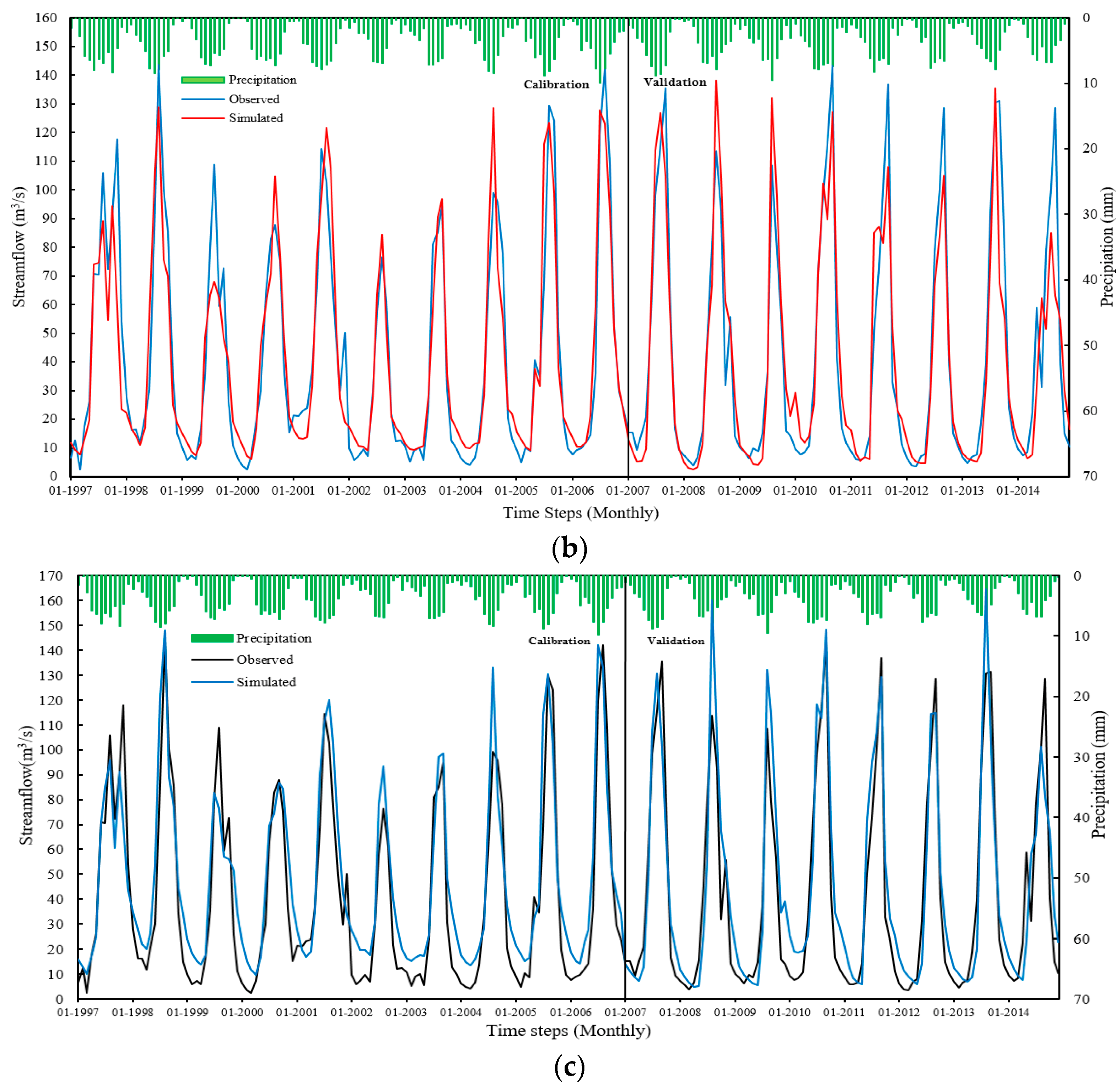
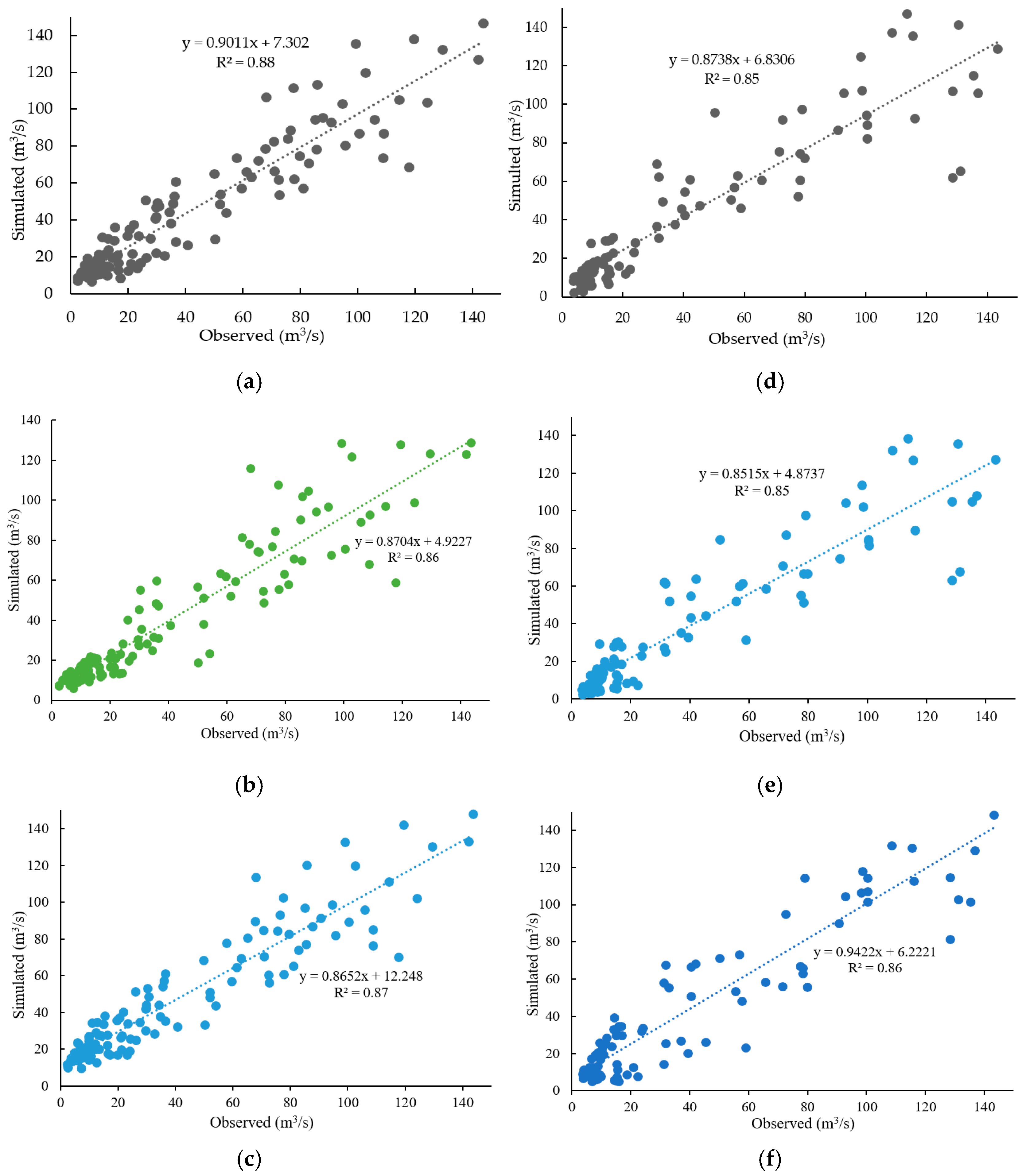
3.2. Assessing Hydrological Model Performance on Streamflow

SWAT-CUP application with SUFI-2 set of rules has been employed for calibration, validation, and uncertainty assessment of SWAT output. This study calibrated the model to make the simulation result more realistic for the independent calibration time steps. The statistically significant model performance among time intervals was judged based on recommendations given in Moriasi et al. [75,76], the coefficient of determination (R²), Nash and Sutcliffe’s model efficiency (NSE), and percentage bias (PBIAS). The hydrology is well-simulated and is considered representative of the watershed if the statistical indicators R², NSE, PBIAS, and graphical fitness are satisfied. The calibration period of the SWAT model was (1997–2006), excluding two years of model warmup periods and its validation period (2007–2014). R², NSE, and PBIAS compared the model’s applicability. R² suggests that the observed and simulated values are in good agreement as it is close to one. PBIAS characterizes the error among the experimental and simulated values as a percentage. The objective functions were within the acceptable range of goodness of fit tests [75]. The model performance showed that statistical values simulating monthly streamflow were R², NSE, and PBIAS of 0.88, 0.87, and −7.9%, respectively, during the calibration time steps of the 2000 land use simulation. Model validation results should increase user confidence in model predictive capabilities [76]. The model was validated with observed flow data for eight years (2007–2014) without further adjusting calibration parameters. The SWAT overall performance for the 2000 LULC simulation during validation was 0.85, 0.85, and −4.0% for R², NSE, and PBIAS, respectively.

As depicted in Figure 4a–c, the hydrographs indicated that the results were in good agreement with measured and simulated streamflow data. The selected statistical performance indicators show that there is good agreement for both calibration and validation periods (R² & NSE > 0.84, −15 < PBIAS < +15), which are in reasonably acceptable ranges as in [75,76]. The positive and negative results of PBIAS showed underestimation and overestimation, respectively. Hence, during the model’s second simulation, the model overestimated (1%, 3%) calibration and validation time steps, respectively. Moreover, the PBIAS (−7.9% and −4.0%) for calibration and validation, respectively, indicates that the model was underestimated by (7.9%, 4.0%) for 2000 and (14.3%, 9.3%) for 2020 land use periods (

Table 2. Statistical performance indicators during calibration and validation LULC periods.

Variable	2000		2010		2020
	Calibration	Validation	Calibration	Validation	Calibration	Validation
R2	0.88	0.85	0.86	0.85	0.87	0.86
NSE	0.87	0.85	0.86	0.85	0.84	0.85
PBIAS	−7.9	−4.0	1.0	3.0	−14.3	−9.3

) during calibration and validation time steps. As revealed in Figure 5a–c for calibration and Figure 5d–f for validation, the scattered plot of the observed and simulated streamflow, the best-fit line’s correlation coefficient of (0.88, 0.86, 0.87) during calibration and (0.85, 0.85, 0.86) during validation time steps is observed for 2000, 2010, and 2020 land use periods, respectively. The statistical performance evaluation results have been statistically accurate for all calibration and validation time steps.

Statistical values (Table 2) indicate that objective functions were acceptable for model evaluation [75,76]. Several authors [14,23,36,40,57,62] calibrated the SWAT model in other Ethiopian watersheds. They mainly reported statistical performance indicators of R², NSE, and PBIAS based on [75], comparable with the present findings. The resulting statistics were comparable to other worldwide studies [35,48,49,50,51,52,53,77]. The SURQ relies upon overall precipitation, evaporation, and soil water storage. The most considerable SURQ is derived from high precipitation and elevation. The most increased flows are typical from July to September, and the lowest flows occur during February and May. A regular correlation between rainfall and runoff was observed (Figure 4a–c). Accordingly, the applicability of the simulated SWAT model was found to be in agreement with regional and global studies and was reasonably acceptable in the Gilgel Gibe watershed.

SWAT was found to be reasonably appropriate for estimating the spatiotemporal variability of GRSURQ in the Gilgel Gibe watershed. Therefore, the simulated hydrological parameters can be helpful in the planning and management of water resource projects. The SWAT model was simulated, properly calibrated, validated, and confirmed to assess the impact of LULC on the watershed’s hydrology. The performance of simulated and measured results suggests that SWAT properly represents the streamflow modeling. Furthermore, the results indicated that the SWAT model performs well. Hence, the calibrated model can be used to analyze the effect of climate and LULC change on groundwater abstraction and drought extremes. Thus, this can be improved with integrated surface water and groundwater interaction of abstraction scenarios to assess the impact on rivers drying up or groundwater depletion. Consequently, the model output can support the water resource decision-making process.

3.3. Effects and Implications of LULC Change

In watershed hydrology, understanding LULC change will empower planners and policy-makers to reduce adverse effects. The forest covers have undergone deforestation and decreased by 5.4936%. The barren land has been entirely transformed by 0.001% of other activities. The urban/built-up land classes have increased by 0.4511% over the last two decades. Agricultural land covered about 77.6760%, 80.8945%, and 81.4319% of the entire watershed in 2000, 2010, and 2020. Assessment of LULC over a long time confirmed continuous agricultural activity and deforestation. The agricultural land use was augmented by 3.2184% from 2000 to 2010 and 0.5374% from 2010 to 2020. During the last two decades, agricultural land has increased significantly by 3.7558% from 2000 to 2020. The artificial surfaces have proven to be 0.0416% from 2000 to 2010, 0.4094% from 2010 to 2020, and 0.4510% from 2000 to 2020. An increase in agricultural land results in a reduction of forested areas and grassland. Accordingly, the forested land area changed by −5.6942%, +0.2006%, and −5.4936% from 2000–2010, 2010–2020, and 2000–2020. The grassland change was observed to be +2.5079%, −1.1485%, and +1.3594% from 2000–2010, 2010–2020, and 2000–2020, respectively. The available bare lands in 2000 have completely transformed into other LULC types. The implications acquired for 2000 show that forested area land covers were 9.8708% but decreased by 5.6942% in 2010 and 5.4936% in 2020.

Similarly, grassland cover was 13.360% in 2000, increased by 2.5079% in 2010, but decreased by 1.1485% in 2020. Numerous anthropogenic activities associated with socio-economic and biophysical environments reduced forested areas. The effects showed significant variations in LULC that occurred from 2000 to 2010. From a political atmosphere point of view, it could be regarded that poor development policy, globalization, and market forces of multi-national initiatives drive LULC changes. It has been hypothesized that LULC change results from favorable economic and institutional conditions triggered by the expansion of agriculture and rangelands.

LULC disturbs water budgets by reducing infiltration and increasing surface runoff in the watershed. Human activities in the biophysical environment increase reliance on agriculture. The expansion of cultivation is to produce a crop at the expense of forests and grazing lands. This increases land susceptibility to erosion and sedimentation of water bodies and reservoirs. This is attributed to the loss of fertile topsoil, soil degradation, the decline in organic matter, decreased plant-available water, and nutrient loss, reducing crop yields. Agricultural land increases as the population increases, which is the reason for the cultivation of farming products. LULC changes in the watershed have been altered extensively because of human activities. There is a change in vegetation and forestlands due to agriculture-affected water bodies in the ecosystem and land surfaces. The agricultural land use practice encourages more surface runoff than infiltration. Hence, LULC change impact on spatiotemporal assessment is substantial for socio-economic and environmental development. The findings are in agreement with studies conducted by [6,17,20,21,22,23,29,56]. Similar studies confirmed that LULC changed from forest to agricultural land, waterbody, industrial farmland, and built-up areas.

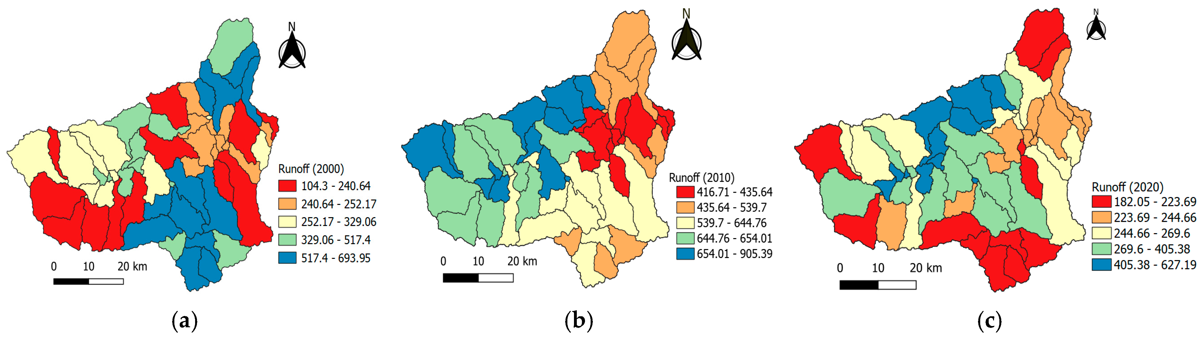
3.4. Effects and Implications of LULC Change on Surface Runoff

LULC change usually induces significant changes in flood peak and infiltration properties, thus affecting the entire hydrological condition of the watershed. Assessing the spatiotemporal variability, the effect, and the implications of LULC changes is essential to estimating water balances. Computational reliability of hydrological model simulation increases with well-calibrated model simulation. In the present study, the SWAT model was initially calibrated using the LULC map of 2000, then updated to 2010 and 2020 to examine the effect of LULC changes on GRSURQ. For the first LULC-2000 period, the watershed has a total mean annual value of actual evapotranspiration of 608.61 mm, groundwater contribution to streamflow of 313.28 mm, lateral flow of 75.9 mm, recharge of 348.16 mm, SURQ 347.9 mm, and water yield 754.52 mm. The simulated annual water balances indicated that actual evapotranspiration loses 44% of the yearly precipitation and 56% of the rainfall in the watershed contributes to the streamflow during the simulation period. The average annual contribution of groundwater relative to rainfall is 22.7%. Therefore, 25.22% of precipitation is lost as groundwater recharge.

Surface runoff is the primary integral part of streamflow and is essential in estimating groundwater recharge potential. LULC is a significant characteristic of the surface runoff process that affects soil water content, water yield, infiltration rate, and groundwater flow. In watershed hydrology, surface runoff is the prime streamflow contribution to aquifers. The simulated total average surface runoff in 2000, 2010, and 2020 was 347.9 mm, 599.36 mm, and 282.99 mm, respectively. The results of the LULC changes indicated that surface runoff increased in 2010 and decreased in 2020. In the second decade, a decrease in surface runoff and water yield increased groundwater recharge. In high slope areas, there is no infiltration, and precipitation cannot recharge, resulting in an increased volume of surface runoff. The other reason for reducing surface runoff is the excellent watershed management practice promoted by the government and local administration in the last decade. If not adequately managed, the time to peak flow is reduced, causing flooding and affecting lives and property. The model simulated high water yield from June to September as precipitation increased from June to August in the summer.

Consequently, excess water flows can be stored and used during low flow conditions. The simulated streamflow accounts for the LULC change scenarios classified into moist (August to October) and dry months (February to April). As a result, surface runoff was very high during the wet season and low during the dry. This evaluation showed that the increment of cultivated land causes a direct runoff throughout the wettest months. The increase in surface runoff simulated during the wet season due to LULC changes has broader ecological resource development implications. The increase in runoff may have broader implications for growing soil erosion and sedimentation, if proper control is not implemented. It also removes the top productive soil and causes degradation, affecting agricultural land, natural river banks, and low plain areas. This reduces crop yield and leads to food insecurity and sediment inflow to downstream reservoirs, decreasing the life span of service reservoirs and hydraulic structures. The SURQ map suggests that sub-basins with high rainfall correspond to extreme runoff (Figure 6a–c). For all LULC reference periods, the sub-basin numbers (8, 19, 22, and 39) in 2000, (50–53) in 2010, and 2020 were highly attributed to the surface runoff of 104.29 mm to 905.39 mm annually. High annual surface runoff is observed in the highland elevation areas, attributed to the high rainfall and steep slope topography. In flat-sloping regions of low lands, surface runoff is also higher on cultivated land, resulting in human activities in the watershed and significant driving factors for LULC change. These findings agree with other similar efforts [5,14,34,35,36,38,85].

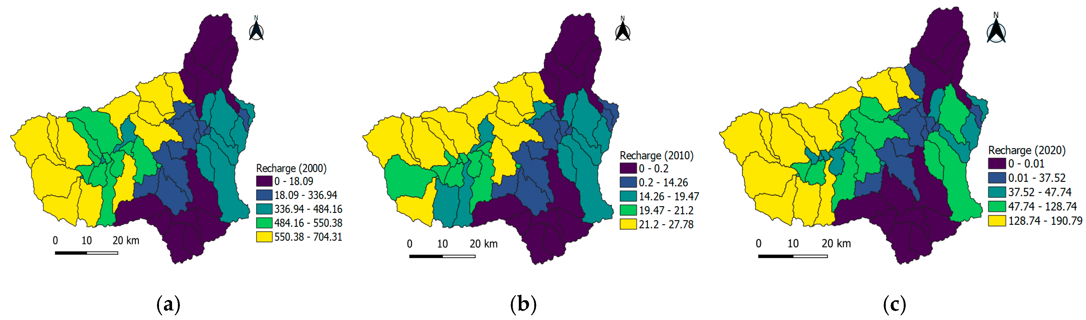
3.5. Effects and Implications of LULC Change on Groundwater Recharge

Groundwater recharge is a vital hydrologic cycle for sustaining aquifers recharged through precipitation and recharged artificially through human activity. Hence, developing the best management scenarios would help conserve stream biotas within the ecosystems by increasing recharge and decreasing surface runoff [18]. Best management scenarios increase groundwater recharge and decrease surface runoff, reducing erosion as in-stream sediment loads decrease. For example, converting agricultural land back to natural land cover decreased surface runoff. In addition, it decreased in-stream sediment loads due to reduced erosion. It has been observed that from 2010 to 2020, soils recovering to natural land conditions had a lower bulk density, higher saturated hydraulic conductivity, and decreased surface runoff. In addition, surface runoff was affected by LULC change and increased when the interception decreased as forest cover decreased. Poor land-use practices alter soil structure and porosity, reduce infiltration rate, and increase surface runoff. However, intensive agricultural practices removing vegetation covers exposed dense soils to erosion, decreasing groundwater recharge in the aquifer.

LULC strongly influences groundwater recharge, and it is essential to understand its interactions with increasing natural and human activities. The calibrated SWAT model estimated that the simulated groundwater recharge for the LULC reference periods 2000, 2010, and 2020 averages 348.16 mm, 13.59 mm, and 76.37 mm, respectively. At the sub-basin scale, groundwater recharge varies from 0 to 704.31, 0 to 27.8, and 0 to 190.79 mm for 2000, 2010, and 2020, respectively. The sub-basin numbers (35, 50–53), (50–53), and (35, 27, 44, 51) for 2000, 2010, and 2020 were attributed to high groundwater recharge. Rangeland and sandy, loamy soil allow alluvial deposits to infiltrate the sub-surface. The spatial pattern of GRSURQ showed the direct effects of surface runoff reducing the recharge rate (Figure 6a–c and Figure 7a–c). The lowest recharge values are observed in forest-dominated sub-basins. The decline in streamflow is attributed to lower surface runoff due to increasing forestland, which advances the water holding capacity of the soil, reducing infiltration and recharge conditions. The low recharge estimates in the flat areas could be due to heavy clay soils with low infiltration. The decrease in groundwater recharge could be attributed to high evapotranspiration. It increases recharge and runoff for water resource control strategies tailored to the watershed.

The variabilities of mean yearly groundwater recharge found in the three reference periods of this study were lower than other watershed recharge rates [13]. Moreover, the 2010 LULC simulation groundwater recharge was much lower than the estimated rate [86]. The temporal variation of groundwater recharge showed that the highest value occurred during the wet months (June to August). The LULC simulation scenarios dry season flow (December to April) had shown lowering responses of groundwater recharge during dry periods. Therefore, the study deduced that the SWAT model underestimated and overestimated the high flow rate during low flow. The main reason for reducing the average annual groundwater recharge is the long dry season from December to May, before the wet season. These changes improved the wet seasonal flow and decreased dry seasonal flow. The findings revealed increasing wet flow (June–September) and lower dry flow due to alteration of vegetation cover in agricultural lands over study periods.

Similar efforts in Ethiopia reported that expansion of agricultural land diminishing forest, shrubland, and grasslands increased runoff, decreasing recharge [14,23,26,36,54]. This produces flooding during the rainy season, decreasing low flow during the dry period. Therefore, reduced recharge due to LULC change revealed a probable recurrent hydrological drought. Understanding its effect on GRSURQ is essential to knowing the flow regimes of wet and dry seasons in the watershed. Hence, there should be an effort to enhance watershed management practices for efficient use of resources for national socio-economic development. Hence, sustainable land and water management is crucial to safeguard the environmental and riverine ecosystems.

4. Conclusions

The present study examined spatiotemporal effects and implications of LULC changes on groundwater recharge and surface runoff (GRSURQ) under three reference scenarios in the Gilgel Gibe, an East African watershed. The SWAT model was built and simulated using DEM, LULC, soil, weather, and hydrological data to understand GRSURQ over the watershed. LULC changes derived from satellite images showed an increase in agricultural lands (3.76%) and a decline in forestland (5.49%) and grassland (2.51%) due to population growth and associated human activities. The effects reveal that the forests have undergone deforestation and were reduced due to a change in the considerable agricultural activity in the watershed.

The ability of the SWAT model to satisfactorily simulate stream flows was evaluated using SWAT-CUP, SUFI-2. The coefficient of determination (R²), Nash–Sutcliffe efficiency (NSE), and percent bias (PBIAS) for calibration and validation showed excellent agreement between observed and simulated hydrographs. The results found that R2, NSE, and PBIAS values were in acceptable ranges for all LULC simulations. The results suggest that LULC changes substantially affect the watershed GRSURQ. The calibrated model confirmed an increase in runoff and a decline in recharge because of changes in LULC. The study scrutinized the impact of LULC changes on GRSURQ, which is mainly due to intensive agricultural expansion and withdrawal of the forestlands. In addition, the increase in agricultural land practice is related to water abstraction for household consumption, resulting in reduction in ground recharge. The increase in surface runoff and the decline of groundwater recharge during the wet season could lead to water scarcity during the dry season, bringing about an aquifer drought. Therefore, developing watershed management scenarios is indispensable in reducing the adverse effect of LULC changes on GRSURQ.

Therefore, an enormous concern with LULC response is imperative for planners and policy-makers of water resource projects to ensure ecosystem sustainability. Furthermore, if adequately assessed, the effects of human-induced LULC changes are indispensable in understanding hydrologic dynamics. Hence, it was found that providing insights into calibrated results helps to contribute to a concrete plan for future management strategies on watershed hydrology. Therefore, the calibrated model setup can be an ensemble for further assessment, integrating with groundwater flow modeling under different scenarios and driving factors that might influence groundwater storage.

References

1. Lal, R. World Water Resources and Achieving Water Security. Agron. J. 2015, 107, 1526–1532. [Google Scholar] [CrossRef] [Green Version]
2. Scanlon, B.R.; Jolly, I.; Sophocleous, M.; Zhang, L. Global impacts of conversions from natural to agricultural ecosystems on water resources: Quantity versus quality. Water Resour. Res. 2007, 43, W03437. [Google Scholar] [CrossRef] [Green Version]
3. Foley, J.A.; DeFries, R.; Asner, G.P.; Barford, C.; Bonan, G.; Carpenter, S.R.; Chapin, F.S.; Coe, M.T.; Daily, G.C.; Gibbs, H.K.; et al. Global Consequences of Land Use. Science 2005, 309, 570–574. [Google Scholar] [CrossRef] [PubMed] [Green Version]
4. Scanlon, B.R.; Reedy, R.C.; Stonestrom, D.A.; Prudic, D.E.; Dennehy, K.F. Impact of land use and land cover change on groundwater recharge and quality in the southwestern US. Glob. Chang. Biol. 2005, 11, 1577–1593. [Google Scholar] [CrossRef]
5. Guzha, A.C.; Rufino, M.C.; Okoth, S.; Jacobs, S.; Nóbrega, R.L.B. Impacts of land use and land cover change on surface runoff, discharge and low flows: Evidence from East Africa. J. Hydrol. Reg. Stud. 2018, 15, 49–67. [Google Scholar] [CrossRef]
6. Bewket, W.; Sterk, G. Dynamics in land cover and its effect on stream flow in the Chemoga watershed, Blue Nile basin, Ethiopia. Hydrol. Process. 2005, 19, 445–458. [Google Scholar] [CrossRef]
7. Owuor, S.O.; Butterbach-Bahl, K.; Guzha, A.C.; Rufino, M.C.; Pelster, D.E.; Díaz-Pinés, E.; Breuer, L. Groundwater recharge rates and surface runoff response to land use and land cover changes in semi-arid environments. Ecol. Process. 2016, 5, 16. [Google Scholar] [CrossRef] [Green Version]
8. Mensah, J.K.; Ofosu, E.A.; Yidana, S.M.; Akpoti, K.; Kabo-bah, A.T. Integrated modeling of hydrological processes and groundwater recharge based on land use land cover, and climate changes: A systematic review. Environ. Adv. 2022, 8, 100224. [Google Scholar] [CrossRef]
9. Taylor, R.G.; Scanlon, B.; Döll, P.; Rodell, M.; van Beek, R.; Wada, Y.; Longuevergne, L.; Leblanc, M.; Famiglietti, J.S.; Edmunds, M.; et al. Ground water and climate change. Nat. Clim. Chang. 2013, 3, 322–329. [Google Scholar] [CrossRef] [Green Version]
10. Coelho, V.H.R.; Montenegro, S.; Almeida, C.N.; Silva, B.; Oliveira, L.M.; Gusmão, A.C.V.; Freitas, E.S.; Montenegro, A.A.A. Alluvial groundwater recharge estimation in semi-arid environment using remotely sensed data. J. Hydrol. 2017, 548, 1–15. [Google Scholar] [CrossRef]
11. Pavelic, P. Groundwater Availability and Use in Sub-Saharan Africa: A Review of 15 Countries; International Water Management Institute (IWMI): Colombo, Sri Lanka, 2012; ISBN 9789290907589. [Google Scholar]
12. Scanlon, B.R.; Keese, K.E.; Flint, A.L.; Flint, L.E.; Gaye, C.B.; Edmunds, W.M.; Simmers, I. Global synthesis of groundwater recharge in semiarid and arid regions. Hydrol. Process. 2006, 20, 3335–3370. [Google Scholar] [CrossRef]
13. Mengistu, T.D.; Chung, I.-M.; Chang, S.W.; Yifru, B.A.; Kim, M.-G.; Lee, J.; Ware, H.H.; Kim, I.-H. Challenges and Prospects of Advancing Groundwater Research in Ethiopian Aquifers: A Review. Sustainability 2021, 13, 11500. [Google Scholar] [CrossRef]
14. Gessesse, A.A.; Melesse, A.M.; Abera, F.F.; Abiy, A.Z. Modeling Hydrological Responses to Land Use Dynamics, Choke, Ethiopia. Water Conserv. Sci. Eng. 2019, 4, 201–212. [Google Scholar] [CrossRef]
15. Carter, R.C.; Parker, A. Climate change, population trends and groundwater in Africa. Hydrol. Sci. J. 2009, 54, 676–689. [Google Scholar] [CrossRef] [Green Version]
16. Wada, Y.; van Beek, L.P.H.; van Kempen, C.M.; Reckman, J.W.T.M.; Vasak, S.; Bierkens, M.F.P. Global depletion of groundwater resources. Geophys. Res. Lett. 2010, 37, L20402. [Google Scholar] [CrossRef] [Green Version]
17. Woldesenbet, T.A.; Elagib, N.A.; Ribbe, L.; Heinrich, J. Hydrological responses to land use/cover changes in the source region of the Upper Blue Nile Basin, Ethiopia. Sci. Total Environ. 2017, 575, 724–741. [Google Scholar] [CrossRef]
18. Guida-Johnson, B.; Zuleta, G.A. Land-use land-cover change and ecosystem loss in the Espinal ecoregion, Argentina. Agric. Ecosyst. Environ. 2013, 181, 31–40. [Google Scholar] [CrossRef]
19. Haregeweyn, N.; Tsunekawa, A.; Poesen, J.; Tsubo, M.; Meshesha, D.T.; Fenta, A.A.; Nyssen, J.; Adgo, E. Comprehensive assessment of soil erosion risk for better land use planning in river basins: Case study of the Upper Blue Nile River. Sci. Total Environ. 2017, 574, 95–108. [Google Scholar] [CrossRef] [PubMed] [Green Version]
20. Zeleke, G.; Hurni, H. Implications of land use and land cover dynamics for mountain resource degradation in the Northwestern Ethiopian highlands. Mt. Res. Dev. 2001, 21, 184–191. [Google Scholar] [CrossRef] [Green Version]
21. Moges, D.M.; Bhat, H.G. An insight into land use and land cover changes and their impacts in Rib watershed, north-western highland Ethiopia. Land Degrad. Dev. 2018, 29, 3317–3330. [Google Scholar] [CrossRef]
22. Demissie, F.; Yeshitila, K.; Kindu, M.; Schneider, T. Land use/Land cover changes and their causes in Libokemkem District of South Gonder, Ethiopia. Remote Sens. Appl. Soc. Environ. 2017, 8, 224–230. [Google Scholar] [CrossRef]
23. Getu Engida, T.; Nigussie, T.A.; Aneseyee, A.B.; Barnabas, J. Land Use/Land Cover Change Impact on Hydrological Process in the Upper Baro Basin, Ethiopia. Appl. Environ. Soil Sci. 2021, 2021, 6617541. [Google Scholar] [CrossRef]
24. Regasa, M.S.; Nones, M.; Adeba, D. A Review on Land Use and Land Cover Change in Ethiopian Basins. Land 2021, 10, 585. [Google Scholar] [CrossRef]
25. Hailu, A.; Mammo, S.; Kidane, M. Dynamics of land use, land cover change trend and its drivers in Jimma Geneti District, Western Ethiopia. Land Use Policy 2020, 99, 105011. [Google Scholar] [CrossRef]
26. Birhanu, A.; Masih, I.; van der Zaag, P.; Nyssen, J.; Cai, X. Impacts of land use and land cover changes on hydrology of the Gumara catchment, Ethiopia. Phys. Chem. Earth 2019, 112, 165–174. [Google Scholar] [CrossRef]
27. Dibaba, W.T.; Demissie, T.A.; Miegel, K. Drivers and Implications of Land Use/Land Cover Dynamics in Finchaa Catchment, Northwestern Ethiopia. Land 2020, 9, 113. [Google Scholar] [CrossRef] [Green Version]
28. Zewdie, M.; Worku, H.; Bantider, A. Temporal Dynamics of the Driving Factors of Urban Landscape Change of Addis Ababa During the Past Three Decades. Environ. Manag. 2018, 61, 132–146. [Google Scholar] [CrossRef]
29. Tsegaye, D.; Moe, S.R.; Vedeld, P.; Aynekulu, E. Land-use/cover dynamics in Northern Afar rangelands, Ethiopia. Agric. Ecosyst. Environ. 2010, 139, 174–180. [Google Scholar] [CrossRef]
30. Biazin, B.; Sterk, G. Drought vulnerability drives land-use and land cover changes in the Rift Valley dry lands of Ethiopia. Agric. Ecosyst. Environ. 2013, 164, 100–113. [Google Scholar] [CrossRef]
31. Dile, Y.T.; Tekleab, S.; Ayana, E.K.; Gebrehiwot, S.G.; Worqlul, A.W.; Bayabil, H.K.; Yimam, Y.T.; Tilahun, S.A.; Daggupati, P.; Karlberg, L.; et al. Advances in water resources research in the Upper Blue Nile basin and the way forward: A review. J. Hydrol. 2018, 560, 407–423. [Google Scholar] [CrossRef]
32. Githui, F.; Mutua, F.; Bauwens, W. Estimating the impacts of land-cover change on runoff using the soil and water assessment tool (SWAT): Case study of Nzoia catchment, Kenya/Estimation des impacts du changement d’occupation du sol sur l’écoulement à l’aide de SWAT: Étude du cas du bassi. Hydrol. Sci. J. 2009, 54, 899–908. [Google Scholar] [CrossRef]
33. Hailemariam, S.; Soromessa, T.; Teketay, D. Land Use and Land Cover Change in the Bale Mountain Eco-Region of Ethiopia during 1985 to 2015. Land 2016, 5, 41. [Google Scholar] [CrossRef] [Green Version]
34. Mango, L.M.; Melesse, A.M.; McClain, M.E.; Gann, D.; Setegn, S.G. Land use and climate change impacts on the hydrology of the upper Mara River Basin, Kenya: Results of a modeling study to support better resource management. Hydrol. Earth Syst. Sci. 2011, 15, 2245–2258. [Google Scholar] [CrossRef] [Green Version]
35. Gyamfi, C.; Ndambuki, J.M.; Anornu, G.K.; Kifanyi, G.E. Groundwater recharge modelling in a large scale basin: An example using the SWAT hydrologic model. Model. Earth Syst. Environ. 2017, 3, 1361–1369. [Google Scholar] [CrossRef]
36. Gashaw, T.; Tulu, T.; Argaw, M.; Worqlul, A.W. Modeling the hydrological impacts of land use/land cover changes in the Andassa watershed, Blue Nile Basin, Ethiopia. Sci. Total Environ. 2018, 619–620, 1394–1408. [Google Scholar] [CrossRef]
37. Sterling, S.; Ducharne, A. Comprehensive data set of global land cover change for land surface model applications. Glob. Biogeochem. Cycles 2008, 22, GB3017. [Google Scholar] [CrossRef]
38. Jin, X.; Jin, Y.; Yuan, D.; Mao, X. Effects of land-use data resolution on hydrologic modelling, a case study in the upper reach of the Heihe River, Northwest China. Ecol. Modell. 2019, 404, 61–68. [Google Scholar] [CrossRef]
39. Santhi, C.; Allen, P.M.; Muttiah, R.S.; Arnold, J.G.; Tuppad, P. Regional estimation of base flow for the conterminous United States by hydrologic landscape regions. J. Hydrol. 2008, 351, 139–153. [Google Scholar] [CrossRef]
40. Setegn, S.G.; Srinivasan, R.; Dargahi, B. Hydrological Modelling in the Lake Tana Basin, Ethiopia Using SWAT Model. Open Hydrol. J. 2008, 2, 49–62. [Google Scholar] [CrossRef] [Green Version]
41. Suryavanshi, S.; Pandey, A.; Chaube, U.C. Hydrological simulation of the Betwa River basin (India) using the SWAT model. Hydrol. Sci. J. 2017, 62, 960–978. [Google Scholar] [CrossRef]
42. Arnold, J.G.; Srinivasan, R.; Muttiah, R.S.; Williams, J.R. Large Area Hydrologic Modeling and Assessment Part I: Model Development. J. Am. Water Resour. Assoc. 1998, 34, 73–89. [Google Scholar] [CrossRef]
43. Gassman, P.W.; Reyes, M.R.; Green, C.H.; Arnold, J.G. The Soil and Water Assessment Tool: Historical Development, Applications, and Future Research Directions. Trans. ASABE 2007, 50, 1211–1250. [Google Scholar] [CrossRef] [Green Version]
44. Abbaspour, K.C.; Yang, J.; Maximov, I.; Siber, R.; Bogner, K.; Mieleitner, J.; Zobrist, J.; Srinivasan, R. Modelling hydrology and water quality in the pre-alpine/alpine Thur watershed using SWAT. J. Hydrol. 2007, 333, 413–430. [Google Scholar] [CrossRef]
45. Srinivasan, R.; Ramanarayanan, T.S.; Arnold, J.G.; Bednarz, S.T. Large Area Hydrologic Modeling and Assessment Part II: Model Application. J. Am. Water Resour. Assoc. 1998, 34, 91–101. [Google Scholar] [CrossRef]
46. Arnold, J.; Muttiah, R.; Srinivasan, R.; Allen, P. Regional estimation of base flow and groundwater recharge in the Upper Mississippi river basin. J. Hydrol. 2000, 227, 21–40. [Google Scholar] [CrossRef]
47. Akoko, G.; Le, T.H.; Gomi, T.; Kato, T. A Review of SWAT Model Application in Africa. Water 2021, 13, 1313. [Google Scholar] [CrossRef]
48. Gyamfi, C.; Ndambuki, J.; Salim, R. Hydrological Responses to Land Use/Cover Changes in the Olifants Basin, South Africa. Water 2016, 8, 588. [Google Scholar] [CrossRef]
49. Chen, Y.; Niu, J.; Sun, Y.; Liu, Q.; Li, S.; Li, P.; Sun, L.; Li, Q. Study on streamflow response to land use change over the upper reaches of Zhanghe Reservoir in the Yangtze River basin. Geosci. Lett. 2020, 7, 6. [Google Scholar] [CrossRef]
50. Chen, Y.; Nakatsugawa, M. Analysis of Changes in Land Use/Land Cover and Hydrological Processes Caused by Earthquakes in the Atsuma River Basin in Japan. Sustainability 2021, 13, 13041. [Google Scholar] [CrossRef]
51. Astuti, I.S.; Sahoo, K.; Milewski, A.; Mishra, D.R. Impact of Land Use Land Cover (LULC) Change on Surface Runoff in an Increasingly Urbanized Tropical Watershed. Water Resour. Manag. 2019, 33, 4087–4103. [Google Scholar] [CrossRef]
52. Huang, T.C.C.; Lo, K.F.A. Effects of land use change on sediment and water yields in yang ming shan national park, taiwan. Environments 2015, 2, 32–42. [Google Scholar] [CrossRef] [Green Version]
53. Ghoraba, S.M. Hydrological modeling of the Simly Dam watershed (Pakistan) using GIS and SWAT model. Alexandria Eng. J. 2015, 54, 583–594. [Google Scholar] [CrossRef] [Green Version]
54. Tekleab, S.; Mohamed, Y.; Uhlenbrook, S.; Wenninger, J. Hydrologic responses to land cover change: The case of Jedeb mesoscale catchment, Abay/Upper Blue Nile basin, Ethiopia. Hydrol. Process. 2014, 28, 5149–5161. [Google Scholar] [CrossRef]
55. Qiu, W.; Ma, T.; Wang, Y.; Cheng, J.; Su, C.; Li, J. Review on status of groundwater database and application prospect in deep-time digital earth plan. Geosci. Front. 2022, 13, 101383. [Google Scholar] [CrossRef]
56. Gessesse, B.; Bewket, W.; Bräuning, A. Model-Based Characterization and Monitoring of Runoff and Soil Erosion in Response to Land Use/land Cover Changes in the Modjo Watershed, Ethiopia. Land Degrad. Dev. 2015, 26, 711–724. [Google Scholar] [CrossRef]
57. Sime, C.H.; Demissie, T.A.; Tufa, F.G. Surface runoff modeling in Ketar watershed, Ethiopia. J. Sediment. Environ. 2020, 5, 151–162. [Google Scholar] [CrossRef]
58. Mengistu, T.D.; Chang, S.W.; Kim, I.-H.; Kim, M.; Chung, I. Determination of Potential Aquifer Recharge Zones Using Geospatial Techniques for Proxy Data of Gilgel Gibe Catchment, Ethiopia. Water 2022, 14, 1362. [Google Scholar] [CrossRef]
59. Tefera, M.; Cherinet, T.; Haro, W. Explanation to the Geological Map of Ethiopia. Ministry of Mines and Energy; Ethiopian Institute of Geological Surveys: Addis Ababa, Ethiopia, 1996. [Google Scholar]
60. Tuppad, P.; Mankin, K.R.D.; Lee, T.; Srinivasan, R.; Arnold, J.G. Soil and Water Assessment Tool (SWAT) Hydrologic/Water Quality Model: Extended Capability and Wider Adoption. Am. Soc. Agric. Biol. Eng. 2011, 54, 1677–1684. [Google Scholar] [CrossRef]
61. Neitsch, S.L.; Arnold, J.G.; Kiniry, J.R.; Williams, J.R. Soil and Water Assessment Tool Theoretical Documentation Version 2009; Texas Water Resources Institute: Temple, TX, USA, 2011; Volume 543. [Google Scholar]
62. Leta, M.K.; Demissie, T.A.; Tränckner, J. Hydrological Responses of Watershed to Historical and Future Land Use Land Cover Change Dynamics of Nashe Watershed, Ethiopia. Water 2021, 13, 2372. [Google Scholar] [CrossRef]
63. Arnold, J.G.; Moriasi, D.N.; Gassman, P.W.; Abbaspour, K.C.; White, M.J.; Srinivasan, R.; Santhi, C.; Harmel, R.D.; van Griensven, A.; Van Liew, M.W.; et al. SWAT: Model Use, Calibration, and Validation. Trans. ASABE 2012, 55, 1491–1508. [Google Scholar] [CrossRef]
64. Nachtergaele, F.; Velthuizen, H.V.; Verelst, L.; Batjes, N.; Dijkshoorn, K.; Engelen, V.V.; Fischer, G.; Jones, A.; Montanarella, L.; Petri, M.; et al. Harmonized World Soil Database (version 1.2). Food and Agriculture Organization of the UN, International Institute for Applied Systems Analysis, ISRIC-World Soil Information, Institute of Soil Science-Chinese Academy of Sciences, Joint Research Centre of the EC. Available online: http://www.iiasa.ac.at/Research/LUC/External-World-soil-database/HWSD_Documentation (accessed on 20 June 2022).
65. Abbaspour, K.C.; Vaghefi, S.A.; Yang, H.; Srinivasan, R. Global soil, landuse, evapotranspiration, historical and future weather databases for SWAT Applications. Sci. Data 2019, 6, 263. [Google Scholar] [CrossRef] [Green Version]
66. Arnold, J.; Kiniry, R.; Williams, E.; Haney, S.; Neitsch, S. Soil & Water Assessment Tool; Texas Water Resources Institute: Temple, TX, USA, 2012. [Google Scholar]
67. Chen, J.; Chen, J.; Liao, A.; Cao, X.; Chen, L.; Chen, X.; He, C.; Han, G.; Peng, S.; Lu, M.; et al. Global land cover mapping at 30m resolution: A POK-based operational approach. ISPRS J. Photogramm. Remote Sens. 2015, 103, 7–27. [Google Scholar] [CrossRef] [Green Version]
68. Jun, C.; Ban, Y.; Li, S. Open access to Earth land-cover map. Nature 2014, 514, 434. [Google Scholar] [CrossRef] [PubMed] [Green Version]
69. Anthony, J.; Viera, A.J.V. The kappa statistic. JAMA J. Am. Med. Assoc. 1992, 268, 2513–2514. [Google Scholar] [CrossRef]
70. Arnold, J.G.; Kiniry, J.R.; Srinivasan, R.; Williams, J.R.; Haney, E.B.; Neitsch, S.L. Input/Output Documentation Soil & Water Assessment Tool. 2012. Available online: https://swat.tamu.edu/media/69296/swat-io-documentation-2012.pdf (accessed on 20 June 2022).
71. Dile, Y.T.; Daggupati, P.; George, C.; Srinivasan, R.; Arnold, J. Introducing a new open source GIS user interface for the SWAT model. Environ. Model. Softw. 2016, 85, 129–138. [Google Scholar] [CrossRef]
72. Abbaspour, K.C.; Rouholahnejad, E.; Vaghefi, S.; Srinivasan, R.; Yang, H.; Kløve, B. A continental-scale hydrology and water quality model for Europe: Calibration and uncertainty of a high-resolution large-scale SWAT model. J. Hydrol. 2015, 524, 733–752. [Google Scholar] [CrossRef] [Green Version]
73. Setegn, S.G.; Srinivasan, R.; Melesse, A.M.; Dargahi, B. SWAT model application and prediction uncertainty analysis in the Lake Tana Basin, Ethiopia. Hydrol. Process. 2009, 24, 357–367. [Google Scholar] [CrossRef]
74. Kouchi, D.H.; Esmaili, K.; Faridhosseini, A.; Sanaeinejad, S.H.; Khalili, D.; Abbaspour, K.C. Sensitivity of Calibrated Parameters and Water Resource Estimates on Different Objective Functions and Optimization Algorithms. Water 2017, 9, 384. [Google Scholar] [CrossRef] [Green Version]
75. Moriasi, D.N.; Arnold, J.G.; Van Liew, M.W.; Bingner, R.L.; Harmel, R.D.; Veith, T.T.; Moriasi, D.N.; Arnold, J.G.; Van Liew, M.W.; Bingner, R.L.; et al. Model Evaluation Guidelines for Systematic Quantification of Accuracy in Watershed Simulations. Colomb. Med. 2007, 50, 885–900. [Google Scholar] [CrossRef]
76. Moriasi, D.N.; Gitau, M.W.; Pai, N.; Daggupati, P. Hydrologic and Water Quality Models: Performance Measures and Evaluation Criteria. Trans. ASABE 2015, 58, 1763–1785. [Google Scholar] [CrossRef] [Green Version]
77. Mengistu, A.G.; van Rensburg, L.D.; Woyessa, Y.E. Techniques for calibration and validation of SWAT model in data scarce arid and semi-arid catchments in South Africa. J. Hydrol. Reg. Stud. 2019, 25, 100621. [Google Scholar] [CrossRef]
78. Meaurio, M.; Zabaleta, A.; Uriarte, J.A.; Srinivasan, R.; Antigüedad, I. Evaluation of SWAT models performance to simulate streamflow spatial origin. The case of a small forested watershed. J. Hydrol. 2015, 525, 326–334. [Google Scholar] [CrossRef]
79. Abbaspour, K.C. Calibration of hydrologic models: When is a model calibrated? In Proceedings of the MODSIM05: International Congress on Modelling and Simulation: Advances and Applications for Management and Decision Making, Melbourne, Australia, 12–15 December 2005; pp. 2449–2455. [Google Scholar]
80. Gupta, H.V.; Sorooshian, S.; Yapo, P.O. Status of Automatic Calibration for Hydrologic Models: Comparison with Multilevel Expert Calibration. J. Hydrol. Eng. 1999, 4, 135–143. [Google Scholar] [CrossRef]
81. Refsgaard, J.C.; Knudsen, J. Operational Validation and Intercomparison of Different Types of Hydrological Models. Water Resour. Res. 1996, 32, 2189–2202. [Google Scholar] [CrossRef]
82. Daggupati, P.; Pai, N.; Ale, S.; Douglas-Mankin, K.R.; Zeckoski, R.W.; Jeong, J.; Parajuli, P.B.; Saraswat, D.; Youssef, M.A. A recommended calibration and validation strategy for hydrologic and water quality models. Trans. ASABE 2015, 58, 1705–1719. [Google Scholar] [CrossRef] [Green Version]
83. Krause, P.; Boyle, D.P.; Bäse, F. Comparison of different efficiency criteria for hydrological model assessment. Adv. Geosci. 2005, 5, 89–97. [Google Scholar] [CrossRef] [Green Version]
84. Legates, D.R.; McCabe, G.J. Evaluating the use of “goodness-of-fit” Measures in hydrologic and hydroclimatic model validation. Water Resour. Res. 1999, 35, 233–241. [Google Scholar] [CrossRef]
85. Guzman, C.D.; Tilahun, S.A.; Dagnew, D.C.; Zimale, F.A.; Zegeye, A.D.; Boll, J.; Parlange, J.Y.; Steenhuis, T.S. Spatio-temporal patterns of groundwater depths and soil nutrients in a small watershed in the Ethiopian highlands: Topographic and land-use controls. J. Hydrol. 2017, 555, 420–434. [Google Scholar] [CrossRef]
86. Döll, P.; Fiedler, K. Global-scale modeling of groundwater recharge. Hydrol. Earth Syst. Sci. 2008, 12, 863–885. [Google Scholar] [CrossRef] [Green Version]
Figure 1. Study area maps of (a) digital elevation model (DEM), and (b) soil.
Water 14 02068 g001
Figure 2. The study area LULC maps of (a) 2000, (b) 2010, (c) 2020.
Water 14 02068 g002
Figure 3. The general workflow design of the study methodology.
Water 14 02068 g003
Figure 4. Hydrograph of measured and simulated flow during calibration and validation of (a) 2000, (b) 2010, and (c) 2020 reference periods.
Water 14 02068 g004aWater 14 02068 g004b
Figure 5. Scatter plot of measured and simulated flow during calibration (ac); validation (df) for LULC-2000, -2010, and -2020 simulations, respectively.
Water 14 02068 g005
Figure 6. Spatiotemporal patterns of surface runoff during (a) 2000, (b) 2010, and (c) 2020 LULC simulation periods.
Water 14 02068 g006
Figure 7. Spatiotemporal pattern of groundwater recharge: (a) 2000, (b) 2010, and (c) 2020 reference LULC periods.
Water 14 02068 g007