Macroscopic Lattice Boltzmann Method for Shallow Water Equations

Abstract

The lattice Boltzmann method (LBM) is characterised by its simplicity, parallel processing and easy treatment of boundary conditions. It has become an alternative powerful numerical method in computational physics, playing a more and more important role in solving challenging problems in science and engineering. In particular, the lattice Boltzmann method with the single relaxation time (SLBM) is the simplest and most popular form of the LBM that is used in research and applications. However, there are two long-term unresolved problems that prevent the SLBM from being an automatic simulator for any flows: (1) stability problem associated with the single relaxation time and (2) no method of direct implementation of physical variables as boundary conditions. Recently, the author has proposed the macroscopic lattice Boltzmann method (MacLAB) to solve the Navier–Stokes equations for fluid flows, resolving the aforementioned problems; it is unconditionally stable and uses physical variables as boundary conditions at lower computational cost compared to conventional LBMs. The MacLAB relies on one fundamental parameter of lattice size $\delta x$, and is a minimal version of the lattice Boltzmann method. In this paper, the idea of the MacLAB is further developed to formulate a macroscopic lattice Boltzmann method for shallow water equations (MacLABSWE). It inherits all the advantages from both the MacLAB and the conventional LBM. The MacLABSWE is developed regardless of the single relaxation time $\tau$. Physical variables such as water depth and velocity can directly be used as boundary conditions, retaining their initial values for Dirichlet’s boundary conditions without updating them at each time step. This makes not only the model to achieve the exact no-slip boundary condition but also the model’s efficiency superior to the most efficient bounce-back scheme for approximate no-slip boundary condition in the LBMs, although the scheme can similarly be implemented in the proposed model when it is necessary. The MacLABSWE is applied to simulate a 1D unsteady tidal flow, a 2D steady wind-driven flow in a dish-shaped lake and a 2D steady complex flow over a bump. The results are compared with available analytical solutions and other numerical studies, demonstrating the potential and accuracy of the model.

1. Introduction

In nature, many flows have large and dominant horizontal flow characteristics compared to the vertical ones, e.g., tidal flows, waves, open channel flows, dam breaks, and atmospheric flows. Those flows are called shallow-water flows and are described by the shallow-water flow equations [1]. As numerical solutions to the equations turn out to be a very successful tool in studying diverse flow problems encountered in engineering [1,2,3,4,5,6,7], the corresponding research has received considerable attention, leading to many numerical methods ranging from finite difference method, finite element method and the Godunov type to the lattice Botzmann method. For example, Casulli [3] proposed a semi-implicit finite difference method for the two-dimensional shallow water equations; Zhou [8] developed a SIMPLE-like finite volume scheme to solve the shallow water equations; Alcrudo and Garcia-Navarro [2] described a high-resolution Godunov-type finite volume method for solution of the inviscid shallow water equations; Zhou et al. [9] proposed a surface gradient method for the treatment of source terms in the shallow water equations using Godunov-type finite volume method; and Zhou [10] formulated a lattice Boltzmann method for the shallow water equations.

In all methods mentioned above, the lattice Boltzmann method (LBM) is characterised by its simplicity, parallel processing and easy treatment of boundary conditions. It has become an alternative powerful numerical method in computational physics, playing a more and more important role in solving challenging problems in science and engineering. Its simplest and most popular version is the lattice Boltzmann method with the single relaxation time (SLBM), which is widely used in research and applications for various flow problems such as nonideal fluids [11], microscale flow in fibrous porous media [12], groundwater flows [13] and morphological change [14]. The study on lattice Boltzmann method for the shallow water equations has continuously been undertaken and improved by the author, e.g., the removal of calculating the first order derivative associated with a bed slope for consistency of the lattice Boltzmann dynamics [15], and determination of theoretical relation between the coefficients in the respective local equilibrium distribution function and the lattice Boltzmann equation for complex shallow water flows [16]. This makes the development of the lattice Boltzmann method for the shallow water equations (eLABSWE) to a point where it is able to produce accurate solutions to complex shallow water flow problems in an efficient way. The method has been applied to several complex flow problems, including large-scale practical applications, demonstrating its potential, capability and accuracy in simulating shallow water flows [17,18,19,20].

However, there are two main gaps in the research on the lattice Boltzmann method for the shallow water equations using the single relaxation time, i.e., (1) the stability problem related to single relaxation time and (2) the lack of a method for the direct implementation of physical variables as boundary conditions. They are, in fact, two long-term unresolved problems that prevent the SLBM from being an automatic simulator for any flow problems. In addition, although there are 1st- and 2nd-order accurate bounce-back schemes for no-slip boundary conditions in the LBMs [21], neither can generate exact no-slip boundary condition. If the collision term can be removed, the former problem will be resolved forever; if a lattice Boltzmann method can be formulated based on physical variables only, the latter will be resolved and an exact no-slip boundary condition will also be ensured. Recently, the author has proposed the macroscopic lattice Boltzmann method (MacLAB) and successfully resolved these two problems to solve the Navier–Stokes equations; it is unconditionally stable and uses physical variables as boundary conditions at lower computational cost. The MacLAB relies on one fundamental parameter of lattice size $\delta x$, and is a minimal version of lattice Boltzmann method. We refer to the author’s paper about the MacLAB [22] for details of other relevant literature review.

In this paper, the MacLAB is further extended and developed to formulate a new macroscopic lattice Boltzmann method for the shallow water equations (MacLABSWE). The main contributions and novelty of this research are that (1) the collision step associated with single relaxation time is removed for unconditional stability and only lattice size is required in the model, leading to a precise “Lattice” Boltzmann method for shallow water flows; (2) the eddy viscosity is embedded in a natural way through the particle speed in the local equilibrium distribution function, changing the conventional way of determining suitable values of the parameters such as single relaxation time and lattice size for it; (3) the particle speed or time step is no longer independent and is determined with the eddy viscosity and lattice size, resulting in an automatic model for shallow water flows without choosing or tuning other simulation parameters by trial and error; (4) the model shares the same valid condition as that of the local equilibrium distribution function and becomes unconditionally stable in this regard; (5) physical variables such as water depth and velocity can directly be retained at boundaries, making modelling not only more efficient but also an exact no-slip boundary conditions at lower computational cost. All these make the MacLABSWE an ideal automatic simulator for simulation of any scale shallow water flows, especially when a super-fast computer such as a quantum computer becomes available in the future. The model is validated through modelling a 1D unsteady tidal flow, a 2D steady wind-driven flow in a dish-shaped lake and a 2D steady complex flow over a bump.

2. Shallow Water Equations

The 2D shallow water equations with a force term for all forces such as bed friction and wind shear stress may be written in tensor notation as [8]

$$\frac{\partial h}{\partial t}+\frac{\partial \left(h{u}_j\right)}{\partial x_j}=0$$

(1)

and

$$\begin{array}{c}\hfill \frac{\partial \left(h{u}_i\right)}{\partial t}+\frac{\partial \left(h{u}_i{u}_j\right)}{\partial x_j}=-\frac{g}{2}\frac{\partial h^2}{\partial x_i}-gh\frac{\partial z_b}{\partial x_i}+\nu \frac{{\partial }^2\left(h{u}_i\right)}{\partial x_j^2}+F_i,\end{array}$$

(2)

where i and j are indices and the Einstein summation convention is used, i.e., repeated indices mean a summation over the space coordinates; $x_i$ is the Cartesian coordinate; h is the water depth; t is the time; $u_i$ is the depth-averaged velocity component in $i^{th}$ direction; $z_b$ is the bed elevation above a datum; $g=$ 9.81 m/s${}^2$ is the gravitational acceleration; $\nu$ is the depth-averaged eddy viscosity; and $F_i$ is the force term and defined as

$$F_i=\frac{{\tau }_{wi}}{\rho }-\frac{{\tau }_{bi}}{\rho }+\Omega h{u}_y{\delta }_{ix}-\Omega h{u}_x{\delta }_{iy},$$

(3)

in which ${\tau }_{wi}$ is the wind shear stress in $i^{th}$ direction and is generally defined by

$${\tau }_{wi}={\rho }_a{C}_w{u}_{wi}\sqrt{u_{wj}{u}_{wj}},$$

(4)

where ${\rho }_a=1.293$ kg/m${}^3$ is the air density, $u_{wi}$ is the component of wind speed in $i^{th}$ direction with $C_w=0.0026$; and ${\tau }_{bi}$ is the bed shear stress in $i^{th}$ direction defined by the depth-averaged velocities as

$${\tau }_{bi}=\rho C_b{u}_i\sqrt{u_j{u}_j},$$

(5)

where $\rho$ is the water density and $C_b$ is the bed friction coefficient, which is linked to Chezy coefficient $C_z$ as $C_b=g/C_z^2$; $\Omega$ is the Coriolis parameter for the effect of the earth’s rotation; and ${\delta }_{ij}$ is the Kronecker delta function,

$${\delta }_{ij}=\left\{\begin{array}{cc}0,\hfill & \hfill i\ne j,\\ 1,\hfill & \hfill i=j.\end{array}\right.$$

(6)

3. Review of Enhanced Lattice Boltzmann Equation for Shallow Water Equations

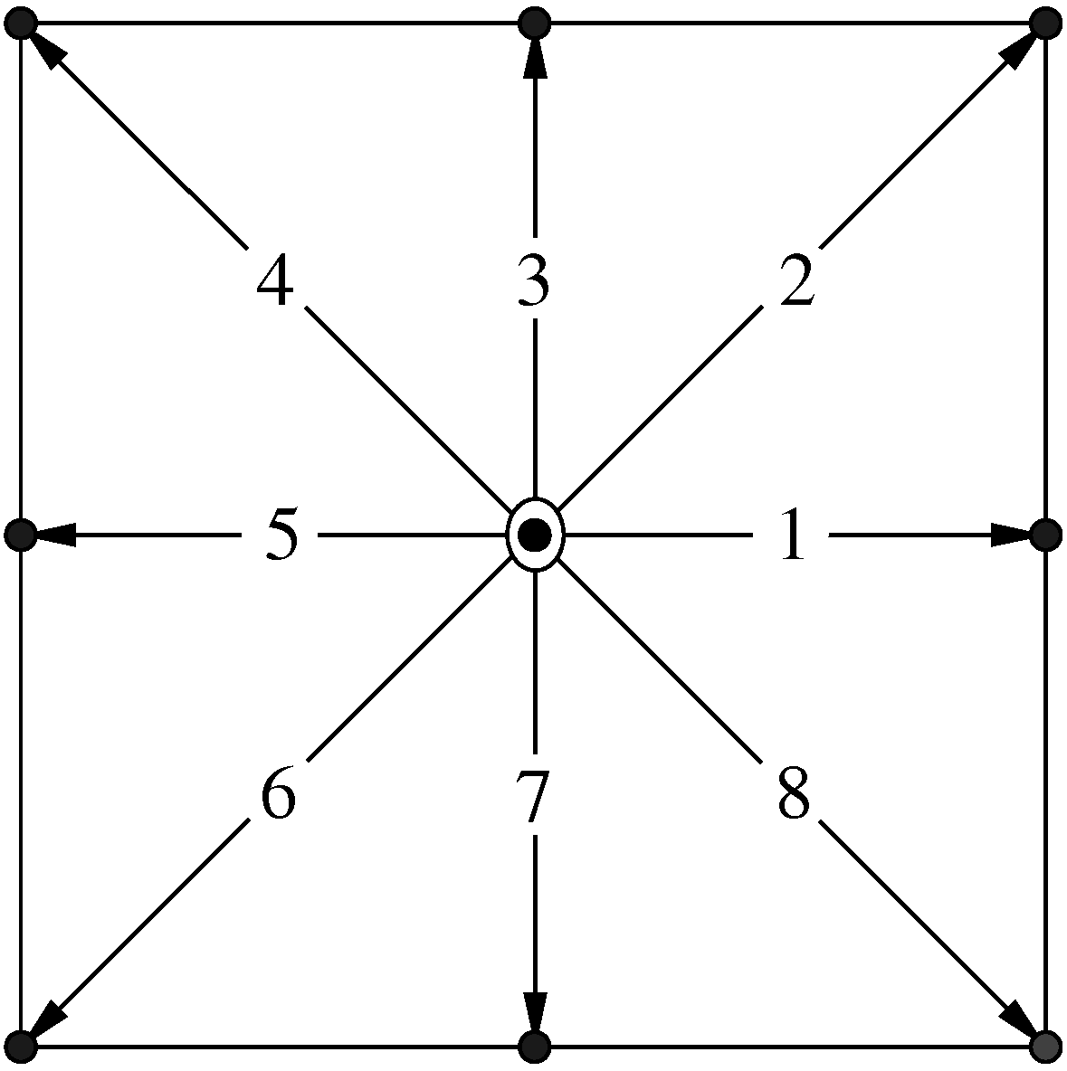
The enhanced lattice Boltzmann equation for the shallow water Equations (1) and (2) (eLABSWE) is described and reported in [15,16]. The eLABSWE is developed on a 2D square lattice with nine particle velocities (D2Q9) shown in Figure 1 and reads

$$\begin{array}{ccc}& & f_{\alpha }(\mathbf{x}+{\mathbf{e}}_{\alpha }\delta t,t+\delta t)=f_{\alpha }(\mathbf{x},t)-\frac{1}{\tau }[f_{\alpha }(\mathbf{x},t)-f_{\alpha }^{eq}(\mathbf{x},t)]\hfill \\ & & -\frac{g\overline{h}}{e^2}{C}_{\alpha }[z_b(\mathbf{x}+{\mathbf{e}}_{\alpha }\delta t)-z_b\left(\mathbf{x}\right)]+\frac{\delta t}{e^2}{C}_{\alpha }{e}_{\alpha j}{F}_j,\hfill \end{array}$$

(7)

where $f_{\alpha }$ is the particle distribution function; $\mathbf{x}$ is the space vector defined by Cartesian coordinates, i.e., $\mathbf{x}=(x,y)$ in 2D space; t is the time; $\delta t$ is the time step; ${\mathbf{e}}_{\alpha }$ is the particle velocity vector; $e_{\alpha j}$ is the component of ${\mathbf{e}}_{\alpha }$ in $j^{th}$ direction; $e=\delta x/\delta t$ is the particle speed, $\delta x$ is the lattice size; $\tau$ is the single relaxation time [23]; $C_{\alpha }=1/3$ when $\alpha =1,3,5,7$ and $C_{\alpha }=1/12$ when $\alpha =2,4,6,8$ and $f_{\alpha }^{eq}$ is the local equilibrium distribution function defined as

$$f_{\alpha }^{eq}=\left\{\begin{array}{cc}h\left(1-\frac{5gh}{6e^2}-\frac{2u_i{u}_i}{3e^2}\right),\hfill & \hfill \alpha =0,\\ {\lambda }_{\alpha }h\left(\frac{gh}{6e^2}+\frac{e_{\alpha i}{u}_i}{3e^2}+\frac{e_{\alpha i}{e}_{\alpha j}{u}_i{u}_j}{2e^4}-\frac{u_i{u}_i}{6e^2}\right),\hfill & \hfill \alpha \ne 0,\end{array}\right.$$

(8)

in which ${\lambda }_{\alpha }=1$ when $\alpha =1,3,5,7$ and ${\lambda }_{\alpha }=1/4$ when $\alpha =2,4,6,8$; and $\overline{h}$ is defined by

$$\overline{h}=0.5[h(\mathbf{x}+{\mathbf{e}}_{\alpha }\delta t,t+\delta t)+h(\mathbf{x},t)],$$

(9)

which is in an implicit form for $\overline{h}$ and reduces efficiency in the model. Although such implicitness can be eliminated by using the method by He et al. [24], it is founded that the use of a semi-implicit form, $\overline{h}=0.5[h(\mathbf{x}+{\mathbf{e}}_{\alpha }\delta t,t)+h(\mathbf{x},t)]$, is explicit, efficient and able to produce accurate solutions, which is preferred in practice for efficient simulations.

The physical variables of water depth and velocity are calculated as

$$h=\sum _{\alpha }{f}_{\alpha },$$

(10)

and

$$u_i=\frac{1}{h}\sum _{\alpha }{e}_{\alpha i}{f}_{\alpha }.$$

(11)

The depth-averaged eddy viscosity in eLASWE is determined as

$$\nu =\frac{e^2\delta t}{6}(2\tau -1).$$

(12)

The solution procedure for the eLABSWE is as follows:

• Initialise water depth and velocity;
• Select suitable lattice size $\delta x$ and time step $\delta t$;
• Choose single relaxation time $\tau$ according to the stability condition;
• Calculate $f_{\alpha }^{eq}$ from Equation (8) using water depth and velocity;
• Compute the particle distribution function $f_{\alpha }$ via the lattice Boltzmann Equation (7);
• Update the depth and velocity using Equations (10) and (11);
• Apply the bounce-back scheme for no-slip boundary condition or implement others through conversion of physical variables into particle distribution functions;
• Repeat Step (4) until a solution is reached.

4. Macroscopic Lattice Boltzmann Method (MacLABSWE)

To formulate a new macroscopic lattice Boltzmann method for the shallow water equations through the macroscopic physical variables of water depth and velocity without calculating particle distribution functions, Equation (7) is rearranged as

$$\begin{array}{ccc}& & f_{\alpha }(\mathbf{x}+{\mathbf{e}}_{\alpha }\delta t,t+\delta t)=f_{\alpha }^{eq}(\mathbf{x},t)+\left(1-\frac{1}{\tau }\right)[f_{\alpha }(\mathbf{x},t)-f_{\alpha }^{eq}(\mathbf{x},t)]\hfill \\ & & -\frac{g\overline{h}}{e^2}{C}_{\alpha }[z_b(\mathbf{x}+{\mathbf{e}}_{\alpha }\delta t)-z_b\left(\mathbf{x}\right)]+\frac{\delta t}{e^2}{C}_{\alpha }{e}_{\alpha j}{F}_j,\hfill \end{array}$$

(13)

Taking ∑ Equation (13) and $\sum e_{\alpha i}$ Equation (13) yields

$$\begin{array}{ccc}\hfill & & \sum f_{\alpha }(\mathbf{x}+{\mathbf{e}}_{\alpha }\delta t,t+\delta t)=\sum f_{\alpha }^{eq}(\mathbf{x},t)\hfill \\ \hfill & & -\frac{g}{e^2}\sum C_{\alpha }\overline{h}[z_b(\mathbf{x}+{\mathbf{e}}_{\alpha }\delta t)-z_b\left(\mathbf{x}\right)]+\frac{\delta t}{e^2}\sum C_{\alpha }{e}_{\alpha j}{F}_j,\hfill \end{array}$$

(14)

and

$$\begin{array}{ccc}\hfill & & \sum e_{\alpha i}{f}_{\alpha }(\mathbf{x}+{\mathbf{e}}_{\alpha }\delta t,t+\delta t)=\sum e_{\alpha i}{f}_{\alpha }^{eq}(\mathbf{x},t)\hfill \\ \hfill & & -\frac{g}{e^2}\sum C_{\alpha }{e}_{\alpha i}\overline{h}[z_b(\mathbf{x}+{\mathbf{e}}_{\alpha }\delta t)-z_b\left(\mathbf{x}\right)]+\frac{\delta t}{e^2}\sum C_{\alpha }{e}_{\alpha i}{e}_{\alpha j}{F}_j\hfill \end{array}$$

(15)

due to conservation of zeroth and first moments in the lattice Boltzmann method,

$$\sum f_{\alpha }(\mathbf{x},t)=\sum f_{\alpha }^{eq}(\mathbf{x},t),\sum e_{\alpha i}{f}_{\alpha }(\mathbf{x},t)=\sum e_{\alpha i}{f}_{\alpha }^{eq}(\mathbf{x},t).$$

(16)

The above Equations (14) and (15) can be rewritten as

$$\begin{array}{ccc}\hfill \sum f_{\alpha }(\mathbf{x},t)& =& \sum f_{\alpha }^{eq}(\mathbf{x}-{\mathbf{e}}_{\alpha }\delta t,t-\delta t)\hfill \\ & -& \frac{g}{e^2}\sum C_{\alpha }\overline{h}[z_b\left(\mathbf{x}\right)-z_b(\mathbf{x}-{\mathbf{e}}_{\alpha }\delta t)]+\frac{\delta t}{e^2}\sum C_{\alpha }{e}_{\alpha j}{F}_j,\hfill \end{array}$$

(17)

and

$$\begin{array}{ccc}\hfill \sum e_{\alpha i}{f}_{\alpha }(\mathbf{x},t)& =& \sum e_{\alpha i}{f}_{\alpha }^{eq}(\mathbf{x}-{\mathbf{e}}_{\alpha }\delta t,t-\delta t)+\frac{\delta t}{e^2}\sum C_{\alpha }{e}_{\alpha i}{e}_{\alpha j}{F}_j\hfill \\ & -& \frac{g}{e^2}\sum C_{\alpha }{e}_{\alpha i}\overline{h}[z_b\left(\mathbf{x}\right)-z_b(\mathbf{x}-{\mathbf{e}}_{\alpha }\delta t)].\hfill \end{array}$$

(18)

where

$$\overline{h}=0.5[h(\mathbf{x},t)+h(\mathbf{x}-{\mathbf{e}}_{\alpha }\delta t,t-\delta t)],$$

(19)

and the force term $F_j$, according to the centred scheme [7,25], can be evaluated at the midpoint between $(\mathbf{x}-{\mathbf{e}}_{\alpha }\delta t,t-\delta t)$ and $(\mathbf{x},t)$ for accurate solution [15,16] as

$$F_j=F_j\left(\mathbf{x}-\frac{1}{2}{\mathbf{e}}_{\alpha }\delta t,t-\frac{1}{2}\delta t\right).$$

(20)

By using Equations (10) and (11), the Equations (17) and (18) can be expressed as

$$\begin{array}{ccc}\hfill h(\mathbf{x},t)& =& \sum f_{\alpha }^{eq}(\mathbf{x}-{\mathbf{e}}_{\alpha }\delta t,t-\delta t)\hfill \\ \hfill & -& \frac{g}{e^2}\sum C_{\alpha }\overline{h}[z_b\left(\mathbf{x}\right)-z_b(\mathbf{x}-{\mathbf{e}}_{\alpha }\delta t)]+\frac{\delta t}{e^2}\sum C_{\alpha }{e}_{\alpha j}{F}_j\hfill \end{array}$$

(21)

and

$$\begin{array}{ccc}\hfill h(\mathbf{x},t)u_i(\mathbf{x},t)& =& \sum e_{\alpha i}{f}_{\alpha }^{eq}(\mathbf{x}-{\mathbf{e}}_{\alpha }\delta t,t-\delta t)+\frac{\delta t}{e^2}\sum C_{\alpha }{e}_{\alpha i}{e}_{\alpha j}{F}_j\hfill \\ & -& \frac{g}{e^2}\sum C_{\alpha }{e}_{\alpha i}\overline{h}[z_b\left(\mathbf{x}\right)-z_b(\mathbf{x}-{\mathbf{e}}_{\alpha }\delta t)].\hfill \end{array}$$

(22)

It can be seen from Equations (21) and (22) that the water depth and velocity are determined using the macroscopic physical variables through the local equilibrium distribution function without calculating the particle distribution function from Equation (7) that is required in Equations (10) and (11) for the depth and velocity in the eLABSWE. Equations (21) and (22) form the macroscopic lattice Boltzmann method for the shallow water equations (MacLABSWE). Clearly, it seems nowhere in the MacLABSWE to account for the eddy viscosity. This problem arises from the removal of the collision term in the lattice Boltzmann equation. As demonstrated in MacLAB [22], the problem is completely resolved through the discovery that the following formula

$$e=6\nu /\delta x,$$

(23)

is used for the particle speed e in the local equilibrium distribution function (8) for determining $f_{\alpha }^{eq}$ instead of using $e=\delta x/\delta t$ in the conventional lattice Boltzmann method. It will be shown in the recovery section that the eddy viscosity $\nu$ is already embedded in the model after Equation (23) is used.

The simulation procedure for MacLABSWE is as follows.

• Initialise water depth and velocity;
• Choose the lattice size $\delta x$ and determine the particle speed e from Equation (23);
• Calculate $f_{\alpha }^{eq}$ from Equation (8) using water depth and velocity;
• Update the depth and velocity using Equations (21) and (22);
• Only apply the boundary conditions when it is necessary;
• Repeat Step (3) until a solution is reached.

5. Recovery of the Shallow Water Equations

In this Section, we prove that the water depth and velocity calculated from Equations (21) and (22) satisfy the shallow water Equations (1) and (2). By realising that (A) Equations (21) and (22) are equivalent to Equations (17) and (18) due to the definitions of Equations (10) and (11), and (B) Equation (18) is obtained through $\sum e_{\alpha i}\times$ Equation (17), without loss of generality, we may start the derivation with Equation (17).

According to the Chapman–Enskog analysis, $f_{\alpha }$ can be expanded around local equilibrium distribution function as

$$f_{\alpha }=f_{\alpha }^{\left(0\right)}+f_{\alpha }^{\left(1\right)}\delta t+f_{\alpha }^{\left(2\right)}\delta t^2+\mathcal{O}\left(\delta t^3\right),$$

(24)

where $f_{\alpha }^{\left(0\right)}=f_{\alpha }^{eq}$ for conventional notation in the analysis. Substituting Equation (24) into Equation (17) leads to

$$\begin{array}{c}\hfill \sum [f_{\alpha }^{\left(0\right)}+f_{\alpha }^{\left(1\right)}\delta t+f_{\alpha }^{\left(2\right)}\delta t^2+\mathcal{O}\left(\delta t^3\right)]=\sum f_{\alpha }^{\left(0\right)}(\mathbf{x}-{\mathbf{e}}_{\alpha }\delta t,t-\delta t)\\ & & -\frac{g}{e^2}\sum C_{\alpha }\overline{h}[z_b\left(\mathbf{x}\right)-z_b(\mathbf{x}-{\mathbf{e}}_{\alpha }\delta t)]+\frac{\delta t}{e^2}\sum C_{\alpha }{e}_{\alpha j}{F}_j,\hfill \end{array}$$

(25)

Taking a Taylor expansion to the first term, $f_{\alpha }^{\left(0\right)}(\mathbf{x}-{\mathbf{e}}_{\alpha }\delta t,t-\delta t)$, on the right-hand side of above Equation (25) in time and space at point $(\mathbf{x},t)$ yields

$$\begin{array}{ccc}\hfill f_{\alpha }^{\left(0\right)}(\mathbf{x}-{\mathbf{e}}_{\alpha }\delta t,t-\delta t)& =& f_{\alpha }^{\left(0\right)}-\delta t\left(\frac{\partial }{\partial t}+e_{\alpha j}\frac{\partial }{\partial x_j}\right)f_{\alpha }^{\left(0\right)}\hfill \\ & +& \frac{1}{2}\delta t^2{\left(\frac{\partial }{\partial t}+e_{\alpha j}\frac{\partial }{\partial x_j}\right)}^2{f}_{\alpha }^{\left(0\right)}+\mathcal{O}\left(\delta t^3\right).\hfill \end{array}$$

(26)

Similarly, the second term on the right hand side of Equation (25) can also be expressed via the Taylor expansion,

$$\begin{array}{c}\hfill \frac{g{C}_{\alpha }}{e^2}\left[h-\frac{\delta t}{2}\left(\frac{\partial h}{\partial t}+e_{\alpha j}\frac{\partial h}{\partial x_j}\right)\right]\left(\delta t{e}_{\alpha j}\frac{\partial z_b}{\partial x_j}-\frac{\delta t^2}{2}{e}_{\alpha i}{e}_{\alpha j}\frac{{\partial }^2{z}_b}{\partial x_i\partial x_j}\right)+\mathcal{O}\left(\delta t^3\right),\end{array}$$

(27)

and the third term given by Equation (20) on the right hand side of Equation (25) can be written, via a Taylor expansion, as

$$\begin{array}{c}\hfill F_j\left(\mathbf{x}-\frac{1}{2}{\mathbf{e}}_{\alpha }\delta t,t-\frac{1}{2}\delta t\right)=F_j-\frac{\delta t}{2}\left(\frac{\partial }{\partial t}+e_{\alpha j}\frac{\partial }{\partial x_j}\right)F_j+\mathcal{O}\left(\delta t^2\right).\end{array}$$

(28)

After the substitution of Equations (26)–(28) into Equation (25), equating the coefficients of $\delta t$ results in, for the first-order $\delta t^1$,

$$\left(\frac{\partial }{\partial t}+e_{\alpha j}\frac{\partial }{\partial x_j}\right)f_{\alpha }^{\left(0\right)}=-f_{\alpha }^{\left(1\right)}-\frac{gh{C}_{\alpha }{e}_{\alpha j}}{e^2}\frac{\partial z_b}{\partial x_j}+\frac{C_{\alpha }{e}_{\alpha j}{F}_j}{e^2},$$

(29)

and for the second-order $\delta t^2$,

$$\begin{array}{ccc}& & -\frac{1}{2}{\left(\frac{\partial }{\partial t}+e_{\alpha j}\frac{\partial }{\partial x_j}\right)}^2{f}_{\alpha }^{\left(0\right)}=-f_{\alpha }^{\left(2\right)}+\frac{C_{\alpha }g{e}_{\alpha j}}{2e^2}\left(\frac{\partial h}{\partial t}+e_{\alpha i}\frac{\partial h}{\partial x_i}\right)\frac{\partial z_b}{\partial x_j}\hfill \\ & & +\frac{gh{C}_{\alpha }{e}_{\alpha i}{e}_{\alpha j}}{2e^2}\frac{{\partial }^2{z}_b}{\partial x_i\partial x_j}-\frac{C_{\alpha }{e}_{\alpha j}}{2e^2}\left(\frac{\partial F_j}{\partial t}+e_{\alpha i}\frac{\partial F_j}{\partial x_i}\right).\hfill \end{array}$$

(30)

Substitution of Equation (29) into Equation (30) gives

$$\frac{1}{2}\left(\frac{\partial }{\partial t}+e_{\alpha j}\frac{\partial }{\partial x_j}\right)f_{\alpha }^{\left(1\right)}=-f_{\alpha }^{\left(2\right)}.$$

(31)

Taking ∑ [(29) + $\delta t\times$ (31)] about $\alpha$ provides

$$\frac{\partial }{\partial t}\sum _{\alpha }{f}_{\alpha }^{\left(0\right)}+\frac{\partial }{\partial x_j}\sum _{\alpha }{e}_{\alpha j}{f}_{\alpha }^{\left(0\right)}=0.$$

(32)

which is in fact the second-order accurate continuity Equation (1) in local equilibrium distribution function, i.e., Equation (1) can be recovered by substitution of Equations (10), (11) and (16) into the Equation (32).

Taking ∑$e_{\alpha i}$ [(29) + $\delta t\times$ (31)] about $\alpha$ after mathematical manipulations yields

$$\begin{array}{ccc}& & \frac{\partial }{\partial t}\sum _{\alpha }{e}_{\alpha i}{f}_{\alpha }^{\left(0\right)}+\frac{\partial }{\partial x_j}\sum _{\alpha }{e}_{\alpha i}{e}_{\alpha j}{f}_{\alpha }^{\left(0\right)}+\frac{\delta t}{2}\frac{\partial }{\partial x_j}\sum _{\alpha }{e}_{\alpha i}{e}_{\alpha j}{f}_{\alpha }^{\left(1\right)}=-gh\frac{\partial z_b}{\partial x_i}+F_i.\hfill \end{array}$$

(33)

After using Equations (10), (11), (16) and (23), the above equation becomes the momentum Equation (2) with the eddy viscosity $\nu$, which is second-order accurate. Undoubtedly, the use of Equation (23) naturally embeds the eddy viscosity in the MacLABSWE without any treatment.

It should be pointed out that the shallow water equations have been recovered from the MacLABSWE and its proof is independent of the single relaxation time $\tau$, which is consistent with the development of the model in Section 4.

6. Unique Features and Main Limitation of the MacLABSWE

As the collision step is removed and only stream step or lattice size $\delta x$ is retained, the MacLABSWE becomes a precise lattice Boltzmann method and takes a minimal version of the method for shallow water flows. It may be stressed that the MacLABSWE is developed regardless of chosen value for the single relaxation time $\tau$, i.e., there is no assumption of setting $\tau =1$. The main features and limitation of the model is described and discussed in this section.

6.1. Unique Features

• Only lattice size $\delta x$ is required: After a lattice size $\delta x$ is chosen, the MacLABSWE is ready to simulate a flow with an eddy viscosity $\nu$ as seen from the solution procedure in Section 4. This is because $(x_j-e_{\alpha j}\delta t)$ stands for a neighbouring lattice point; $f_{\alpha }^{eq}$ at time of $(t-\delta t)$ represents its known quantity at the current time; and the particle speed e is determined from Equation (23) for use in computation of $f_{\alpha }^{eq}$.
• There is no need to choose time step $\delta t$: the time step $\delta t$ is no longer an independent parameter and calculated as $\delta t=\delta x/e$, which is used to calculate time in simulations of unsteady flows, and has no effect on steady flows.
• It is unconditionally stable: The method is unconditionally stable as it shares the same valid condition as that for $f_{\alpha }^{eq}$, or the Mach number $M=U_c/e$ is much smaller than 1, which is the intrinsic restriction on the lattice Boltzmann method, where $U_c$ is a characteristic flow speed. The Mach number can also be expressed as a lattice Reynolds number of $R_{le}=U_c\delta x/\nu$ via Equation (23). In practice, it is found that the model is stable if $R_{le}=U_m\delta x/\nu <1$ where $U_m$ is the maximum flow speed and is used as the characteristic flow speed.
• Physical variables are directly implemented as boundary conditions: As only macroscopic physical variables such as water depth and velocity are required, they are directly retained as boundary conditions with a minimum memory requirement at lower computational cost. At the same time, the most efficeint bounce-back scheme can be implemented as that in the standard lattice Botlzmann method if it is required, e.g., if the water depth is unknown and no-slip boundary condition is applied at south boundary for a straight channel, $f_2^{eq},f_3^{eq},f_4^{eq}$ in Equation (21) are unknown and they can be determined as $f_2^{eq}=f_6^{eq},f_3^{eq}=f_7^{eq},f_4^{eq}=f_8^{eq}$ using the bounce-back scheme for no-slip boundary condition, after which the water depth can be determined from Equation (21) and in this case Equation (22) is no longer required for calculation of velocity as the initial zero velocity will retain as no-slip boundary condition there.
• It is more efficient and needs less memory: compared to the eLABSWE [15,16], the proposed model is more efficient and needs less computer storage because for each time step in the eLABSWE, (1) calculations of particle distribution function $f_{\alpha }$ needs both additional computational cost and computer storage, and (2) conversion of physical variables into particle distribution function also needs additional computational cost for boundary conditions.
• It is an automatic simulator: All above features make the MacLABSWE an automatic simulator without tuning other simulation parameters for modelling a large flow system when a super-fast computer, such as a quantum computer, becomes available in the future.

6.2. Main Limitation

The only limitation of the proposed model is that, for a very small eddy viscosity or very high speed flow, the chosen lattice size after satisfying $R_{le}<1$ may turn out to generate very large lattice points (Lattice points, e.g., for one dimension with length of L is calculated as $N_L=L/\delta x$ and $N_L$ is the lattice points); if the total of lattice points is too big such that the demanding computations are beyond the current power of a computer, the simulation cannot be carried out. Such difficulties may be solved or relaxed through parallel computing using computer techniques such as GPU processors and multiple servers, and will be largely or completely removed using a quantum computer when it becomes available.

7. Validation

In order to verify the described model, three numerical tests typical of shallow water flows are presented. The SI Units are used for the physical variables in the following numerical simulations.

7.1. 1D Tidal Flow

First of all, a tidal flow over an irregular bed is predicted, which is a common flow problem in coastal engineering. The bed is defined with data listed in

Table 1. Bed elevation $z_b$ for irregular bed.

Horizontal distance		$x\left(m\right)$	0	50	100	150	250	300	350	400
Bed elevation		$z_b\left(m\right)$	0	0	2.5	5	5	3	5	5
$x\left(m\right)$	425	435	450	475	500	505	530	550	565	575
$z_b\left(m\right)$	7.5	8	9	9	9.1	9	9	6	5.5	5.5
$x\left(m\right)$	600	650	700	750	800	820	900	950	1000	1500
$z_b\left(m\right)$	5	4	3	3	2.3	2	1.2	0.4	0	0

. Here, we consider a 1D problem with the initial and boundary conditions of

$$h(x,0)=16-z_b\left(x\right),$$

(34)

$$u_x(x,0)=0$$

(35)

and

$$h(0,t)=20-4sin\left[\pi \left(\frac{4t}{86,400}+\frac{1}{2}\right)\right],$$

(36)

$$u_x(1500,t)=0.$$

(37)

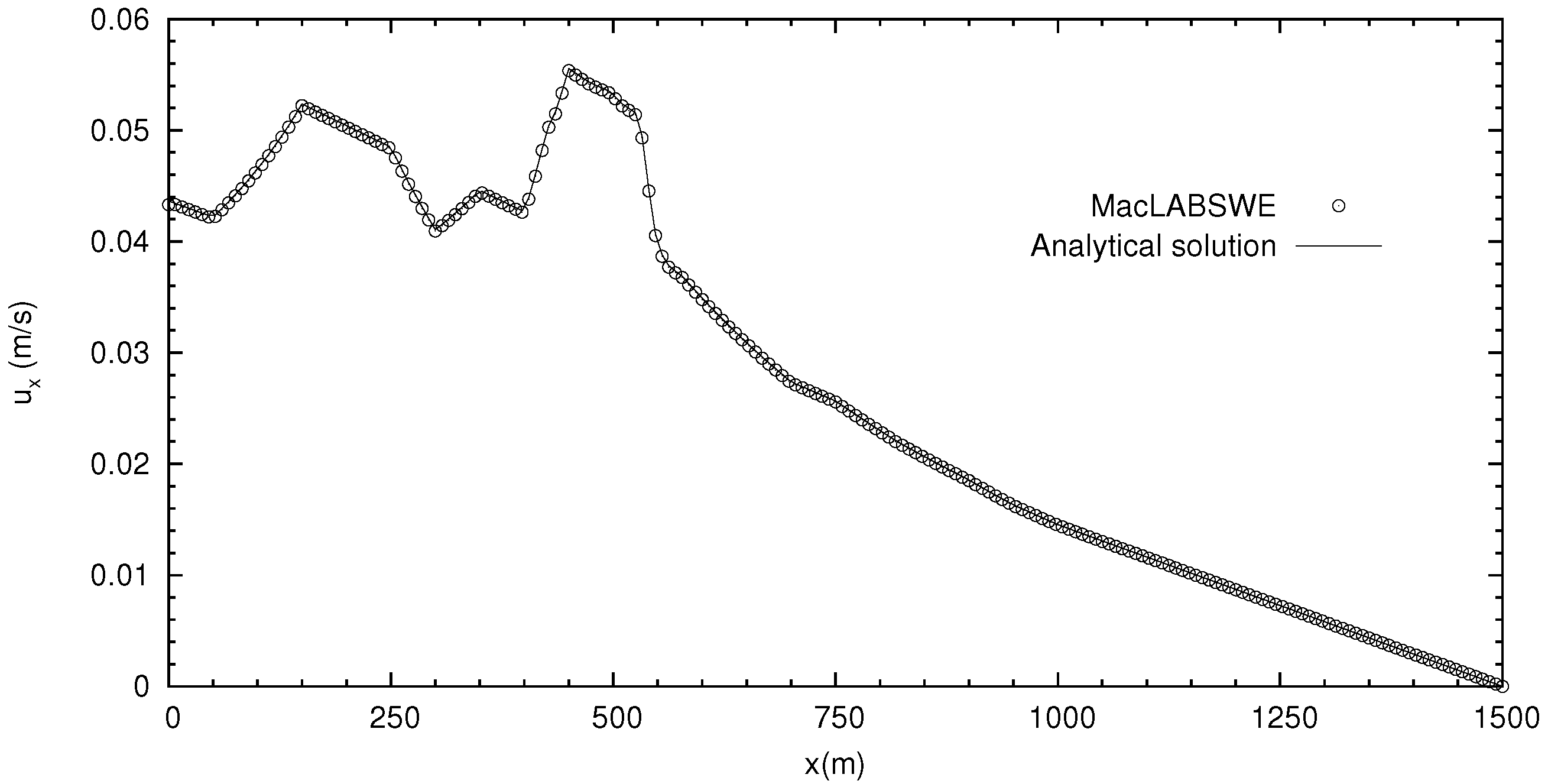
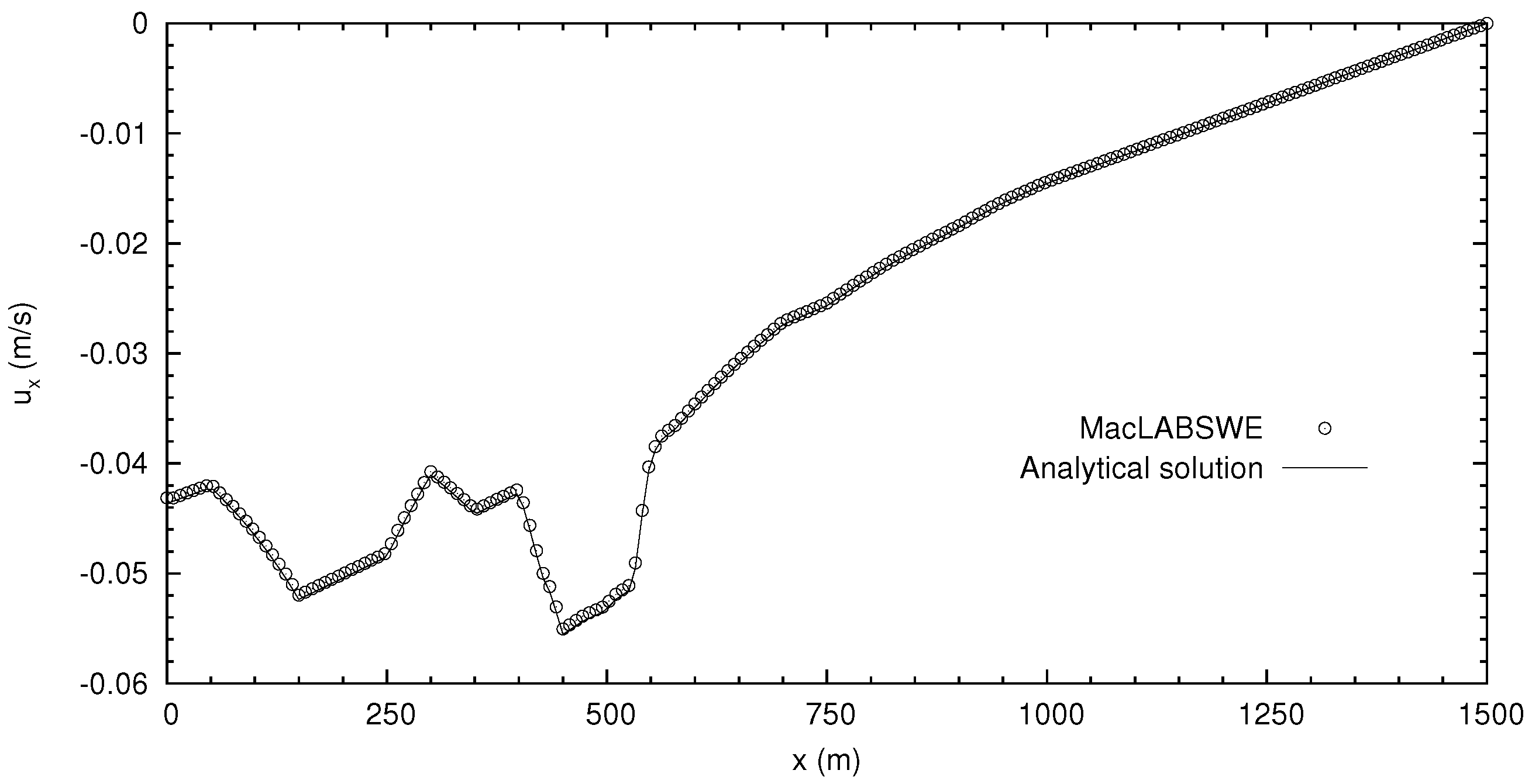
In the simulation, $\delta x=7.5$ m or 200 lattices are used with eddy viscosity of $\nu =31.25$ m${}^2$/s for same computational parameters used in [15]. This is an unsteady flow. Two numerical results at $t=$ 10,800 s and $t=$ 32,400 s corresponding to the half-risen tidal flow with maximum positive velocities and to the half-ebb tidal flow with maximum negative velocities are compared with the analytical solutions [26] and depicted in Figure 2 and Figure 3, respectively. The maximum relative errors are less than 0.005% for the water level, less than 0.05% for velocity larger than 0.002 m/s, and less than 0.3% for smaller velocity, revealing excellent agreements. After compared with the results using eLABSWE [15,16], it is revealed that the two models effectively predict the similar accurate results up to machine-accuracy of a computer. However, the current model is more efficient and needs less computer storage to generate the solutions.

7.2. 2D Wind-Driven Circulation

Secondly, we consider a wind-driven circulation in a lake, which may generate a complex flow phenomenon depending on the bed topography of a lake and the wind speed. In this test, a uniform wind shear stress is applied to the shallow water in a circular basin with the bed topography defined by the still water depth H,

$$H(x,y)=\frac{1}{1.3}\left(\frac{1}{2}+\sqrt{\frac{1}{2}-\frac{\sqrt{x^2+y^2}}{386.4}}\right),$$

(38)

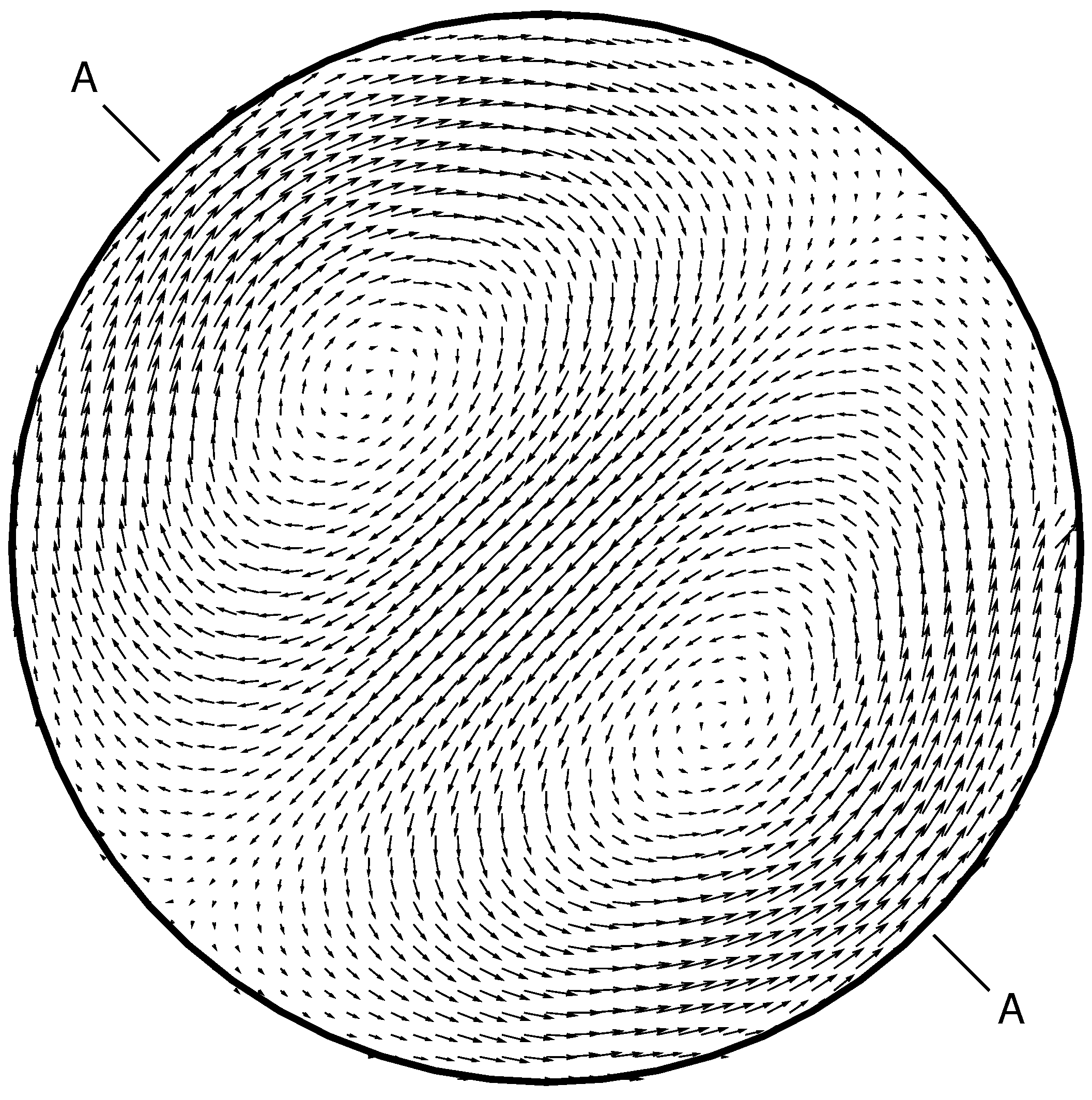
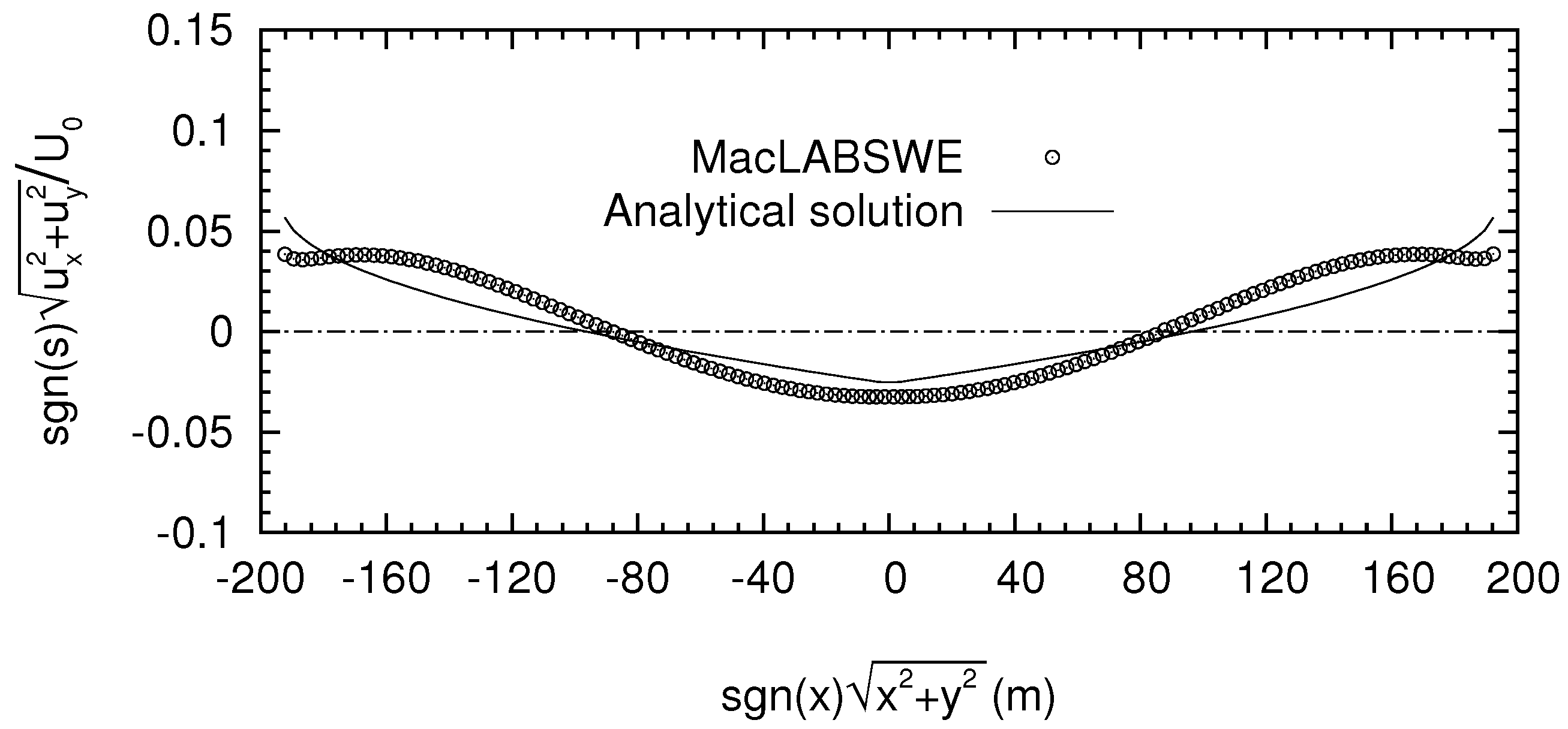
from which, the bed level can be determined as $z_b(x,y)=H(0,0)-H(x,y)$. The same dish-shaped basin is also used by Rogers et al. [27] to test a Godunov-type method. Initially, the water in the basin is still and then a uniform wind speed of $u_w=5$ m/s blows from southwest to northeast, at which wind shear stress is calculated from Equation (4). Its steady flow consists of two relatively strong counter-rotating gyres with flow in the deeper water against the direction of the wind, exhibiting complex flow phenomenon. In the numerical computation, $\delta x=2$ or $200\times 200$ lattices are used with eddy viscosity of $\nu$ = 5.33 m${}^2$/s. After the steady solution is obtained, the flow field is shown in Figure 4 and the normalised resultant velocities at cross section A-A are compared with the analytical solution [28] in Figure 5, exhibiting similar agreement to that by Zhou and Liu using eLABSWE [16] for the same test. Although there is discrepancy between the numerical prediction and the analytical solution, such agreement is reasonable due to the fact that the assumptions of both the rigid-lid approximation for the water surface and a parabolic distribution for the eddy viscosity were used in the analytical solution.

7.3. Flow over a 2D Hump

Finally, a steady shallow water flow over a 2D hump is investigated. The 2D hump is defined as

$$z_b(x,y)=\left\{\begin{array}{cc}\psi (x,y),\hfill & \hfill \mathrm{if}\hspace{0.17em}(x,y)\in \Omega ,\\ 0,\hfill & \hfill \mathrm{otherwise},\end{array}\right.$$

(39)

where $\Omega =[300,500]\times [400,600]$ and

$$\psi (x,y)={sin}^2\left(\frac{\pi (x-300)}{200}\right){sin}^2\left(\frac{\pi (y-400)}{200}\right).$$

(40)

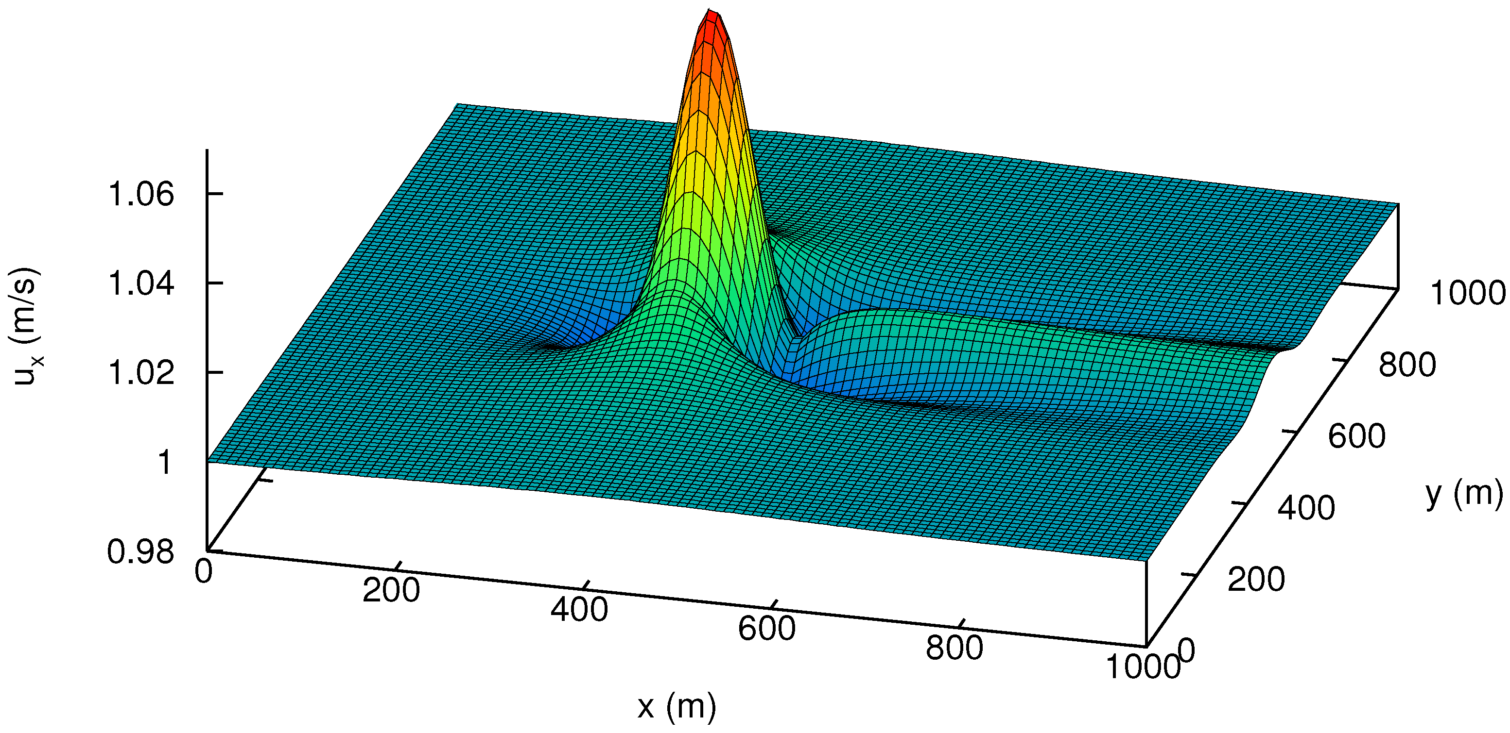
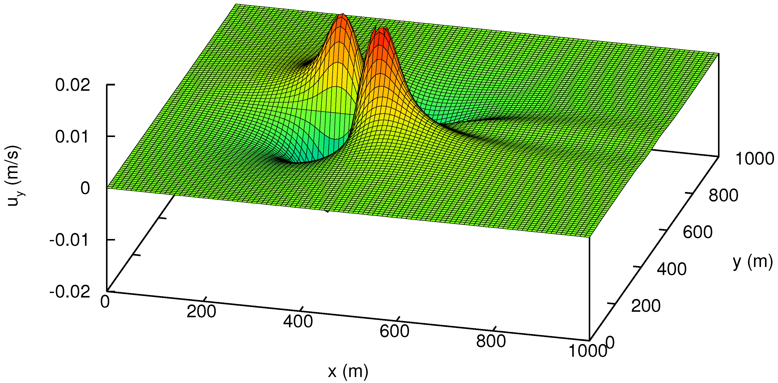
The flow conditions are: discharge per unit width is $q=10$ m${}^2$/s; water depth is $h=10$ m at the outflow boundary and the channel is 1000 m long and 1000 m wide. This is the same test as that used by researchers in validation of numerical methods [29,30,31] for sediment transport under shallow water flows. Here, only steady flow over the fixed bed without sediment transport is simulated as prediction of correct flow plays an essential role in the determination of bed evolution, and hence it is a suitable test for the proposed scheme. We use $\delta x=5$ or $200\times 200$ lattices in the simulation. After the steady solution is obtained, the velocities $u_x$ and $u_y$ are shown in Figure 6 and Figure 7, respectively, demonstrating good agreements with those obtained using high-resolution Godunov-type numerical methods [29,30,31]. The results are also compared to that using the eLABSWE and again show similar accuracy.

8. Conclusions

The paper presents a novel macroscopic lattice Boltzmann method for the shallow water equations (MacLABSWE). The collision step is removed and the model is completely determined by the lattice size only, creating a minimal version of the lattice Boltzmann method, MacLABSWE. This changes the standard view of two integral steps of streaming and collision in the conventional lattice Boltzmann method. The shallow water equations are recovered from the MacLABSWE to ensure that the calculated water depth and velocities from the mode are the solutions to the shallow water equations. The derivation of the model and the recovery of the flow equations are independent of the single relaxation time $\tau$ and consistent with each other. Steady and unsteady numerical tests have shown that the method can provide accurate solutions. The main conclusions are

• The method is unconditionally stable, which shares the same validation as that of the local equilibrium distribution function. This takes the research on the method into a new era in which future work may focus on improving the accuracy of or formulating a new local equilibrium distribution function.
• The model depends on physical variables only and they are directly applied as boundary condition without converting them to their corresponding distribution functions, which not only save computational storage at lower computational cost but also achieve an exact no-slip boundary condition unlike the use of the first or second order-accurate bounce-back scheme.
• The MacLABSWE is an automatic model for water flows once a lattice size is chosen. It is an ideal model for simulation of any scale flows to achieve an ultimate goal of generating real-time predictions for solving challenging flow problems such as weather forecast and flooding when a super-fast computer such as a quantum computer becomes available in the future.
• It is discovered that the use of Equation (23) for the particle speed e in the local equilibrium distribution function naturally embeds the eddy viscosity in the MacLABSWE without any treatment.
• The model preserves the simple arithmetic calculations of the lattice Boltzmann method at the full advantages of the conventional lattice Boltzann method. The most efficient bounce-back scheme can be applied straightforwardly, if it is necessary.
• The solution procedure involves two fewer steps compared to eLABSWE and the conventional lattice Boltzmann method, making the model more efficient.

References

- Vreugdenhil, C.B. Numerical Methods for Shallow-Water Flow; Kluwer Academic Publishers: Dordrecht, The Netherland, 1994. [Google Scholar]
- Alcrudo, A.; Garcia-Navarro, P. A High Resolution Godunov-Type Scheme in Finite Volumes for the 2D Shallow Water Equations. Int. J. Numer. Methods Fluids 1993, 16, 489–505. [Google Scholar] [CrossRef]
- Casulli, V. Semi-implicit Finite Difference Methods for the Two-dimensional Shallow Water Equations. J. Comput. Phys. 1990, 86, 56–74. [Google Scholar] [CrossRef]
- Borthwick, A.G.L.; Akponasa, G.A. Reservoir flow prediction by contravariant shallow water equations. J. Hydr. Eng. Div. ASCE 1997, 123, 432–439. [Google Scholar] [CrossRef]
- Yulistiyanto, B.; Zech, Y.; Graf, W.H. Flow around a cylinder: Shallow-water modeling with diffusion-dispersion. J. Hydraul. Eng. ASCE 1998, 124, 419–429. [Google Scholar] [CrossRef]
- Hu, K.; Mingham, C.G.; Causon, D.M. Numerical simulation of wave overtopping of coastal structures using the non-linear shallow water equations. Coast. Eng. 2000, 41, 433–465. [Google Scholar] [CrossRef]
- Zhou, J.G. Lattice Boltzmann Methods for Shallow Water Flows; Springer: Berlin, Germany, 2004. [Google Scholar]
- Zhou, J.G. Velocity-Depth Coupling in Shallow Water Flows. J. Hydr. Eng. ASCE 1995, 121, 717–724. [Google Scholar] [CrossRef]
- Zhou, J.G.; Causon, D.M.; Mingham, C.G.; Ingram, D.M. The surface gradient method for the treatment of source terms in the shallow-water equations. J. Comput. Phys. 2001, 168, 1–25. [Google Scholar] [CrossRef]
- Zhou, J.G. A lattice Boltzmann model for the shallow water equations. Comput. Methods Appl. Mech. Eng. 2002, 191, 3527–3539. [Google Scholar] [CrossRef]
- Swift, M.R.; Osborn, W.R.; Yeomans, J.M. Lattice Boltzmann Simulation of Nonideal Fluids. Phys. Rev. Lett. 1995, 75, 830–833. [Google Scholar] [CrossRef] [Green Version]
- Spaid, M.A.A.; Phelan, F.R., Jr. Lattice Boltzmann method for modeling microscale flow in fibrous porous media. Phys. Fluids 1997, 9, 2468–2474. [Google Scholar] [CrossRef]
- Zhou, J.G. A lattice Boltzmann Model for Groundwater Flows. Int. J. Mod. Phys. C 2007, 18, 973–991. [Google Scholar] [CrossRef]
- Zhou, J.G. Lattice Boltzmann morphodynamic model. J. Comput. Phys. 2014, 270, 255–264. [Google Scholar] [CrossRef]
- Zhou, J.G. Enhancement of the LABSWE for shallow water flows. J. Comput. Phys. 2011, 230, 394–401. [Google Scholar] [CrossRef]
- Zhou, J.G.; Liu, H. Determination of bed elevation in the enhanced lattice Boltzmann method for the shallow-water equations. Phys. Rev. E 2013, 88, 023302. [Google Scholar] [CrossRef]
- Liu, H.; Zhou, J.G.; Burrows, R. Lattice Boltzmann model for shallow water flows in curved and meandering channels. Int. J. Comput. Fluid Dyn. 2009, 23, 209–220. [Google Scholar] [CrossRef]
- Liu, H.; Zhou, J.G.; Burrows, R. Multi-block lattice Boltzmann simulations of subcritical flow in open channel junctions. Comput. Fluids 2009, 38, 1108–1117. [Google Scholar] [CrossRef]
- Liu, H.; Zhou, J.G.; Burrows, R. Numerical modelling of turbulent compound channel flow using the lattice Boltzmann method. Int. J. Numer. Methods Fluids 2009, 59, 753–765. [Google Scholar] [CrossRef]
- Liu, H.; Zhou, J.G.; Li, M.; Zhao, Y. Multi-block lattice Boltzmann simulations of solute transport in shallow water flows. Adv. Water Resour. 2013, 58, 24–40. [Google Scholar] [CrossRef]
- Ladd, A.J. Numerical simulations of particulate suspensions via a discretized Boltzmann equation. Part 1.Theoretical foundation. J. Fluid Mech. 1994, 285, 285–309. [Google Scholar] [CrossRef] [Green Version]
- Zhou, J.G. Macroscopic Lattice Boltzmann Method. Water 2021, 13, 61. [Google Scholar] [CrossRef]
- Bhatnagar, P.L.; Gross, E.P.; Krook, M. A model for collision processes in gases. I: Small amplitude processes in charged and neutral one-component system. Phys. Rev. 1954, 94, 511–525. [Google Scholar] [CrossRef]
- He, X.; Chen, S.; Doolen, G.D. A Novel Thermal Model for the Lattice Boltzmann Method in Incompressible Limit. J. Comput. Phys. 1998, 146, 282–300. [Google Scholar] [CrossRef]
- Zhou, J.G. Axisymmetric lattice Boltzmann method revised. Phys. Rev. E 2011, 84, 036704. [Google Scholar] [CrossRef] [PubMed]
- Bermudez, A.; Vázquez, M.E. Upwind Methods for Hyperbolic Conservation Laws with Source Terms. Comput. Fluids 1994, 23, 1049–1071. [Google Scholar] [CrossRef]
- Rogers, B.; Fujihara, M.; Borthwick, A.G.L. Adaptive Q-tree Godunov-Type Scheme for Shallow Water Equations. Int. J. Numer. Methods Fluids 2001, 35, 247–280. [Google Scholar] [CrossRef]
- Kranenburg, C. Wind-driven chaotic advection in a shallow model lake. J. Hydr. Res. 1992, 30, 29–46. [Google Scholar] [CrossRef]
- Benkhaldoun, F.; Sahmim, S.; Seaïd, M. A two-dimensional finite volume morphodynamic model on unstructured triangular grids. Int. J. Numer. Methods Fluids 2010, 63, 1296–1327. [Google Scholar] [CrossRef]
- Huang, J.; Borthwick, A.G.L.; Soulsby, R.L. Adaptive Quadtree Simulation of Sediment Transport. Proc. Inst. Civ. Eng. J. Eng. Comput. Mech. 2010, 163, 101–110. [Google Scholar] [CrossRef] [Green Version]
- Hudson, J.; Sweby, P.K. A high-resolution scheme for the equations governing 2D bed-load sediment transport. Int. J. Numer. Methods Fluids 2005, 47, 1085–1091. [Google Scholar] [CrossRef]
Figure 1.
Two-dimensional square lattice for nine-particle velocities, which are labelled by Numbers 1–8 for directions and 0 for still particle (D2Q9).
Figure 2.
Comparison of velocity at 10,800 s when flow is in the half-risen tide with maximum positive velocities for 1D tidal flow.
Figure 3.
Comparison of velocity at 32,400 s when the flow is in the half-ebb tide with maximum negative velocities for 1D tidal flow.
Figure 4.
Flow field for wind-driven flow, showing well-developed counter-rotating gyres with flow in the deeper water against the direction of the wind.
Figure 5.
Comparison of the resultant velocities along cross-section A-A (see Figure 4) with the analytical solution [28], where and .
Figure 6.
Velocity distribution for a steady flow over a 2D bump.
Figure 7.