
Multi-Isotope Characterization of Water in the Water Supply System of the City of Ljubljana, Slovenia
by
 , ,
, ,
Klara Nagode
1,2,* ,
,
Tjaša Kanduč
1,
Branka Bračič Železnik
3,
Brigita Jamnik
3 and
Polona Vreča
1 1
Department of Environmental Sciences, Jožef Stefan Institute, Jamova cesta 39, 1000 Ljubljana, Slovenia
2
Jožef Stefan International Postgraduate School, Jamova cesta 39, 1000 Ljubljana, Slovenia
3
JP VOKA SNAGA d.o.o., Vodovodna cesta 90, 1000 Ljubljana, Slovenia
*
Author to whom correspondence should be addressed.
Water 2022, 14(13), 2064; https://doi.org/10.3390/w14132064
Submission received: 10 May 2022
/
Revised: 6 June 2022
/
Accepted: 10 June 2022
/
Published: 28 June 2022
(This article belongs to the Special Issue Use of Water Isotopes in Hydrological Processes II)
Abstract
:Urban water supply systems (WSS) are complex and challenging to manage since the properties of water in the WSS change from source to the end user over time. However, understanding these changes requires a more profound knowledge of the WSS. This study describes the urban water cycle within the WSS of Ljubljana, Slovenia, where different water parameters such as temperature, electrical conductivity, total alkalinity, δ2H, δ18O, and δ13CDIC were monitored from September to November 2018. Altogether 108 samples were collected, including from the source (3) and at different levels of the WSS: wells (41), joint exits from water pumping stations (7), reservoirs (22), water treatment locations (2), drinking fountains (13), taps (19) and wastewater system (1). The data show that although the ranges of δ2H and δ18O values were small, each well is represented by a unique fingerprint when considering additional parameters. A statistically significant difference was observed between sampling months, and temperature and most parameters showed higher variability within the wells than across the WSS, suggesting a more unified WSS. Finally, based on δ13CDIC values, a distinction could be made between river/groundwater interactions within the WSS and between shallower and deeper wells and their distance from the river bank.
1. Introduction
Urban water supply systems (WSS) are complex and dynamic and are composed of multiple interdependent components, i.e., water resources, storage units, pumping stations, reservoirs, transfer lines, and channels and, like any other system, they are prone to physical disruption and pollution [1]. Rapid growth in populations and urbanization has resulted in a dramatic increase in water usage, putting considerable strain on existing WSS, which cannot adequately adapt to accommodate the new level of demand [2]. As a result, in many countries, WSS might become deficient and poorly understood [1]. The allocation and management of water sources are also increasingly challenging due to environmental factors such as pollution and climate change [3,4]. Therefore, what is needed is a multidisciplinary approach to address such issues. In this respect, stable isotopes can be used to complement other hydro-chemical information about the system [5]. The application of water isotopes (δ18O and δ2H) is based on the assumption that the isotopic signature of water is present with unique values that change with time and space [6,7]. This conservative behavior allows new insights into the mechanisms, pathways, and interactions of water bodies in urban systems [4,8]. Moreover, the isotopic composition of carbon in dissolved inorganic carbon (δ13CDIC) is important in deciphering the origin of carbon in the water system since HCO3− is the primary species leaching from carbonate rocks [9].
Applying the stable isotope approach in urban water settings has increased in recent years and, as a consequence, yielded promising results. For example, stable isotope values of tap water were used to identify and quantitatively characterize the water sources, water management practices, and structure of different WSS and quantify the effects of climate variability [3,4,8,10,11]. In addition, Leslie and others [12] used the stable isotope values in municipal water to delineate the residence time of water in a WSS based on the lag between precipitation and residential tap water over time. In most cases, these systems are investigated by sampling sources and tap water, and so far, only Sánchez-Murillo et al. [11] have investigated other engineering features, i.e., storage units or tanks, transfer lines/pumping units, over a short period (over 2–3 days).
The provision of water for domestic supply in urban areas is complex and usually involves many sources (i.e., precipitation, surface water, and groundwater). The WSS for Ljubljana, the capital city of Slovenia, is no exception and is still in use today despite being designed more than 100 years ago. The main source of drinking water for the city is the groundwater from the Ljubljansko polje aquifer, although some of it derives from the Ljubljansko barje aquifer in the southern part of Ljubljana [13]. So far, only short−term investigations of the WSS have been performed that focus on groundwater dynamics, modeling [14,15] and chemical and isotope investigations to characterize the aquifers, sources, and water interactions for the aquifers’ water supply [14,16,17,18,19,20]. Despite the usefulness of stable isotopes (H, O, C) for managing water resources, Slovenian regulation does not require the analysis of stable isotopes in drinking water. Consequently, as concluded by a thorough review of past investigations [19], no systematic investigation of the isotope composition of drinking water in Ljubljana from “source to tap” has been performed.
In this paper, the results of a short, preliminary investigation of Ljubljana’s WSS from well to tap are presented. The aim was to perform a systematic assessment of the use of stable isotopes and other physicochemical properties to evaluate water sources, pathways, and interactions to improve water supply management. More specifically, the paper addresses the following research questions: Can isotopic signatures characterize different urban water cycle components? Can the unique isotopic signatures be used to define better the sources, pathways, and interactions between water bodies (e.g., groundwater and river water) in urban environments and WSS? The data provided also represents an initial database for future comparison of the WSS.
2. Materials and Methods
2.1. Site Description
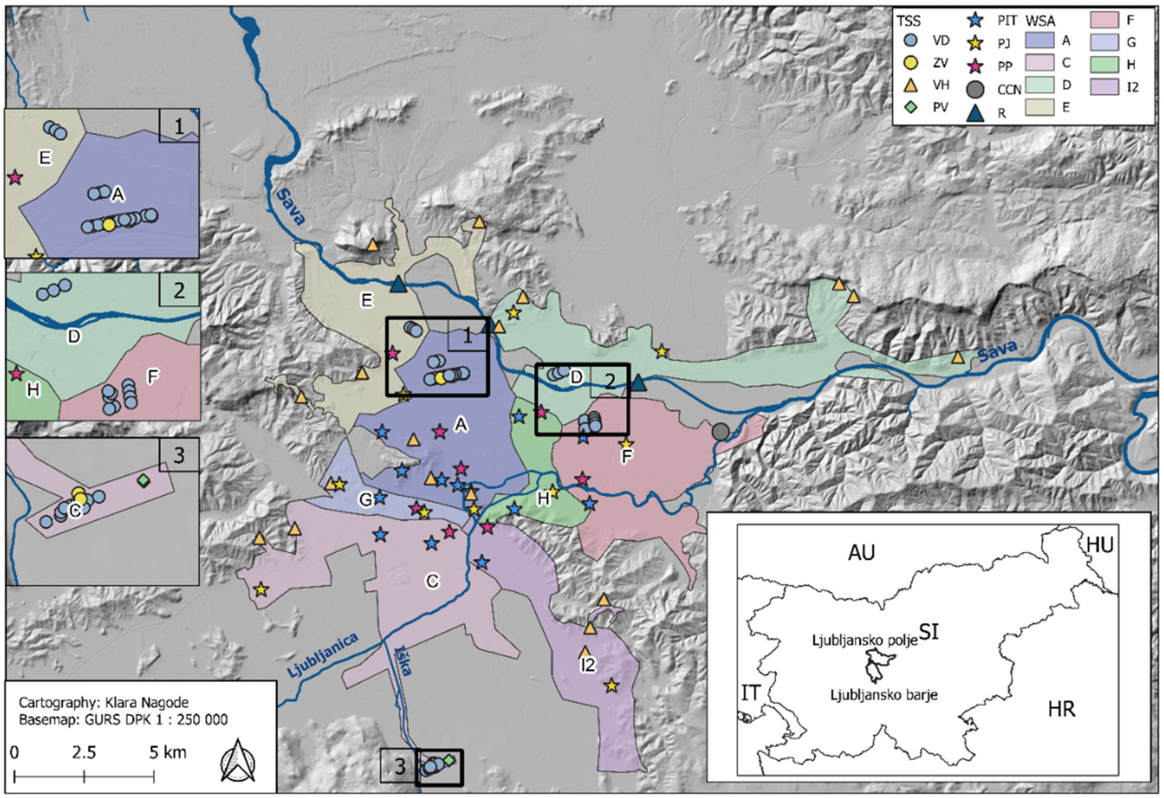
Sampling was performed in two sections of the Ljubljana basin: the Ljubljansko polje (LP), an unconfined alluvial aquifer in the northern part of the and the Ljubljansko barje (LB), a confined aquifer in the southern part of the basin (Figure 1) [15]. A detailed description of the aquifers is given in [19,21]. The aquifers are separated by the hills Golovec, Grajski hrib and Rožnik. The hills and the bedrock of the LP are composed of impermeable Permian and Carboniferous schist, claystone, and sandstone [22]. It was formed by tectonic subsidence and filled with Pleistocene and Holocene alluvial sediments of up to 120 m in thickness. The aquifer is generally recharged from infiltration of precipitation, the River Sava (north-western part) and via lateral inflow from the Ljubljansko barje multi-aquifer system [15]. The Ljubljansko barje is a depression formed by tectonic subsidence and filled by alluvial and lacustrine sediments during the Pleistocene and Holocene epochs. The heterogeneity of sediments means that the hydrogeological conditions in the LB are more complicated than in the LP [16,22].
The largest water company in Slovenia in terms of users is the Public Water Utility JP VOKA SNAGA d.o.o. Drinking water has been supplied to users in Ljubljana since 1890. Currently, the majority of the groundwater is extracted from the Kleče (A) wellfield at LP, while the contribution of other wellfields at LP; Hrastje (B), Jarški prod (D) and Šentvid (E) and from LB from Brest (C) is lower (Figure 1). Water is pumped from 44 wells and is distributed through more than 1100 km of supply network [23], and it takes a few hours for water from the wellfield to reach the end-user. Well depths typically range from 30 to 105 m below the surface, with pumping rates from 15 to 92 L/s. The perforated screens in the pumping wells vary at LP from 200 to 290 m a.s.l. Their elevation is between 281.4 and 310.0 m a.s.l. In the LB, the screens are located between 290 m and 270 m a.s.l. for shallow wells and 270 to 195 m a.s.l. for deeper wells (e.g., Brest 2a and Brest 4a). Their elevation is between 299.5 and 301.9 m a.s.l. (Supplementary Figure S1). In the central system, certain settlements are continuously supplied with drinking water from a single wellfield (A, C, D, and E), while others are supplied from two or more wellfields: F, G, H, and I2 (Figure 1) [20]. In Ljubljana, WSS also includes other components: joint exits from water pumping stations (ZV), reservoirs (VH), water treatment locations (PV), drinking water fountains (PIT) and taps in public buildings (PJ) and private buildings (PP).
2.2. Selection of Sampling Sites and Sampling
Based on the knowledge of the JP VOKA SNAGA d.o.o. personnel and previous investigations of the WSS, 97 sampling sites, which are used for the regular monitoring of drinking water, were selected for investigation (Figure 1). Sampling sites were selected according to (a) the type of sampling site (TSS) in the WSS and (b) the type of water supply area (WSA). Based on TSS, the initial selection included wells (VD, 44 samples), joint exits from water pumping stations (ZV; 7 samples), reservoirs (VH; 23 samples), water treatment locations (PV; 2 samples), drinking water fountains (PIT; 13 samples) and taps in public (PJ; 10 samples) and private buildings (PP; 8 samples). The sampling of the WSA initially included 4 main wellfields: Kleče (A; N = 35), Brest (C; N = 22), Jarški prod (D; N = 10) and Šentvid (E; N = 11) and four areas where water is mixed from two or three different WSA: Hrastje/Jarški prod (F; N = 5), Kleče/Brest (G; N = 5), Kleče/Hrastje/Jarški prod (H; N = 3) and Kleče/Hrastje/Brest (I2; N = 6). Wells from the Hrastje wellfield (B; N = 10) were also included, although it does not represent a unique WSA.
In order to cover the whole WSS, an additional three locations along the River Sava (R; locations Brod, Črnuče and Šentjakob) and at the outflow from a wastewater treatment plant (CČN) were selected. Data collection focused on a 3-month period between 6 September 2018 and 29 November 2018. Altogether, 8, 10 and 12 sampling campaigns were performed in September, October and November 2018, respectively. Samples at four sites were not collected, and one site (PJ) was sampled twice. The final collection of samples included sampling in VD (41), ZV (7), VH (22), PV (2), PIT (13), PJ (11) and PP (8). In total, 104 samples were collected at 103 locations. The majority of well samples (41) were collected in September, while eight samples from Kleče and six from Brest were collected in October and November 2018. In the field, temperature (T) and electrical conductivity (EC) measurements were collected, while pH, total alkalinity (TA), isotope composition of hydrogen (δ2H), oxygen (δ18O) and carbon in the dissolved inorganic carbon (δ13CDIC) were measured in the laboratory. Metadata and results are presented in [24]. Water samples from the various components of the WSS (93 sites in the WSS and at the outflow of CČN) were collected by JP VOKA SNAGA d.o.o., while the JSI team members and volunteers performed sampling at PP and two locations at PJ. From 2016 to 2018, daily air temperature and precipitation data were obtained from the Environmental Agency of the Republic of Slovenia for the station at Ljubljana–Bežigrad [25]. In addition, monthly composite precipitation samples were collected at Ljubljana-Reactor, where monitoring has been performed since 1981 [26,27,28].
2.3. In-Situ Measurements
Temperature (T) and electrical conductivity (EC) were determined together in-situ using an Ultrameter IITM 6PFCE (MIRON L Company, Carlsbad, CA, USA). The measurement accuracy was ±0.1 °C for T and ±1% for EC. However, T and EC were not measured for all tap water samples (10). Samples were collected using the following protocol: taps were opened for 5 min [11] before sampling to avoid stagnant water.
2.4. Analytical Procedures
2.4.1. Determination of Total Alkalinity (TA)
To determine the TA, each sample was passed through a 0.45 μm nylon filter into an HDPE bottle and kept refrigerated until analyzed. First, the pH was measured (SevenCompactTM pH/Ion S220, Mettler-Toledo 8603 Schwanzenbach, Switzerland, Rating 9–12 V, made by Mettler Toledo group). The TA was then measured by Gran titration [29] with a precision of ±1%. Sample repeatability was ±0.1 mM.
2.4.2. Determination of δ2H, δ18O and d-Excess
δ2H and δ18O values were determined according to [20]. The results are expressed using the standard δ notation (in‰):
δsample (‰) = (Rsample/Rstandard − 1) × 1000
Rsample and Rstandard are the isotope ratios (2H/1H and 18O/16O) of a heavy isotope to a light isotope in a sample measured against an international standard. Materials used for normalization and reference materials are described in [20]. The average sample repeatability was 0.3‰ for δ2H and 0.02‰ for δ18O. Deuterium excess (d-excess) was calculated as d-excess [‰] = δ2H − 8 × δ18O [30]. The overall uncertainties were estimated to be less than 1‰, 0.05‰ and 1.01‰ for δ2H, δ18O and d-excess, respectively.
2.4.3. Determination of δ13CDIC
A Europa Scientific isotope ratio mass spectrometer (Sercon Limited, Crewe, UK) coupled with a TG − preparation module was used to measure the amount of carbon in dissolved inorganic carbon (δ13CDIC). In brief, phosphoric acid (100%) was added (100−200 µL) to a septum tube and purged with pure He. A water sample (5 mL) was then injected into the tube, and CO2 was measured directly from the headspace. One-point normalization to Carlo Erba was performed. The δ13CDIC of the dissolved CO2 was directly measured from the headspace. A standard solution of Na2CO3 (Carlo Erba) with a known δ13CDIC value of −10.8‰ ± 0.2 was used for calibration [31,32]. The average sample repeatability for δ13CDIC was 0.1‰. The results are expressed in the standard δ notation as reported in Section 2.4.2.
2.5. Data Evaluation
Metadata and data were deposited in the Pangea database [24]. Descriptive statistics were used for the determination of the median (Me), standard deviation (SD), minimum (min), maximum (max) and range. The distribution of δ2H versus δ18O data was compared to the global meteoric water line (GMWL), identified by Craig [33] as δ2H = 8 × δ18O + 10. A local meteoric water line (LMWL) for Ljubljana was calculated from the amount-weighted reduced major axis (PWRMA; 2016–2018) [34] using the python code deposited in GitHub [35]. In addition, we used the LMWL for the Kredarica station (46.378784, 13.848628, 2514 m a.s.l.) for further evaluation [26]. Spearman’s correlation analysis was used to identify correlations between determined parameters and the whole WSS, wells in LB and LP and other components of the WSS, respectively. The significance level was p < 0.05. Statistical differences between groups (different parameters, components of the WSS and WSA) were assessed using the non-parametric Kruskal-Wallis test followed by a Dunn post hoc test with Hochberg-Benjamin adjustment of the p-values for multiple comparisons. All statistical analyses and visualization of the results were performed using RStudio version 3.6.0 (RStudio Team, 2018) using the stats package (R Core Team, Vienna, Austria, 2019) and OriginPro 2021 software (OriginLab, Northampton, PA, USA).
3. Results and Discussion
3.1. Meteorology and Hydrology
The Ljubljana basin has a Subcontinental climate [36], with a mean annual precipitation of 1362 mm and an annual mean temperature of 10.9 °C for the period 1981 to 2010 [37]. The driest and wettest months are January (69 mm) and October and November (147 mm), respectively, while the lowest and the highest temperatures recorded are in January (0.03 °C) and in July (average: 21.2 °C).
In Slovenia, the average air temperature in 2018 was the second-highest compared to 1981–2010, with a mean annual temperature of 1.5 °C above the national average [38]. In September, October, and November 2018, the average temperatures were 1.6 °C, 1.9 °C, and 2.6 °C above the long−term normal (1981–2010). In addition, only 85% (126 mm), 85% (125 mm) and 84% (109 mm) of precipitation fell, respectively, compared to the average for the same months during 1981–2010 [39,40,41]. In the spring and summer seasons prior to sampling (March–May and June–August), the average precipitation exceeded the average for the previous three years during the same period. In contrast, the average precipitation amount was lower during the sampling period (September–November) than the same period during the previous three years. The same trend is also observed for December–February (Table 1). However, the temperature difference is not that significant when comparing 2018 to the previous three-year period except for December–February, where the average difference was 0.5 °C (Table 1).
The water flow in the River Sava varied between 28 m3/s to 907 m3/s from 2016 to 2018 and from 30 m3/s to 741 m3/s from September–November, 2018 [42]. As observed for precipitation, the average monthly river discharges in September 2018 were about 40% lower than during the so-called long-term period between 1981 and 2010. Only one sizeable precipitation event occurred in September 2018; however, it did not cause a significant increase in water flow. In October 2018, the river had a small discharge, which increased due to many precipitation events at the end of the month (Figure 2). In November 2018, the discharge slowly decreased, with an additional increase through the end of the month. Again, the average monthly discharge was lower than during the long-term period.
3.2. Isotope Composition of Precipitation
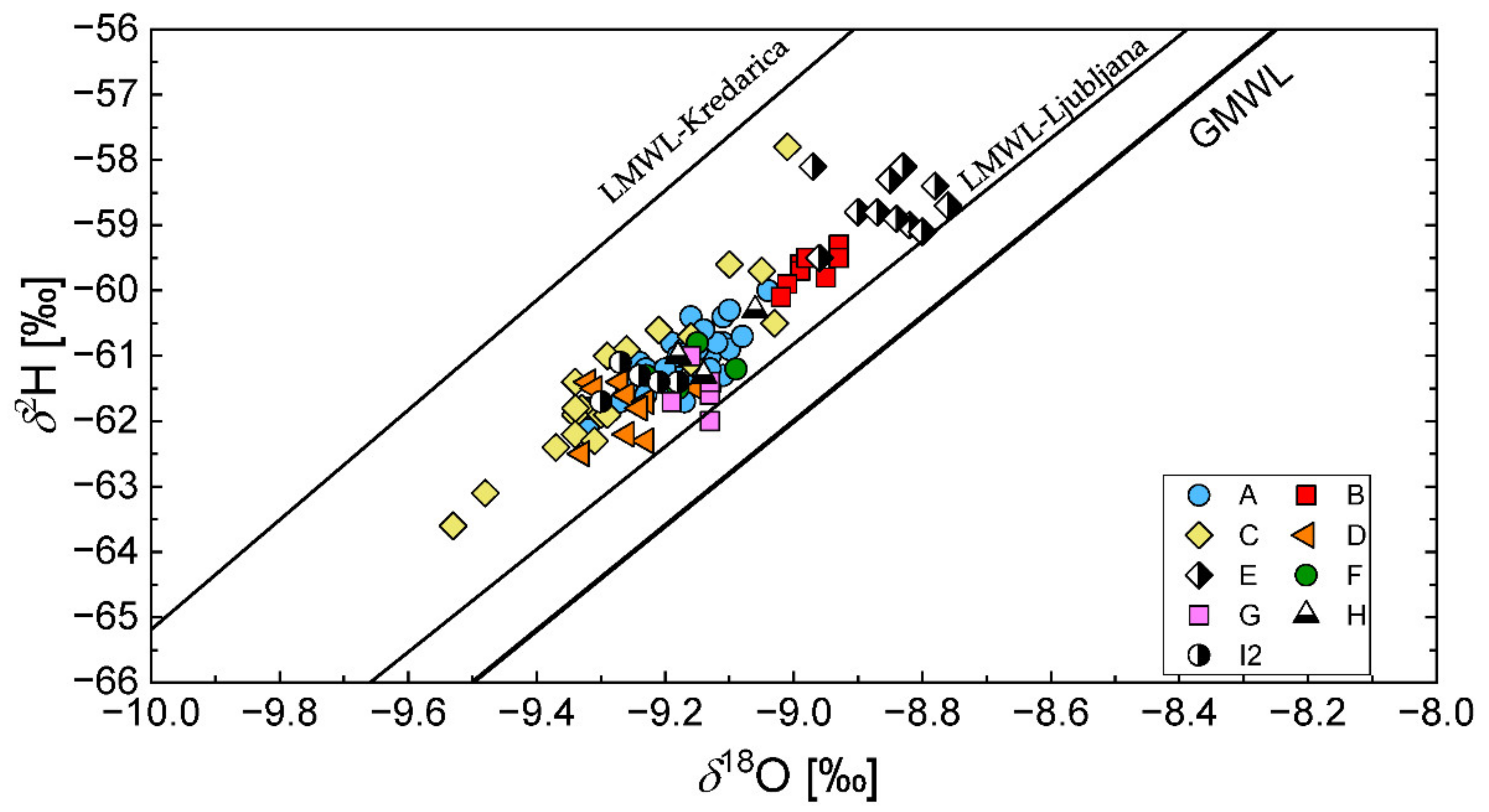
Values of δ2H, δ18O (Figure 2), and d-excess for precipitation ranged between −107.2‰ and −20.0‰, between −14.79‰ and −3.75‰ and between 4.7 to 14.9‰ for the period 2016–2018, respectively. The most positive isotope signature is characteristic for warmer summer months and a more negative signature for colder winter months (Table 1). When comparing seasonal differences during 2018 to the previous three-year averages (Table 1), we observe the highest difference for September–November 2018, i.e., the more positive δ2H and δ18O values, which can be attributed to the higher average air temperature in 2018. The local water meteoric water lines (LMWL) for Ljubljana and Kredarica in the period 2016–2018 were calculated using PWRMA [26,35] and are: δ2H = (7.82 ± 0.16) × δ18O + (9.61 ± 1.37) (r2 = 0.99; N = 35) and δ2H = (8.42 ± 0.19) × δ18O + (18.98 ± 2.09) (r2 = 0.99; N = 34) (Figure 3). The LMWL for the Ljubljana plot is parallel to the GMWL, while the LMWL for Kredarica is plotted above the LMWL for Ljubljana, suggesting different moisture sources in the upper River Sava drainage area than in Ljubljana.
3.3. The Whole Urban Water Supply System
The sample data set of T, EC, pH, TA, δ2H, δ18O, d-excess and δ13CDIC, is presented in [24]. Their median (Me), standard deviation (SD), minimum (min), maximum (max) and ranges are presented in Table 2, while the WSA and TSS averages are presented in [43]. In addition, Table 2 also contains data for CČN and the three sampling locations along the River Sava (Šentjakob, Črnuče and Brod).
The outflow from CČN had the highest values of T, EC, pH, and TA, while the values of δ2H, δ18O and δ13CDIC were lower compared to the median values for the whole system (Table 2). Similarly, T and pH values are higher at the three sampling locations along the River Sava, while EC and TA values are lower than the median values for the whole system. Distinct differences could be observed between more enriched δ2H and δ18O values for the whole system compared to more depleted surface water resulting from different system processes. In addition, other processes (i.e., mixing surface water with precipitation) can cause more positive values observed in other components of the WSS. The average d-excess of the River Sava is 12.3‰ reflecting the contribution of precipitation of the mixed Atlantic−Mediterranean origin [44]. The δ13CDIC values of surface water and wastewater effluent from the CČN treatment plant are more positive than the median values of the whole system. Data for surface water (three locations) and from the CČN were omitted in further evaluation.
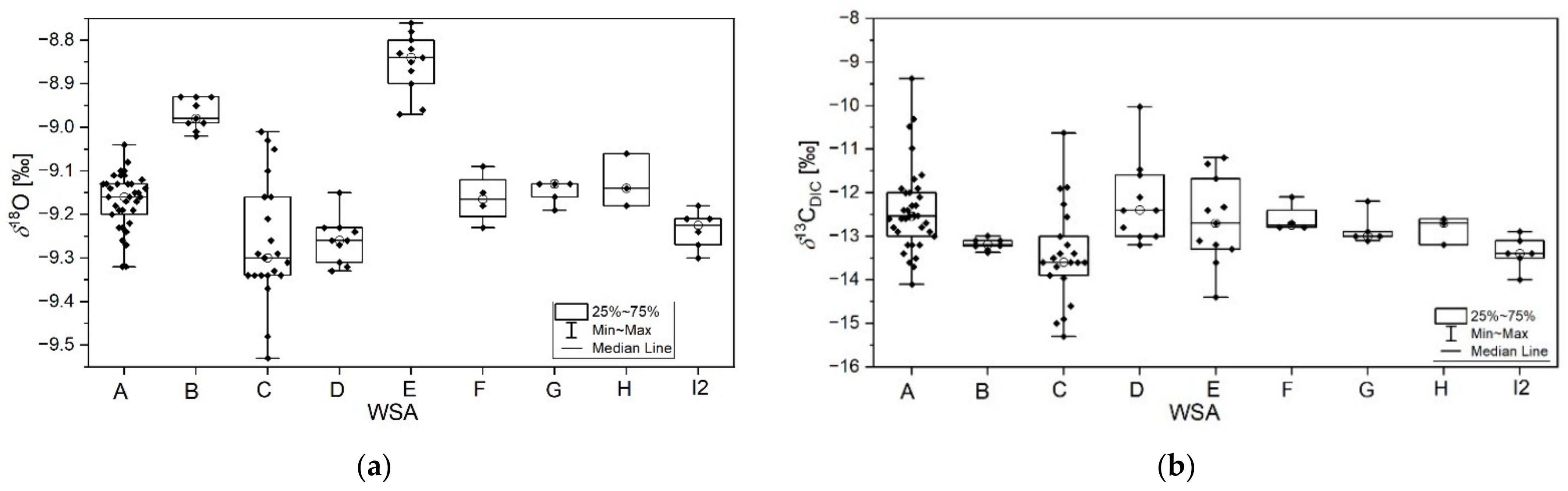
The highest water temperature in the WSS was observed for samples collected in September 2018, corresponding to the highest daily air temperature for that month. The highest EC and pH values were also measured in September 2018, with median values of 508.6 µS/cm and 7.7, respectively. Isotopic signatures were positive during September 2018, with mean values of −60.3‰, −9.10‰, and −12.4‰ for δ2H, δ18O, and δ13CDIC, respectively. In contrast, the most negative isotopic compositions were determined in November 2018 with −61.3‰, −9.21‰, and −13.1‰, respectively. A strong positive correlation (≥0.7; p ≤ 0.001) was observed between EC and TA and δ2H and δ18O, while a strong negative correlation (≥−0.6; p ≤ 0.001) was observed between TA and δ13CDIC (Figure 4a). Associations between sampling months and δ2H and δ18O values were tested. However, differences were only statistically significant for δ2H. A statistically significant correlation was observed between sampling months and δ13CDIC. Total alkalinity ranged from 3.4 mM to 7.4 mM. The highest alkalinity is observed at Brest wellfields, while lower alkalinity is observed at the Hrastje wellfields. In this study, the δ13CDIC values ranged from −15.3‰ (Brest-9) to −9.4‰ (VD-Kleče 7) with a median of −12.9 ± 1‰. The lowest δ13CDIC values were recorded at Brest wellfield, while the highest δ13CDIC was observed at Kleče wellfield (Figure 5b). The total alkalinity (Table 2) is much lower in river water samples (3.3 mM to 3.4 mM) than in groundwater samples (3.4 mM to 7.4 mM). The δ13CDIC values in river water (9.2 to −7.7‰) are higher than in groundwater (–15.3 to −9.4‰) due to the equilibration of CO2 with the atmosphere [45].
Plotting δ2H and δ18O data from all sampling locations in the dual-isotope space (Figure 3) revealed slight differences between different WSA; however, the differences were significant for δ2H and δ18O between some WSA (p ≤ 0.001). The most enriched values were observed for samples from the WSA Šentvid. Samples collected from this WSA are statistically significantly different from other WSA except for Hrastje WSA (Figure 5a). The highest range is observed for samples collected at WSA Brest (0.52‰) with the most negative values of δ18O and δ2H. All samples plot below the LMWL-Kredarica [26], representing the upper part of the River Sava recharge area and above GMWL and LMWL-Ljubljana (Figure 3). However, we observed no statistically significant difference between components and δ2H, δ18O or δ13CDIC, while a statistically significant difference (p ≤ 0.05) was observed between d-excess and different components in the WSS.
3.3.1. Characteristics of the Groundwater from Wells
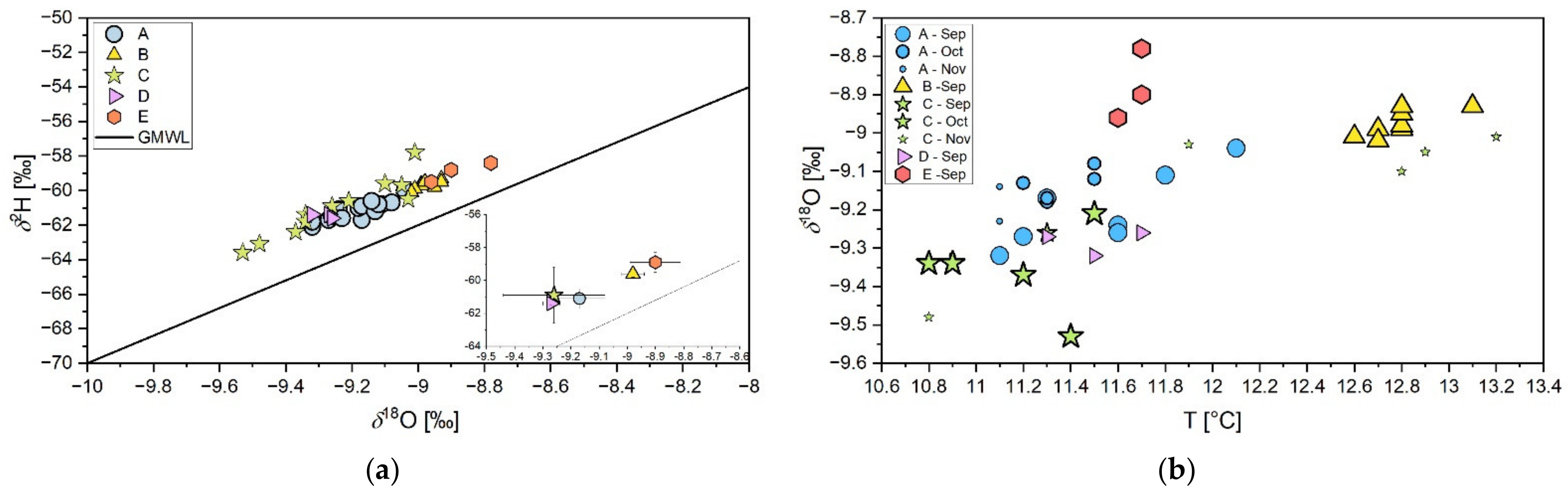
An objective of this research was to sample all 44 active wells in the WSS from both aquifers. However, water samples were only collected from 41 wells. The isotopic composition ranged from −63.6‰ to −57.8‰, from −9.53‰ to −8.75‰ and from 11.7 to 14.3 for δ2H, δ18O and d, respectively. The groundwater is scattered along the LMWL. The same median d-excess of 12‰ was observed for the LP aquifer and the River Sava at all three locations observed in the investigation [14]. Again, the most positive δ18O value can be observed for the Šentvid wellfield (E), followed by the Hrastje wellfield (B) (Figure 6a); moreover, this can also be observed when the median values of wells regarding WSA are plotted (Figure 6a). The most negative values were observed from the deeper wells in Brest: Brest 2a and Brest 4a (S1) [24], which were observed by [17] and attributed to the recharge from higher altitudes.
In the Hrastje, Jarški prod and Šentvid wellfields, more positive isotopes values correlate with distance from the River Sava and EC. Conversely, in the Kleče wellfield, no such trend can be observed where in general, δ18O is decreasing from the outer wells to the central part (Kleče-7) (S1). The outermost well, Kleče-12, presents an exception in this trend with a more negative value. The same trend can be observed for EC values, which decrease with distance from the central part of the wellfield. Again, the Kleče-12 stands out with a more negative δ18O value than the other outer wells. This finding is related to water extraction from the deeper parts of the aquifer (60–100 m). In the northern part of the Kleče wellfield, δ18O and EC values decrease with the distance from the River Sava (S1) [24].
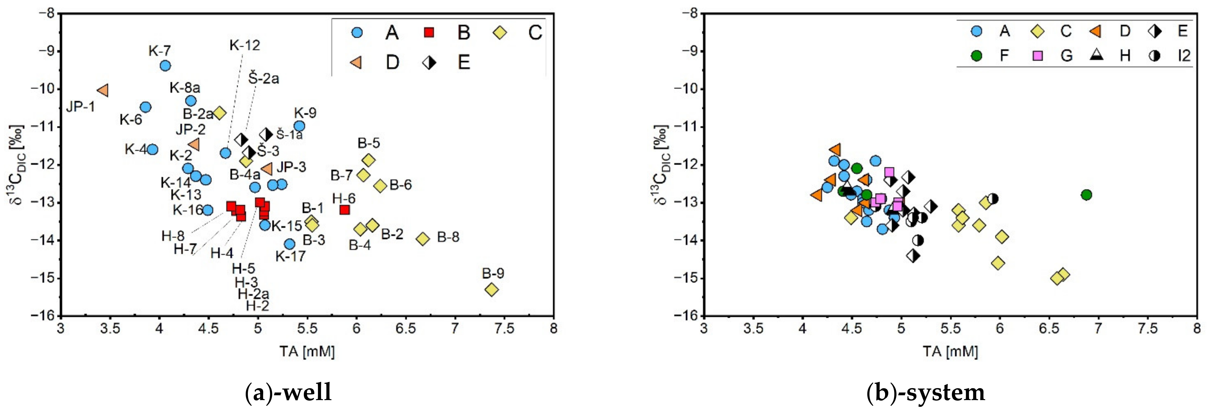
When δ18O is plotted against temperature, the highest temperatures were recorded for those wells sampled in September 2018 from the Hrastje wellfield. In addition, high temperatures were also recorded at Brest-1, Brest-2, and Brest-3 in November 2018 (Figure 6b). The reason can be that these wells are shallower (S1). Also, the δ13CDIC values in groundwater ranged from −15.3‰ to −9.4‰ (Figure 7), specifically, from −14.1‰ to −9.4‰ in the LP and −15.3‰ to −10.6‰ in LB.
The Kleče wellfield is the most important tap water source in the LP and is annually monitored for major cations, anions, organic pollutants, and microbiological parameters. Basic physical and chemical parameters (EC, concentrations of Ca2+, Mg2+, HCO3− and pH) indicate that the fundamental properties of groundwater in the area (S1) depend on the location of the well inside the wellfield [46]. Monitoring results [46] also show that the lowest pH and EC values occur in the central part (Kleče-4); the same low value was also observed in the present study, where δ13CDIC values were −11.6‰ at Kleče-4 (Figure 7a). In the central part of the wellfield, higher δ13CDIC values are likely due to equilibration with river water. At Kleče-3, higher EC levels and δ13CDIC values of −12.6‰ (measured in this study) are due to only a few meters of filter section in the saturated zone [46], indicating a higher soil CO2 contribution. Kleče-12 deviates from other wells and covers aquifers from a depth of 60 to 100 m (S1) with a δ13CDIC value of −11.7‰. Kleče-17 has a similar recharge area as Kleče-11 and 10 and has a similar chemical composition [46]. This observation is also reflected in more negative δ13CDIC values determined in the present study [24]. In the Hrastje well field, the δ13CDIC values of groundwater are, due to longer residence time of the surface water, more homogeneous in comparison to the Kleče wellfield where the δ13CDIC values are more scattered (−13.6 to −9.4‰).
At LB, higher EC and TA (Figure 7a) values were detected in Brest-8 (608.2 µS/cm, 8.33) and Brest-9 (660 µS/cm, 7.22) that capture water from the shallow aquifer. The most positive δ13CDIC (−10.6‰) was observed at Brest-2a (Figure 7a). Brest-4a captures groundwater from depths of 30.3 to 99.3 m (S1) and represents a much broader area than Brest-2a. As a consequence, Brest-4a had lower pH (7.63) and δ13CDIC (−11.9‰) values compared to Brest-2a (7.82 and −10.6‰, respectively). Brest-9 had the most negative δ13CDIC value (−15.3‰), indicating the highest level of soil CO2. Also, long-term monitoring (2011–2019) revealed that Ca2+, Mg2+, and HCO3− were higher in shallower wells than in deeper wells, while the trend was the opposite for pH values. Basic hydro-chemical properties of drinking water in the Holocene aquifer in Brest, especially in shallower wells, are influenced by the Iška River and vary depending on the distance from the river [47]. Therefore, the effect of river water was most apparent in Brest-1 with a δ13CDIC value of −13.5‰ [48]. Unfortunately, the δ13CDIC value in the River Iška was not measured.
The Šentvid wellfield has δ13CDIC values from −11.7 to −11.2‰, while a broader range of values is observed at Jarški prod (−12.1 to −10.0‰). The lowest EC was measured at the Jarški prod WSS. The WSS at Šentvid has higher EC values than the WSS at Kleče since the WSS at Šentvid is positioned outside the main groundwater flow at LP [48]. Higher δ13CDIC values were also observed at Jarški prod-1, 2 and 3 due to their distance from the river water. A higher δ13CDIC value (−10.0‰) was also observed at Jarški prod–1 (closer to the River Sava), while at Jarški prod–3, δ13CDIC values were more negative due mainly to recharge from precipitation being comparable to δ13CDIC values from wells located at the Šentvid wellfield [48].
The δ13CDIC values in the River Sava (Table 2) were more positive (−9.2‰ to −7.7‰) than those in wells in LP and LB, suggesting that δ13CDIC values in groundwater are influenced by water-soil-rock interactions, i.e., degradation of organic matter and carbonate dissolution [49]. At the same time, in river water, equilibration of CO2 occurs [45].
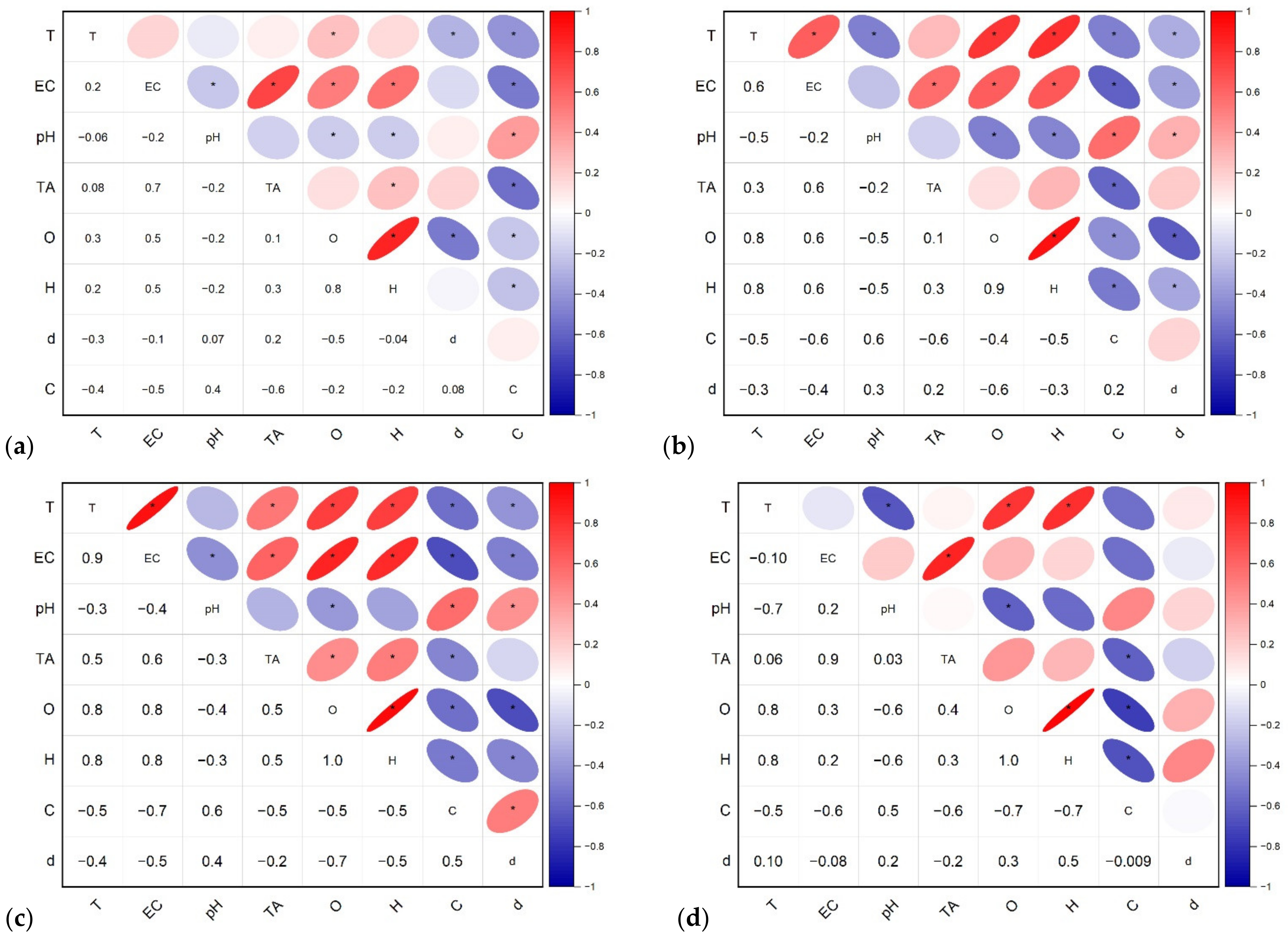
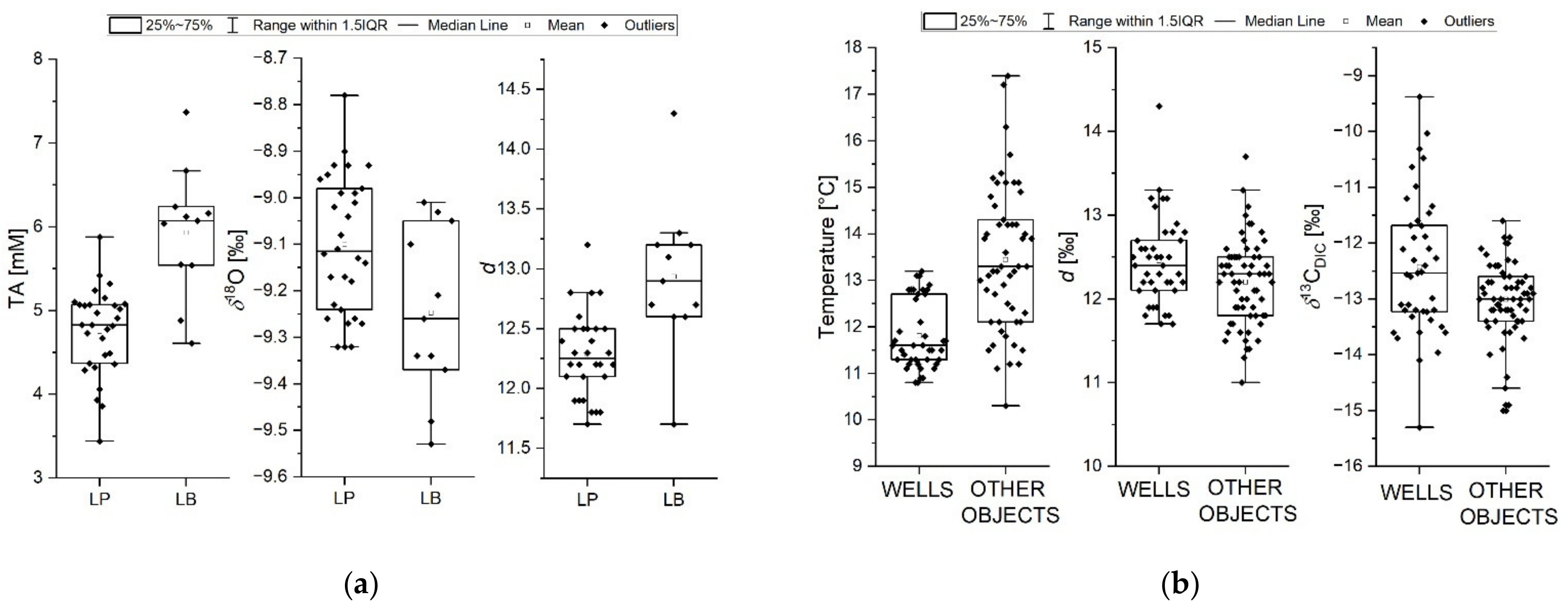
In the present study, a significant (r > 0.6) positive correlation between well parameters was observed between T and EC, δ18O and δ2H, EC and TA, δ18O and δ2H, pH and δ13CDIC and between δ18O and δ2H. Strong (>−0.7) statistically significant negative correlation was observed between δ13CDIC and EC and TA and between δ18O and d, with Spearman’s rank coefficients (rs) (p ≤ 0.005; Figure 4b). When we compare parameters only for LP and LB aquifers (Figure 4c,d), the correlation results change more for LB. The LB aquifer is presented by a strong significant positive correlation between TA and EC and δ18O and δ2H. Also, a strong significant negative correlation is observed between pH and T, δ18O and δ2H, and between δ13CDIC and δ18O and δ2H (Figure 4d). A statistically significant difference is also observed between LP and LB (p ≤ 0.05) regarding TA, δ18O and d-excess (Figure 8a).
Associations were also tested between the wellfields and T, EC, δ18O, δ2H and δ13CDIC. Statistically significant differences were observed for T, EC, TA, δ18O, δ2H, d-excess, and δ13CDIC (p ≤ 0.05), but not between all locations. The highest median T and EC were observed for wells in Hrastje, while the median TA and d were the lowest. The wells in Hrastje, T, pH, TA, and d-excess all showed the smallest range of values. Small ranges in values are also observed for δ18O, δ2H, and δ13CDIC in wells from Hrastje, Jarški prod, and Šentvid. Except for Kleče and Brest, which were collected over three months, all other samples were collected during the same month.
Samples collected in October and November from the wells in Kleče and Brest wells were excluded from the dataset for further evaluation to see if such associations changed. In September 2018, 7, 9, 5, 3, and 3, water samples were collected from wells in Kleče, Hrastje, Brest, Jarški prod, and Šentvid, respectively. In addition to T, EC, TA, δ18O, δ2H, d-excess, and δ13CDIC, there are also significant differences in pH (p ≤ 0.05). Again, a high range of δ18O, δ2H, and δ13CDIC values were observed in Kleče and Brest, suggesting that the well water from each wellfield is compositionally different. In the Brest wellfield, this is likely a consequence of water extraction at different depths [17]. In addition, the well’s position defines the unique properties of the groundwater, which can also be seen using other in-situ parameters (T, EC). Moreover, in the Kleče and Brest wellfields, differences can result from different proportions of the source water in each well [14].
3.3.2. Characteristics of Other Components in the Water Supply System
After the water is pumped from the wells, it is distributed to the end users through the WSS. Other components sampled included joint exits from the water pumping station, reservoirs, water treatment locations, water fountains, and water taps. The observed median temperature was 13.5 °C and is statistically different from the wells (1.7 °C higher; Figure 8b), while the median EC and TA values were lower than the well values, although the differences were insignificant. In addition, δ18O, δ2H, and d-excess values ranged from −9.34‰ to −8.76‰, from −62.5‰ to −58.1‰, and from 11.0 to 13.7, respectively. The observed ranges are smaller than those in the wells, indicating a more homogenous drinking water composition. The median values were more positive for samples collected at LP than LB in all components. Likewise, the differences between LP and LB are also statistically significant. This comparison did not include samples collected at the water treatment locations since they were sampled only at LB. Also, no statistically significant difference in δ18O and δ2H values between other WSS components and wells were observed.
The δ13CDIC values of other components in the system were between −15.0‰ and −11.6‰ (Figure 7b), a range smaller than that observed in the wells. The only statistically significant differences were found between LB and LP, with more negative δ13CDIC values recorded at LB due to the influence of organic matter degradation in Brest-9 and other shallow wells in the Brest well field: Brest-1-8 [9]. The samples collected at LB also have high TA values (Figure 8a). The δ13CDIC from water taps ranged from −14.6 to −11.9‰ (Figure 7b) with an average value of −12.9‰, indicating a more significant contribution from the soil. However, carbonate precipitation within the WSS could have a prominent effect on enrichment with 12C [50]. Water fountains had δ13CDIC from −13.7 to −12.1‰, with more negative δ13CDIC vales observed for Brest and more positive values from Kleče. The δ13CDIC values in the reservoirs ranged from −14.4 to −11.6‰ depending on the water supply well, e.g., the Kleče, Šentvid, and Jarški prod wellfields. Among all wellfields, Brest has the most negative δ13CDIC (Figure 7a).
In addition to T, a statistically significant difference is observed between wells and other components in the WSS for d-excess and δ13CDIC (Figure 8b), while no statistically significant differences for the other parameters were observed. A strong significant positive correlation (≥0.7; p ≤ 0.001) was observed between EC and TA and δ2H and δ18O, while a strong negative correlation (≥−0.6; p ≤ 0.001) was observed between TA and δ13CDIC. A higher temperature range in all components in the system is observed, meaning that the temperature in wells is more stable and not affected by the outside temperature. Moreover, the highest temperature was observed in the Hrastje wellfield but is the most variable in the Brest wellfield [24].
4. Conclusions
This study presents the first stable isotope (H, O, and C) investigation of water in the whole urban WSS in Ljubljana, Slovenia, from source to tap. Sampling was performed mainly by JP VOKA SNAGA d.o.o. staff, JSI team members, and volunteers over three months. The results show changes in meteorological and hydrological conditions that could influence the isotope composition of water collected at different locations across the WSS, from well to tap at the end user. The study is important for consumers and water supply managers.
This investigation combines in-situ (i.e., T and EC), stable isotope (i.e., δ18O, δ2H, and δ13CDIC), and total alkalinity data in order to evaluate whether different components (i.e., water treatment location, reservoirs, water taps, preparation of water, drinking water collector, drinking water fountains) to characterize the urban water cycle. Sampling included a collection of 104 water samples from 103 locations from wells, joint exits from the water pumping station, reservoirs, water treatment locations, drinking water fountains, and taps. Sampling was performed at almost all active wells (41 of 44) included in the WSS for the first time. In addition, sampling was also performed at the Sava River, wastewater treatment plant, and precipitation.
The smallest temperature ranges were observed for wells compared to other components of WSS. This suggests that the system itself is more susceptible to the outside temperature. All other observed parameters show higher variability within the wells than the WSS, which suggests that the water is more unified within the WSS. The δ18O and δ2H signatures of precipitation are seasonal, but no such observation could be determined in the WSS due to the limited three-month sampling period. In addition, very little or no effect of meteorological and hydrological changes can be observed. The results show that the isotope composition at LP depends on the location of the well as the fraction of the precipitation and the River Sava is different. The latter was observed at the Hrastje, Jarški prod, and Šentvid wellfields that show increasing δ18O values with distance from the River Sava.
Higher alkalinity and more negative δ13CDIC were observed at the Brest wellfield. Both parameters (TA and δ13CDIC) are negatively correlated. In all investigated wellfields, both processes: degradation of organic matter and dissolution of carbonates, influence to δ13CDIC value. In addition, precipitation of carbonates within WSS could not be excluded. These phenomena shift the δ13CDIC values in groundwater to values that are more negative. δ13CDIC values are a powerful tool for distinguishing between river/groundwater interactions within a WSS and between shallower and deeper wells, including their distance from river water. The interpretation of δ13CDIC in WSS at LB and LP also depends on other factors such as the depth of filters, pumping rates, and the well’s location.
To understand better the possible changes within the system, sampling from source to tap should be performed simultaneously, with samples being collected for additional parameters. Also, additional observations would be advisable due to possible changes in the River Sava (gaining or losing stream) to the LP and the sensitivity of the LP and LB aquifer to climate changes. This preliminary investigation presents a basic understanding of the differences between different groundwater and the WSS and provides baseline information for future investigations.
Supplementary Materials
The following supporting information can be downloaded at: https://www.mdpi.com/article/10.3390/w14132064/s1. Figure S1: The locations of the active wells at Ljubljansko polje and Ljubljansko barje (Atlas okolja (gov.si) and depth of perforated screens in wells (JP VOKA SNAGA d.o.o.).
Author Contributions
Conceptualization, P.V., T.K., B.B.Ž. and B.J.; formal analysis, K.N.; investigation, P.V., T.K., B.B.Ž. and B.J.; resources, P.V., T.K., B.B.Ž. and B.J.; data curation, K.N., P.V., T.K., B.B.Ž. and B.J.; writing—original draft preparation, K.N.; writing—review and editing, K.N., P.V., T.K., B.B.Ž. and B.J.; visualization, K.N.; supervision, P.V.; funding acquisition, P.V. All authors have read and agreed to the published version of the manuscript.
Funding
This research was funded by Slovenian Research Agency—ARRS Programme (P1-0143), Young research program (PR-09780) and IAEA CRP—Use of Isotope Techniques for the Evaluation of Water Sources for Domestic Supply in Urban Areas (F33024, No. 22843).
Informed Consent Statement
Not applicable.
Data Availability Statement
The data presented in this study are openly available in PANGAEA at https://doi.pangaea.de/10.1594/PANGAEA.914586 [24] (accessed on 27 June 2022).
Acknowledgments
Special thanks are due to S. Žigon for his valuable help with H, O and C isotope analysis, N. Močnik for measurement of total alkalinity, and M. Žitnik for sampling.
Conflicts of Interest
The authors declare no conflict of interest.
References
- Larsen, T.A.; Hoffmann, S.; Lüthi, C.; Truffer, B.; Maurer, M. Emerging Solutions to the Water Challenges of an Urbanizing World. Science 2016, 352, 928–933. [Google Scholar] [CrossRef] [PubMed]
- McGrane, S.J. Impacts of Urbanisation on Hydrological and Water Quality Dynamics, and Urban Water Management: A Review. Hydrol. Sci. J. 2016, 61, 2295–2311. [Google Scholar] [CrossRef]
- Tipple, B.; Jameel, Y.; Chau, T.; Mancuso, C.; Bowen, G.; Dufour, A.; Chesson, L.; Ehleringer, J. Stable Hydrogen and Oxygen Isotopes of Tap Water Reveal Structure of the San Francisco Bay Area’s Water System and Adjustments during a Major Drought. Water Res. 2017, 119, 212–224. [Google Scholar] [CrossRef] [PubMed]
- Jameel, Y.; Brewer, S.; Fiorella, R.P.; Tipple, B.J.; Terry, S.; Bowen, G.J. Isotopic Reconnaissance of Urban Water Supply System Dynamics. Hydrol. Earth Syst. Sci. 2018, 22, 6109–6125. [Google Scholar] [CrossRef] [Green Version]
- Kuhlemann, L.; Tetzlaff, D.; Soulsby, C. Urban Water Systems under Climate Stress: An Isotopic Perspective from Berlin, Germany. Hydrol. Processes 2020, 34, 3758–3776. [Google Scholar] [CrossRef]
- Kendall, C.; Doctor, D.H. Stable Isotope Applications in Hydrologic Studies. Treatise Geochem. 2003, 5, 605. [Google Scholar] [CrossRef]
- Clark, I.; Fritz, P. Environmental Isotopes in Hydrogeology; CRC Press: Boca Raton, FL, USA, 1997; Volume 1997, ISBN 978-0-429-06957-4. [Google Scholar]
- Du, M.; Zhang, M.; Wang, S.; Meng, H.; Che, C.; Guo, R. Stable Isotope Reveals Tap Water Source under Different Water Supply Modes in the Eastern Margin of the Qinghai–Tibet Plateau. Water 2019, 11, 2578. [Google Scholar] [CrossRef] [Green Version]
- Atekwana, E.A.; Krishnamurthy, R.V. Seasonal Variations of Dissolved Inorganic Carbon and δ13C of Surface Waters: Application of a Modified Gas Evolution Technique. J. Hydrol. 1998, 205, 265–278. [Google Scholar] [CrossRef]
- De Wet, R.F.; West, A.G.; Harris, C. Seasonal Variation in Tap Water δ2H and δ18O Isotopes Reveals Two Tap Water Worlds. Sci. Rep. 2020, 10, 13544. [Google Scholar] [CrossRef]
- Sánchez-Murillo, R.; Esquivel-Hernández, G.; Birkel, C.; Ortega, L.; Sánchez-Guerrero, M.; Rojas-Jiménez, L.D.; Vargas-Víquez, J.; Castro-Chacón, L. From Mountains to Cities: A Novel Isotope Hydrological Assessment of a Tropical Water Distribution System. Isot. Environ. Health Stud. 2020, 56, 606–623. [Google Scholar] [CrossRef]
- Leslie, D.; Welch, K.; Lyons, W.B. Domestic Water Supply Dynamics Using Stable Isotopes δ18O, δD, and d-Excess. J. Water Resour. Prot. 2014, 6, 1517–1532. [Google Scholar] [CrossRef] [Green Version]
- Bračič Železnik, B.; Jamnik, B. Javna oskrba s pitno vodo. In Podtalnica Ljubljanskega Polja; Rejec Brancelj, I., Smrekar, A., Kladnik, D., Eds.; Založba ZRC: Ljubljana, Slovenia, 2005; pp. 101–120. (In Slovene) [Google Scholar]
- Vrzel, J.; Solomon, D.K.; Blažeka, Ž.; Ogrinc, N. The Study of the Interactions between Groundwater and Sava River Water in the Ljubljansko Polje Aquifer System (Slovenia). J. Hydrol. 2018, 556, 384–396. [Google Scholar] [CrossRef]
- Vizintin, G.; Souvent, P.; Veselič, M.; Cencur Curk, B. Determination of Urban Groundwater Pollution in Alluvial Aquifer Using Linked Process Models Considering Urban Water Cycle. J. Hydrol. 2009, 377, 261–273. [Google Scholar] [CrossRef]
- Cerar, S.; Urbanc, J. Carbonate Chemistry and Isotope Characteristics of Groundwater of Ljubljansko Polje and Ljubljansko Barje Aquifers in Slovenia. Sci. World J. 2013, 2013, e948394. [Google Scholar] [CrossRef]
- Urbanc, J.; Jamnik, B. Isotopic investigations of the Ljubljansko barje water resources. Geologija 2002, 45, 589–594. [Google Scholar] [CrossRef]
- Ogrinc, N.; Tamše, S.; Zavadlav, S.; Vrzel, J.; Jin, L. Evaluation of Geochemical Processes and Nitrate Pollution Sources at the Ljubljansko Polje Aquifer (Slovenia): A Stable Isotope Perspective. Sci. Total Environ. 2019, 646, 1588–1600. [Google Scholar] [CrossRef]
- Nagode, K.; Kanduč, T.; Lojen, S.; Bračič Železnik, B.; Jamnik, B.; Vreča, P. Synthesis of Past Isotope Hydrology Investigations in the Area of Ljubljana, Slovenia. Geologija 2020, 63, 251–270. [Google Scholar] [CrossRef]
- Nagode, K.; Kanduč, T.; Zuliani, T.; Bračič Železnik, B.; Jamnik, B.; Vreča, P. Daily Fluctuations in the Isotope and Elemental Composition of Tap Water in Ljubljana, Slovenia. Water 2021, 13, 1451. [Google Scholar] [CrossRef]
- Rejec Brancelj, I.; Smrekar, A.; Kladnik, D. Podtalnica Ljubljanskega Polja; ZRC SAZU, Založba ZRC: Ljubljana, Slovenia, 2004; Volume 10, ISBN 978-961-254-508-6. (In Slovene) [Google Scholar]
- Mencej, Z. The Gravel Fill beneath the Lacustrine Sediments of the Ljubljansko Barje. Geologija 1988, 31, 517–553. [Google Scholar]
- Jamnik, B.; Žitnik, M. Letno Poročilo o Skladnosti Pitne Vode na Oskrbovalnih Območjih v Upravljanju Javnega Podjetja Vodovod Kanalizacija Snaga d. o. o. v Letu 2019; Javno Podjetje Vodovod-Kanalizacija d.o.o.: Ljubljana, Slovenia, 2020; p. 27. [Google Scholar]
- Vreča, P.; Nagode, K.; Kanduč, T.; Lojen, S.; Šlejkovec, Z.; Žigon, S.; Močnik, N.; Bračič Železnik, B.; Jamnik, B.; Žitnik, M. Multi-Isotope Characterization of Water Resources for Domestic Supply in Ljubljana, Slovenia. Pangaea 2020. [Google Scholar] [CrossRef]
- Meteo.Si—Uradna Vremenska Napoved Za Slovenijo—Državna Meteorološka Služba RS—Vreme Podrobneje. Available online: https://meteo.arso.gov.si/met/sl/app/webmet/#webmet=vUHcs9WYkN3LtVGdl92LhBHcvcXZi1WZ09Cc1p2cvAncvd2LyVWYs12L3VWY0hWZy9SaulGdugXbsx3cs9mdl5WahxHf (accessed on 5 April 2022).
- Jožef Stefan Institute SLONIP: Slovenian Network of Isotopes in Precipitation. Available online: https://slonip.ijs.si (accessed on 15 April 2022).
- Kern, Z.; Hatvani, I.G.; Czuppon, G.; Fórizs, I.; Erdélyi, D.; Kanduč, T.; Palcsu, L.; Vreča, P. Isotopic ‘Altitude’ and ‘Continental’ Effects in Modern Precipitation across the Adriatic–Pannonian Region. Water 2020, 12, 1797. [Google Scholar] [CrossRef]
- Vreča, P.; Malenšek, N. Slovenian Network of Isotopes in Precipitation (SLONIP)—A Review of Activities in the Period 1981–2015. Geologija 2016, 59, 67–84. [Google Scholar] [CrossRef]
- Gieskes, J.M. The Alkalinity-Total Carbon Dioxide System in Seawater. Mar. Chem. 1974, 5, 123–151. [Google Scholar]
- Dansgaard, W. Stable Isotopes in Precipitation. Tellus 1964, 16, 436–468. [Google Scholar] [CrossRef]
- Spötl, C. A Robust and Fast Method of Sampling and Analysis of δ13C of Dissolved Inorganic Carbon in Ground Waters. Isot. Environ. Health Stud. 2005, 41, 217–221. [Google Scholar] [CrossRef]
- Kanduč, T.; Mori, N.; Kocman, D.; Stibilj, V.; Grassa, F. Hydrogeochemistry of Alpine Springs from North Slovenia: Insights from Stable Isotopes. Chem. Geol. 2012, 300–301, 40–54. [Google Scholar] [CrossRef]
- Craig, H. Isotopic Variations in Meteoric Waters. Science 1961, 133, 1702–1703. [Google Scholar] [CrossRef]
- Crawford, J.; Hughes, C.E.; Lykoudis, S. Alternative Least Squares Methods for Determining the Meteoric Water Line, Demonstrated Using GNIP Data. J. Hydrol. 2014, 519, 2331–2340. [Google Scholar] [CrossRef]
- Pavšek, A.; Vreča, P. Isotopes in Precipitation—Statistics. Available online: https://github.com/nyuhanc/Isotopes-in-precipitation-statistics (accessed on 7 May 2022).
- Kozjek, K.; Dolinar, M.; Skok, G. Objective Climate Classification of Slovenia. Int. J. Climatol. 2017, 37, 848–860. [Google Scholar] [CrossRef]
- Meteo.Si—Uradna Vremenska Napoved Za Slovenijo—Državna Meteorološka Služba RS—Ljubljana. Available online: http://www.meteo.si/met/sl/climate/diagrams/ljubljana/ (accessed on 5 April 2022).
- Cegnar, T. Podnebne razmere v Sloveniji leta 2018. Ujma 2019, 33, 24–39. (In Slovene) [Google Scholar]
- Agencija Republike Slovenije za Okolje. Naše Okolje, Mesečni Bilten Agencije RS za Okolje—September 2018; ARSO: Ljubljana, Slovenia, 2018; p. 102. (In Slovene)
- Agencija Republike Slovenije za Okolje. Naše Okolje, Mesečni Bilten Agencije RS za Okolje—Oktober 2018; ARSO: Ljubljana, Slovenia, 2018; p. 90. (In Slovene)
- Agencija Republike Slovenije za Okolje. Naše Okolje, Mesečni Bilten Agencije RS za Okolje—November 2018; ARSO: Ljubljana, Slovenia, 2018; p. 102. (In Slovene)
- Arhivski Podatki. Available online: http://vode.arso.gov.si/hidarhiv/pov_arhiv_tab.php (accessed on 5 April 2022).
- Vreča, P.; Kanduč, T.; Šlejkovec, Z.; Žigon, S.; Nagode, K.; Močnik, N.; Bračič-Železnik, B.; Jamnik, B.; Žitnik, M. Karakterizacija vodnih virov za javno oskrbo s pitno vodo v Ljubljani s pomočjo različnih geokemičnih analiz. Raziskave S Področja Geod. Geofiz. 2018, 2019, 111–119. (In Slovene) [Google Scholar]
- Ogrinc, N.; Kanduč, T.; Stichler, W.; Vreča, P. Spatial and Seasonal Variations in δ18O and δD Values in the River Sava in Slovenia. J. Hydrol. 2008, 359, 303–312. [Google Scholar] [CrossRef]
- Kanduč, T.; Szramek, K.; Ogrinc, N.; Walter, L.M. Origin and Cycling of Riverine Inorganic Carbon in the Sava River Watershed (Slovenia) Inferred from Major Solutes and Stable Carbon Isotopes. Biogeochemistry 2007, 86, 137–154. [Google Scholar] [CrossRef]
- Jamnik, B.; Žitnik, M. Poročilo o Ugotovitvah Nadzora Podzemne in Pitne Vode v Vodarni Kleče v Obdobju 2011–2020; JP VOKA SNAGA: Ljubljana, Slovenia, 2021. (In Slovene) [Google Scholar]
- Jamnik, B.; Žitnik, M.; Auersperger, P.; Bračič Železnik, B.; Nataša, Č.; Kalšek, I.; Kozjek, M.; Lah, K.; Vrbec, A.; Prestor, J. Poročilo o Ugotovitvah Nadzora Podzemne in Pitne Vode v Vodarni Brest v Obdobju 2011–2019; JP VOKA SNAGA: Ljubljana, Slovenia, 2020; p. 39. (In Slovene) [Google Scholar]
- Jamnik, B.; Auersperger, P. Interne Priloge k Letnemu Poročilu o Skladnosti Pitne Vode na Oskrbovalnih Območjih v Upravljanju Javnega Podjetja Vodovod Kanalizacija Snaga v Letu 2020; JP VOKA SNAGA: Ljubljana, Slovenia, 2021; p. 48. (In Slovene) [Google Scholar]
- Barth, J.A.C.; Cronin, A.A.; Dunlop, J.; Kalin, R.M. Influence of Carbonates on the Riverine Carbon Cycle in an Anthropogenically Dominated Catchment Basin: Evidence from Major Elements and Stable Carbon Isotopes in the Lagan River (N. Ireland). Chem. Geol. 2003, 200, 203–216. [Google Scholar] [CrossRef]
- Aucour, A.-M.; Sheppard, S.M.F.; Guyomar, O.; Wattelet, J. Use of 13C to Trace Origin and Cycling of Inorganic Carbon in the Rhône River System. Chem. Geol. 1999, 159, 87–105. [Google Scholar] [CrossRef]
Figure 1.
Sampling locations for the different water supply areas (WSA) and type of sampling site (TSS). Zoom locations represent the distribution of wells in the respective wellfields. VD = well, ZV = joint exit from the water pumping station, VH = reservoir, PV = water treatment location, PIT = drinking water fountain, PJ = tap in a public building, PP = tap in a private building, CČN = water treatment plant, R = river; A = Kleče, C = Brest, D = Jarški prod, E = Šentvid, F = Hrastje/Jarški prod, G = Kleče/Brest, H = Kleče/Hrastje/Jarški prod, I2 = Kleče/Hrastje/Brest.

Figure 2.
Monthly precipitation totals (mm), average monthly air temperature (°C), water flow (m3/s), water temperature (°C) and δ2H, δ18O in precipitation during 2016–2018. The sampling period September–November 2018 is marked with black lines.
Figure 2.
Monthly precipitation totals (mm), average monthly air temperature (°C), water flow (m3/s), water temperature (°C) and δ2H, δ18O in precipitation during 2016–2018. The sampling period September–November 2018 is marked with black lines.

Figure 3.
Dual isotope plot of the whole water supply system samples compared to the global meteoric water line (GMWL) and local meteoric water line (LMWL) from Ljubljana (2016–2018) and Kredarica (2016–2018). A = Kleče, B = Hrastje, C = Brest, D = Jarški prod, E = Šentvid, F = Hrastje/Jarški prod, G = Kleče/Brest, H = Kleče/Hrastje/Jarški prod and I2 = Kleče/Hrastje/Brest.

Figure 4.
Spearman correlation matrix between determined parameters and (a) the whole urban water supply system (N = 104); wells at (b) Ljubljansko barje and Ljubljansko polje (N = 41); (c) Ljubljansko polje (N = 30); (d) Ljubljansko barje (N = 11). * p ≤ 0.05. H, O and C represent δ2H, δ18O and δ13CDIC, respectively.

Figure 5.
Distribution of (a) δ18O and (b) δ13CDIC regarding different WSA for the whole system (N = 97). For the explanation of the abbreviations, see Section 2.2.
Figure 5.
Distribution of (a) δ18O and (b) δ13CDIC regarding different WSA for the whole system (N = 97). For the explanation of the abbreviations, see Section 2.2.

Figure 6.
(a) Dual isotope plot of wells compared to GMWL. The small picture presents medians of wells regarding the respective wellfield. (b) δ18O vs. T for wells from different wellfields. Different sized symbols represent different sampling months. A = Kleče, B = Hrastje, C = Brest, D = Jarški prod and E = Šentvid.

Figure 7.
Relation between δ13CDIC and TA for samples collected from wells (N = 41) (a) other components of the WSS system (N = 63) (b). A = Kleče, B = Hrastje, C = Brest, D = Jarški prod, E = Šentvid, F = Hrastje/Jarški prod, G = Kleče/Brest, H = Kleče/Hrastje/Jarški prod and I2 = Kleče/Hrastje/Brest.

Figure 8.
(a) Observed statistically significant differences for TA, δ18O, and d-excess between wells presented at Ljubljansko polje (LP; N = 30) and Ljubljansko barje (LB; N = 11). (b) Observed statistically significant differences in T, d-excess, and δ13CDIC between wells (N = 41) and other components in the WSS (N = 63).


Table 1.
Mean precipitation (mm), mean air temperature (°C), and mean isotope composition of precipitation for the three-month periods during 2016–18 and 2018, respectively.
Table 1.
Mean precipitation (mm), mean air temperature (°C), and mean isotope composition of precipitation for the three-month periods during 2016–18 and 2018, respectively.
| Year | Parameters | December–February | March–May | June–August | September–November |
|---|---|---|---|---|---|
| 2016–2018 | P [mm] | 98.2 | 104.8 | 119.8 | 146.7 |
| T [°C] | 1.8 | 12.5 | 22.0 | 11.9 | |
| δ18O [‰] | −10.91 | −7.93 | −5.60 | −8.27 | |
| δ2H [‰] | −76.5 | −53.8 | −35.6 | −53.0 | |
| 2018 | P [mm] | 72.5 | 118.6 | 148.0 | 119.8 |
| T [°C] | 2.3 | 12.6 | 22.0 | 13.0 | |
| δ18O [‰] | −10.88 | −7.18 | −5.95 | −7.20 | |
| δ2H [‰] | −76.2 | −47.8 | −38.7 | −44.3 |
Table 2.
Basic statistic parameters for temperature (°C), electrical conductivity (µS/cm), pH, total alkalinity (mM), and isotope composition of oxygen (δ18O) and hydrogen (δ2H), d-excess and isotopic composition of carbon in dissolved inorganic carbon (δ13CDIC) for all components in the system and the actual values for CČN and locations at the River Sava.
| T (°C) | EC (µS/cm) | pH | TA (mM) | δ2H (‰) | δ18O (‰) | d (‰) | δ13CDIC (‰) | |
|---|---|---|---|---|---|---|---|---|
| Median | 12.7 | 508.55 | 7.7 | 4.9 | −61.2 | −9.16 | 12.3 | −12.9 |
| Standard deviation | 1.5 | 58.1 | 0.2 | 0.7 | 1.1 | 0.15 | 0.5 | 1.0 |
| Minimum | 10.3 | 365.2 | 7.2 | 3.4 | −63.6 | −9.53 | 11.0 | −15.3 |
| Maximum | 17.4 | 660 | 8.4 | 7.4 | −57.8 | −8.76 | 14.3 | −9.4 |
| Range | 7.1 | 294.8 | 1.2 | 4.0 | 5.8 | 0.77 | 3.3 | 5.9 |
| Sava 1–Šentjakob | 15.0 | 345 | 8.17 | 3.3 | −63.0 | −9.40 | 12.2 | −8.0 |
| Sava 2–Črnuče | 15.1 | 345 | 8.23 | 3.4 | −62.4 | −9.39 | 12.7 | −9.2 |
| Sava 3–Brod | 15.1 | 343 | 8.24 | 3.3 | −63.3 | −9.45 | 12.3 | −7.7 |
| CČN | 21.7 | 1086 | 9.9 | 5.9 | −58.2 | −8.68 | 11.2 | −11.9 |
Publisher’s Note: MDPI stays neutral with regard to jurisdictional claims in published maps and institutional affiliations. |
© 2022 by the authors. Licensee MDPI, Basel, Switzerland. This article is an open access article distributed under the terms and conditions of the Creative Commons Attribution (CC BY) license (https://creativecommons.org/licenses/by/4.0/).
Share and Cite
MDPI and ACS Style
Nagode, K.; Kanduč, T.; Bračič Železnik, B.; Jamnik, B.; Vreča, P. Multi-Isotope Characterization of Water in the Water Supply System of the City of Ljubljana, Slovenia. Water 2022, 14, 2064. https://doi.org/10.3390/w14132064
AMA Style
Nagode K, Kanduč T, Bračič Železnik B, Jamnik B, Vreča P. Multi-Isotope Characterization of Water in the Water Supply System of the City of Ljubljana, Slovenia. Water. 2022; 14(13):2064. https://doi.org/10.3390/w14132064
Chicago/Turabian StyleNagode, Klara, Tjaša Kanduč, Branka Bračič Železnik, Brigita Jamnik, and Polona Vreča. 2022. "Multi-Isotope Characterization of Water in the Water Supply System of the City of Ljubljana, Slovenia" Water 14, no. 13: 2064. https://doi.org/10.3390/w14132064
Note that from the first issue of 2016, this journal uses article numbers instead of page numbers. See further details here.