A New Turbulence Model for Breaking Wave Simulations

Abstract

In this paper, the hydrodynamic and free surface elevation fields in breaking waves are simulated by solving the integral and contravariant forms of the three-dimensional Navier–Stokes equations that are expressed in a generalized time-dependent curvilinear coordinate system, in which the vertical coordinate moves by following the free surface. A new $k-l$ turbulence model in contravariant form is proposed; in this model, the mixing length, $l$, is defined as a function of the maximum water surface elevation variation. A new original numerical scheme is proposed. The main element of originality of the numerical scheme consists of the proposal of a new fifth-order reconstruction technique for the point values of the conserved variables on the cell face. This technique, named in the paper as WTENO, allows the choice procedure of the reconstruction polynomials for the point values to be modified in a dynamic way.

1. Introduction

Experimental simulations [1,2,3] and numerical simulations [4,5,6,7,8,9,10,11,12] of hydrodynamic fields, turbulent phenomena and concentration of suspended sediment under breaking waves allow for the analysis of the effects produced by wave motion and coastal structures on the bottom and coastline modifications. In numerical simulations, the definition of the turbulent closure relations under breaking waves is one of the most important issues to adequately represent the three-dimensional velocity fields and the turbulent phenomena that develop near the bottom boundary. It is necessary to simulate the turbulent phenomena in the boundary layer both in the zone that is dominated by turbulent stresses (turbulent core), and in the zone nearest to the bottom (buffer layer).

In the context of three-dimensional simulations of breaking waves [9,10,11], in the literature, the turbulent phenomena are represented by many authors using the Smagorinsky turbulence model. In this model, the turbulent stress tensor is related to the strain rate tensor through the Smagorinsky coefficient. The numerical simulations that use this turbulence model are significantly influenced by this coefficient. It has been demonstrated by Ma [9] that the above-mentioned turbulence model (even though collocated in the context of shock-capturing numerical schemes) is not able to correctly evaluate the dissipation of the energy of the averaged motion. When in the Smagorinsky model, high values of the above-mentioned coefficient are used; this model overestimates the turbulent phenomena (in the shoaling zone, in the region around the breaking point and in the surf zone without distinction) and produces a significant reduction in the wave height. The existing Smagorinsky models underestimate the turbulent phenomena, thus the task of dissipating the energy of the averaged motion in the surf zone is given to the numerical scheme.

In the context of three-dimensional simulations of breaking waves, in order to reduce the spurious oscillations that are generated in the proximity of the shock, many authors [9,10,11,12] use low-order shock-capturing numerical schemes that adopt TVD (Total Variation Diminishing) reconstruction techniques and approximate Riemann solvers. In [9,10,11] the Poisson equation is written in terms of primitive variables (with $u^l$ as the flow velocity components, and H as the water depth). According to [13], the use of the primitive variable can produce incorrect velocity propagation of the shocks. In order to reduce spurious oscillations in the proximity of the shocks and their propagations, the low-order numerical scheme dissipates the largest part of the kinetic energy of the averaged motion. Furthermore, the approximate Riemann solver does not consider the solution for the rarefaction waves; this incomplete solution produces an excess of numerical dissipation of kinetic energy of the averaged motion. These numerical schemes introduce too much energy dissipation of the averaged motion in the numerical simulations, causing an underestimation of the wave height in the shoaling zone, and an incorrect location of the breaking point.

Many authors use a turbulence model in which the eddy viscosity is a function of the turbulent kinetic energy, $k$, and the mixing length, $l$ [4,12]. In the existing $k-l$ turbulence models, the production and dissipation of turbulent kinetic energy are represented in the same way, both before and after the breaking point. In other words, in these models the existing significant difference between the phenomena of production and dissipation of turbulent kinetic energy in the different above-mentioned zones (shoaling zone, region around the breaking point and surf zone) are not taken into account.

In the simulation of wave breaking, both in the Smagorinsky model and in the $k-l$ model present in the literature, the discretization of the calculation domain does not involve the bottom boundary layer. The above-mentioned models place the first calculation grid cell outside the boundary layer; hence, they do not adequately calculate the production of turbulent kinetic energy in the buffer layer nor in the turbulent core of the boundary layer at the bottom. Consequently, the bottom turbulent phenomena are not represented in these models.

In order to reduce the average motion energy dissipation introduced in the numerical schemes and thus leave the task of dissipating that energy only to the turbulence model, this paper proposes a new shock-capturing numerical scheme based on three elements of novelty in addition to a new $k-l$ turbulence model. The proposed numerical scheme solves the three-dimensional Navier–Stokes in integral contravariant form expressed in a generalized time-dependent curvilinear coordinate system, in which the vertical coordinate moves by following the free surface. The first element of novelty of this numerical scheme is that the equations of motion and the Poisson equation (that is the Laplacian of the scalar potential) are expressed in terms of the conserved variables ($H{u}^l$, and $H$). The second element of novelty is related to the reconstruction technique for the point values of the conserved variables on the cell face. The numerical scheme is based on a new fifth-order reconstruction technique named in this paper as WTENO (Wave-Targeted Essentially Non-Oscillatory). This reconstruction technique uses different polynomials defined on contiguous cells, and also uses a so-called cut-off function (which varies in space and time) that depends on the polynomial regularity, and on the definition of a dynamic threshold (which also varies in space and time), which varies as a function of the steepness of the wave fronts. This reconstruction technique ensures high-order accuracy, good non-oscillatory properties and avoids excessive dissipation of the energy of the averaged motion due to the TVD reconstruction technique. The last element of novelty is the use of an exact solution of the Riemann problem for the time advancing of the point values of the conserved variables on the cell faces. By using the new high-order numerical scheme, it is possible to leave the task of dissipating the energy of the averaged motion to the turbulence model.

A new $k-l$ turbulence model is proposed that overcomes the limitations introduced by the Smagorinsky and existing $k-l$ models. In the new turbulence model, the mixing length is defined as a function of the maximum water surface elevation spatial variation and its second derivative; in this way, the existing significant differences between the turbulent phenomena, that occur before and after the breaking point, are taken into account.

2. Governing Equations

A new model is proposed for the simulation of hydrodynamic and free-surface elevation fields under breaking waves, based on the solution of the three-dimensional Navier–Stokes equations. Let $H$ be the total water depth, and $u^l \left(l=1,3\right)$ be the contravariant components of the velocity. The three-dimensional Navier–Stokes equations are expressed in integral contravariant form, without the Christoffel symbols, in terms of the conserved variables $H$ and $H{u}^l$.

Let us assume a reference system in which $x^1$ and $x^2$ are the Cartesian horizontal coordinates, and $x^3$ is the Cartesian vertical coordinate pointing upward with the origin on the undisturbed water surface. In this reference system, the total water depth is given by $H\left(x^1,x^2,t\right)=h\left(x^1,x^2\right)+\eta \left(x^1,x^2,t\right)$, where $h$ is the undisturbed water depth and $\eta$ is the free-surface elevation with respect to the undisturbed water level. By defining the curvilinear coordinates, $\left({\xi }^1, {\xi }^2, {\xi }^3, \tau \right)$, the specific coordinate transformation from the Cartesian coordinate system, $\left(x^1,x^2,x^3,t\right)$, to the curvilinear one, is given by the following:

$${\xi }^1={\xi }^1\left(x^1,x^2,x^3\right);\hspace{1em}{\xi }^2={\xi }^2\left(x^1,x^2,x^3\right);\hspace{1em}{\xi }^3=\frac{x^3+h\left(x^1,x^2\right)}{H\left(x^1,x^2,t\right)};\tau =t$$

(1)

The coordinates ${\xi }^1$ and ${\xi }^2$ are not time dependent, whereas the vertical coordinate ${\xi }^3$ moves with the free surface according to the $\sigma$-coordinate transformation by [14] which we adapt to the proposed reference system. ${\overrightarrow{g}}_{\left(l\right)}=\partial \overrightarrow{x}/\partial {\xi }^l$ indicates the covariant base vectors, and ${\overrightarrow{g}}^{\left(l\right)}=\partial {\xi }^l/\partial \overrightarrow{x}$ indicates the contravariant base vectors. The metric tensor and its inverse are defined by $g_{lm}={\overrightarrow{g}}_{\left(l\right)}·{\overrightarrow{g}}_{\left(m\right)}$ and $g^{lm}={\overrightarrow{g}}^{\left(l\right)}·{\overrightarrow{g}}^{\left(m\right)}$ ($l,m=1,3$), where the symbol “$·$” indicates the vector scalar product. The Jacobian of the transformation is given by $\sqrt{g}=H\sqrt{g_0}$, in which $\sqrt{g_0}=\overrightarrow{k}·\left({\overrightarrow{g}}_{\left(1\right)}\mathsf{\Lambda }{\overrightarrow{g}}_{\left(2\right)}\right)$; $\overrightarrow{k}$ indicates the vertical unit vector and $\mathsf{\Lambda }$ indicates the vector product.

The momentum balance equation expressed in integral contravariant form in a time-dependent curvilinear coordinate system is given by the following:

$$\begin{gathered} \frac{\partial \overline{H{u}^r}}{\partial \tau }= \\ -\frac{\mathsf{\Delta }t}{\mathsf{\Delta }{V}_0\sqrt{g_0}}{\displaystyle \sum }_{\alpha =1}^3\{{{\displaystyle \int }}_{\mathsf{\Delta }{A}_o^{\alpha +}}\left[{\overrightarrow{\tilde{g}}}^{\left(r\right)}·{\overrightarrow{g}}_{\left(k\right)}\left(H{u}^k\right)\left(\left(H{u}^{\alpha }/H\right) -v^{\alpha }\right)+{\overrightarrow{\tilde{g}}}^{\left(r\right)}·{\overrightarrow{g}}^{\left(\alpha \right)}G\left(\eta H\right) \right]\sqrt{g_0}d{\xi }^{\beta }d{\xi }^{\gamma }- \\ {{\displaystyle \int }}_{\mathsf{\Delta }{A}_o^{\alpha -}}\left[{\overrightarrow{\tilde{g}}}^{\left(r\right)}·{\overrightarrow{g}}_{\left(k\right)}\left(H{u}^k\right)\left(\left(H{u}^{\alpha }/H\right) -v^{\alpha }\right)+{\overrightarrow{\tilde{g}}}^{\left(r\right)}·{\overrightarrow{g}}^{\left(\alpha \right)}G\left(\eta H\right)\right]\sqrt{g_0}d{\xi }^{\beta }d{\xi }^{\gamma }\}+ \\ \frac{\mathsf{\Delta }t}{\mathsf{\Delta }{V}_0\sqrt{g_0}}{\displaystyle \sum }_{\alpha =1}^3\{{{\displaystyle \int }}_{\mathsf{\Delta }{A}_o^{\alpha +}}{\overrightarrow{\tilde{g}}}^{\left(r\right)}·{\overrightarrow{g}}_{\left(k\right)}\frac{T^{k\alpha }}{\rho }H\sqrt{g_0}d{\xi }^{\beta }d{\xi }^{\gamma }-{{\displaystyle \int }}_{\mathsf{\Delta }{A}_o^{\alpha -}}{\overrightarrow{\tilde{g}}}^{\left(r\right)}·{\overrightarrow{g}}_{\left(k\right)}\frac{T^{k\alpha }}{\rho }H\sqrt{g_0}d{\xi }^{\beta }d{\xi }^{\gamma }\} \end{gathered}$$

(2)

where $\overline{H{u}^l}$ is the cell average value of the conserved variable $H{u}^l$, $u^k \left(k=1,3\right)$ are the contravariant components of the fluid velocity, $v^{\alpha } \left(\alpha =1,3\right)$ are the contravariant components of the velocity of the moving coordinates; ${\overrightarrow{\tilde{g}}}^{\left(l\right)}$ is the covariant base vector defined at the center of the control volume. $V_0=\mathsf{\Delta }{\xi }^1\mathsf{\Delta }{\xi }^2\mathsf{\Delta }{\xi }^3$; $\mathsf{\Delta }{A}_0^{\alpha }=\mathsf{\Delta }{\xi }^{\beta }\mathsf{\Delta }{\xi }^{\gamma };$ $\mathsf{\Delta }{A}_0^{\alpha +}$ and $\mathsf{\Delta }{A}_0^{\alpha -}$ are the boundary surfaces of the control volume $\mathsf{\Delta }{V}_0$ on which the coordinate ${\xi }^{\alpha }$ is constant, that surfaces are located in correspondence to the larger and smaller values of ${\xi }^{\alpha }$ ($\alpha$, $\beta$ and $\gamma$ are cyclic). $T^{k\alpha }$ are the contravariant components of the stress tensor that contain the dynamic pressure term; $\rho$ is the fluid density and $G$ is the gravitational acceleration.

The equation relative to the movement of the free surface expressed in integral contravariant form in a time-dependent curvilinear coordinate system is given by the following equation:

$$\frac{\partial \overline{H}}{\partial \tau }=\frac{1}{\mathsf{\Delta }{A}_o^3\sqrt{g_0}}{\displaystyle \sum }_{\alpha =1}^2\left[{{\displaystyle \int }}_0^1{{\displaystyle \int }}_{\mathsf{\Delta }{\xi }_o^{\alpha +}}H{u}^{\alpha }\sqrt{g_0}d{\xi }^{\beta }d{\xi }^3-{{\displaystyle \int }}_0^1{{\displaystyle \int }}_{\mathsf{\Delta }{\xi }_o^{\alpha -}}H{u}^{\alpha }\sqrt{g_0}d{\xi }^{\beta }d{\xi }^3\right]$$

(3)

where $\overline{H}$ is the cell average value of the variable $H$, and $\mathsf{\Delta }{\xi }_o^{\alpha +}$ and $\mathsf{\Delta }{\xi }_o^{\alpha -}$ (with $\alpha =1,2)$ are the contour lines of the surface element $\mathsf{\Delta }{A}_o^3=\mathsf{\Delta }{\xi }^1\mathsf{\Delta }{\xi }^2$ on which ${\xi }^{\alpha }$ is constant and are located, respectively, in correspondence to the larger and smaller values of ${\xi }^{\alpha }$.

The numerical scheme that is adopted to advance in time the numerical solution is a predictor-corrector procedure. This scheme is composed of two steps. In the first step, the momentum balance equation is solved without the dynamic pressure. An approximated non-divergence-free velocity field is obtained. To this field, named predictor field, ${\left(H{u}^r\right)}^P$, is added a corrector field, ${\left(H{u}^r\right)}^C=g^{rs}H\left(\partial \mathsf{\Psi }/\partial s\right)$, that takes into account the dynamic pressure; this field is divergence-free. The corrector field is obtained by the solution of the Poisson equation (in which $\mathsf{\Psi }$ is the potential scalar); the right-hand side of this equation is the divergence of the predictor velocity, and is opposite in sign:

$$\frac{\partial \left(g^{rs}\frac{\partial \mathsf{\Psi }}{\partial {\xi }^s}H\sqrt{g_0}\right)}{\partial {\xi }^r}=-\frac{\partial {\left(H{u}^r\right)}^P\sqrt{g_0}}{\partial {\xi }^r}$$

(4)

3. Turbulence Models

In the literature, in order to simulate the turbulent phenomena in the context of the three-dimensional simulation of breaking waves, Smagorinsky and $k-l$ turbulence models are used. Hereinafter the Smagorinsky model is shown, and the new $k-l$ model proposed in this paper is presented.

3.1. Smagorinsky Turbulence Model

A first model largely used in the literature [9,10,11] for modeling the turbulent stress tensor is the Smagorinsky model. In this turbulence model, the closure relation for the turbulent stress tensor, $T^{lm}=-2{\nu }_t{S}^{lm}$, is related to the strain rate tensor through the eddy viscosity given by the following equation:

$${\nu }_T={\left(C_s\mathsf{\Delta }\right)}^2 \left|S^{lm}\right|$$

(5)

in which $\mathsf{\Delta }=\sqrt[3]{\mathsf{\Delta }x\mathsf{\Delta }y\mathsf{\Delta }z}$ represents the length scale related to the grid size, and $C_S$ is the Smagorinsky coefficient.

In the literature, the bottom boundary layer is generally divided into three zones characterized by different types of stresses: the viscous sublayer is characterized by the dominance of the viscous stresses; in the buffer layer coexist the viscous and turbulent stresses; the turbulent core of the boundary layer is characterized by the dominance of the turbulent stresses. Let $y^{+}$ be the adimensionless wall distance defined as follows:

$$y^{+}=z{u}^{*}/\nu$$

(6)

in which $z$ is the vertical distance from the wall, $u^{*}$ is the bottom friction velocity and $\nu$ is the kinetic viscosity coefficient.

In this paper, the equations of motion that use the Smagorinsky turbulence model are solved in the turbulent core. The boundary condition on the velocity field is placed on the border between the buffer layer and the turbulent core. From the theory of the boundary layer [15], a formulation for the eddy viscosity is deduced. As demonstrated by [15], the turbulent stresses parallel to the bottom (that in this case for the sake of simplicity are considered horizontal) can be expressed in the boundary layer outside the viscous sublayer as follows:

$$-\overline{u\prime w\prime }=\frac{{\tau }_w}{\rho }=u^{*2}$$

(7)

where $u\prime$ and $w\prime$ are the fluctuating velocity components (in a Cartesian coordinate system), respectively, in the horizontal and vertical directions. The same authors [15] approximate the vertical derivative of the cell average velocity parallel to the bottom, $\overline{u}$, in the boundary layer outside the viscous sublayer as follows:

$$\frac{\partial \overline{u}}{\partial z}=\frac{u^{*}}{\kappa z}$$

(8)

Knowing that the turbulent stresses are expressible as $\overline{u\prime w\prime }=-{\nu }_T\left(\partial \overline{u}/\partial z\right)$, by using Equations (7) and (8) it is possible to obtain the following expression for the eddy viscosity in the turbulent boundary layer outside the viscous sublayer:

$${\nu }_T=\kappa u^{*}z$$

(9)

in which $\kappa =0.41$ is the von Kàrmàn constant.

The bottom friction velocity is defined by the logarithmic law once the value of the velocity in the turbulent core, $\overline{u}\left(z\right)$, is known:

$$\frac{\overline{u}\left(z\right)}{u^{*}}=\frac{1}{\kappa }ln\left(\frac{z}{\frac{k_s}{30}}\right)$$

(10)

in which $k_s$ is the roughness. The boundary condition for the velocity parallel to the bottom, $u_B$, (that in this case is horizontal), placed at the border between the buffer layer and the turbulent core, is calculated through the logarithmic law once the value of the friction velocity, $u^{*}$, is known.

3.2. $k-l$ Turbulence Model

In the proposed model, the closure relation for the turbulent stress tensor is expressed as a function of the turbulent kinetic energy, $k$, and the mixing length, $l$ ($k-l$ model). The equation for the turbulent kinetic energy in the present paper is written in integral contravariant form in a time-dependent curvilinear coordinate system, and it is given by the following:

$$\begin{gathered} \frac{\partial \overline{Hk}}{\partial \tau }= \\ -\frac{1}{\mathsf{\Delta }{V}_0\sqrt{g_0}}{\displaystyle \sum }_{\alpha =1}^3\{{{\displaystyle \int }}_{\mathsf{\Delta }{A}_o^{\alpha +}}\left[Hk\left(u^{\alpha }-v^{\alpha }\right)\right]\sqrt{g_0}d{\xi }^{\beta }d{\xi }^{\gamma }-{{\displaystyle \int }}_{\mathsf{\Delta }{A}_o^{\alpha -}}\left[Hk\left(u^{\alpha }-v^{\alpha }\right)\right]\sqrt{g_0}d{\xi }^{\beta }d{\xi }^{\gamma }\} \\ +\frac{1}{\mathsf{\Delta }{V}_0\sqrt{g_0}}{\displaystyle \sum }_{\alpha =1}^3\{{{\displaystyle \int }}_{\mathsf{\Delta }{A}_o^{\alpha +}}\left[\left(\nu +\frac{{\nu }_T}{{\sigma }_k}\right)g^{\alpha r}\frac{\partial k}{\partial {\xi }^r}H\sqrt{g_0}\right]d{\xi }^{\beta }d{\xi }^{\gamma }- \\ {{\displaystyle \int }}_{\mathsf{\Delta }{A}_o^{\alpha -}}\left[\left(\nu +\frac{{\nu }_T}{{\sigma }_k}\right)g^{\alpha r}\frac{\partial k}{\partial {\xi }^r}H\sqrt{g_0}\right]d{\xi }^{\beta }d{\xi }^{\gamma }\}+ \\ \frac{1}{\mathsf{\Delta }{V}_0\sqrt{g_0}}{{\displaystyle \int }}_{\Delta V_0}\left[ \left(P-\epsilon \right)H\sqrt{g_0}\right]d{\xi }^{\beta }d{\xi }^{\gamma } \end{gathered}$$

(11)

where $\epsilon$ is the dissipation of turbulent kinetic energy, $P$ is the production of turbulent kinetic energy, and ${\sigma }_k=1.0$. In Equation (11) the production of turbulent kinetic energy is given by the following:

$$P={{\displaystyle \int }}_{\Delta V_0}{T}^{lm}{\left(u_l\right)}_{,m}H\sqrt{g_0}d{\xi }^{1}d{\xi }^{2}d{\xi }^3$$

(12)

and the dissipation is given by the following:

$$\epsilon =C_{\mu }\frac{k^{\frac{3}{2}}}{l}$$

(13)

The closure relation for the turbulent stress tensor is as follows:

$$T^{lm}=-2{\nu }_T{S}^{lm}+\frac{2}{3}k{\delta }^{lm}$$

(14)

in which the eddy viscosity is determined as follows:

$${\nu }_T=C_{\mu }\sqrt{k}l$$

(15)

where $C_{\mu }=0.09$. Some authors [4,12] suggested that the mixing length is proportional to the undisturbed water depth. The proportional coefficient for the mixing length is given by experimental measurement [3], and is usually given by the following:

$$l=0.1h$$

(16)

In the present paper, two different configurations for the mixing length are adopted. The new $k-l$ model in turbulent kinetic energy (expressed in contravariant form) that uses the mixing length proposed by Bradford [12] in Equation (16) is named Constant $k-l$. This is the first configuration adopted in this study.

In the wave propagation from deep water to the coastline, five different zones, characterized by the turbulent phenomena, can be identified in order to simplify the representation of the different characteristics of turbulence. The five zones are synthetically defined in the graph of the maximum wave surface elevation, shown in Figure 1. From this graph, Zone 1 is identified before the breaking point, where the shoaling phenomenon takes place; in this zone, the production of turbulent kinetic energy is mostly located near the bottom. Zone 2 is located around the breaking point, and it is the zone in which there is the maximum wave height. In this zone, the waves become steep until they reach a limit value beyond which they break. When the breaking starts, there is a strong production of turbulence both at the bottom and at the free surface. In the surf zone are two different zones, as shown in Figure 1. The first one, defined as Zone 3, is characterized by a strong reduction in the maximum water surface elevation; hence, there are strong gradients of the maximum water surface elevation. In the graph of the maximum water surface elevation, this zone is characterized by the maximum slope of the envelope at this water surface elevation. In the second part of the surf zone, named Zone 4, the wave continues to break with gradients of the water surface elevation that are lower than the previous ones in Zone 3. Here, there is also a production of turbulent kinetic energy at the bottom and at the free surface until the wave is completely dissipated in the wet and dry zones. Zone 5 is in proximity with the bottom, in which the production of turbulent kinetic energy in the boundary layer is very important.

In order to correctly take into account the turbulent phenomena associated with wave propagation, it is necessary to distinguish the behavior of the turbulence model in the different above-mentioned zones. When the mixing length increases, the eddy viscosity increases. As will be demonstrated in Section 5.2 of the Results, high values of the eddy viscosity produce an increase in the diffusion in the motion direction of the momentum, with a consequent slope reduction, in absolute value, of the envelope of the maximum water surface elevation (Zone 3). A new $k-l$ model is proposed to increase (in accordance with the experimental results) the slope (in absolute value) of the envelope of the maximum water surface elevation in Zone 3. In this model, the mixing length is proportional to the undisturbed water depth through a coefficient that is a function of the spatial variation of the maximum water surface elevation, $\partial {\eta }_{max}\left({\xi }^1\right)/\partial {\xi }^1$, and its second derivative, ${\partial }^2{\eta }_{max}\left({\xi }^1\right)/{\left(\partial {\xi }^1\right)}^2$. Both derivatives vary in the different four zones that are along the wave propagation.

$$l=l_2\times h=\frac{{\lambda }_{max}\left({\xi }^1\right)}{4H_{max}\left({\xi }^1\right)}\left\{k+k_1\left[\frac{\frac{\partial {\eta }_{max}\left({\xi }^1\right)}{\partial {\xi }^1}-\left|\frac{\partial {\eta }_{max}\left({\xi }^1\right)}{\partial {\xi }^1}\right|}{\left|\frac{\partial {\eta }_{max}\left({\xi }^1\right)}{\partial {\xi }^1}\right|}\right]\frac{{\eta }_{max}\left({\xi }^1\right)}{max {\eta }_{max}\left({\xi }^1\right)}\left|\frac{\frac{{\partial }^2{\eta }_{max}\left({\xi }^1\right)}{{\left(\partial {\xi }^1\right)}^2}-\left|\frac{{\partial }^2{\eta }_{max}\left({\xi }^1\right)}{{\left(\partial {\xi }^1\right)}^2}\right|}{2\left|\frac{{\partial }^2{\eta }_{max}\left({\xi }^1\right)}{{\left(\partial {\xi }^1\right)}^2}\right|}\right|\right\}\ast h$$

(17)

where $l_2=A1\left\{k-k_1\left[A2 A3 A4\right]\right\}$ is the multiplier of the undisturbed water depth, ${\lambda }_{max}\left({\xi }^1\right)={\eta }_{max}\left({\xi }^1\right)+{\eta }_{min}\left({\xi }^1\right)$ is the maximum wave height, point by point in time; $H_{max}\left({\xi }^1\right)={\eta }_{max}\left({\xi }^1\right)+h\left({\xi }^1\right)$ is the maximum total water depth, point by point in time; ${\eta }_{max}\left({\xi }^1\right)=\underset{t}{\max }\eta \left({\xi }^1,t\right)$ and ${\eta }_{min}\left({\xi }^1\right)=\underset{t}{\min }\eta \left({\xi }^1,t\right)$ are, respectively, the maximum and minimum water surface elevations. The coefficients $k$ and $k_1$ are, respectively, equal to $1$ and $0.3$. The model that uses the mixing length given by Equation (17) is the second configuration adopted in this work. The spatial variation of the maximum water surface elevation allows us to find the first four zones previously described: the two zones before the breaking point (Zone 1 and 2) characterized by positive values of the derivative $\partial {\eta }_{max}\left({\xi }^1\right)/\partial {\xi }^1$, and the two zones in the surf zone characterized by negative values of the same derivative. By using this derivative, it is possible to differentiate the behavior of the mixing length before and after the breaking point. The mixing length undergoes a reduction in Zone 3 by modifying the effects of the diffusive terms in the motion direction of the momentum. For the $k-l$ turbulence model, two different configurations for the boundary conditions are defined (Configuration A and Configuration B).

Configuration A is characterized by the fact that the equations of motion that use the $k-l$ turbulence model are solved in the turbulent core. It is known that the balance between production and dissipation of the turbulent kinetic energy strictly holds true only at the border between the buffer layer and the turbulent core [15,16]. In this configuration, the boundary conditions come from the same considerations made for the Smagorinsky model. The eddy viscosity in the boundary layer, outside the viscous sublayer, is calculated by using Equation (9). The turbulent kinetic energy equation (Equation (11)) is solved inside the turbulent core. Although the balance between production and dissipation of turbulent kinetic energy strictly holds true (as already mentioned) at the border between the buffer layer and the turbulent core, the turbulent kinetic energy boundary condition is determined by assuming the above-mentioned balance is also in the turbulent core.

$$P=-\overline{{u^{\prime }}_i{u^{\prime }}_j}\frac{\partial \overline{u_i}}{\partial x_j}=\epsilon$$

(18)

By substituting into Equation (18) the Equations (7) and (8), an expression for the dissipation of turbulent kinetic energy is obtained as follows:

$$P=u^{*2}\frac{u^{*}}{\kappa z}=\epsilon$$

(19)

Finally, by combining Equations (19) and (13) we obtain the following:

$$\epsilon =C_{\mu }\frac{k^{\frac{3}{2}}}{l}=\frac{u^{*3}}{\kappa z}$$

(20)

from which one can obtain the following:

$$k=\frac{u^{*2}}{C_{\mu }}$$

(21)

Equation (21) is used as a turbulent kinetic energy boundary condition just outside the buffer layer.

In the buffer layer and in the turbulent core of the bottom boundary layer there is a significant production of turbulent kinetic energy and a strong variability of this along the vertical direction. The balance between production and dissipation of turbulent kinetic energy strictly holds true (as already mentioned) at the border between the buffer layer and the turbulent core. The above-mentioned production of turbulent kinetic energy in the buffer layer and in the turbulent core influences the distribution of the turbulent kinetic energy along the vertical direction. In order to adequately represent the turbulent phenomena in addition to the distribution of turbulent kinetic energy in the proximity of the bottom, it is necessary to solve equations of motion and the turbulent kinetic equation in the turbulent core, and also in the buffer layer. Configuration B is characterized by the fact that the equations of motion and the turbulent kinetic equation are solved also in the buffer layer. In the above-mentioned Configuration B, the velocity boundary condition is placed at the border between the viscous sublayer and the buffer layer, while the turbulent kinetic energy boundary condition is set to zero directly on the seabed.

The value of the mixing length inside the boundary layer, outside the viscous sublayer, is given by combining Equations (15) and (9) to obtain the following:

$$l=\frac{\kappa u^{*}z}{C_{\mu }\sqrt{k}}$$

(22)

In the boundary layer, outside the viscous sublayer, the eddy viscosity in Equation (9) is also used in this configuration.

4. Numerical Schemes

The equations of motion are solved by using a finite-volume shock-capturing scheme, which uses a Riemann solver. The advancing in time of the numerical solutions is obtained by using a predictor-corrector procedure. In the first step of this scheme (predictor step) the momentum balance equation, without the dynamic pressure, is solved. In this way, an approximated non-divergence-free velocity field, ${\left(H{u}^l\right)}^P$, is obtained. The predictor field ${\left(H{u}^l\right)}^P$ is used to define the right-hand side of the Poisson equation. The solution of the above-mentioned equation gives the scalar potential $\Psi$, with which the velocity field is corrected, ${\left(H{u}^l\right)}^c$. By summing the predictor and the corrector fields, we obtain the velocity field, $\left(H{u}^l\right)$, which takes into account the dynamic pressure, and is divergence-free.

4.1. Numerical Scheme with TVD Reconstructions

In order to numerically solve the equations of motion, many authors in the literature [9,10,11,12] adopt a finite-volume shock-capturing numerical scheme that uses a second-order TVD (Total Variation Diminishing) reconstruction technique of the point values from the cell-averaged ones, and that uses an approximated Riemann solver. Numerical schemes that use TVD reconstructions and an approximate Riemann solver are low-order schemes.

The spurious oscillations, generated in the proximity of the shocks and from their propagation in the solution, are limited by the use of reconstruction techniques not greater than second order. In the scheme proposed from the literature [9,10,11,12] where the solution is regular, the scheme allows us to have second-order accuracy; where there are shocks, the order of accuracy is reduced to the first order, in order to avoid spurious oscillations. In the numerical model, the solution of the Poisson equation (used to take into account the dynamic component of the pressure) uses the primitive variables ($u^l$, and $H$).

4.2. Numerical Scheme with WTENO Reconstructions

In this paper, a new high-order numerical scheme is used to numerically solve the equations of motion and the Poisson equation, and is expressed in terms of the conserved variables ($H{u}^l$, and $H$), through a finite-volume shock-capturing numerical scheme that uses new reconstruction techniques based on Targeted Essentially Non-Oscillatory (TENO) schemes [17,18], but specifically for the waves. This new scheme is referred to in this paper as WTENO (Wave-Targeted Essentially Non-Oscillatory). An exact Riemann solver is used. The equations of motion and the Poisson equation are expressed in terms of the conserved variables ($H{u}^l$, and $H$), in order to correctly represent the velocity of the shock waves. It is well known from the literature [13] that the use of a conserved numerical scheme, in which the equations of motion are expressed in terms of the primitive variables ($u^l$, and $H$) [10,11], produces shocks with incorrect velocity propagation.

The shock-capturing scheme uses the new fifth-order WTENO reconstruction technique that allows us to reduce the numerical dissipation introduced by the low-order schemes, in order to limit the spurious oscillations that can be generated by the shocks. A high level of accuracy in addition to good non-oscillatory properties are ensured in the numerical scheme using this technique. The numerical scheme introduces small numerical dissipations, in order to leave the task of dissipating the energy of the averaged motion to the turbulence model on the steep wave fronts that occur in the breaking zone. The excess dissipation introduced in the numerical solution by the second-order reconstructions is reduced. In the surf zone, the wave front is followed by a tail that is characterized by small kinetic energy dissipations among the turbulence. In this part of the wave as well as for the non-breaking wave fronts, it is necessary that the numerical scheme introduces numerical dissipation in order to reduce spurious oscillations at the free surface during the steepening of the wave front. The WTENO technique allows us to have targeted reconstructions as a function of the time variation of the free surface. Three different third-order polynomials are defined; these polynomials can intervene in the reconstruction, depending on their regularity and on the steepness of the wave front. At every instant of the simulation and at every point of the numerical domain, a dynamic threshold is defined; it allows us to determine the numbers of the polynomials that intervene in the reconstruction of the point values of the conserved variables. The new numerical scheme allows us to reduce the trend of cutting off one or two candidate polynomials from the reconstruction in order to ensure maximum order of accuracy on the steeper wave-breaking fronts. In order to ensure fifth-order accuracy, all three polynomials must participate in the reconstructions. The reconstruction technique can cut off one or two of the three candidate polynomials on the tails and on the wave fronts of the non-breaking waves, in order to have more dissipation of the energy in solution.

The point values of conserved variables calculated at the cell faces are determined by the cell average values of these variables. The point values represent the initial values of the local Riemann problem. The fifth-order WTENO reconstruction uses a polynomial function $F_{i,j,k}\left({\xi }^1\right)$, ($i,j,k=1,3$) indicate the cell in which the polynomial, $I_{i.j,k}$, is defined) that is obtained by the combination of three different second-order polynomials $P_{p,i,j,k}\left({\xi }^1\right)$, with $p=-1,0,+1$, defined on contiguous cells.

$$F_{i,j,k}\left({\xi }^1\right)={\omega }_0{P}_{0,i,j,k}+{\omega }_1{P}_{1,i,j,k}+{\omega }_2{P}_{2,i,j,k}$$

(23)

where ${\omega }_p$, with $p=-1,0,1$, are the nonlinear weights defined by the following:

$${\omega }_p=\frac{ {\delta }_p{c}_p}{{\sum }_{p=0}^2{\delta }_p{c}_p}$$

(24)

in which $c_p$ are the linear weights for the second-order polynomials that are equal to $c_0=0.1$, $c_1=0.6$ and $c_2=0.3$, and the parameter ${\delta }_p=0,1$ chooses how many polynomials participate in the reconstruction. ${\delta }_p$ is calculated by a regularity function, depending on the polynomial regularity, and by a dynamic threshold $C_T$. By matching instantly and in each point of the domain the value of ${\mathsf{\Gamma }}_p$ with the threshold value $C_T$, the number of polynomials that participate to the reconstruction is defined.

The dynamic threshold common to all three polynomials varies in space and time as a function of the regularity of the polynomials, and as a function of the steepness of the wave fronts.

$$\{\begin{array}{c}{C}_T={10}^{-n} \\ n=B_{l1}+\left(\theta +{\theta }_2\right)\left(B_h-B_l\right) \end{array}$$

(25)

in which $B_{l1}=1$, $B_l=4$ and $B_h=10$. The fifth-order of accuracy and the ability of the scheme to limit spurious oscillations are ensured by the parameters $\theta$ and ${\theta }_2$ of the steep wave fronts. The parameter $\theta =0-1$ is a function of the regularity of each polynomial. The parameter ${\theta }_2\ge 0$ is a function of the time variation of the free-surface elevation, i.e., the steepness of the wave front. If the exponent $n$ is low, the reconstructions cut off one or two of the three candidate polynomials. The parameter ${\theta }_2$ is calculated as follows, in order to take into account the steepness of the wave front:

$${\theta }_2=\left\{\frac{\left(\frac{\partial \eta \left({\xi }_1,{\xi }_2,t\right)}{\partial t}-{\mathsf{{\rm E}}}^{*}\right)+\left|\frac{\partial \eta \left({\xi }_1,{\xi }_2,t\right)}{\partial t}-{\mathsf{{\rm E}}}^{*}\right|}{2\left|\frac{\partial \eta \left({\xi }_1,{\xi }_2,t\right)}{\partial t}-{\mathsf{{\rm E}}}^{*}\right|}\right\}\left[\frac{\frac{\partial \eta \left({\xi }_1,{\xi }_2,t\right)}{\partial t}}{{\mathsf{{\rm E}}}^{*}}-1\right]$$

(26)

where $\partial \eta \left({\xi }_1,{\xi }_2,t\right)/\partial t$ is the time variation of the free-surface elevations, and ${\mathsf{{\rm E}}}^{*}=0.3\sqrt{gh}$ is a threshold of $\partial \eta \left({\xi }_1,{\xi }_2,t\right)/\partial t$ that is used to identify the breaking wave fronts. The dynamic threshold is reduced when ${\theta }_2$ increases; it happens on the wave-breaking fronts where the tendency of the reconstruction technique to cut off one or two of the three candidate polynomials is reduced. In this way, the energy dissipation due to the numerical scheme is reduced. On the tails of the waves, where $C_T=0,$ and on the non-breaking wave fronts, the numerical scheme tends to cut off one or two of the three candidate polynomials, in order to introduce a larger quantity of energy dissipation by the numerical scheme.

5. Results

Wave breaking is a very complex, dissipative phenomenon that involves air entrainment and bubble generation. As experimentally observed by several authors [19,20,21], the surface tension can have an effect on the energy dissipation rate of breaking waves, especially at the small scale of laboratory breaking waves. The experimental comparison between breaking waves conducted by [21], using freshwater in addition to water solution of lower surface tension, shows that the higher the surface tension is, the higher the energy dissipation rate is during breaking. Surface tension can reduce the instability of the free surface as well as the formation of bubbles during breaking, with a consequent reduction in the energy dissipation rate. The same experimental results by [21] show that the effect of the surface tension on the energy dissipation rate can be relevant only for laboratory breaking waves with lengths shorter than $4 \mathrm{m}$, and heights lower than $0.11 \mathrm{m}$. In the present paper, the comparison between numerical simulation and experimental data concerns breaking waves with a deep-water wavelength greater than $4 \mathrm{m}$, and a height greater than $0.11 \mathrm{m}$. Consequently, in the proposed model we do not introduce any modification to take into account the effect of surface tension on wave breaking.

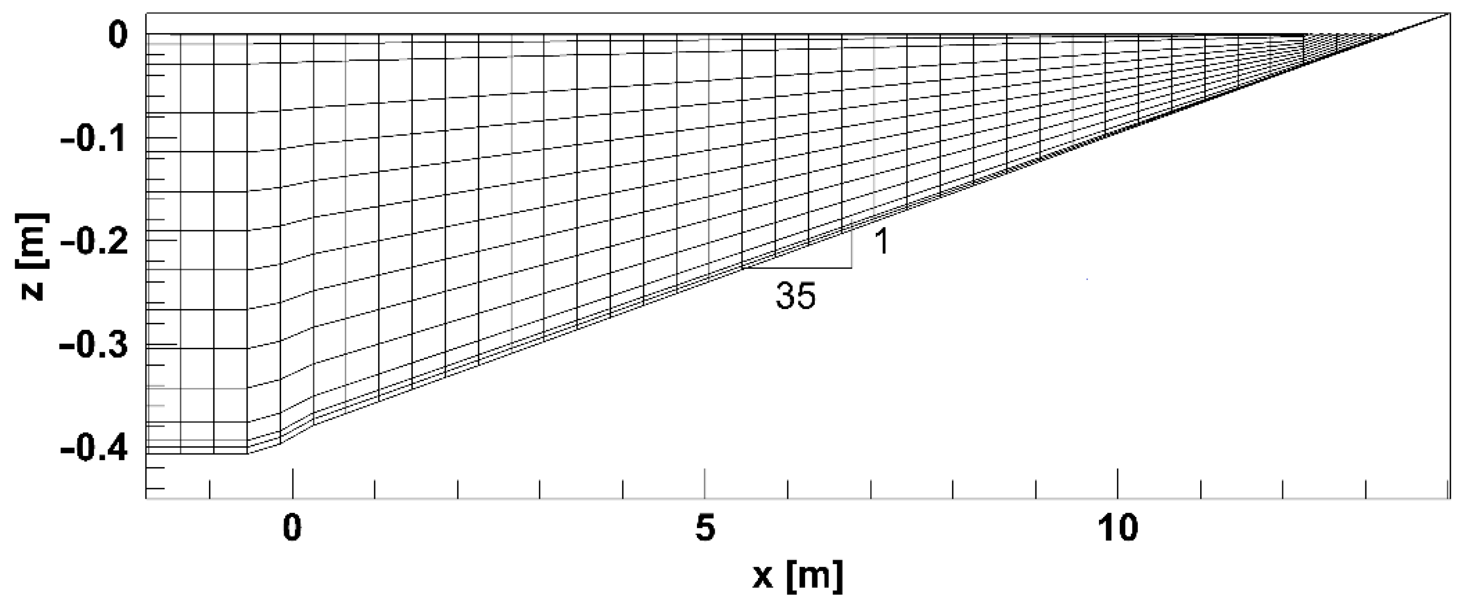
In this section, a Ting and Kirby [3] case study for a spilling breaking is numerically reproduced, in order to verify the ability of the turbulence model to represent the breaking phenomenon and turbulent phenomena that develop in the surf zone. The experimental test consists of a cnoidal wave with wave height $H_s=0.125 \mathrm{m}$, wavelength $L=6.35 \mathrm{m}$ and wave period $T=2 \mathrm{s}$, propagating in a channel with a $1:35$ seabed slope and undisturbed water at a depth of $h=0.40 \mathrm{m}$. In order to numerically reproduce the above experimental test, we use a computational grid with $512$ nodes in the horizontal direction ($\mathsf{\Delta }x=0.05 \mathrm{m}$), and $13$ non-uniformly distributed sigma layers along the vertical direction, as shown in Figure 2. At the left boundary of the computational domain, we impose the velocity components and the free-surface elevation according to the cnoidal theory by [22]. At the right boundary of the computational domain, a wet and dry technique is adopted. A no-slip boundary condition is imposed on the seabed.

The results obtained with two different numerical schemes (the low-order and new high-order numerical schemes) are presented in Section 4. Two different turbulence models (the Smagorinsky turbulence model shown in Section 3.1, and the new $k-l$ turbulence model presented in Section 3.2) are shown in this section.

The numerical simulations are made in different configurations named for the sake of simplicity as follows:

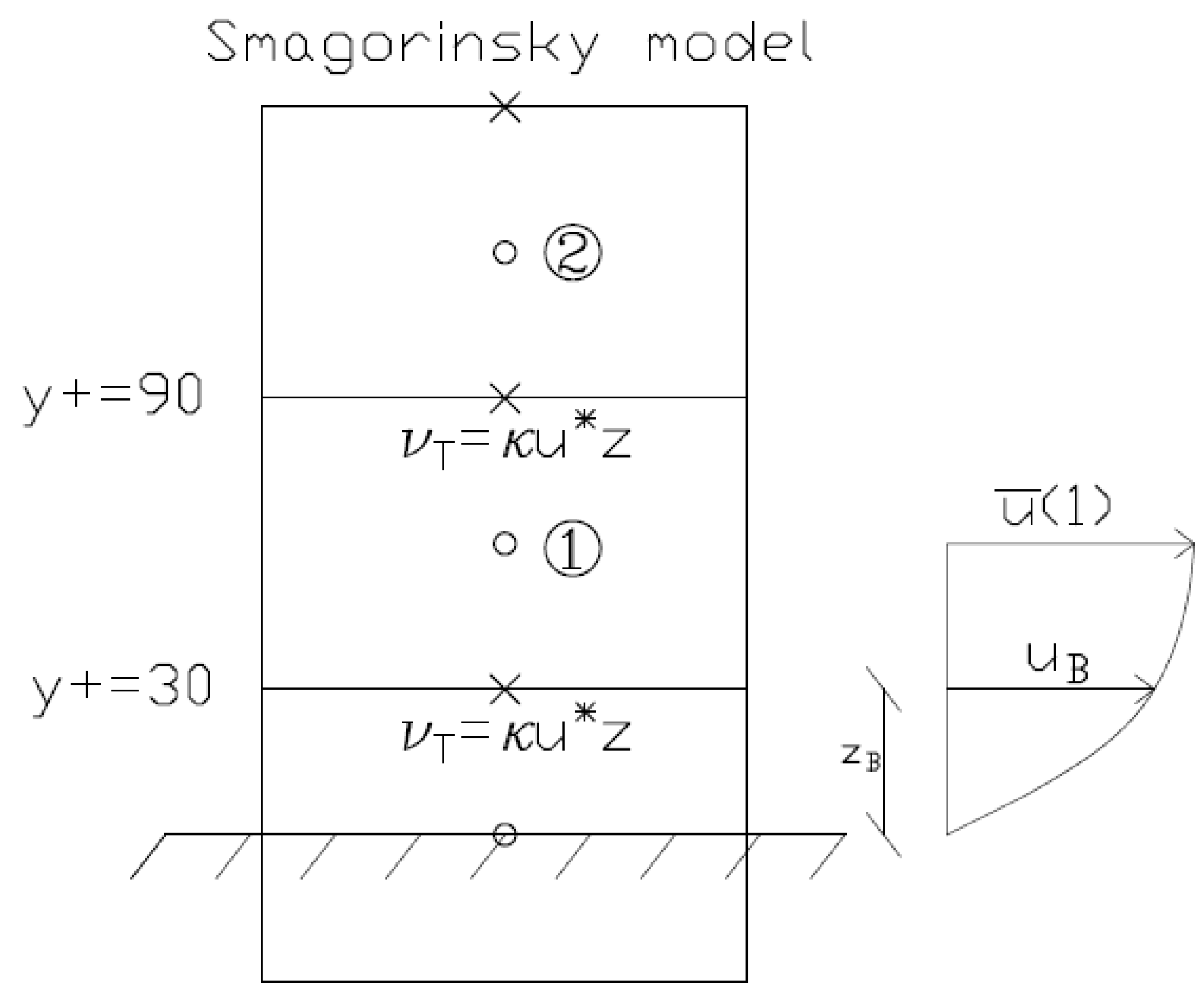
• Configuration TS. In this configuration, the eddy viscosity is expressed through the Smagorinsky model given in Section 3.1. The equations of motion are solved by the low-order numerical scheme exposed in Section 4.1 (TVD and approximate Riemann solver). In this numerical scheme, the Poisson equation is expressed in terms of primitive variables ($u^l$, and $H$). The discretization of the calculation grid cells in the turbulent boundary layer is shown in Figure 3. The first calculation grid cell (indicated with a 1 in Figure 3) in which the equations of motion are solved, is placed in the turbulent core. The boundary condition for the velocity, $u_B$, parallel to the bottom, is placed on the lower face of the first cell ($z_B$ in Figure 3), at the border between the buffer layer and the turbulent core, where $y^{+}$ is equal to $30$. The velocity boundary condition, $u_B$, is calculated by using the logarithmic law (Equation (10)) from the value of the velocity calculated at the center of the first calculation grid cell, $\overline{u},$ once the value of the friction velocity, $u^{*}$, is known. On the lower and upper faces of the first calculation grid cell (at $y^{+}=30$ and $y^{+}=90$, respectively), the eddy viscosity is calculated by using Equation (9). Outside the boundary layer ($y^{+}>90$), the Smagorinsky model is used for determining the eddy viscosity (Equation (5)).
• Configuration WS. This configuration differs from Configuration TS only by the numerical scheme: the reconstructions of the point values of the conserved variables are carried out by the WTENO technique; the time advancing of the point values of the conserved variables on the cell faces is obtained by an exact Riemann solver; the Poisson equation is expressed as a function of the conserved variables ($H{u}^l$, and $H$).
• WKC configuration. This configuration differs from Configuration WS only by the turbulence model: the eddy viscosity is expressed by the new Constant $k-l$ turbulence model (where the turbulent kinetic energy is in contravariant form) exposed in Section 3.2. In this model, the mixing length is calculated by Equation (16). The discretization of the calculation grid cells in the turbulent boundary layer is shown in Figure 4a. The first grid node in which the turbulent kinetic energy is calculated is placed on the upper face of the second calculation grid cell, indicated with a 2 in Figure 4a, in the turbulent core. On the lower face of the same calculation grid cell (at $y^{+}=90$) is placed the turbulent kinetic energy boundary condition, given by Equation (21).
• Configuration WK. This configuration differs from Configuration WKC only by the turbulence model: we propose a new turbulence $k-l$ turbulence model in which the mixing length, $l$, is calculated by Equation (17).
• Configuration WKI. This configuration differs from Configuration WK only by the discretization of the boundary layer. In order to adequately take into account the turbulent phenomena and the distribution of the turbulent kinetic energy, it is necessary to solve the equations of motion and the turbulent kinetic energy equation in the turbulent core and in the buffer layer. In this configuration, there are two calculation grid cells in the turbulent core and one also in the buffer layer. The first calculation grid cell in which the equations of motion are solved (indicated with a 1 in Figure 4b) is placed in the buffer layer. The velocity boundary condition, $u_B$, is placed on the lower face of the first calculation grid cell ($z_B$ in Figure 4b) at the border between the viscous sublayer and the buffer layer ($y^{+}=10$). On the faces of the first three calculation grid cells (up to $y^{+}=80$), the eddy viscosity is calculated by Equation (9). In order to take into account the turbulent phenomena also in the proximity of the bottom, the first grid node in which the turbulent kinetic energy is calculated is placed at the lower face of the first calculation grid cell ($y^{+}=10$). The turbulent kinetic energy boundary condition is equal to zero, and is imposed at the seabed ($y^{+}=0$). Up to $y^{+}=80$, the mixing length is given by Equation (22).

In

Table 1. Configurations.

Name	Numerical Scheme	Turbulence Model	${\mathit{y}}^{+} \mathbf{of} \mathbf{the} \mathbf{Lower} \mathbf{Face} \mathbf{of} \mathbf{the} \mathbf{First} \mathbf{Calculation} \mathbf{Grid} \mathbf{Cell}$	Vertical Layers
TS	TVD 2nd order + approximated Riemann	Smagorinsky	$y^{+}=30$	$13$
WS	WTENO + exact Riemann	Smagorinsky	$y^{+}=30$	$13$
WKC	WTENO + exact Riemann	$\mathrm{Constant} k-l$	$y^{+}=30$	$13$
WK	WTENO + exact Riemann	$k-l$ $l=l_2$	$y^{+}=30$	$13$
WKI	WTENO + exact Riemann	$k-l$ $l=l_2$	$y^{+}=10$	$18$

there is a synthetic description of the configurations.

5.1. Results Obtained by Smagorinsky Model

The numerical simulations, whose results are shown in this section, are made by the Smagorinsky turbulence model presented in Section 3.1. The numerical results obtained with the two different configurations (TS and WS) are compared with the experimental results by [3]. In both configurations, the lower face of the first calculation grid cell is placed at the border between the buffer layer and the turbulent core, at $y^{+}=30$, and the boundary conditions are assigned as shown in Figure 3.

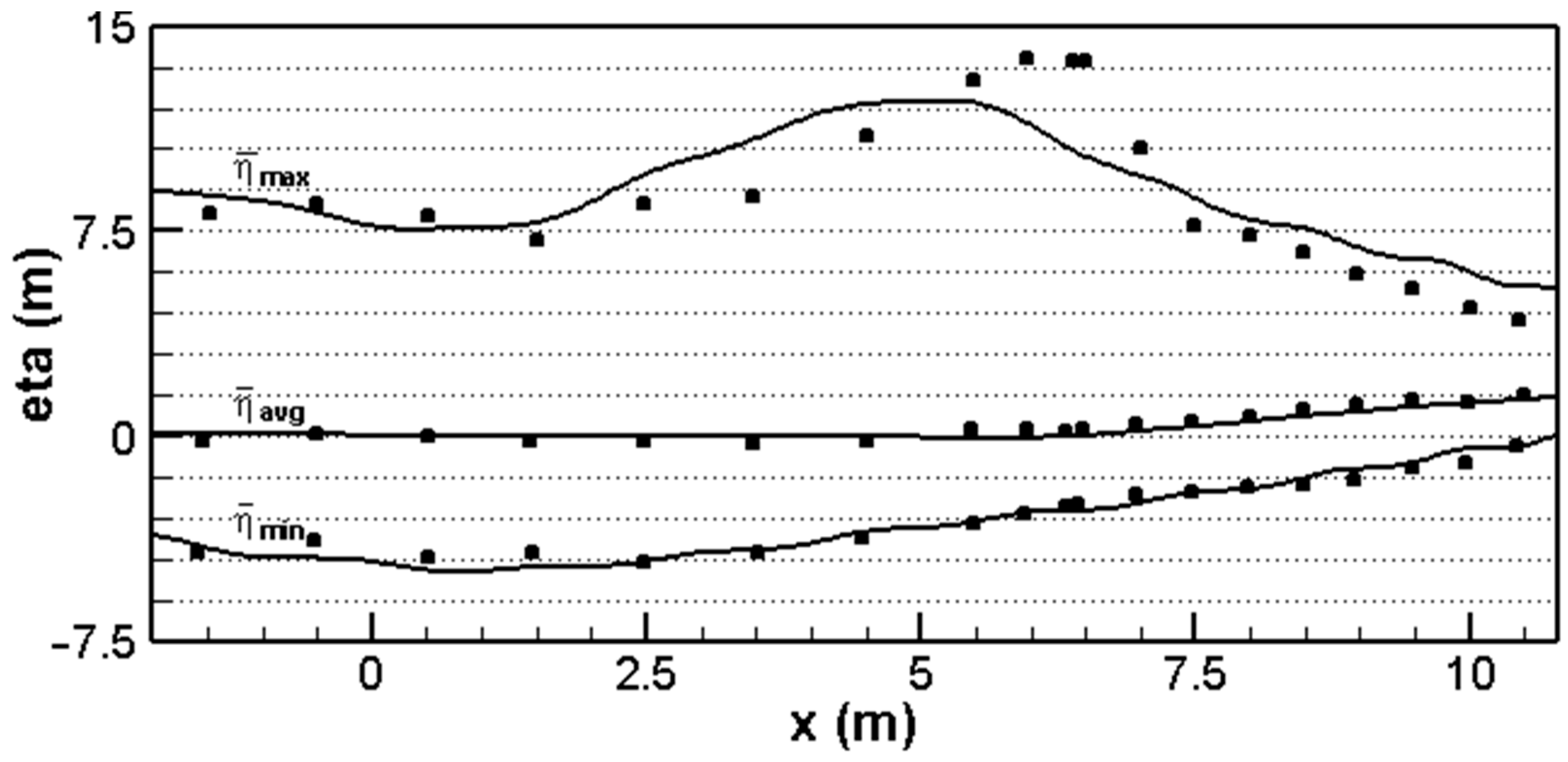
In Figure 5, the numerical results (solid line) obtained by Configuration TS with a Smagorinsky coefficient equal to $C_s=0.2$ are shown, compared with the experimental measurements (circles) in terms of the minimum, average and maximum water surface elevations.

Figure 5 shows that the maximum water surface elevation is underestimated with respect to the experimental measurements around the breaking point (Zone 2 in Figure 1); the breaking point is anticipated. The wrong position of the breaking point, shown in Figure 5, is due to the Poisson equation. Indeed, this equation is used to take into account the dynamic component of the pressure, and uses the primitive variables ($u^l$, and $H$). It is known that the use of the primitive variables produces incorrect velocity propagation of the shock [13]. The underestimation of the maximum water surface elevation is due to the shock-capturing numerical scheme used: this is a low-order numerical scheme that has the task of dissipating the largest part of the kinetic energy of averaged motion. The adopted low-order scheme limits spurious oscillations that are generated in proximity of the shock by using TVD reconstruction techniques (from the cell average values to the point ones) that are no higher than second order. This scheme allows us to have second-order accuracy where the solution is regular, while it limits spurious oscillations by reducing the order of accuracy in proximity to discontinuities. The additional reason that too much dissipation of kinetic energy of the averaged motion is produced (as we can see in Figure 5) is due to the use (in Configuration TS) of an approximate Riemann solver. The solver only considers in the solution the shock and rarefaction waves, and does not consider the contact waves. In the presence of shock, the incomplete solution produces an excess in numerical dissipation of kinetic energy of the averaged motion.

From Figure 5 it is clear that the low-order numerical scheme, which uses an approximate Riemann solver, is less accurate; it anticipates the breaking point and introduces an excess dissipation of kinetic energy of the averaged motion, producing an underestimation of the wave height and of the maximum water surface elevation around the breaking point (Zone 2 in Figure 1). It is necessary to overcome these limits and develop a new high-order shock-capturing numerical scheme. High-order schemes, in general, introduce less numerical dissipation and allow us to attribute the right quantity of dissipated kinetic energy of the averaged motion mainly to the turbulence model, in order to adequately represent the turbulent agitations that affect the resuspension of the sediments.

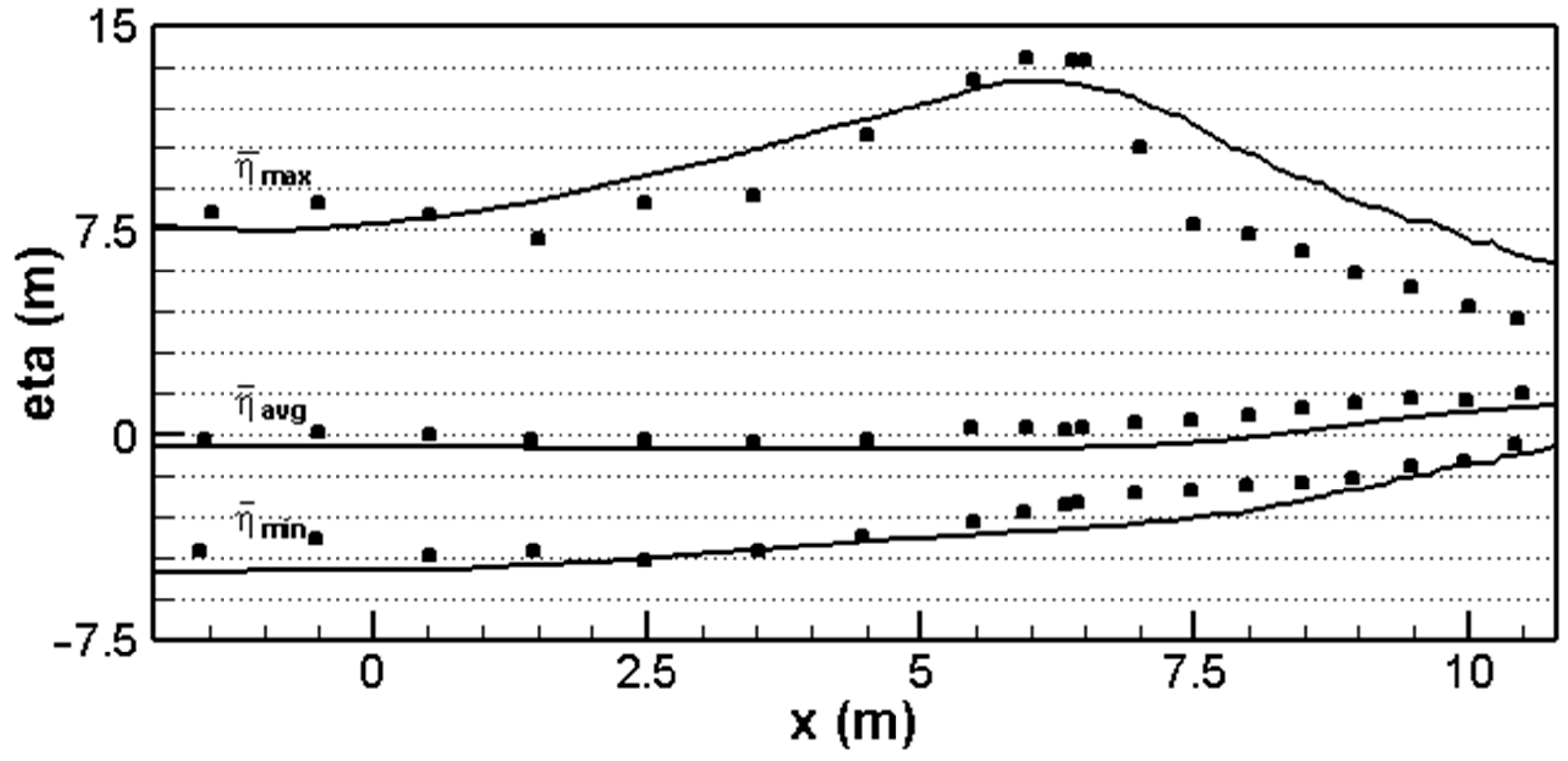
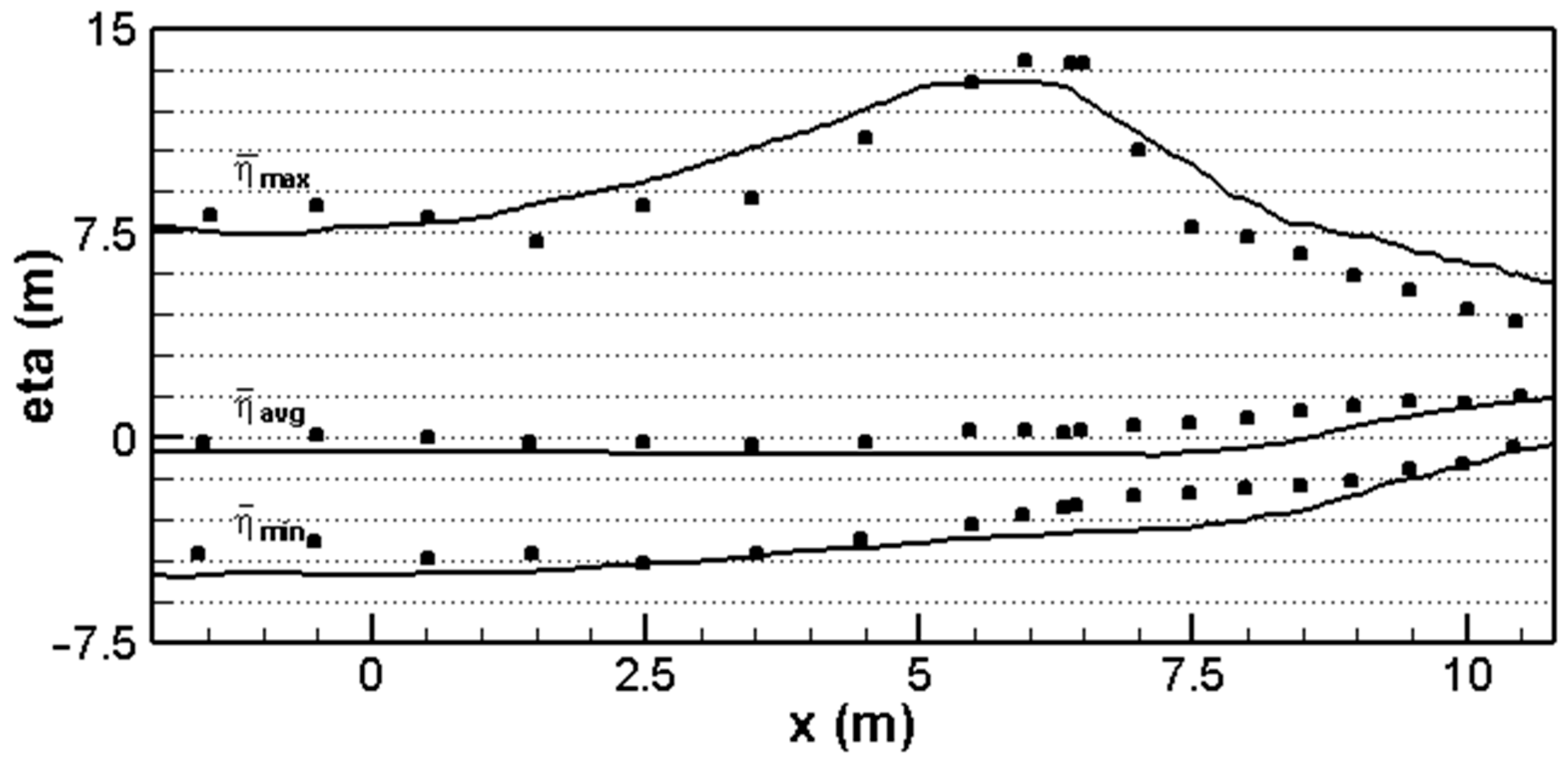
Figure 6 and Figure 7 show the numerical results obtained by Configuration WS, in which the turbulence model is the same as that used in Configuration TS; the numerical scheme is the high-order one proposed in this paper.

From Figure 6 it can be seen that the breaking point is slightly anticipated with respect to the one obtained by the experimental measurements; the maximum water surface elevation around the breaking point (Zone 2 in Figure 1) is slightly underestimated, while in the surf zone (Zones 3 and 4 in Figure 1) the maximum water surface elevation is overestimated with respect to the experimental one. It is evident from Figure 5 and Figure 6 that the proposed high-order numerical scheme (using an exact Riemann solver, fifth- order WTENO reconstructions and conserved variables also in the Poisson equation) allows us to limit the excessive numerical dissipation of the averaged motion introduced by the low-order numerical scheme.

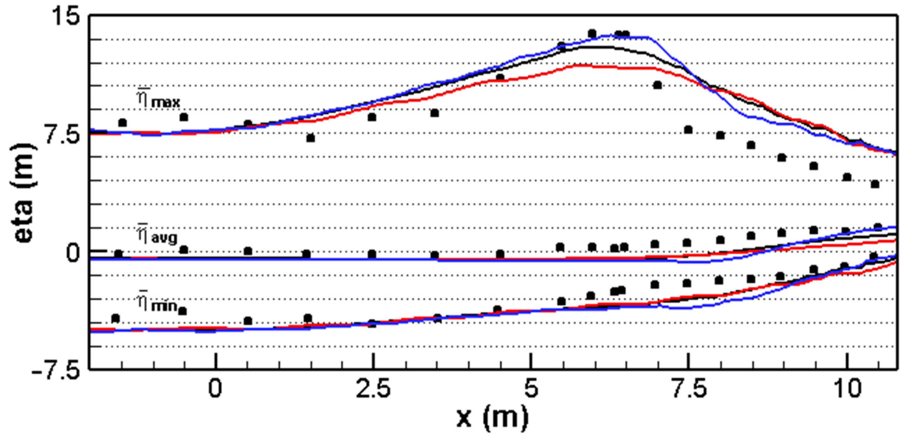
In Figure 7, the numerical results obtained with the same turbulence model of Configuration TS and three different Smagorinsky coefficients in Configuration WS, $C_s=0.1, 0.2$, and $0.3$ are shown, but also includes the new high-order numerical scheme presented in this paper (Configuration WS).

The comparison between the three different simulations shows that when the Smagorinsky coefficient increases (i.e., from the blue line to the red one) in the shoaling zone (Zone 1 in Figure 1) and around the breaking point, the maximum water surface elevation is overall underestimated; consequently, the turbulence model increases the dissipation of energy of the averaged motion. Increasing the eddy viscosity increases the reduction in the maximum wave height. As shown in Figure 7, the numerical results are strongly influenced by the choice of the Smagorinsky coefficient. In all three simulations, the maximum water surface elevation is overestimated in the surf zone (Zones 3 and 4 in Figure 1). The overestimation of the maximum water surface elevation is considered dependent on a high value of the eddy viscosity, as calculated by the Smagorinsky model. A high value of this coefficient produces diffusion in the motion direction of the momentum, and this means that the steepness of the breaking wave fronts is reduced, and that the maximum water surface elevation is high. From the previous consideration, it can be seen that the capability of the Smagorinsky model in representing the turbulent phenomena as well as their effects on the dissipation of kinetic energy of the averaged motion in the surf zone (Zones 3 and 4 in Figure 1) is limited. Consequently, a new turbulence model $k-l$, presented in Section 3.2 with an equation for the turbulent kinetic energy, is proposed in order to overcome the above-mentioned limits.

5.2. Results Obtained by $k-l$ Model

The numerical simulations, whose results are shown in this section, are made by the $k-l$ turbulence model in three different configurations: WKC, WK and WKI. As already mentioned in the descriptions of these configurations, the new numerical scheme which has fifth-order reconstructions, an exact Riemann solver and conserved variables also in the Poisson equation, is used.

In Figure 8, the numerical results obtained with the new Constant $k-l$ turbulence model presented in Section 3.2 (in which the mixing length is given by the Equation (16)) (Configuration WKC) are shown and compared with the experimental results. In this configuration, the lower face of the first calculation grid cell is collocated between the buffer layer and the turbulent core, $y^{+}=30$, and the boundary conditions are assigned as shown in Figure 4a.

From the comparison between the numerical and experimental results, it can be seen that the new Constant $k-l$ model slightly underestimates the maximum water surface elevation at the breaking point, and anticipates the breaking point. The new Constant $k-l$ does not vary the value of the mixing length, $l$, in the different zones; thus, it does not vary the eddy viscosity nor the viscous dissipation of the turbulent kinetic energy in the zones, i.e., in the shoaling zone (Zone 1 in Figure 1), around the breaking point (Zone 2 in Figure 1), in the surf zone (Zones 3 and 4 in Figure 1) and in proximity of the bottom (Zone 5 in Figure 1). The effect produced by the mixing length in the new Constant $k-l$ in Zones 3 and 4 can be summarized by an increase in the diffusion in the motion direction of the average momentum, with a consequent reduction in the slope of the envelope line of the maximum water surface elevation with respect to the experimental results.

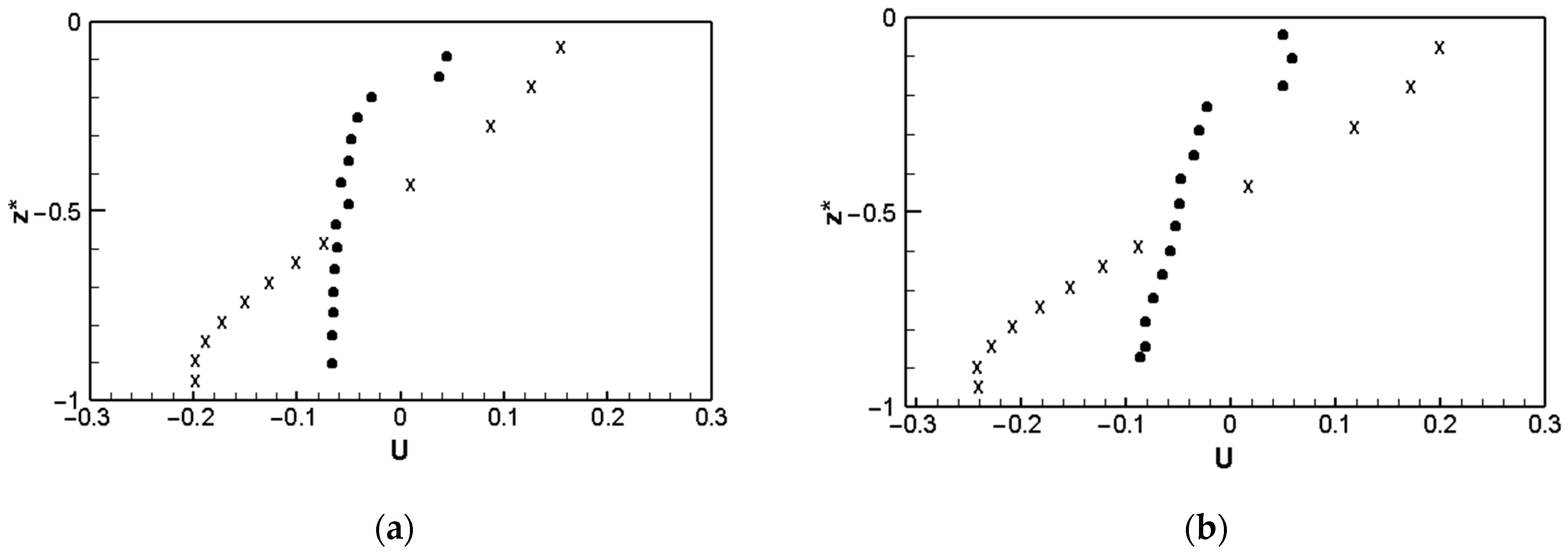
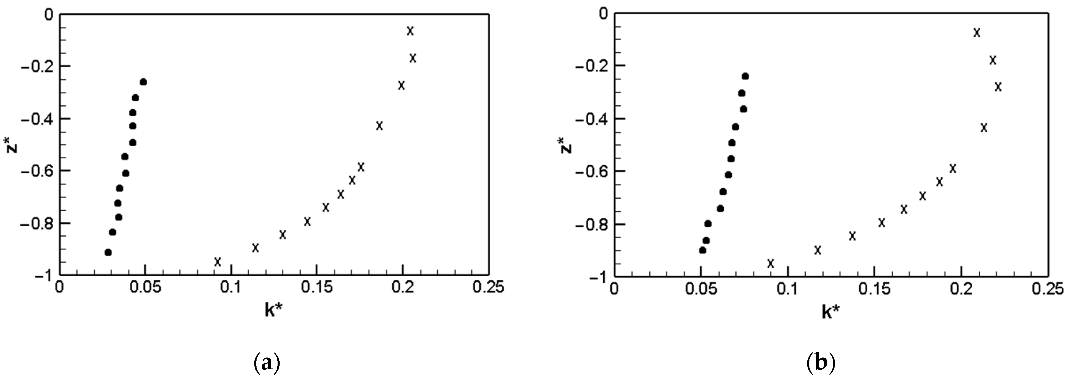
Figure 9 and Figure 10 show the time mean vertical distribution of the turbulent kinetic energy and horizontal velocity at $x=7.27 \mathrm{m}$ and $x=7.88 \mathrm{m}$.

The vertical distribution of turbulent kinetic energy in Configuration WKC is overestimated with respect to the experimental measurements, as shown in Figure 9. The vertical distribution of the time mean horizontal velocity, shown in Figure 10, is characterized by the fact that the velocity near the bottom is offshore directed, while near the free surface it is onshore directed. This particular mean horizontal flow is called undertow. In Figure 10, the undertow obtained by the numerical simulation is overestimated.

The comparison between the experimental and the numerical results obtained by the new Constant $k-l$ model (in which the mixing length is given by Equation (16)), shows that it is necessary to further reduce the effects produced by an excess of the diffusion in the motion direction of the average momentum, in order to increase the slope of the envelope line of the maximum water surface elevation.

A new $k-l$ model (presented in Section 3.2) is proposed; in this model, the mixing length is calculated as a function of the spatial variation of the maximum water surface elevation and its second derivative. In Figure 11, the numerical results obtained with the new $k-l$ model are shown. The lower face of the first calculation grid cell is placed at $y^{+}=30$ away from the wall (Configuration WK), as was done with the previous Configuration WKC.

From the comparison between the experimental and numerical results shown in Figure 11, it is deduced that the new turbulence model increases (even if insufficiently) the steepness of the maximum water surface elevation after the breaking point (Zone 3 in Figure 1) with respect to the steepness in Figure 8. Figure 12 and Figure 13 show the time mean turbulent kinetic energy and undertow profiles at $x=7.27 \mathrm{m}$ and $x=7.88 \mathrm{m}$.

From Figure 12 and Figure 13, it is evident that also in this configuration the vertical distribution of turbulent kinetic energy and undertow are overestimated with respect to the experimental measurements. In the buffer layer and in the turbulent core in the bottom boundary layer, there is significant production of turbulent kinetic energy, as well as a strong variability in it along the vertical direction. The above-mentioned production in the turbulent core and in the buffer layer influence the vertical distribution of the turbulent kinetic energy. It is necessary (see Figure 13) to solve the equations of motion in addition to the turbulent kinetic energy equation in the turbulent core, and also in the buffer layer, in order to adequately represent the distribution of the turbulent kinetic energy nearer to the seabed. The turbulent kinetic energy equation is solved from $y^{+}=10$, and the equations of motion are solved in the buffer layer.

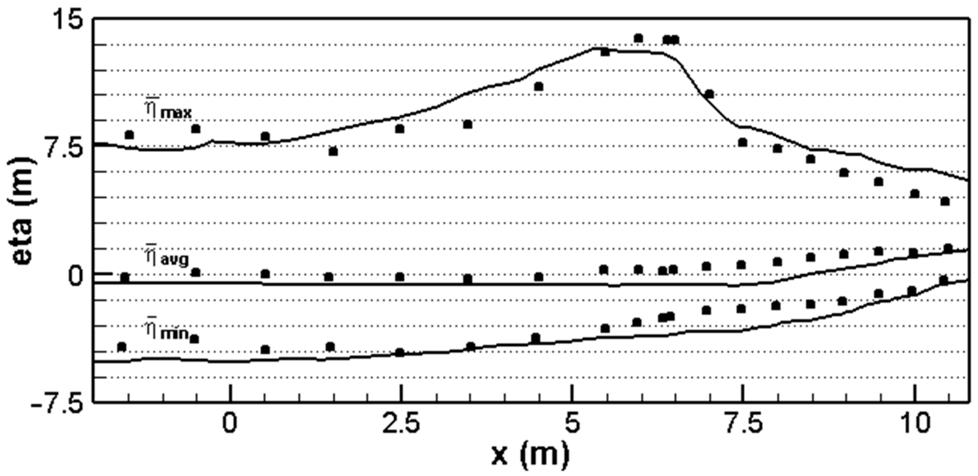
Figure 14 shows the numerical results obtained with the new turbulence model, in which the lower face of the first calculation grid cell is placed at $y^{+}=10$ (Configuration WKI). The discretization of the calculation grid cells inside the boundary layer, in addition to the boundary conditions, are shown in Figure 4b.

In Configuration WKI, the breaking point is well predicted, and the maximum water surface elevation is in good agreement with the experimental results.

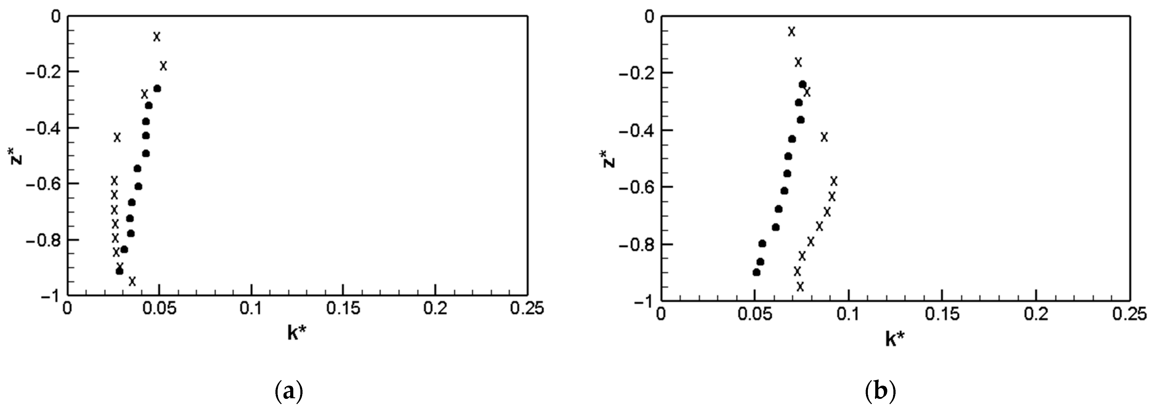
In Figure 15, the time mean turbulent kinetic energy distribution along the vertical direction is shown. The first calculation grid cell in the buffer layer produced numerical results that were in good agreement with the experimental results, as shown in Figure 15. From Figure 16, it can be seen, moreover, that the time mean undertow profiles are in good agreement with the experimental profiles at $x=7.27 \mathrm{m}$; meanwhile, at $x=7.88 \mathrm{m}$ the velocity at the free surface and at the bottom are slightly overestimated.

By comparing Figure 15 and Figure 16, it is evident that solving the equations of motion in the buffer layer and for the turbulent kinetic energy at the border between the viscous sublayer and the buffer layer allows us to more accurately represent the turbulent phenomena in the boundary layer. In this way, it is possible to achieve good agreement between the numerical and experimental results in terms of turbulent kinetic energy and undertow profiles.

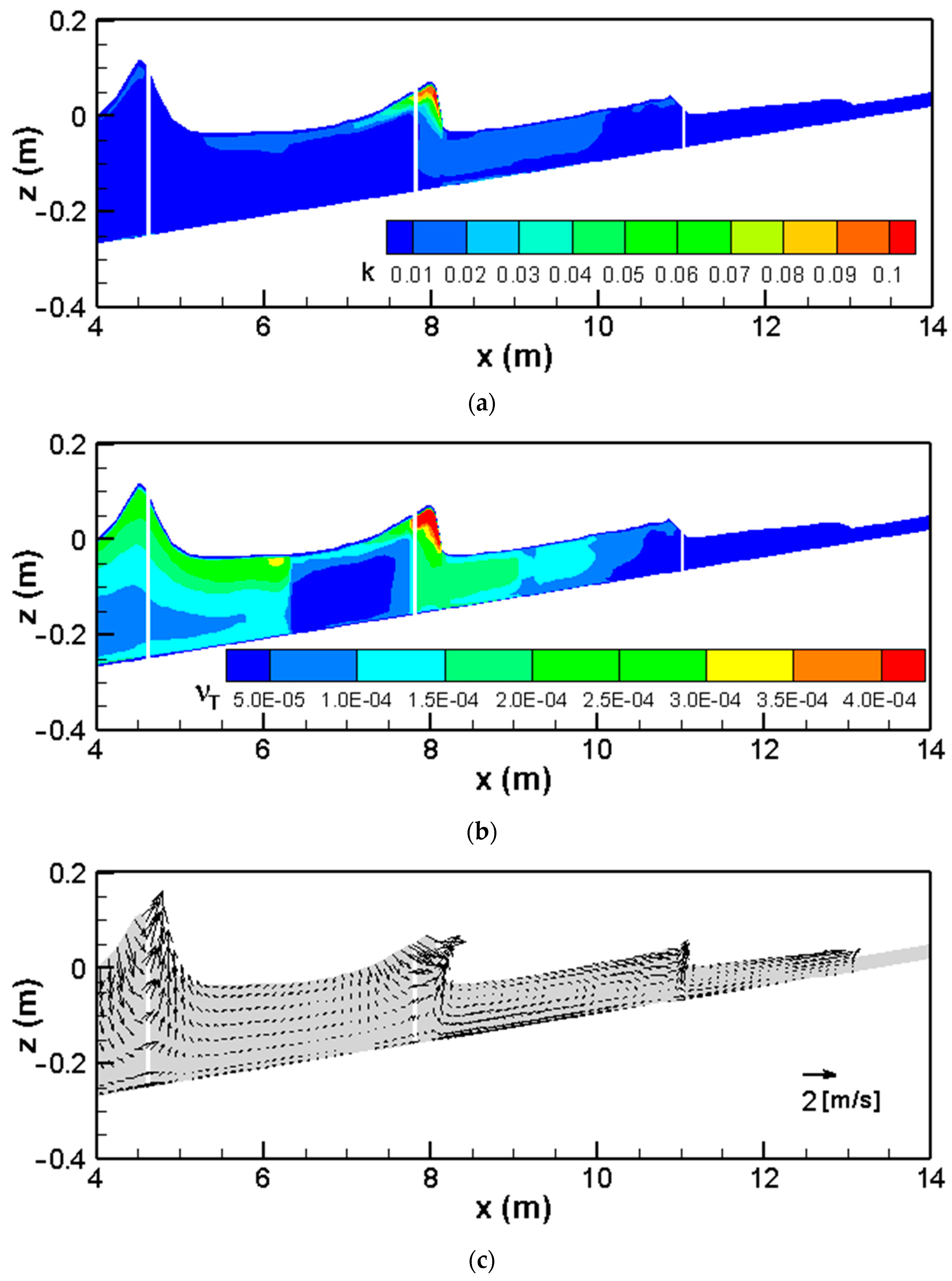
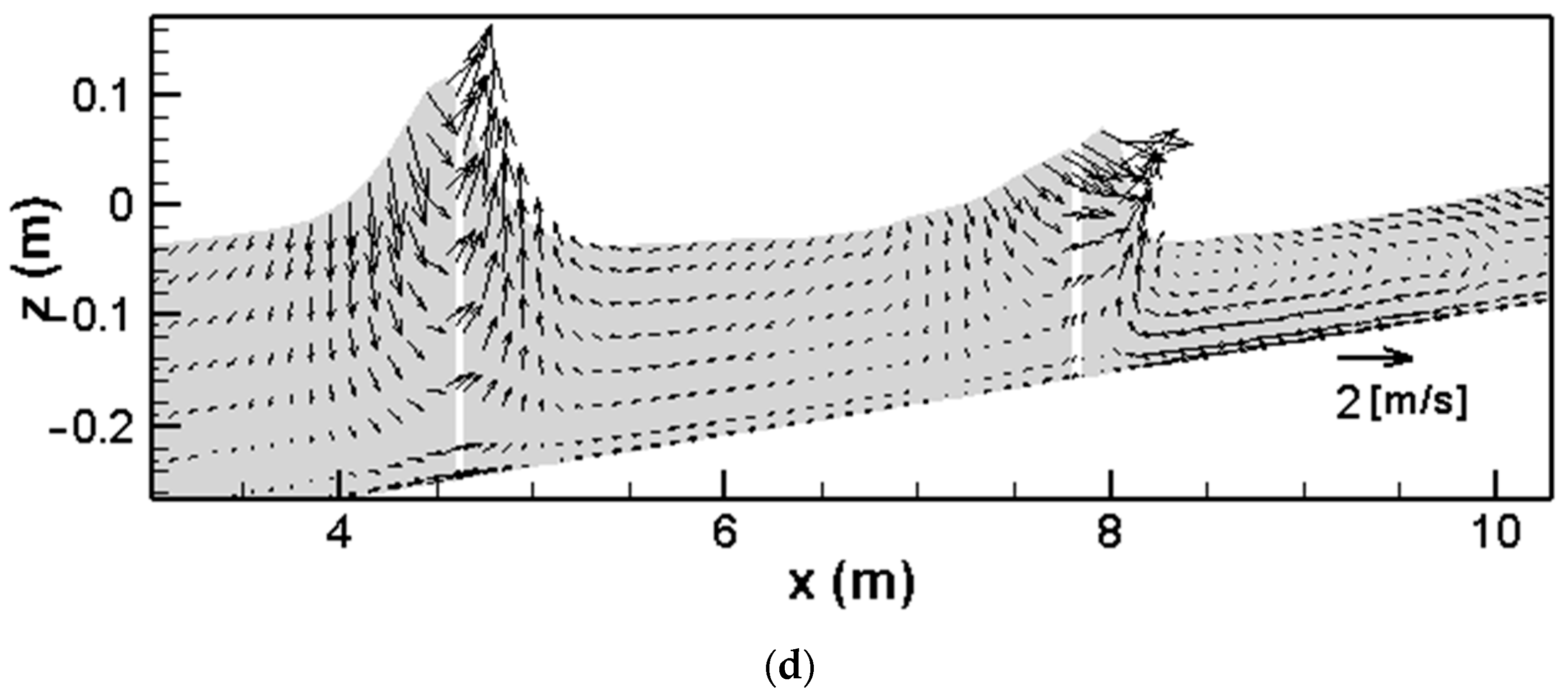
In Figure 17a,b, instantaneous wave fields of turbulent kinetic energy and eddy viscosity at time $t=98.75 \mathrm{s}$ are shown. The greater values of the turbulent kinetic energy and eddy viscosity are produced on the breaking wave fronts. On these fronts, the WTENO reconstructions significantly reduce the numerical dissipation of energy of the average motion, entrusting to the turbulence model the task of dissipating the right quantity of this energy. From Figure 17b it can be seen that the eddy viscosity is reduced in Zone 3 ($x\cong 6.5 \mathrm{m}-7.5 \mathrm{m}$) because the mixing length (Equation (17)) reduces its value in this zone. Figure 17c,d represent, respectively, an instantaneous velocity field and a zoom of the same velocity field in which one vector out of every two is shown at the same time, $t=98.75 \mathrm{s}$.

6. Conclusions

In this paper, the hydrodynamic and free-surface elevation fields in breaking waves are simulated by solving the integral and contravariant forms of the three-dimensional Navier–Stokes equations expressed in a generalized time-dependent curvilinear coordinate system, in which the vertical coordinate moves by following the free surface.

A new $k-l$ turbulence model in contravariant form is proposed; in this model, the mixing length, $l$, is defined as a function of the maximum water surface elevation spatial variation. A new original numerical scheme is proposed based on three elements of originality. The first element of originality consists of expressing the Poisson equation in terms of conserved variables. The second element is to propose a new fifth-order reconstruction technique of the point values of conserved variables, named in this paper as WTENO, that allows us to modify the polynomials choice in a dynamic way. The third element of originality is the use of an exact Riemann solver.

In this paper, it has been demonstrated that the Smagorinsky turbulence model, which uses a low-order numerical scheme, produces an excess dissipation in kinetic energy of average motion. The proposed high-order numerical scheme, the new $k-l$ turbulence model in contravariant formulation (with a mixing length, $l$, and functions of the spatial variation of the maximum water surface elevation) and the refinement in the bottom boundary layer of the gird cells allow us to achieve numerical results that are in good agreement with respect to the experimental results in terms of the maximum water surface elevation, the vertical distribution of turbulent kinetic energy, and the undertow.

References

- De Serio, F.; Mossa, M. A laboratory study of irregular shoaling waves. Exp. Fluids 2013, 54, 1536. [Google Scholar] [CrossRef]
- De Serio, F.; Mossa, M. Experimental observations of turbulent events in the surfzone. J. Mar. Sc. Eng. 2019, 7, 332. [Google Scholar] [CrossRef] [Green Version]
- Ting, F.C.K.; Kirby, J.T. Observation undertow and turbulence in a wave period. Coast. Eng. 1995, 24, 177–204. [Google Scholar] [CrossRef]
- De Padova, D.; Mossa, M.; Sibilla, M. SPH numerical investigation of the velocity field and vorticity generation within a hydrofoil-induced spilling breaker. Environ. Fluid Mech. 2016, 16, 267–287. [Google Scholar] [CrossRef]
- De Padova, D.; Meftah, M.B.; De Serio, F.; Mossa, M. Characteristics of breaking vorticity in spilling and plunging waves investigated numerically by SPH. Environ. Fluid Mech. 2020, 20, 233–260. [Google Scholar] [CrossRef]
- Kazolea, M.; Delis, A.I. A well-balance shock-capturing hybrid finite volume-finite difference numerical scheme for extended 1D Boussinesq models. Appl. Numer. Math. 2013, 67, 167–186. [Google Scholar] [CrossRef] [Green Version]
- Kazolea, M.; Delis, A.I.; Synolakis, C.E. Numerical treatment of wave breaking on unstructured finite volume approzimation for extended Boussinesq-type equations. J. Comput. Phys. 2014, 271, 281–305. [Google Scholar] [CrossRef]
- Kozyrakis, G.V.; Delis, A.I.; Alexandrakis, G.; Kampanis, N.A. Numerical modeling of sediment transport applied to coastal morphodynamics. Appl. Numer. Math 2016, 104, 30–46. [Google Scholar] [CrossRef]
- Ma, G.; Shi, F.; Kirby, J.T. Shock-capturing non-hydrostatic model for fully dispersive surface wave processes. Ocean Model. 2012, 43–44, 22–35. [Google Scholar] [CrossRef]
- Cannata, G.; Petrelli, C.; Barsi, L.; Gallerano, F. Numerical integration of the contravariant integral form of the Navier–Stokes equations in time-dependent curvilinear coordinate systems for three-dimensional free surface flows. Contin. Mech. Thermodyn. 2019, 31, 491–519. [Google Scholar] [CrossRef] [Green Version]
- Cannata, G.; Palleschi, F.; Iele, B.; Cioffi, F. A three-dimensional numerical study of wave induced currents in Cetraro Harbour coastal area (Italy). Water 2020, 12, 935. [Google Scholar] [CrossRef] [Green Version]
- Bradford, S.F. Numerical simulation of surf zone dynamics. J. Waterw. Port Coast. Ocean Eng. 2000, 126, 1–13. [Google Scholar] [CrossRef]
- Toro, E.F. Shock-Capturing Methods for Free-Surface Shallow Flows; Wiley: New York, NY, USA, 2001. [Google Scholar]
- Phillips, N.A. A coordinate system having some special advantages for numerical forecasting. J. Meteorol. 1957, 14, 184–185. [Google Scholar] [CrossRef] [Green Version]
- Liu, P.L.F.; Lin, P. A numerical model for breaking waves: The volume of fluid method. Research Report No. CACR-97-02. J. Fluid Mech. 1997, 359, 56. [Google Scholar]
- Cannata, G.; Gallerano, F. A dynamic two-equation sub grid scale model. Continuum Mech. Thermodyn. 2005, 17, 101–123. [Google Scholar] [CrossRef]
- Jiang, G.; Shu, C. Efficient Implementation of Weighted ENO Schemes. J. Comput. Phys. 1996, 126, 202–228. [Google Scholar] [CrossRef] [Green Version]
- Peng, J.; Liu, S.; Li, S.; Zhang, K.; Shen, Y. An efficient targeted ENO scheme with local adaptive dissipation for compressible flow simulation. J. Comput. Phys. 2021, 425, 109902. [Google Scholar] [CrossRef]
- Liu, X.; Duncan, J. An experimental study of surfactant effects on spilling breakers. J. Fluid Mech. 2006, 567, 433–455. [Google Scholar] [CrossRef]
- Liu, X.; Duncan, J. Weakly breaking waves in the presence of surfactant micelles. Phys. Rev. E 2007, 76, 061201-1–061201-5. [Google Scholar] [CrossRef]
- Stagonas, D.; Warbrick, D.; Muller, G.; Magagna, D. Surface tension effects on energy dissipation by small scale, experimental breaking waves. Coast. Eng. 2011, 58, 826–836. [Google Scholar] [CrossRef]
- Weigel, R. A presentation of cnoidale wave theory for practical application. J. Fluid. Mech. 1960, 7, 273–286. [Google Scholar] [CrossRef] [Green Version]
Figure 1.
Maximum, averaged and minimum water surface elevations. Definitions of the zones.
Figure 2.
Computational domain (only one line out of every six is drawn in the horizontal direction).
Figure 3.
Discretization of the vertical cells outside the buffer layer for the Smagorinsky model.
Figure 4.
Discretization of the vertical cells outside the buffer layer (a) and inside the buffer layer (b) for the model.
Figure 5.
Results 1: minimum, average and maximum water surface elevations in Configuration TS, showing numerical results (solid line) and experimental measurements (circles).
Figure 6.
Results 2: minimum, average and maximum water surface elevations in Configuration WS, showing numerical results (solid line) and experimental measurements (circles) [3].
Figure 7.
Results 3: minimum, average and maximum water surface elevations in Configuration WS, showing numerical results (blue solid line , black solid line , red solid line ) and experimental measurements (circles) [3].
Figure 8.
Results 4: minimum, average and maximum water surface elevations in Configuration WKC, showing numerical results (solid line) and experimental measurements (circles) [3].
Figure 9.
Result 4: time mean turbulent kinetic energy profiles in Configuration WKC, showing numerical results (X) and experimental results (circles) [3]. (a) (b) , and .
Figure 10.
Result 4: undertow profiles in Configuration WKC, showing numerical results (X) and experimental results (circles) [3]. (a) (b) , and ; and .
Figure 11.
Results 5: minimum, average and maximum water surface elevations in Configuration WK., showing numerical results (solid line) and experimental measurements (circles) [3].
Figure 12.
Result 5: time mean turbulent kinetic energy profiles in Configuration WK, showing numerical results (X) and experimental results (circles) [3]. (a) (b) , and .
Figure 13.
Result 5: undertow profiles in Configuration WK, showing numerical results (X) and experimental results (circles) [3]. (a) (b) , and ; and .
Figure 14.
Results 6: minimum, average and maximum water surface elevations in Configuration WKI, showing numerical results (solid line) and experimental measurements (circles) [3].
Figure 15.
Results 6: time mean turbulent kinetic energy profiles in Configuration WKI, showing numerical results (X) and experimental results (circles) [3]. (a) (b) , and .
Figure 16.
Result 6: undertow profiles in Configuration WKI, showing numerical results (X) and experimental results (circles) [3]. (a) (b) , , and ; and .
Figure 17.
Results 6: instantaneous wave fields in Configuration WKI. (a) Turbulent kinetic energy contour, (b) eddy viscosity contour, (c) velocity fields (one vector out of every two is shown) and (d) zoom of velocity fields at .