
Experimental and Numerical Study on Vortical Structures and Their Dynamics in a Pump Sump


1
Institute of Thermomechanics, Czech Academy of Sciences, Dolejškova 1402/5, 182 00 Praha, Czech Republic
2
Department of Power System Engineering, Faculty of Mechanical Engineering, University of West Bohemia, Universitní 22, 306 14 Plzeň, Czech Republic
3
Centre of Hydraulic Research, Jana Sigmunda 313, 783 49 Lutín, Czech Republic
*
Author to whom correspondence should be addressed.
Water 2022, 14(13), 2039; https://doi.org/10.3390/w14132039
Submission received: 26 April 2022
/
Revised: 7 June 2022
/
Accepted: 22 June 2022
/
Published: 25 June 2022
(This article belongs to the Topic Hydroelectric Power)
Abstract
:Research on water flow in a pump inlet sump is presented. The main effort has been devoted to the study of the vortical structures’ appearance and their behavior. The study was conducted in a dedicated model of the pump sump consisting of a rectangular tank 1272 × 542 × 550 mm3 with a vertical bellmouth inlet 240 mm in diameter and a close-circuit water loop. Both Computational Fluid Dynamics (CFD) and experimental research methods have been applied. The advanced unsteady approach has been used for mathematical modeling to capture the flow-field dynamics. For experiments, the time-resolved Particle Image Velocimetry (PIV) method has been utilized. The mathematical modeling has been validated against the obtained experimental data; the main vortex core circulation is captured within 3%, while the overall flow topology is validated qualitatively. Three types of vortical structures have been detected: surface vortices, wall-attached vortices and bottom vortex. The most intense and stable is the bottom vortex; the surface and wall-attached vortices are found to be of random nature, both in their appearance and topology; they appear intermittently in time with various topologies. The dominant bottom vortex is relatively steady with weak, low-frequency dynamics; typical frequencies are up to 1 Hz. The origin of the vorticity of all large vortical structures is identified in the pump propeller rotation.
1. Introduction
Nowadays, hydropower systems are getting much more important since modern society feels the need for sustainable and reliable sources of energy. For example, a hydroelectric power station generates two orders of magnitude less greenhouse gases in comparison with classical power sources ([1]). The hydropower share of the global electricity market is about 17%. On the other hand, the pump, which can be used to maintain the desirable flood level, should also operate with maximal achievable efficiency. This task is quite hard to fulfill, especially for off-design operational conditions. The efficiency of hydraulic machines is very sensitive to the existence of vortex cores entering the propeller. The free surface vortices are unacceptable phenomena, in particular, their existence is proportionally dependent on the value of submergence, and they bring many unwanted aspects, such as rotational flow, cavitation effect and, worse, the air entrainment from the free surface. Changing the flow rate or increasing the submergence value is the typical measure to avoid these vortices. The critical value of submergence depends on various parameters such as intake velocity V, intake diameter D, geometry of the intake bellmouth, circulation value Γ, gravity acceleration g, density of medium ρ, surface tension σ, viscosity of medium ν, etc. The submerged vortices occur as a consequence of the pressure drop from the pump suction. Unlike the free surface vortices, the presence of the submerged vortices is not directly related to the submergence value; still, submergence can influence the cavitation state in the submerged vortex core. Anti Vortex Devices (AVD) could be utilized as a passive control method [2,3]; they can disrupt the angular momentum of the flow and thus suppress the vortices.
This paper deals with the flow phenomena in a pump sump using experimental and numerical methods. The three types of vortices that can enter the impeller inlet are under study: free surface vortices, wall-attached vortices and bottom vortex.
The free surface vortices, also known as air-entrained vortices [4], are studied very often. A total of 1% air entering the pump impeller can cause a rapid decrease in the hydraulic efficiency, and even higher amounts of gaseous components can lead to high bearing loading and could result in serious damage to the pump [5]. There are six levels of classification of the surface vortices [1]: (1) coherent surface swirl; (2) surface dimple; (3) dye core to intake; (4) vortex pulling floating trash; (5) vortex pulling air bubbles; (6) full air core to intake. The higher the level, the more dangerous.
Wall-attached vortices, also known as submerged vortices, are the side vortices and the bottom vortex. Both wall-attached and bottom vortices enter the impeller hub, the first one is attached to the side wall, and the second one is connected to the bottom just below the pump inlet. The connection with the wall can be modeled by a singular point.
It is highly useful to know the operating conditions when these phenomena take place, and then we could try to prevent their formation. For this reason, the flow topology in space and time are examined numerically and experimentally. Due to financial costs, CFD methods predominate, see [6,7,8,9,10,11,12,13,14]. Experimental studies of suction pumps in a sump can be found seldom in the literature, and if so, the experimental methods are based on the visualization technique [5,6] or the measurement of the swirl angle of a pump-approaching flow [7]. Planar velocity fields can be inspected using the Particle Image Velocimetry (PIV) method effectively [3,4]. To the best of our knowledge, almost no relevant literature has been published on the free surface or bottom vortex dynamics; the time-averaged data are presented as a rule.
Obviously, the published information relative to the intake objects of a pump is very limited. We are going to use the knowledge gained during the project on discharge objects [8]. However, there are numerous substantial differences between these two types of flow. In the intake, vortices are primarily driven due to the presence of the rotating impeller, which causes the swirl. This driving mechanism is common for the vortical structures emerging in this case.
The main goal of the presented paper is the investigation of the vortex structures typical for the pump intake configuration, the surface and bottom vortices, in particular. The main method to study the flow topology and flow dynamics are PIV in the experimental part and the CFD solver ANSYS CFX in mathematical modeling. The numerical tool is to be validated and verified. We will put emphasis on dominant flow structures, their topology and time characteristics in those processes. Hence, the physical model was designed and fabricated to allow optical measurement with maximal possible accuracy. To study the flow-field dynamics, advanced decomposition methods such as Proper Orthogonal Decomposition (POD) and Oscillation Pattern Decomposition (OPD) are to be used to extract the dominant dynamic modes and to determine distinct frequencies presented in the flow. For more details on POD and OPD methods, see [15,16].
2. Test Case Setup
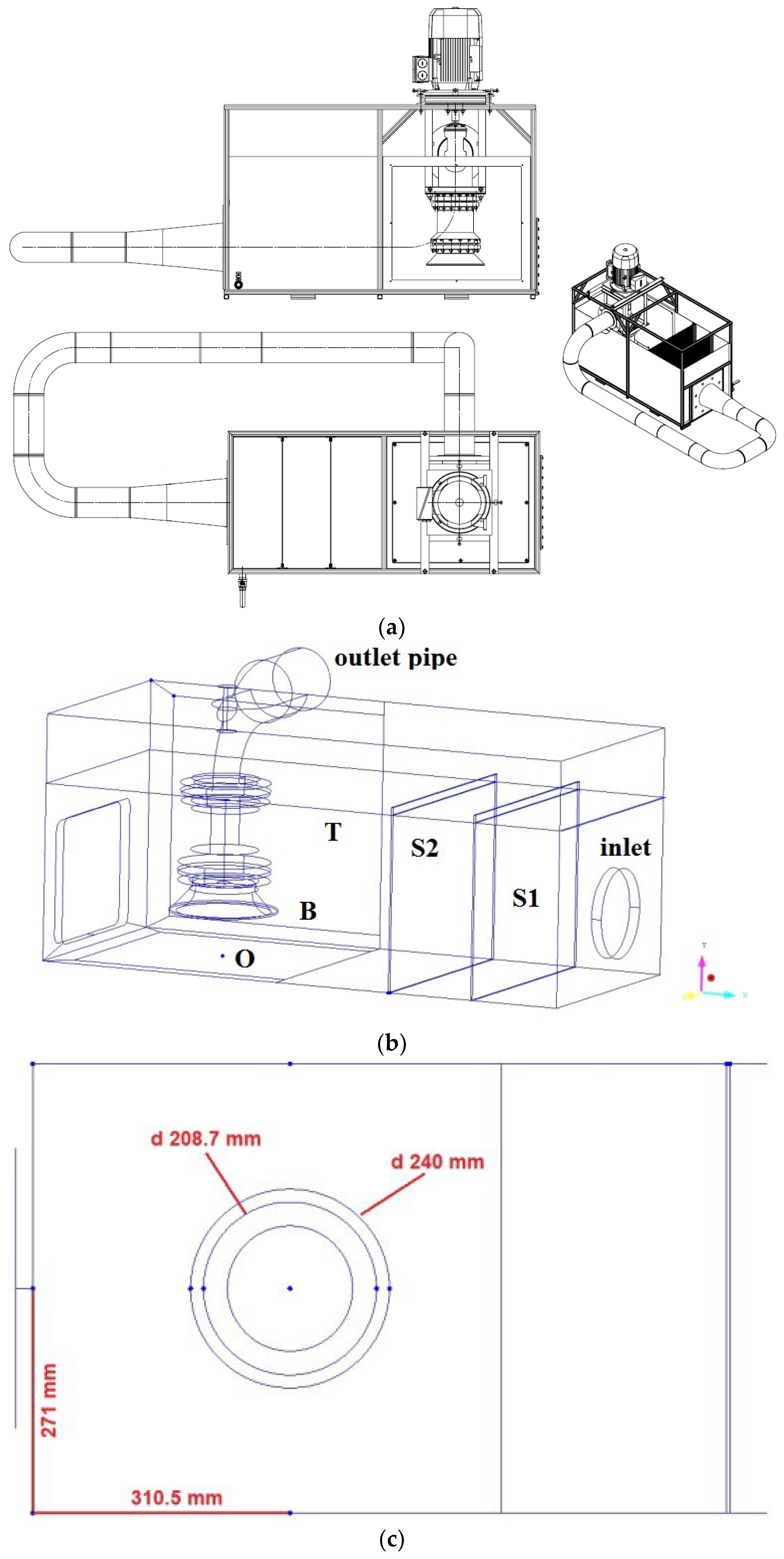
The experiments were carried out in the closed water circuit with a rectangular tank with the dimensions (L × W × H) 1272 × 542 × 550 mm3. The coordinate system is introduced so that the x-axis is oriented along the tank, the y-axis is identical to the pump axis of revolution/rotation and the z-axis is oriented according to the right-hand rule (Figure 1). The origin is placed on the bottom wall just below the impeller.
The water enters the tank by pipe from the right in the inlet, passing through two screens, S1 and S2, into the rectangular test section T. The water is sucked out from the tank by a suction bellmouth B and passes out to the outlet pipe. The coordinate system origin is labeled as O. Some key dimensions are shown in Figure 1c.
Both the front and the bottom sides are equipped with transparent windows, which enable lighting the space with a laser sheet and simultaneously recording the PIV images. The axial flow pump is located in the plane of symmetry and 310 mm from the left wall (see Figure 2).
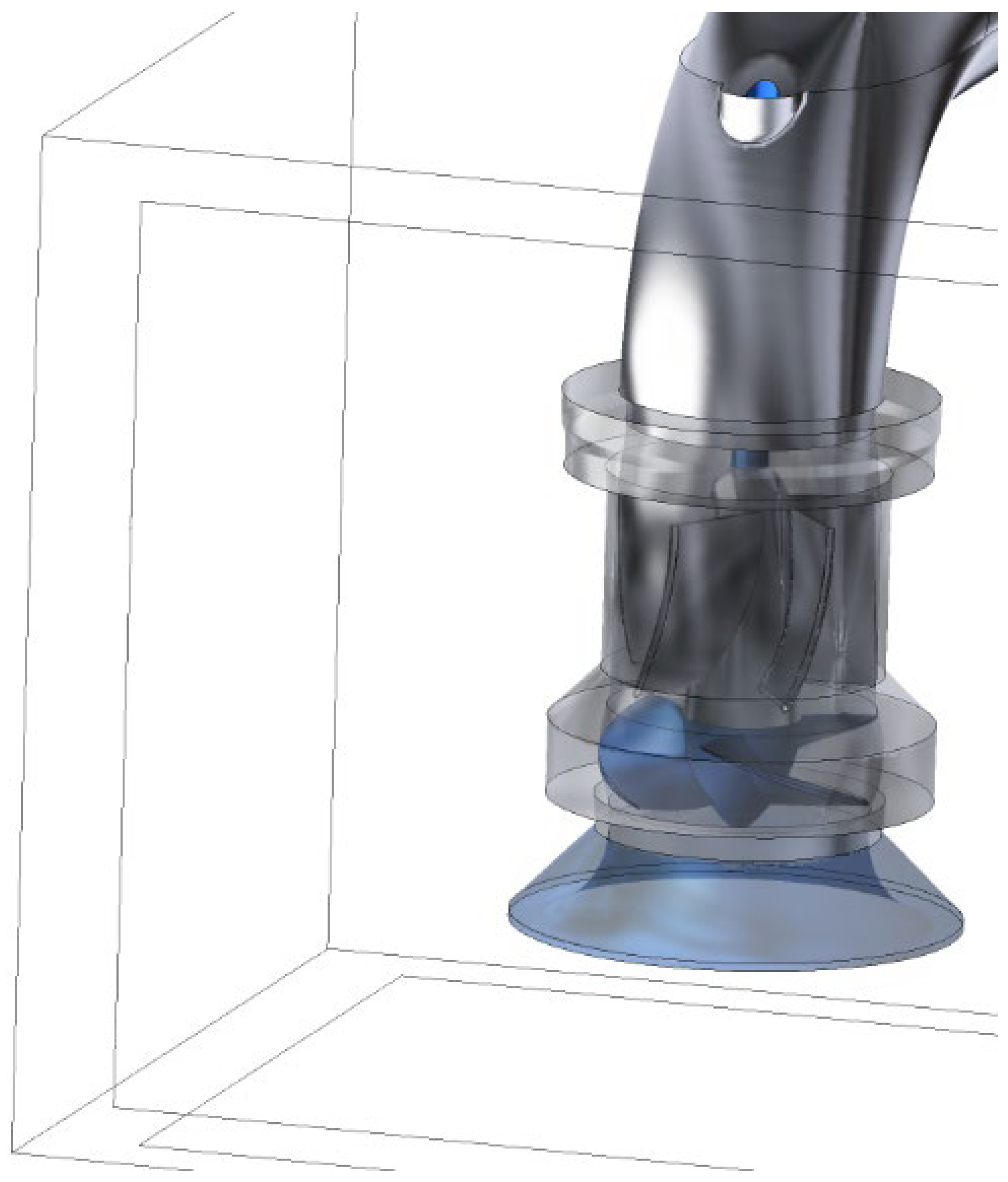
The impeller has three blades and is 150 mm in diameter (Figure 3).
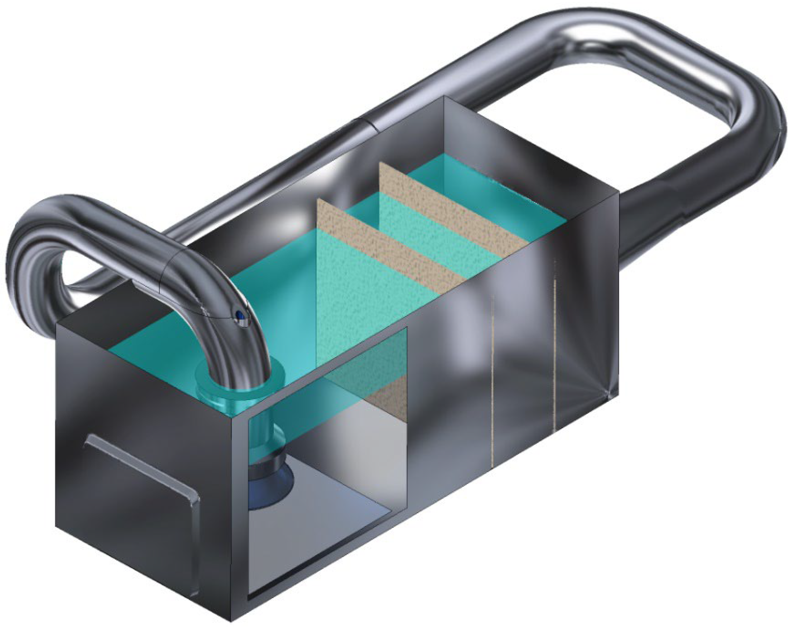
The impeller revolution was set to 1500 min−1 counter-clockwise. The lower edge of the suction bellmouth has a diameter of 240 mm and is placed 100 mm above the tank bottom. The water circulates from the pump outlet through the piping back to the tank, which enables the water to be filled easily with seeding particles. On the right-hand side of the tank, two screens are installed (200 and 400 mm from the right-hand wall). They help to create sufficiently uniform inlet flow with fine-grained homogeneous turbulence (Figure 4).
The screen mesh sizes are 10–12 and 5–8 mm, respectively. The flow rate during all experiments was set to the constant value of 52 L/s. The initial water level has been set to 398 mm above the tank bottom. The volume flow rate was measured with the induction flowmeter (accuracy 0.05 L/s), and the mean water level was controlled by the ultrasonic level transmitter (accuracy 1 mm).
Our experimental research included both the visualizations of unsteady flow phenomena with the high-speed camera and the PIV measurements in selected vertical and horizontal planes.
3. Visualizations
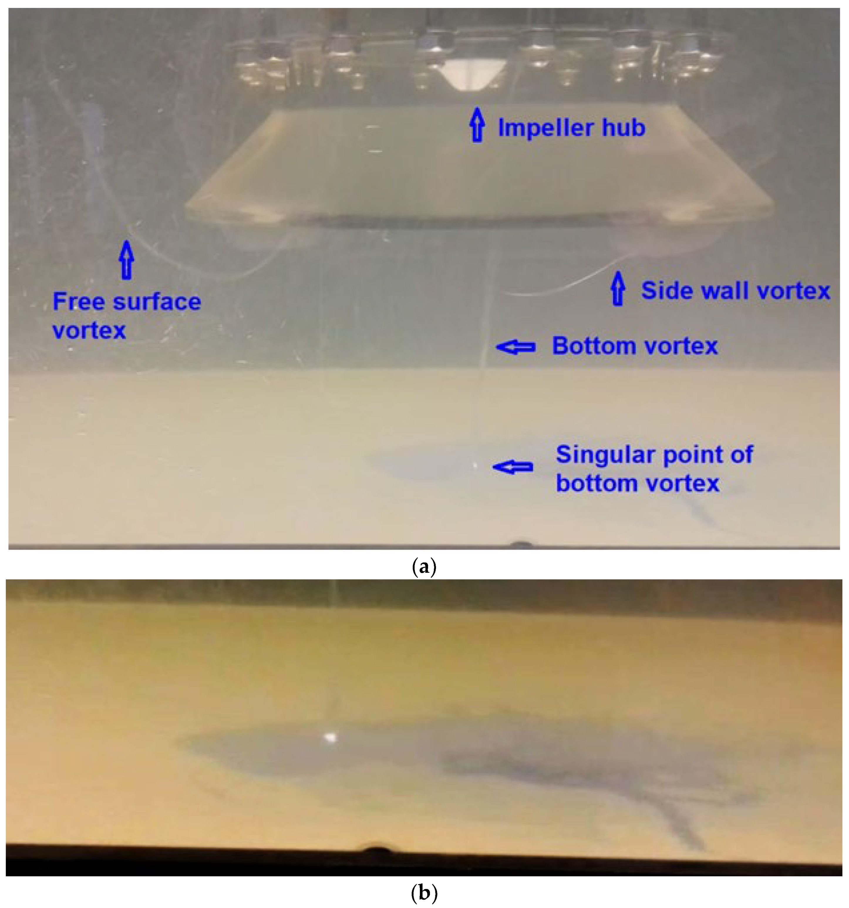
To enable better visualizations of flow phenomena with the high-speed camera, the water has been seeded with particles with a density only slightly higher than water density and illuminated with intensive dispersed light. The sedimentation time of particles was in the order of several hours. These particles followed the water flow and, when lightened, gave a simple picture of the velocity vector field. At the same time, particles already sedimented at the test section bottom enabled visualizing the position and movement of the singular point linked with the bottom vortex. Figure 5 shows three basic vortices below the pump suction bell. The bottom vortex, which is very stable (in the sense of permanent presence), can be easily identified because of the vapor trace in the vortex core. Only one bottom vortex has been identified between the bottom wall and the pump suction. It has been moving in the range of several centimeters from the pump axis of revolution, as can be seen in Figure 5. Its singular point moves on the bottom wall at a speed of several centimeters per second. Much less stable are the vortices rising on the side walls; they could be observed only part of the time. Only very rarely more than one side vortex could be identified at the same time. Different types of vortices could be found between the water level and the pump suction. Both the case with only one free-surface vortex and the case with two counter-rotating ones could be observed (Figure 6), though most of the time, only one vortex could be identified. Free-level vortices have been changing their character from the surface dimples up to the full air core ones.
4. Methods
The results of the application of both experimental methods and numerical simulations are to be presented. The numerical results were validated.
4.1. Experimental Techniques
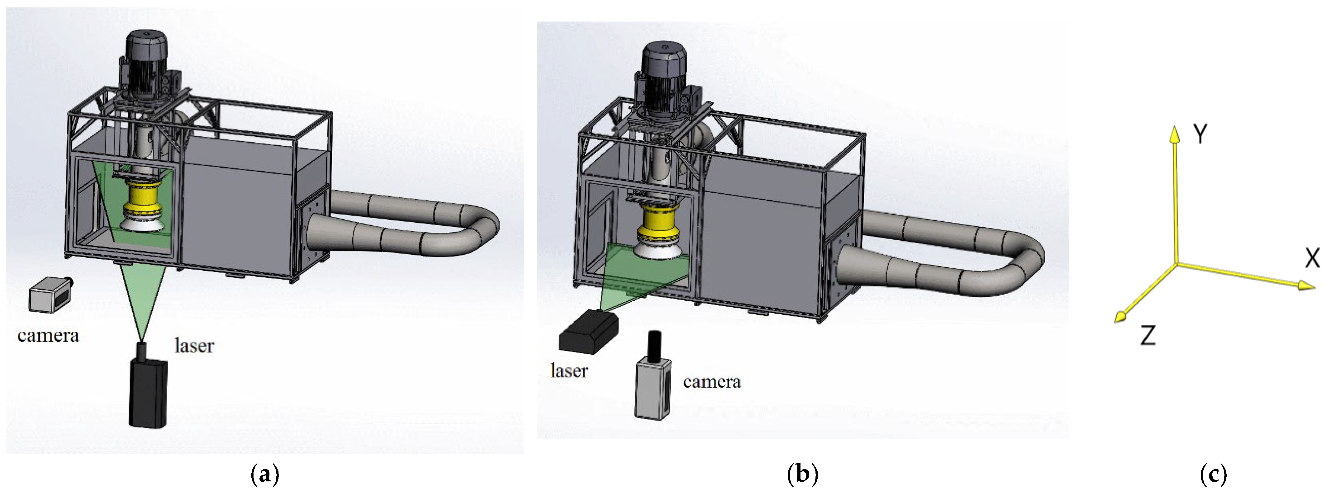
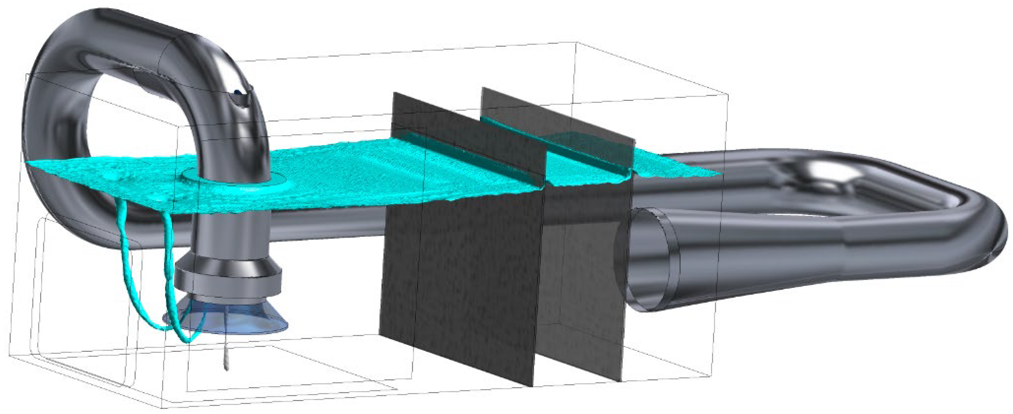
For the steady-state regimes and the vortex dynamics, the PIV measurements with one camera (see Figure 7) have been applied as in the case of siphon performance [8]. The PIV results are represented by distributions of the two components of velocity vectors in the plane of the laser sheet, shown in green in Figure 7. The measurement apparatus consisted of the CMOS camera and the laser by Dantec Company. The laser was New Wave Pegasus, Nd:YLF, double-head pulse type with the light wavelength of 527 nm, the maximal frequency is 10 kHz, the single-shot energy is 10 mJ (for 1 kHz). and the corresponding power is 10 W per one head. The camera Phantom V611, with a resolution of 1280 × 800 pixels, was able to acquire double snaps with a frequency of up to 3000 Hz (for full spatial resolution), and it used the internal memory of 8 GB for the data storage within a single experiment. Hollow glass spheres coated by silver layer HGS-10 were used as tracking particles. Their typical diameter was 10 microns, and they have a very similar density to water, so they can follow the flow very faithfully. The data have been acquired and post-processed using the Dynamic Studio, Matlab and Tecplot software tools. To get a very complex view of the flow structures, we utilized a combination of measurements in both vertical and horizontal planes. However, it is possible to combine only data processed by time-averaging. The vertical planes have been located in the positions z = 0, 70 and 130 mm, where z is the distance from the sump symmetry plane. Horizontal planes have been located at the distance of y = 50, 70, 105, 125, 155, 205, 255 and 305 mm above the bottom.
Calibration was performed in one vertical plane (z = 0 mm) and also for the horizontal plane at y = 50 mm. Horizontal measurements were performed below the impeller and also above it. The traversing system enabled the synchronized displacement of the laser and camera, which allowed the use of a single calibration for more parallel Planes of Measurements (PoMs). Both approaches resulted in dimensions of Field of View (FoV) equal to approx. 330 × 210 mm2. The adaptive correlation algorithm using Interrogation Area (IA) 32 × 32 pixels was utilized, resulting in 79 × 49 valid vectors in each PoM. Thus, the spatial resolution is about 4 mm.
Two acquisition strategies have been applied. For the time-averaged measurements, 1000 measurements with an acquisition frequency of 10 Hz have been acquired, representing 100 s. However, to study the dynamics of vortical structures, the data were acquired with a frequency of 100 Hz using 4000 snapshots covering 40 s in physical time. The accuracy of PIV velocity measurement is about 2% of the maximal velocity value within the PoM.
4.2. Numerical Simulations
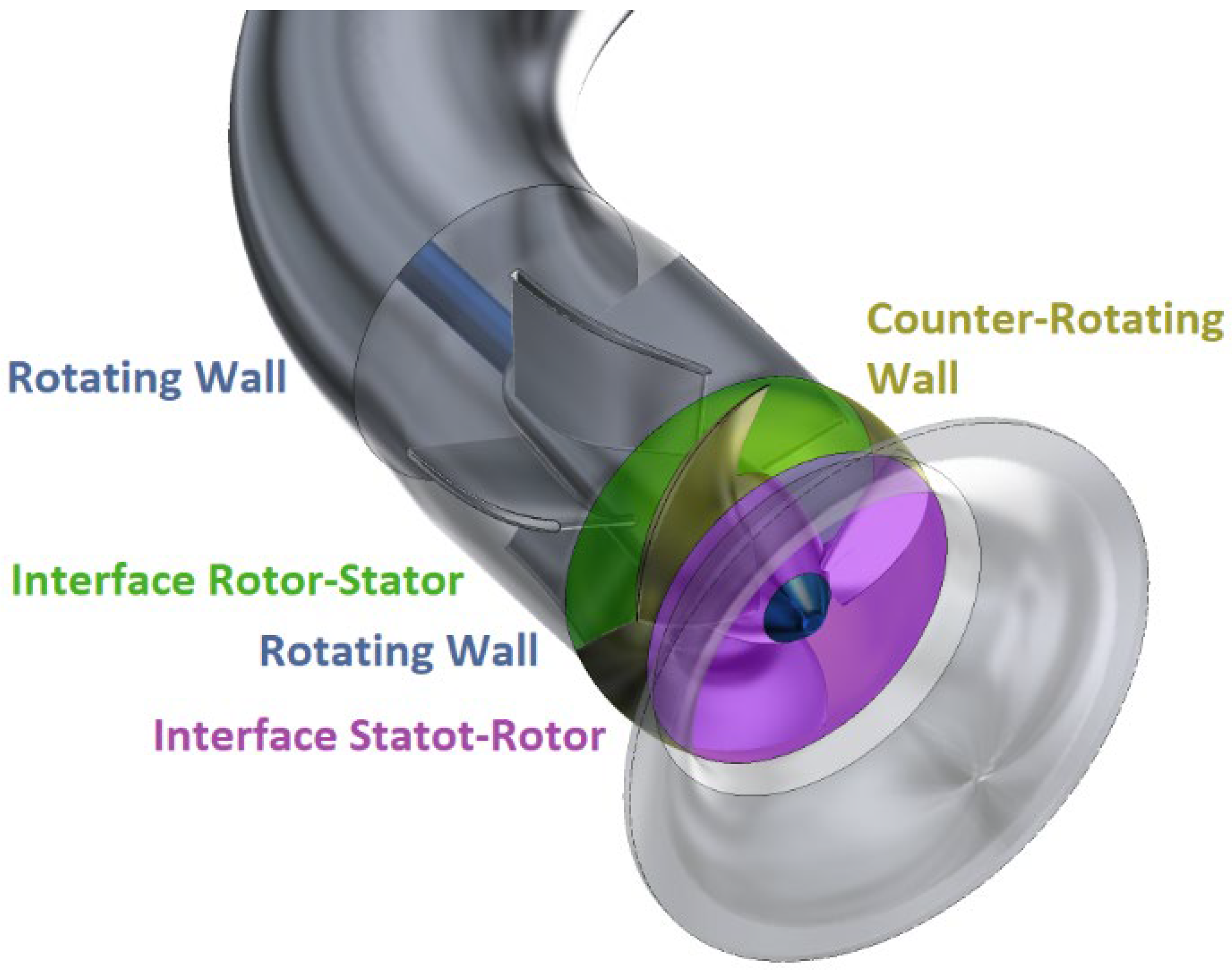
The CFD software ANSYS CFX release 19.2 [17] has been applied to solve the three-dimensional Unsteady Reynolds-Averaged Navier–Stokes (URANS) equation. Because of the rotating flow inside and under the pump, the experimental device misses any symmetry plane, and the computational domain (see Figure 2, Figure 3 and Figure 4) must represent the full three-dimensional suction object, including all pump components and piping. Moreover, full unsteady interactions between the pump impeller and the stationary parts are kept with the time step representing two degrees of pump impeller revolution. The subdomain of the pump impeller is rotating with a prescribed rotational speed. All the other subdomains inside the pump, rectangular test section and piping, are stationary. There are two interfaces between the stationary and rotating subdomains, as can be seen in Figure 8. Because the impeller nut and the shaft are rotating in the stationary subdomains, their surfaces are treated as rotating walls. On the other hand, the impeller shroud, which is, in fact, stationary, has to be treated as the counter-rotating wall. All the hydraulic surfaces are considered to be smooth, without prescribed roughness. As the computational domain represents a closed loop, there are no inlet and outlet boundaries and the mass flow is generated by the impeller rotation and controlled by the pressure losses in the computational domain, including screens. The screens have been described as porous layers with the permeability derived from the numerical tests with small (100 × 100 mm2) parts of the screens modeled in full detail. This strategy has been adopted to keep a reasonable size for the computational grids. The computed mass flow rate has been compared with the mass flow rate measured during the experiments; the detected differences were a few percent. Concerning the boundary condition on the top of the rectangular test section, the opening boundary has been used to enable the air to flow both inside and outside the computational domain.
All simulations are based on constant property fluids. It means that the water, water vapor and air are considered as incompressible fluids with constant densities and constant temperature. The free surface flow, including the gravity effects, is based on the Volume of Fluid (VOF) method evaluating the volume fraction of each fluid. A non-homogeneous model of multiphase flow has been applied with different velocities for the water, vapor and air fractions [17]. The Zwart cavitation model [18] has been employed to describe the interphase mass transfer during the cavitation effects. To capture all possible factors acting on the free surface vortices, the Coriolis forces resulting from the earth rotation have been added into the computational model, though they are much less important than the geometry and other physical factors [19].
The structured computational grids have been used inside the rotating and stationary parts of the pump, pipes and screens. To keep the grid inside the tank sufficiently isotropic with acceptable values of y+ monitored in time (close to 1 on the majority of solid surfaces), the unstructured computational grid with prismatic elements inside the boundary layers has been applied. The overall number of computational grid points is approximately 17 million. The maximum distance of the neighboring grid points in the tank is about 3.3 mm, which enables relatively thin vortices to be captured. As it will be described in the next chapter, the calculated vortices have been very unstable, with the random nature of their appearance and topology. For that reason, it has not been possible to provide a standard grid independence test in which the results could be compared and verified directly by the experimental data. Consequently, the computational grids (especially inside the rectangular tank) have been tested and optimized in several steps to keep acceptable values of y+ and to capture sufficiently small flow structures. The resulting computational grid represents a reasonable compromise between these requirements and the possibility of using a 16-core-based workstation with 128 GB of memory.
The initial calculations employed the URANS equations with the standard SST turbulence model and then switched to the SAS scale resolving simulations ([20,21]), which are more suitable for predicting small vortical structures. The high-resolution scheme of the second order has been used for the momentum equations, and the first-order scheme has been used for the turbulence modeling. The time discretization is based on the second-order backward Euler scheme.
5. Results
Now, the results are to be presented in terms of vortices description using both experiments and CFD.
5.1. Surface Vortices
The surface vortices were found to be very unstable. They were studied by visualizations (see Section 3) and partly using CFD.
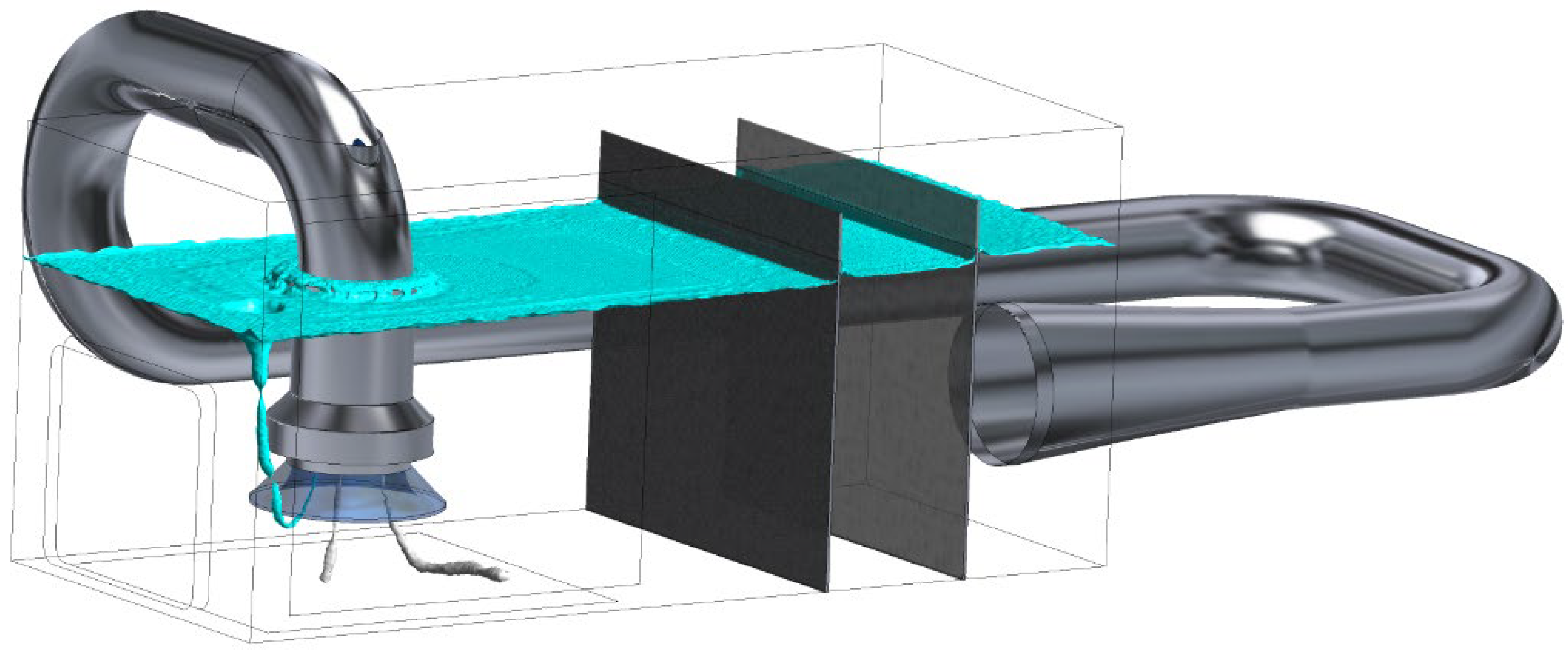
Similar to the visualizations, the CFD simulations also show that the only vortex that is stable and present permanently is the bottom vortex, which moves around the pump axis revolution. Further, one side vortex and one or two free-surface vortices have been kept with the simulations. Unfortunately, they have been very unstable, and the computational capacities do not allow any rule on their formation or frequency analysis to be found. Figure 9 and Figure 10 show a complex system of vortices in the testing tank, including the bottom vortex, one free-surface vortex and one side-wall vortex. The iso-surfaces of constant air volume fraction of 5% (in cyan) and constant vapor volume fraction of 5% (in grey) have been used to visualize the vortex cores in Figure 9. The Q criterion has been applied in Figure 10. A pair of counter-rotating free-surface vortices can be seen in Figure 11, together with the bottom vortex.
5.2. Bottom Vortex
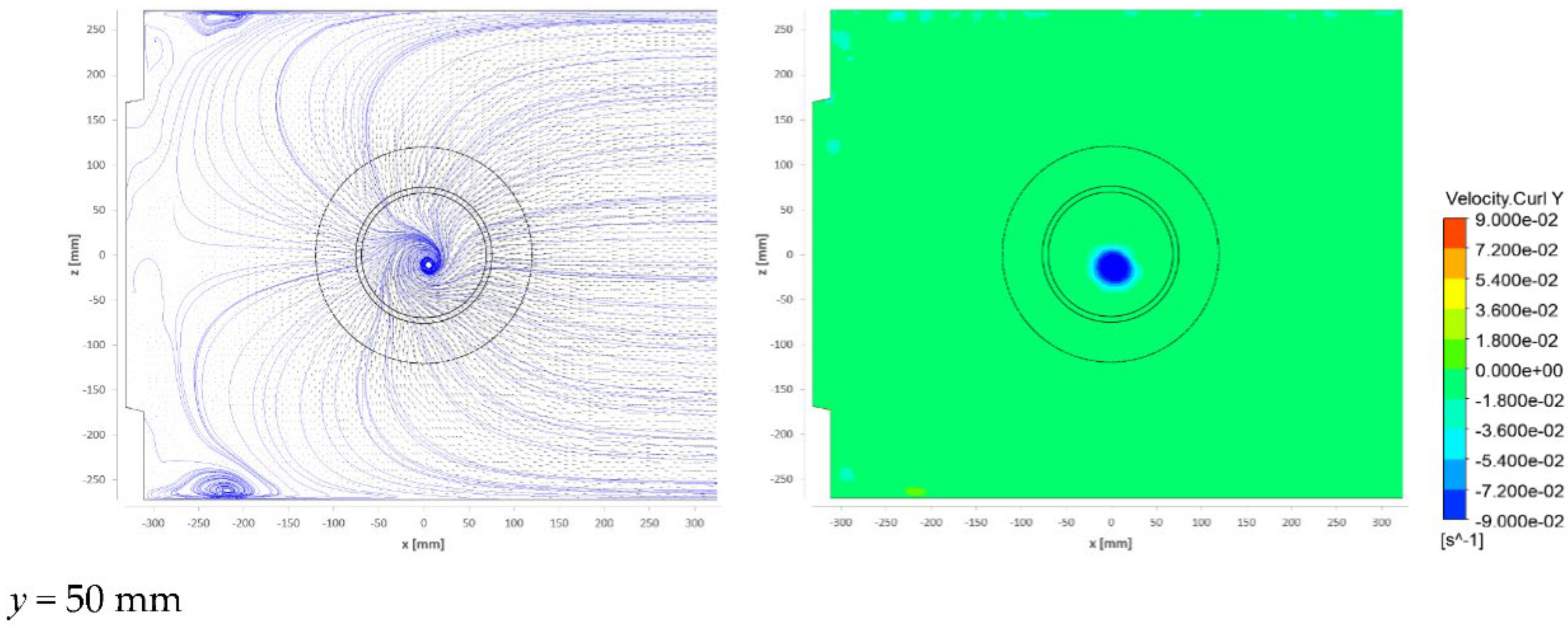
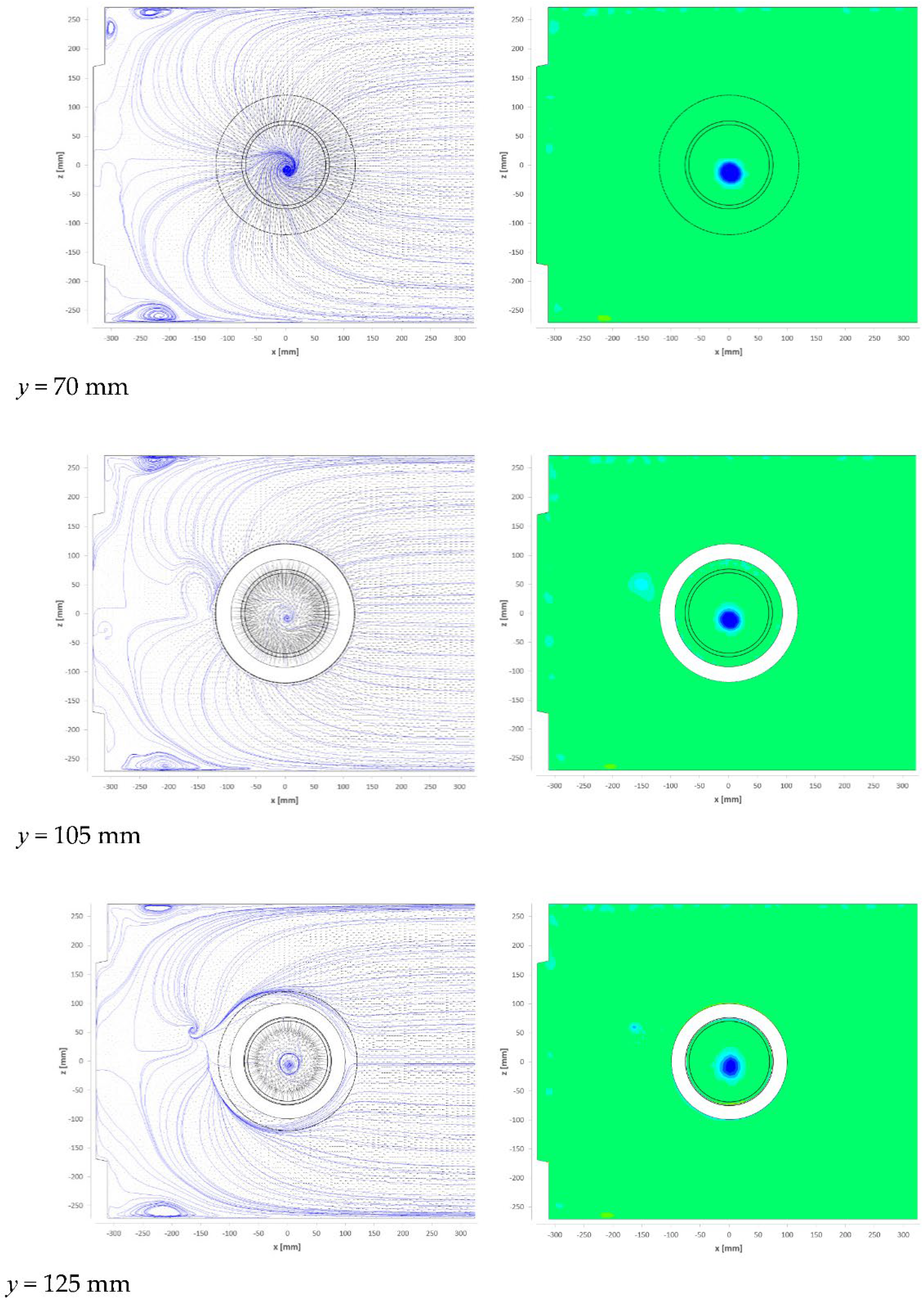
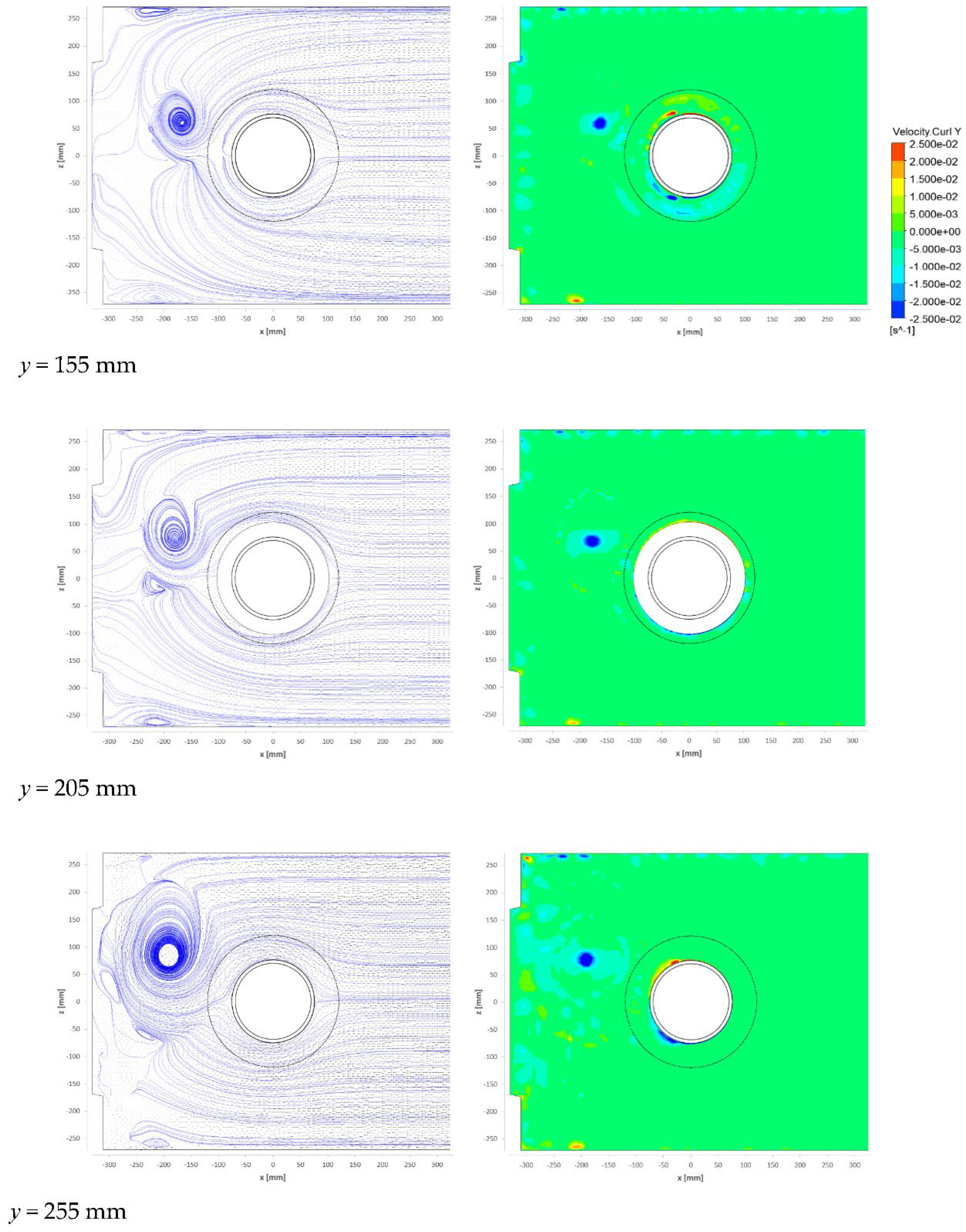
Because of the unsteady character of flow structures, which have been changing their position as well as the topology, it has been a little bit problematic to present time-averaged results of the numerical simulations. That is why the simulations have been averaged just for a short time when the topology and position of the vortices remained similar (time scale of order 10−1 s). Figure 12 and Figure 13 show the position and character of the bottom vortex and one single free-surface vortex in the horizontal planes spaced from 50 to 255 mm from the tank bottom. Both the vector lines and vorticity distributions are shown for every plane. The general term “vector lines” is used in the description of results as “streamlines” are defined as “vector lines of the instantaneous velocity fields in 3D”, which is not the case for the time-averaged velocity fields in 2D.
In section y = 50–105 mm, the bottom vortex could be identified with its center close to the coordinate system origin. For the planes y = 125 mm and above, the surface vortex located near position [−200;70 mm] could be detected.
5.3. Intake Flow
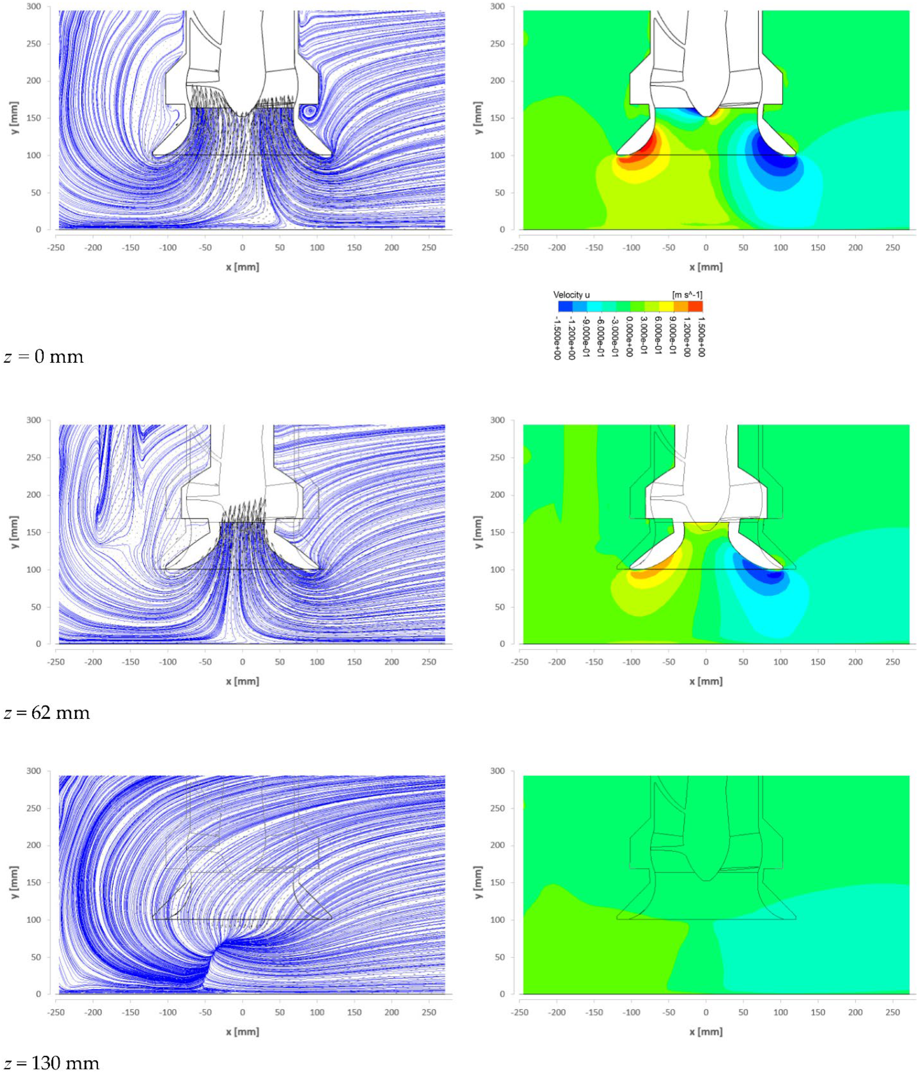
Figure 14 shows the vector lines and longitudinal velocity distribution in vertical planes z = 0, 62 and 130 mm. Here the vector lines and x-velocity component distributions are shown. The bellmouth section by the projection plane is white, while the object silhouette is shown in black lines.
It can be seen in the vertical plane z = 62 mm that the flow is influenced by the free-surface vortex situated left of the bellmouth.
The numerical simulation shows a good agreement of the basic behavior of the flow phenomena close to the pump suction. Specifically, the bottom vortex is captured in a very good way. The comparison of free vortices obtained by the experiments and by the CFD tools is much more difficult, as these phenomena are highly unsteady and unstable. Their description depends on the way of time averaging, but the most important factor is the fact that during the experimental research, every horizontal or vertical plane is captured in a different instant.
The inflow into the bellmouth from both sides of the x-direction could be detected from the pictures in Figure 14.
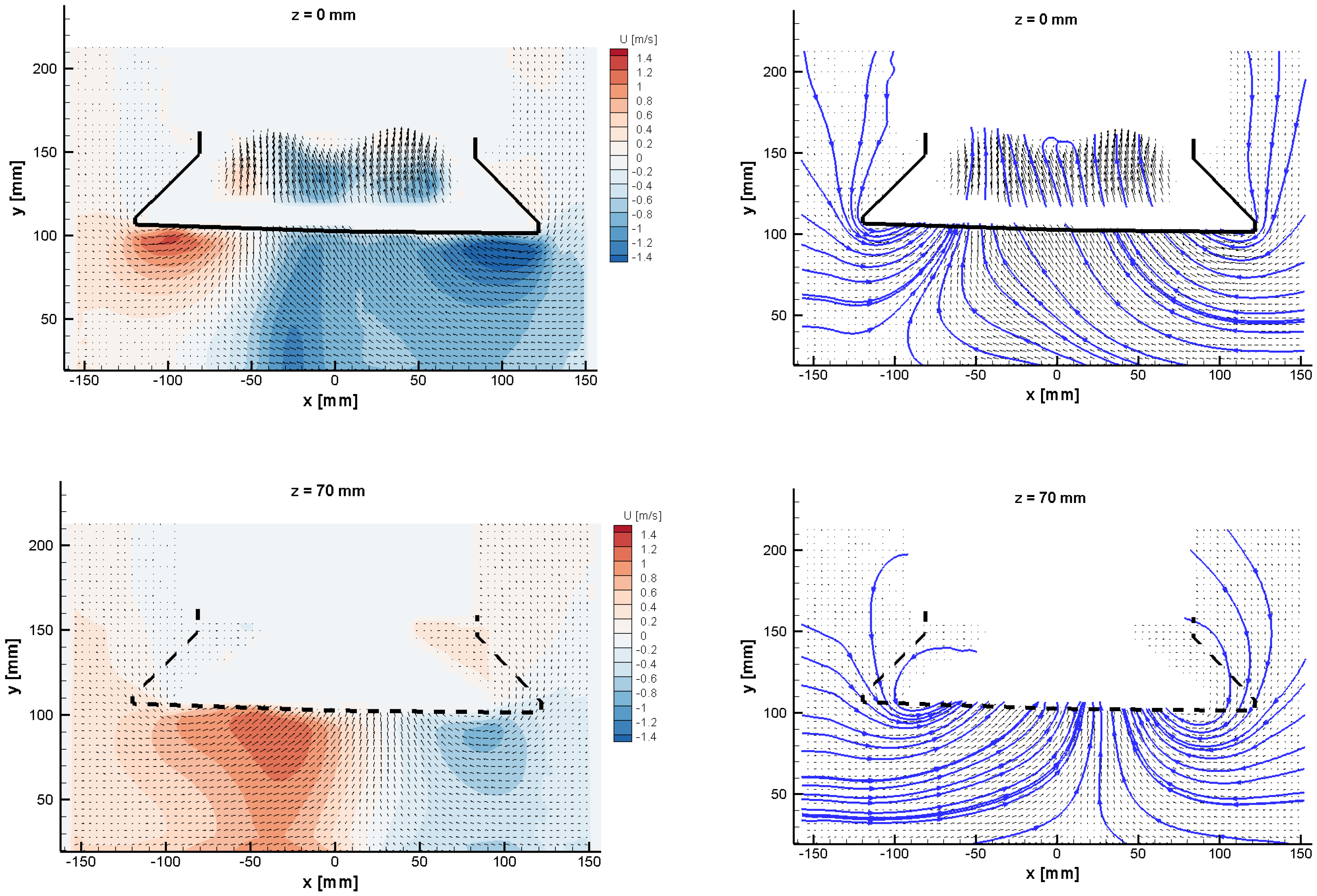
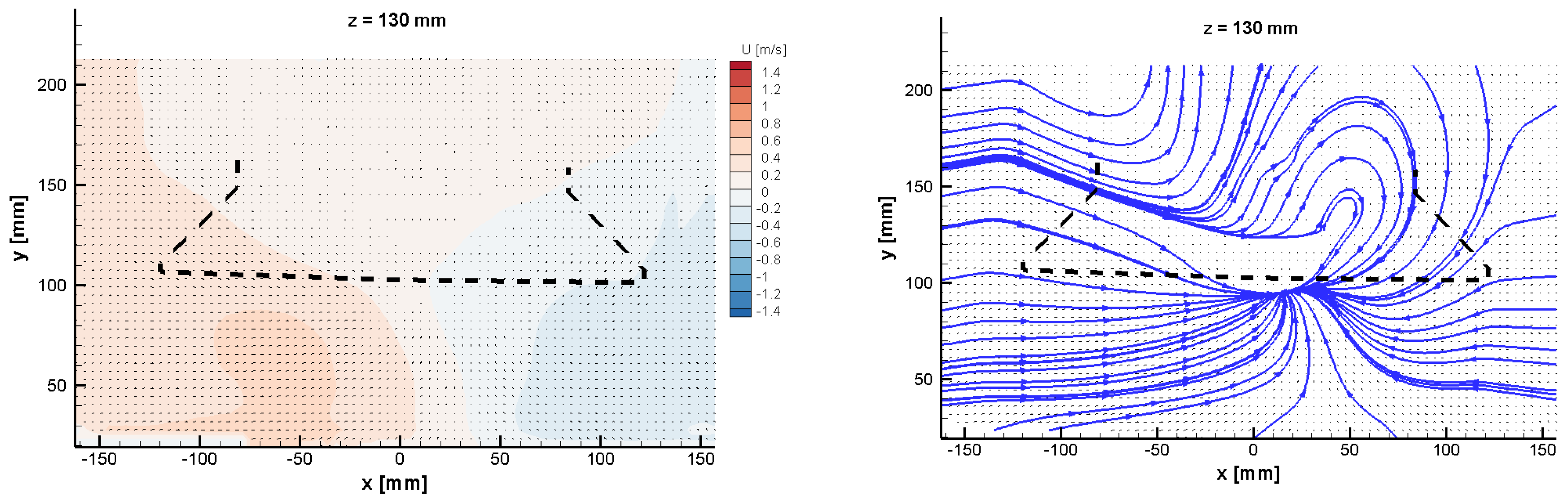
The experimental results and velocity fields in vertical planes z = 0, 70 and 130 mm are shown in Figure 15. The flow enters the sump volume from the right-hand side. The black vectors represent in-plane velocity components, and the color is a scalar value (horizontal velocity component); vector lines are added in blue color. The velocity distributions in the vicinity of the bellmouth show very good agreement with CFD data, especially for planar data acquired in the plane of symmetry (z = 0). The vector lines below the suction pipe do not rise up as vertically in comparison with the calculated results. The other two PoMs reveal the flow topology closer to the side wall of the sump. The flow is attracted from above, and the flow is bent 180° in the vicinity of the bellmouth edges. The singular point (zero in-plane velocity) is situated 20 mm to the right of the center. The solid black line indicates the cross-section of the bell. The dashed line is its projection in the other PoM. Note, the bellmouth is not perfectly oriented perpendicularly with the bottom wall in Figure 15 as the physical model was inserted with a small deviation, and so the camera was slightly tilted.
The experimental results in Figure 15 show a not-so-regular input flow as the CFD in Figure 14. While the velocity distribution in the plane of symmetry z = 0 is deflected towards the left-hand side, in the position z = 70 mm, the situation is opposite for the experiment. The inflow in the case of CFD for both z = 0 and 62 mm is more or less symmetrical; compare Figure 14 and Figure 15.
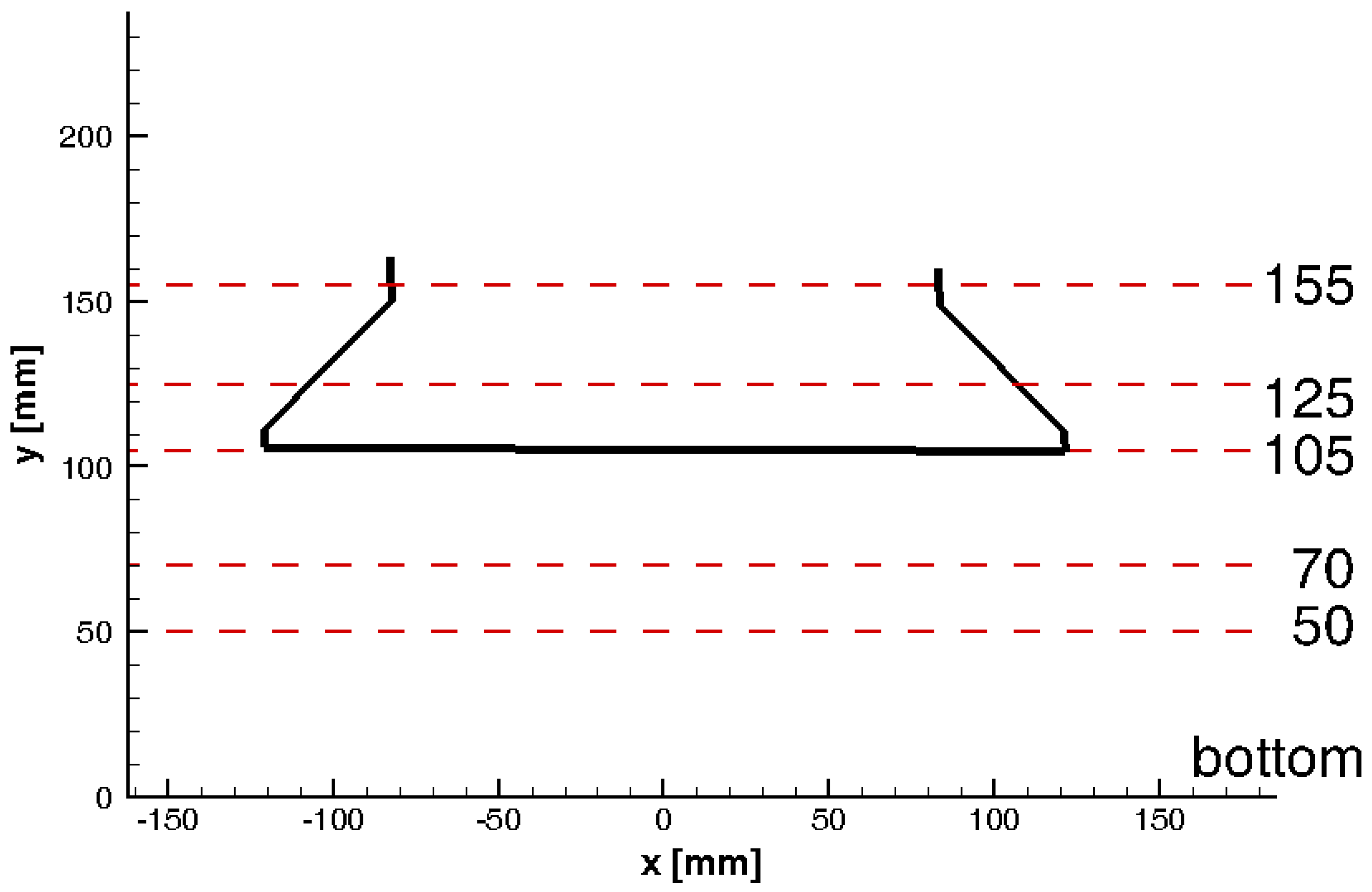
Further, horizontal planes will be introduced. In Figure 16, the positions of various PoMs are plotted to illustrate the flow under and above the bell edge.
There is an intersection of the bottom vortex at y = 50 mm, shown in Figure 17. The mean bottom vortex core position is situated close to the coordinate system origin in the geometrical center. The sense of rotation corresponds to the impeller revolution. The flow is entering the pipeline in a helix topology from distant surroundings.
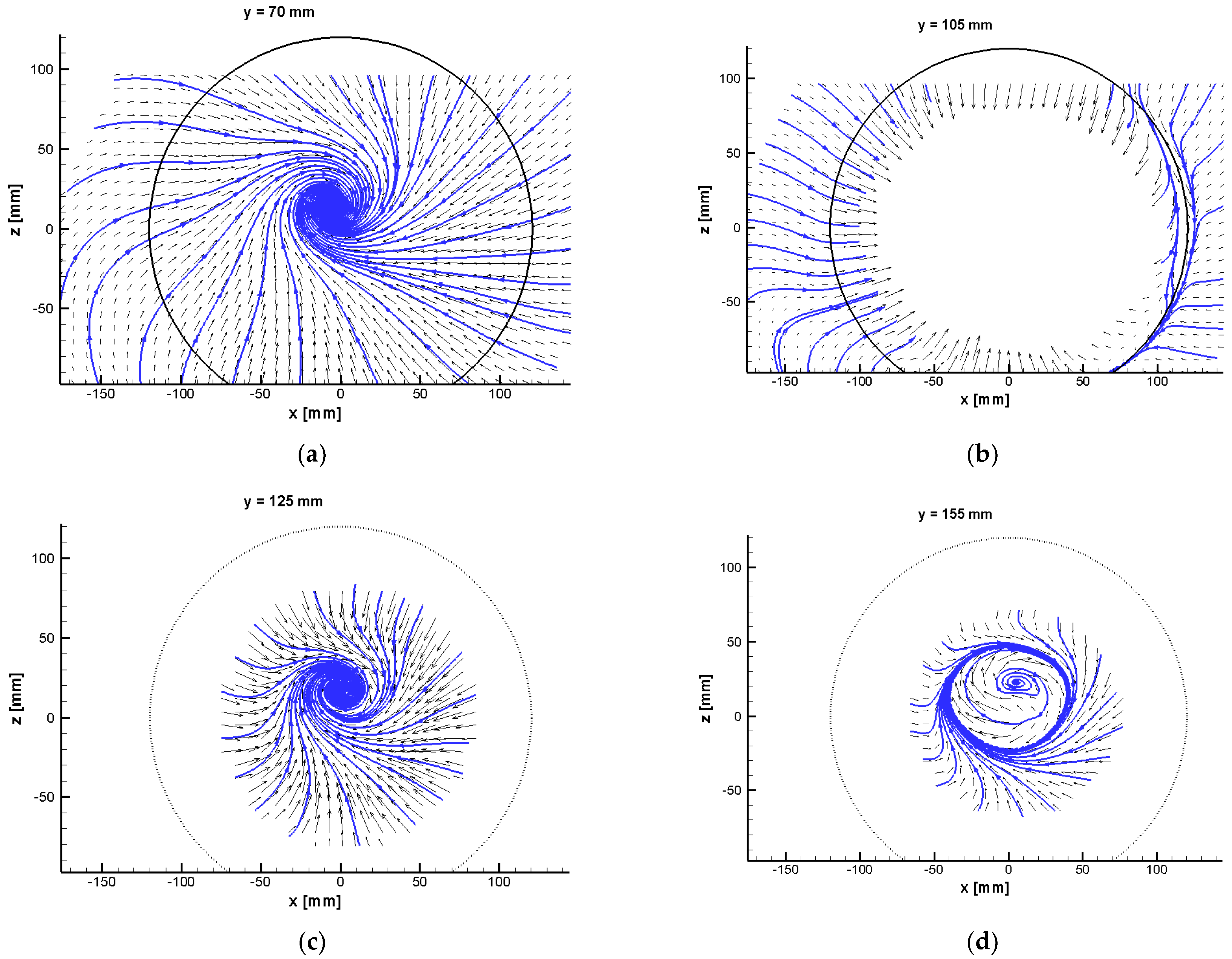
The bottom vortex topology is developing along the y-axis towards the impeller, as it is illustrated in Figure 18. The position of the vortex core does not change very much in the y-direction; however, in position y = 105 mm, the inner flow was not resolved because of laser light scatter on the bell edge.
The behavior of the free surface vortex is much more chaotic. This vortex can be observed on the left-hand side from the pipe inlet. The topology is developing according to Figure 19. Its center for time-averaged data is reaching the inner corner of the sump as the vortex approaches the water surface. The vortex is even out of PoM for y = 305 mm. Nevertheless, its averaged position agrees very well with the computed flow field.
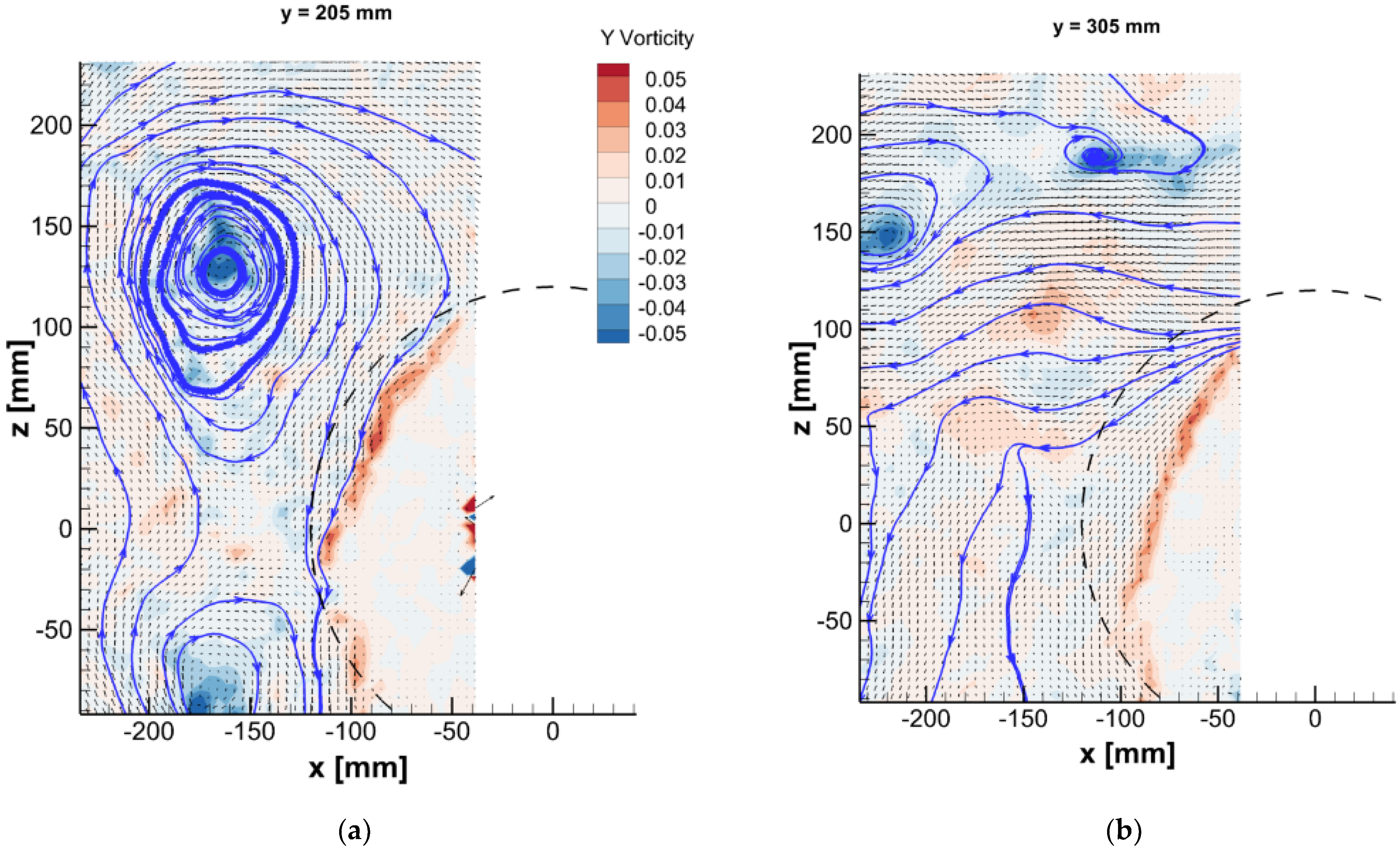
However, the surface vortex behavior is very dynamic with random elements. To demonstrate this fact, the two examples of instantaneous velocity fields in positions y = 205 and 305 mm are shown in Figure 20.
There are two instantaneous snapshots of the surface vortex for 205 and 305 mm above the bottom in Figure 20. The left-hand side of this plot reveals standard flow topology, which is changing its position and strength over time (see the next chapter). There is also rarely a situation when two vortices can be observed (this time is a pair with the same orientation).
5.4. Vortex Dynamics
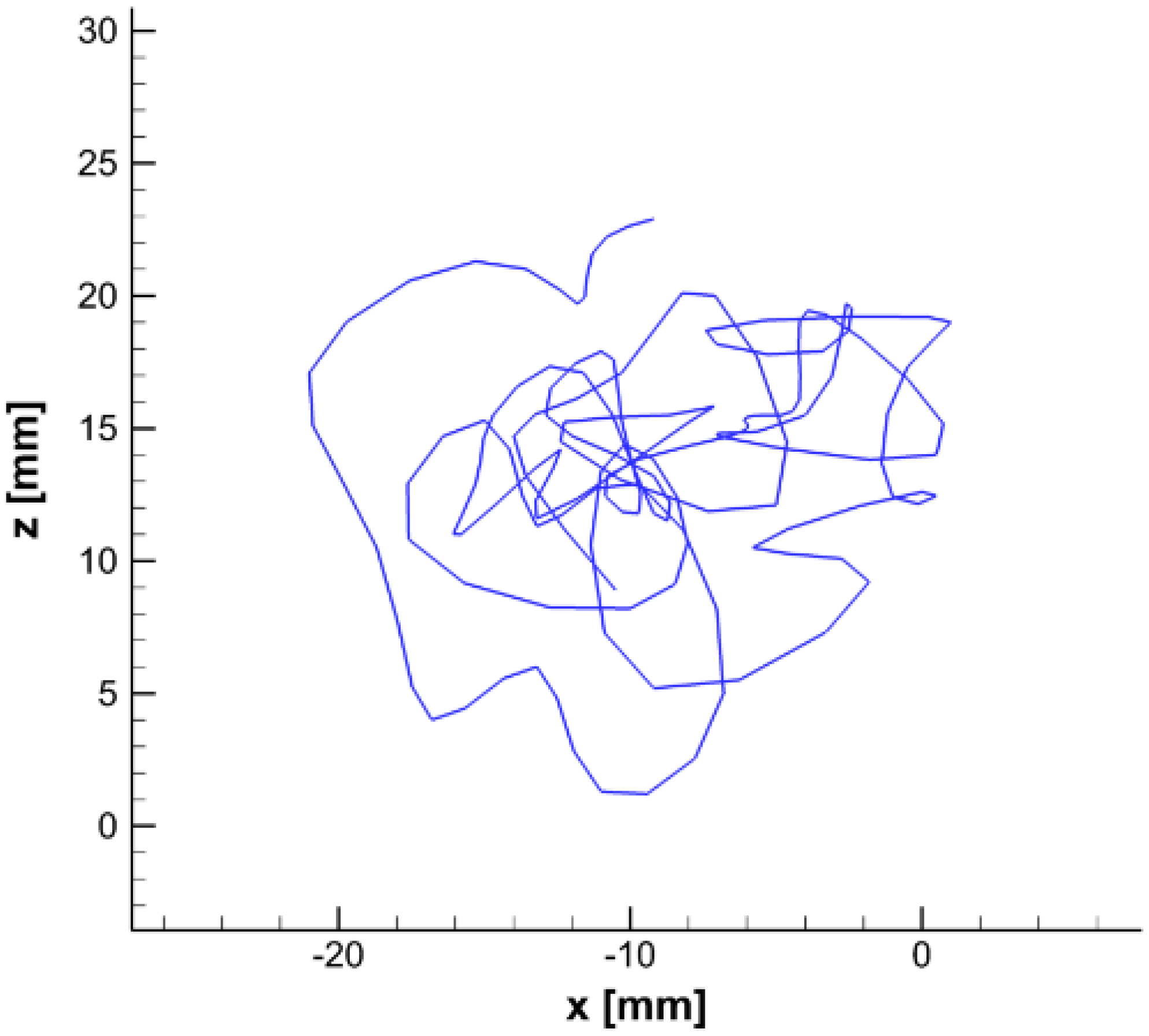
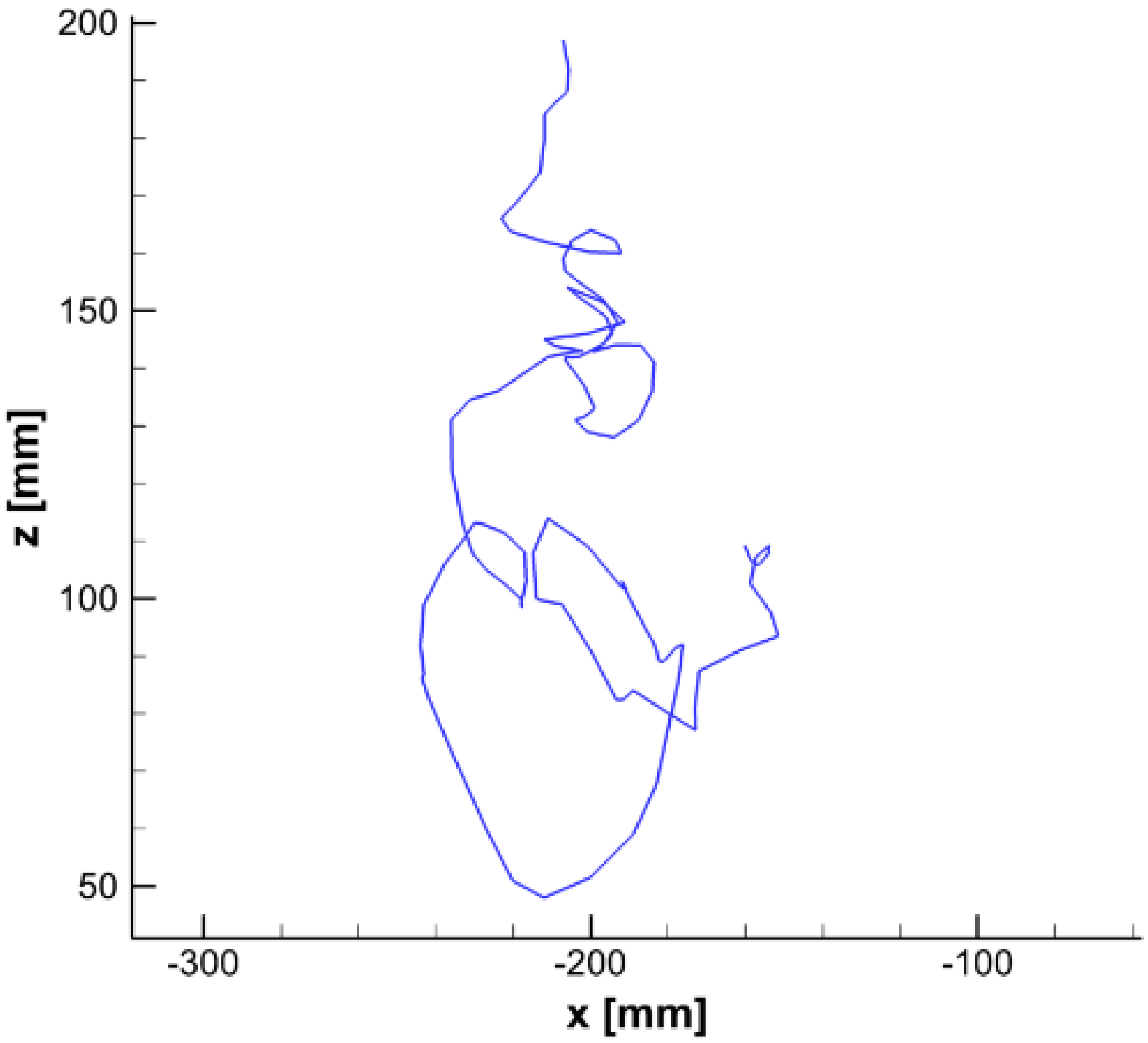
It was found that both the bottom vortex and the free surface vortices behave dynamically with no distinct periodicity in motion. It was proven that the vortex path is quite chaotic, although the vortex position was always detected inside some circle area. With a few exceptions, the bottom vortex occurs in the second quadrant. The precise position was determined from PIV images via image processing, the vortex core path for the horizontal plane y = 50 mm is given in Figure 21 for the time interval 6 s. The bottom vortex core motion is limited by the zone of the size of approximately 20 mm in the x and z-directions. The approximate speed of the core motion was detected up to 10 cm/s.
The first POD mode is shown in Figure 22 as an example. It is formed by a pair of counter-rotating vortices. This mode contains about 16% kinetic energy. Other higher POD modes consist of more vortices.
The behavior of the free-surface vortex was studied at plane y = 205 mm. The path of its core was also observed using PIV images. The free-surface vortex core was moving inside the area with a size of more than 100 mm, and the core velocity was about 30 cm/s, i.e., three times higher than the velocity of the bottom vortex, see Figure 23.
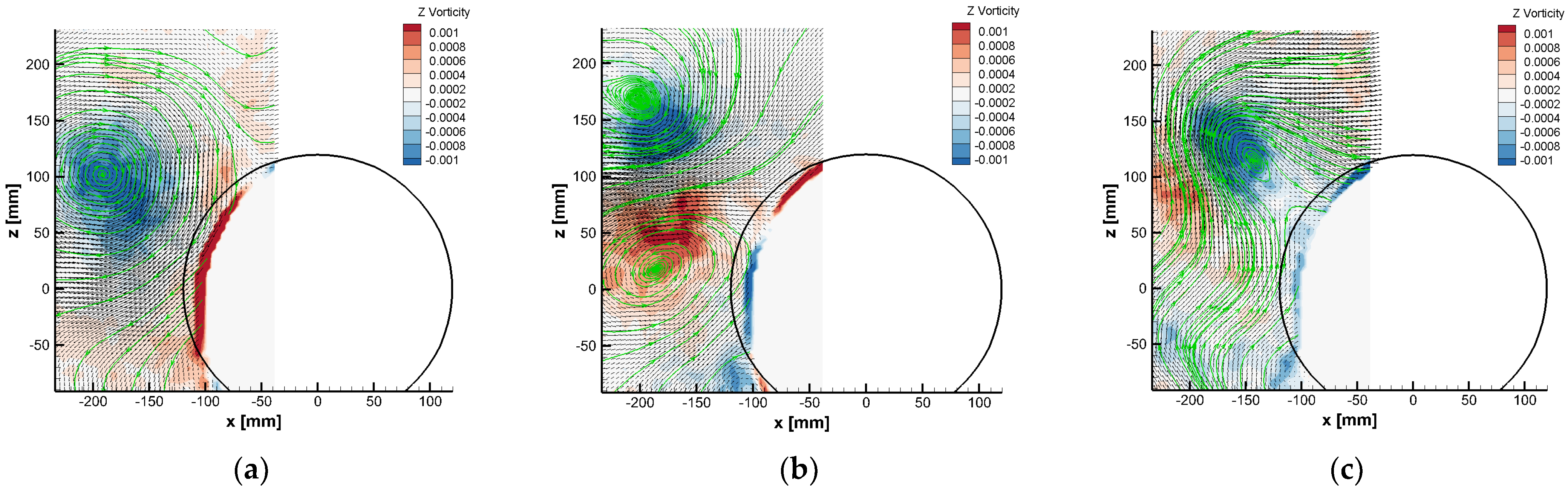
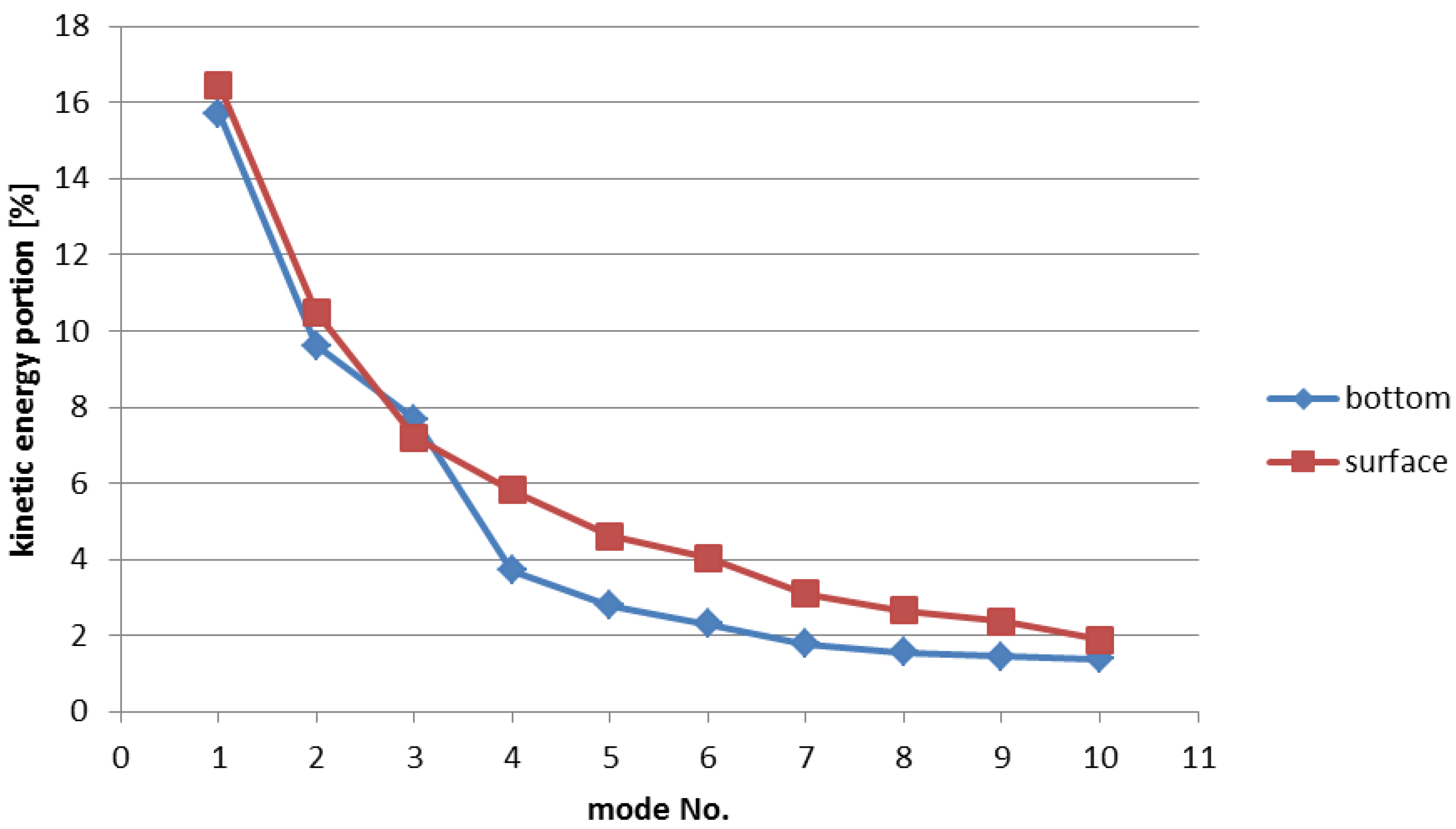
The POD method has been applied to the time-resolved data. Figure 24 reveals the three POD modes for this plane. First, the mode topology can be described as a single vortical structure occupying the space of the time-averaged vortex. The second POD mode consists of two vortices with opposite orientations, while the third mode topology is formed by a single vortex of negative vorticity with strong shear. The content of kinetic energy of the first 10 modes is given in Figure 25.
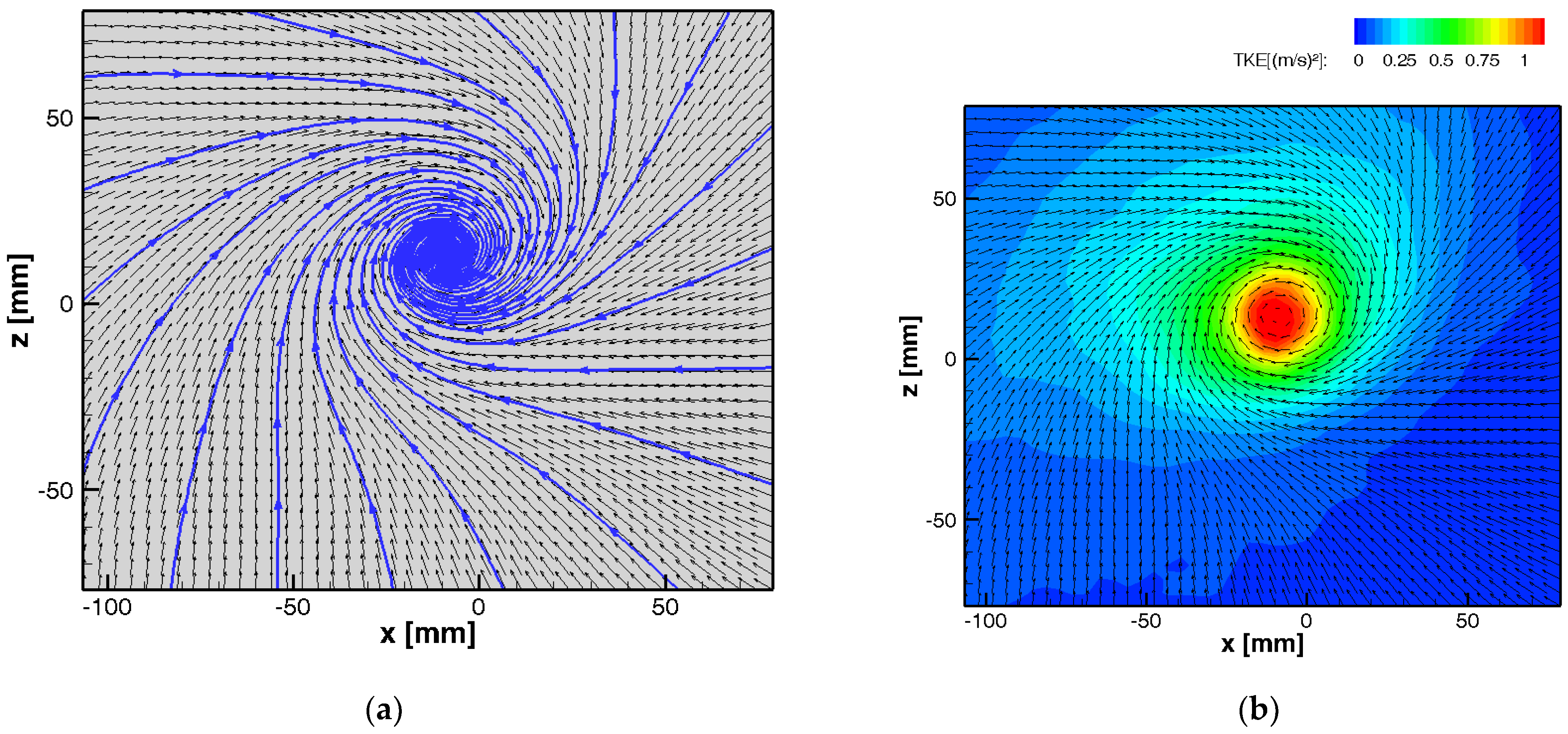
The dynamics of the bottom vortex have been studied on the horizontal plane at the position y = 70 mm in more detail. In Figure 26, there are the mean velocity field and Turbulent Kinetic Energy (TKE) distributions from the PIV measurement.
The Oscillation Pattern Decomposition (OPD) analysis has been applied to the velocity field time-resolved data acquired with a frequency of 100 Hz, and 1000 snapshots. The analysis results in OPD modes representing cyclostationary components of the topology dynamics with statistically limited time of life. Each OPD mode is defined by its topology, real and imaginary parts, frequency and mean lifetime. More information on the OPD method and results interpretation can be found in [16].
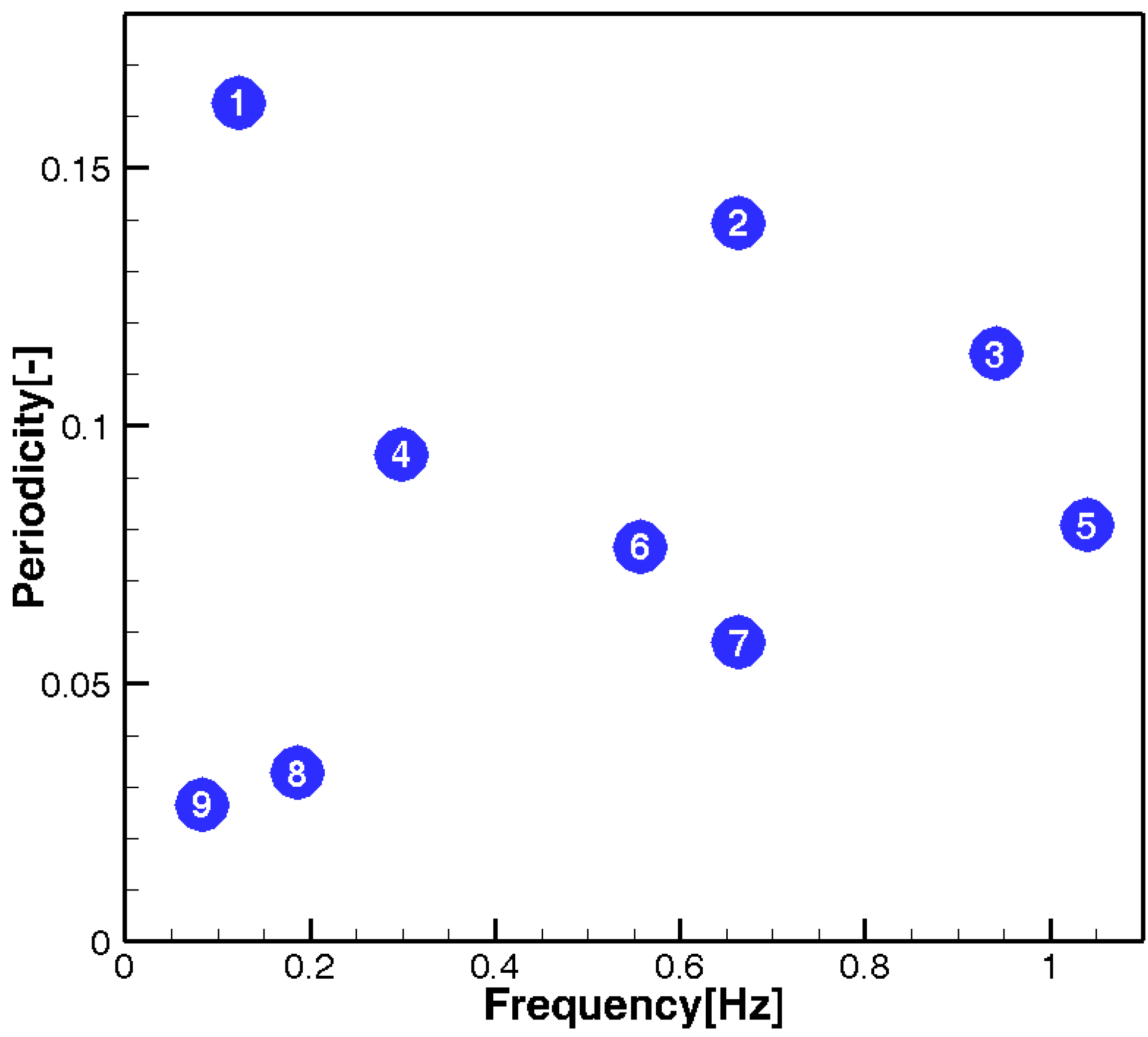
In Figure 27, there is the OPD spectrum shown, representing the nine most important cyclostationary modes in the plane defined by the frequency and periodicity. The frequency is the typical frequency of pseudo-periodical behavior, while periodicity is the lifetime expressed in multiples of the mode period.
The OPD mode’s importance could be quantified by the periodicity value; the higher periodicity, the higher importance. However, even in OPD mode 1, the highest periodicity value is about 0.163; this means that the mode appears randomly and disappears very quickly. The frequency of the first mode is about 0.124 Hz, the real and imaginary topologies are in Figure 28. The mode is represented by the counter-rotating vortex pair rotating around the common center. The color represents vorticity, positive in red and negative in blue.
In Figure 29, some higher-order OPD modes topologies are shown; the real parts only. The topology shows a combination of positive and negative vorticity concentrations; the most complex is OPD mode 5, with the highest frequency of 1.040 Hz.
The higher modes consist of several vortices of positive and negative orientations rotating in the plane.
5.5. Validation
The validation of the numerical simulations is performed with the help of flow in the neighborhood of the bellmouth intake. The flow topology is governed by the central vortex touching the bed just below the intake. The vortex is driven by the rotating pump rotor and is characterized by strong axial movement into the intake pipe. The vortex parameters were evaluated on the horizontal plane y = 50 mm above the bottom. The (x,z) coordinate system has its origin on the pump axis.
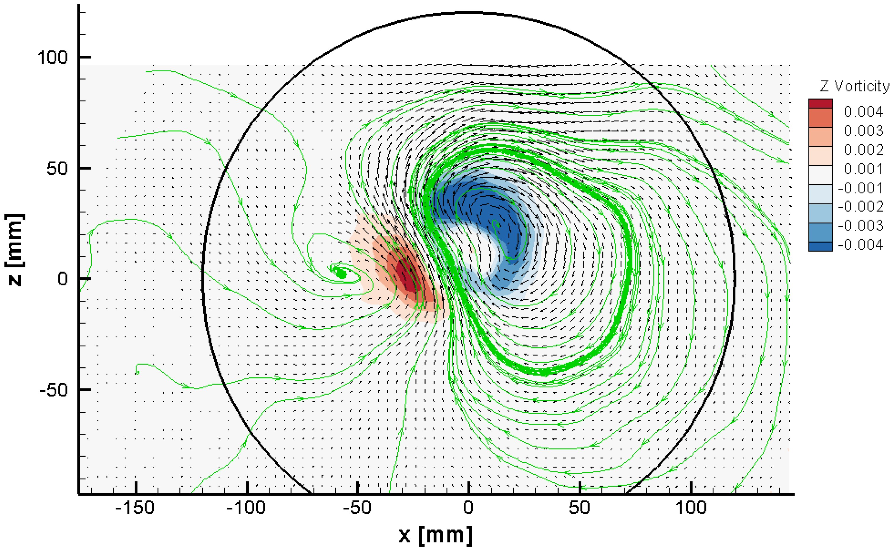
The topology of the vortex is shown in Figure 30; on the left, the result of the PIV measurement, and the CFD result is on the right. The result is shown in the form of mean velocity vector field, and the vector lines are added for better clarity.
The topologies of the PIV result and the CFD are not exactly the same. The vortex center was detected using the vector lines topology in the spiral focus. The position of the vortex center was detected [−0.0094;+0.0137] m for the PIV data and [+0.0053;−0.0106] m for the CFD data. They are denoted by the cross. The vorticity is concentrated close to the vortex center. The vorticity y-component ω was evaluated:
The vorticity distributions are shown in Figure 31 for the PIV and CFD results.
Please note that the vorticity is negative everywhere, as the clockwise rotation predominates.
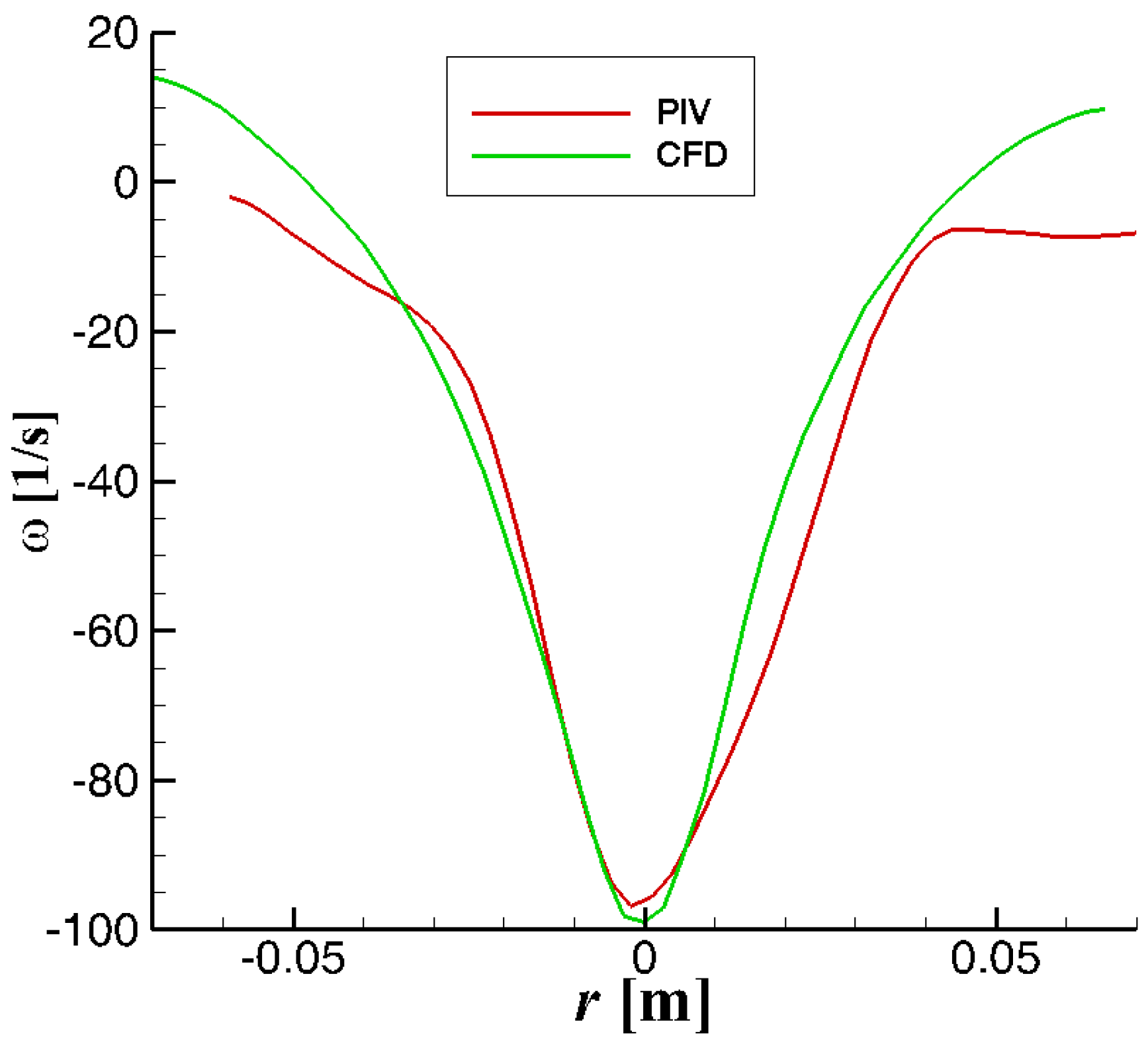
To study the vortex differences, the z = const. sections have been evaluated when the section intersects the vortex center and the distance from the center r is considered. In Figure 32, the graphs are shown for both experimental and mathematical modeling.
The comparison shows a relatively good coincidence of the vorticity in the vortex core; however, outside the vortex core, for |r| > 0.04 m, the difference becomes important.
To quantify the difference between the distributions, the integral over the considered zone (rectangular) was evaluated Iω, which corresponds to the equivalent circulation. For the PIV data, IωPIV = −0.1783 m2/s, and for the CFD data, IωCFD = −0.0434 m2/s. The difference is rather important; it is clear that CFD underestimates the vorticity value, especially outside the vortex core. Within the vortex core, ±0.03 m around the vortex center, the agreement of the mathematical modeling results with experiments is much better; the difference is below 3%.
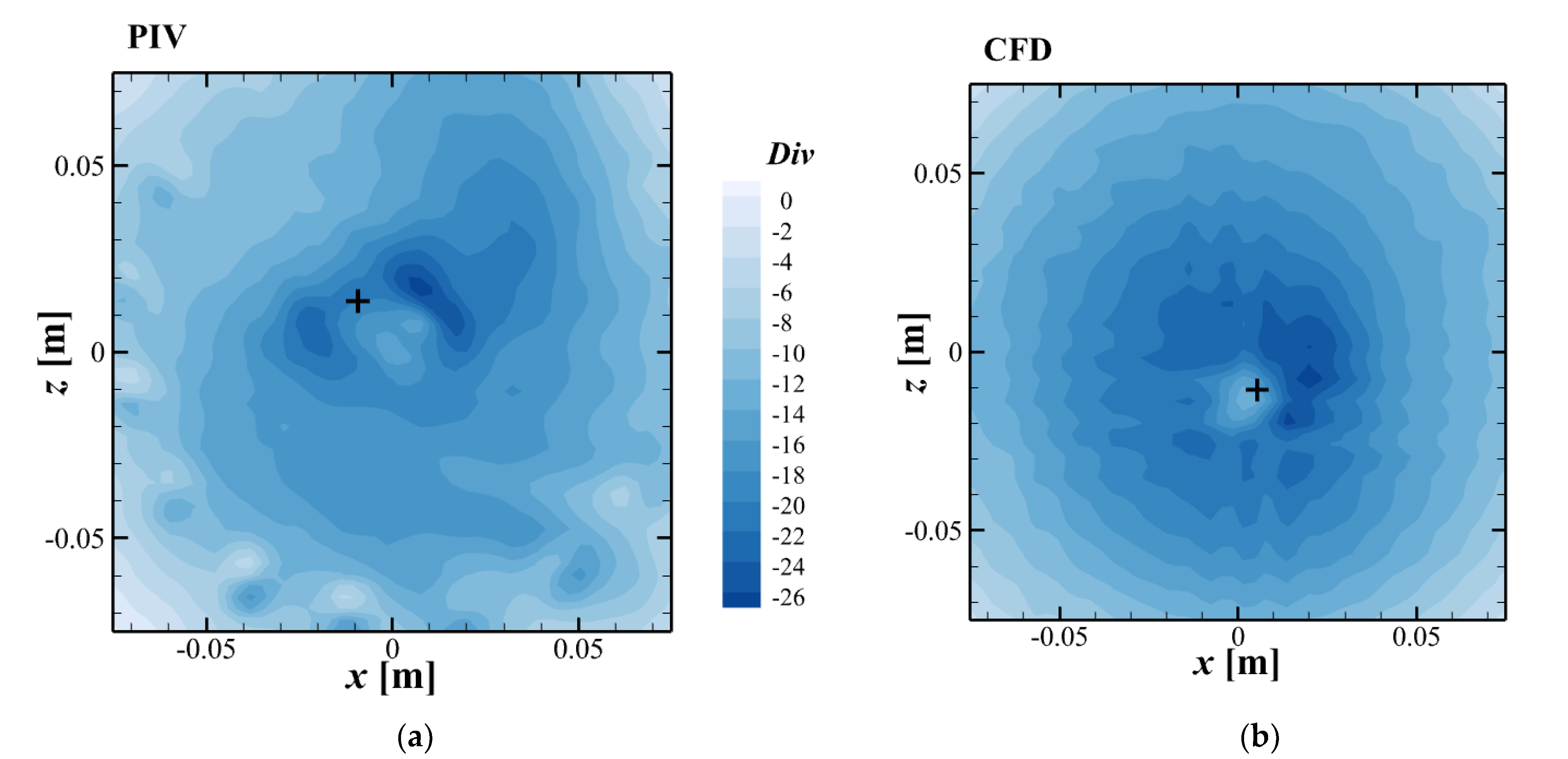
To better estimate the differences between the flow-field topologies, the divergence D has been evaluated for both PIV and CFD data. The 2D definition of the divergence is taken into account:
The flow is incompressible, so the divergence in 3D representation should vanish. Then, the following should hold:
Thus, the evaluated divergence provides information about the out-of-plane velocity component v derivative in its direction y. The topologies of Divergence D for PIV and CFD results are shown in Figure 33.
As the values of divergence are negative everywhere, this result indicates accelerating flow in the y-direction.
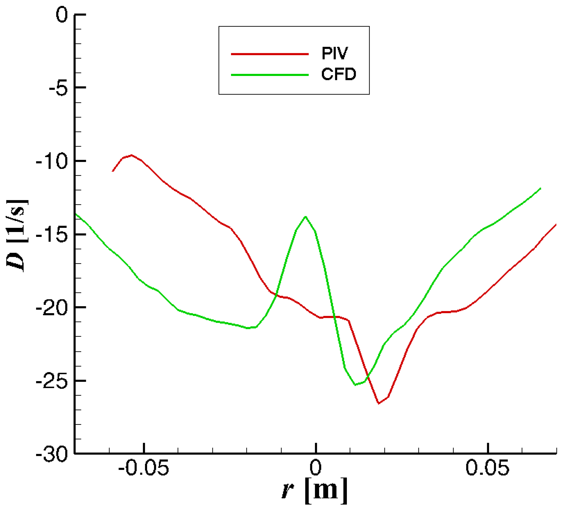
The comparison of divergence in the z = const. section has been evaluated, and the distance from the center r is considered in Figure 34. The difference in the divergence distributions is rather important and visible both in the distribution topology and central section.
The integral of divergence over the considered zone was evaluated ID, which corresponds to the equivalent circulation. For the PIV data, IDPIV = −0.3500 m2/s, and for the CFD data, IDCFD = −0.3034 m2/s. The integral values do not differ very much.
6. Discussion
The main task of this article was to validate the mathematical model adjusted to perform CFD simulation of inlet objects of the pump. The second goal was to study the vortex dynamics using both the visualization technique and PIV measurements.
Generally, it can be said that the bottom (submerged) vortex is present throughout the running of the pump. The detected position of the time-averaged vortex core slightly differs from the PIV and CFD data. However, the topology and vortex dimension were determined very much the same for both approaches.
The free-surface vortex is very hard to study quantitatively (and also visualize) as the existence of such a structure is random both in appearance and behavior, and it is limited in time. Very often, only the swirl of the flow is present. The vortex with a full air core is present less than half the time of the device’s operation. Sometimes even two distinct free-surface vortices were observed. The occurrence of such structures seems to be completely random. The extent, orientation and location determined from the CFD data matches very well with the PIV data in terms of the averaged dataset, at least for time-mean structures.
The path of the vortex core does not show any regular or even pseudo-regular trajectory for the surface vortex and for the submerged one. The free-surface vortex moves with a velocity about three or four times higher than the bottom vortex.
7. Conclusions
The appearance and behavior study on flow in a pump inlet sump is presented.
The vortical structures were studied in detail, and both mathematical modeling and experimental research methods were applied. The advanced unsteady approach has been applied for mathematical modeling to model the flow-field dynamics. For experiments, the time-resolved PIV method has been used.
Three types of dominant vortical structures have been detected: surface vortices, wall-attached vortices and the bottom vortex. The most intense and stable is the bottom vortex. The surface and wall-attached vortices are found to be of random nature as for their appearance and topology; they appear intermittently in time with various topologies. The dominant bottom vortex is relatively steady with weak dynamics. The frequencies of pseudo-periodical behavior were detected up to 1 Hz.
The mathematical modeling has been validated against the experimental data. The bottom vortex core circulation was modeled with an error below 3%. The rest of the flow field was validated qualitatively only. The flow patterns, especially the vortices detected in experiments, are well captured by mathematical modeling.
The origin of the vorticity of all big vortical structures was identified in the pump propeller rotation.
Author Contributions
Conceptualization, M.S. and V.U.; experimental setup design, M.S. and P.P.; validation, P.P., V.U. and M.S.; CFD computation, M.S.; experiments execution, P.P., V.U., M.S. and M.K.; vortex analysis, D.D. and V.U.; writing—original draft preparation, P.P. and V.U.; writing—review and editing, P.P., V.U., M.S. and M.K.; visualization, M.S.; project administration, M.S. and V.U.; funding acquisition, V.U. All authors have read and agreed to the published version of the manuscript.
Funding
The authors thank the Institute of Thermomechanics, Academy of Sciences of the Czech Republic, for funding by the institutional support RVO: 61388998.
Data Availability Statement
The experimental and CFD datasets can be provided by authors on demand.
Acknowledgments
This research was supported by the Czech Ministry of Education, Youth and Sports, grant number CZ.02.1.01/0.0/0.0/17_049/0008408.
Conflicts of Interest
The authors declare no conflict of interest.
Abbreviations
| CFD | Computational Fluid Dynamics |
| FoV | Field of View |
| IA | Interrogation Area |
| POD | Proper Orthogonal Decomposition |
| PoM | Plane of Measurement |
| PIV | Particle Image Velocimetry |
| OPD | Oscillation Pattern Decomposition |
| SST | Shear Stress Transport |
| TKE | Turbulent Kinetic Energy |
| URANS | Unsteady Reynolds-Averaged Navier-Stokes equation |
| VoF | Volume of Fluid |
References
- Domfeh, M.K.; Gyamfi, S.; Amo-Boateng, M.; Andoh, R.; Ofosu, E.A.; Tabor, G. Free surface vortices at hydropower intakes: A state-of-the-art review. Sci. Afr. 2020, 8, e00355. [Google Scholar] [CrossRef]
- Kim, C.G.; Kim, B.H.; Bang, B.H.; Lee, Y.H. Experimental and CFD analysis for prediction of vortex and swirl angle in the pump sump station model. IOP Conf. Ser. Mater. Sci. Eng. 2015, 72, 42044. [Google Scholar] [CrossRef] [Green Version]
- Park, I.; Kim, H.-J.; Seong, H.; Rhee, D.S. Experimental Studies on Surface Vortex Mitigation Using the Floating Anti-Vortex Device in Sump Pumps. Water 2018, 10, 441. [Google Scholar] [CrossRef] [Green Version]
- Okamura, T.; Kamemoto, K.; Matsui, J. CFD prediction and model experiment on suction vortices in pump sump. In Proceedings of the 9th Asian International Conference on Fluid Machinery, Jeju, Korea, 16–19 October 2007. [Google Scholar]
- Gupta, S.; Panda, J.P.; Nandi, N. A model study of free vortex flow. In Proceedings of the ICTACEM, Kharagpur, India, 29–31 December 2014. [Google Scholar]
- Nagahara, T.; Sato, T.; Okamura, T. Effect of the Submerged Vortex Cavitation Occurred in Pump Suction Intake on Hydraulic Forces of Mixed Flow Pump Impeller. In Proceedings of the Fourth International Symposium on Cavitation, Pasedena, CA, USA, 20–23 June 2001. [Google Scholar]
- Amin, A.; Kim, B.H.; Kim, C.G.; Lee, Y.H. Numerical Analysis of Vortices Behavior in a Pump Sump. IOP Conf. Ser. Earth Environ. Sci. 2019, 240, 32020. [Google Scholar] [CrossRef]
- Sedlář, M.; Procházka, P.; Komárek, M.; Uruba, V.; Skála, V. Experimental Research and Numerical Analysis of Flow Phenomena in Discharge Object with Siphon. Water 2020, 12, 3330. [Google Scholar] [CrossRef]
- Papierski, A.; Błaszczyk, A.; Kunicki, R.; Susik, M. Surface Vortices and Pressure in Suction Intakes of Vertical Axial-Flow Pumps. Mech. Mech. Eng. 2012, 16, 51–71. [Google Scholar]
- Bayeul-Lainé, A.C.; Bois, G.; Issa, A. Numerical simulation of flow field in water-pump sump and inlet suction pipe. IOP Conf. Ser. Earth Environ. Sci. 2010, 12, 12083. [Google Scholar] [CrossRef] [Green Version]
- Long, N.I.; Shin, B.R.; Doh, D.-H. Study on Surface Vortices in Pump Sump. J. Fluid Mach. 2012, 74, 60–66. [Google Scholar] [CrossRef]
- Shin, B. Numerical Study of Effect of Flow Rate on Free Surface Vortex in Suction Sump. Trans. Jpn. Soc. Comput. Eng. Sci. 2018, 2018, 20180010. [Google Scholar]
- Tokyay, T.; Constantinescu, G. Coherent structures in pump-intake flows: A large eddy simulation (LES) study. In Proceedings of the Korea Water Resources Association Conference, Seoul, Korea, 11–16 September 2005; pp. 231–232. [Google Scholar]
- Sokolovskiy, M.A.; Carton, X.J.; Filyushkin, B.N. Mathematical Modeling of Vortex Interaction Using a Three-Layer Quasigeostrophic Model. Part 2: Finite-Core-Vortex Approach and Oceanographic Application. Mathematics 2020, 8, 1267. [Google Scholar] [CrossRef]
- Uruba, V. Decomposition methods in turbulent research. Eur. Phys. J. Conf. 2012, 25, 1095. [Google Scholar] [CrossRef] [Green Version]
- Uruba, V. Near Wake Dynamics around a Vibrating Airfoil by Means of PIV and Oscillation Pattern Decomposition at Reynolds Number of 65,000. J. Fluids Struct. 2015, 55, 372–383. [Google Scholar] [CrossRef]
- ANSYS Inc. ANSYS CFX-Solver Theory Guide; Release 19.2; ANSYS Inc.: Canonsburg, PA, USA, 2019. [Google Scholar]
- Zwart, P.J.; Gerber, A.G.; Belamri, T. A Two-Phase Flow Model for Predicting Cavitation Dynamics. In Proceedings of the ICMF 2004 International Conference on Multiphase Flow, Yokohama, Japan, 30 May–3 June 2004. [Google Scholar]
- Joa, J.C.; Kanga, D.G.; Kima, H.J.; Roha, K.W.; Yunea, Y.G. The Effect of Coriolis Force on the Formation of Dip on the Free Surface of Water Draining from a Tank. In Proceedings of the Transactions of the Korean Nuclear Society Autumn Meeting, Pyeongchang, Korea, 25–26 October 2007. [Google Scholar]
- Menter, F.R.; Egorov, Y. A scale-adaptive simulation model using two-equation models. In Proceedings of the 43rd AIAA Aerospace Sciences Meeting and Exhibit, Reno, NV, USA, 10–13 January 2005. [Google Scholar] [CrossRef]
- Menter, F.R.; Schutze, J.; Kurbatskii, K.A. Scale-Resolving Simulation Techniques in Industrial CFD. In Proceedings of the 6th AIAA Theoretical Fluid Mechanics Conference, Honolulu, HI, USA, 27–30 June 2011. [Google Scholar] [CrossRef]
Figure 1.
Construction drawings of test stand (a), description of the test section, coordinates definition (b), top view with dimensions (c).
Figure 1.
Construction drawings of test stand (a), description of the test section, coordinates definition (b), top view with dimensions (c).

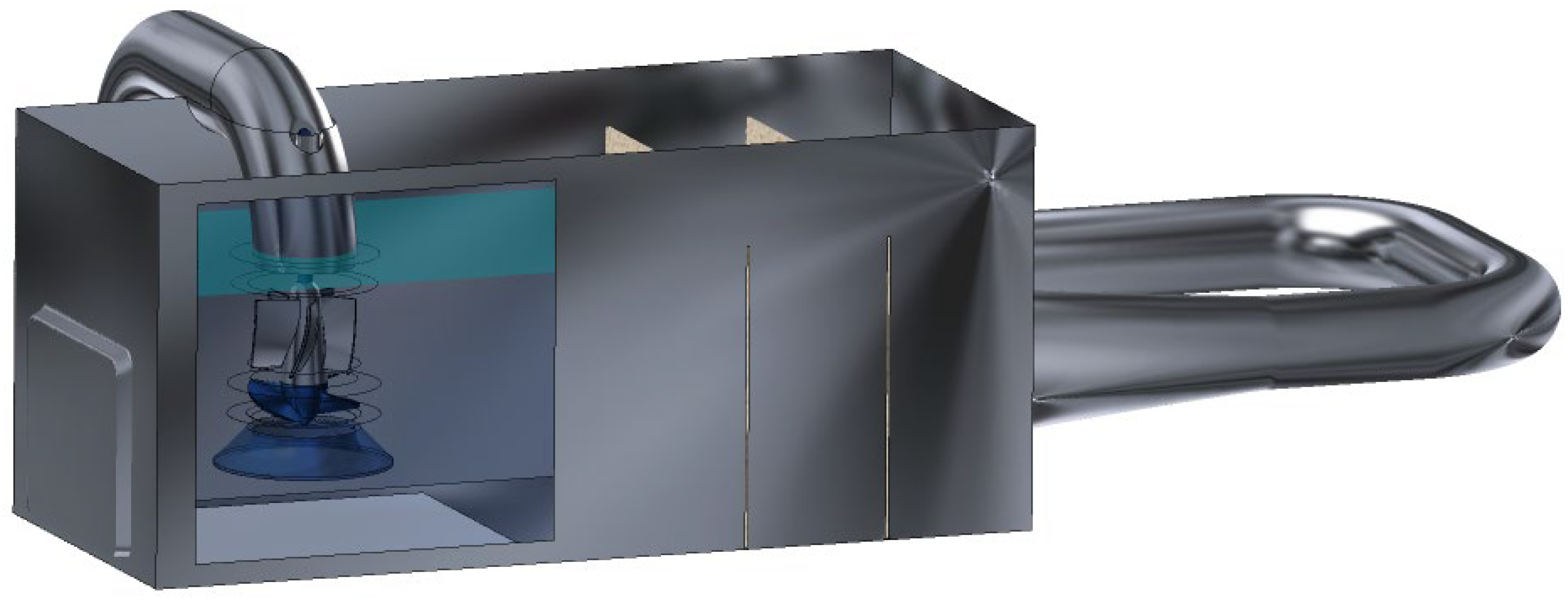
Figure 2.
Experimental stand with rectangular tank and transparent windows. Three-dimensional model used in CFD simulations.
Figure 2.
Experimental stand with rectangular tank and transparent windows. Three-dimensional model used in CFD simulations.

Figure 3.
Detail of axial flow pump input with bellmouth.

Figure 4.
Settling chamber. View of the screens and initial water level.

Figure 5.
View of vortices close to pump suction (a) and singular point movement trail (b).

Figure 6.
Pair of free-surface vortices, (a) side view, (b,c) bottom view.

Figure 7.
PIV setup; vertical (a) and horizontal (b) PoMs, Cartesian coordinate system (c).

Figure 8.
Boundary conditions. CFD.

Figure 9.
Complex system of vortices in the testing tank. Iso-surfaces of constant air volume fraction 5% (in cyan) and constant vapor volume fraction 5% (in grey). CFD.
Figure 9.
Complex system of vortices in the testing tank. Iso-surfaces of constant air volume fraction 5% (in cyan) and constant vapor volume fraction 5% (in grey). CFD.

Figure 10.
Visualization of vortices in the testing tank. Q criterion (in green). CFD.

Figure 11.
Pair of counter-rotating free-surface vortices and bottom vortices. Iso-surfaces of constant air volume fraction 5% (in cyan) and constant vapor volume fraction 5% (in grey). CFD.
Figure 11.
Pair of counter-rotating free-surface vortices and bottom vortices. Iso-surfaces of constant air volume fraction 5% (in cyan) and constant vapor volume fraction 5% (in grey). CFD.

Figure 12.
Vector lines (left) and vorticity distribution (right) in horizontal planes y = 50, 70, 105 and 125 mm. CFD.
Figure 12.
Vector lines (left) and vorticity distribution (right) in horizontal planes y = 50, 70, 105 and 125 mm. CFD.


Figure 13.
Vector lines (left) and vorticity distributions (right) in horizontal planes y = 155, 205 and 255 mm. CFD.
Figure 13.
Vector lines (left) and vorticity distributions (right) in horizontal planes y = 155, 205 and 255 mm. CFD.

Figure 14.
Vector lines (left) and longitudinal velocity distribution (right) in vertical planes z = 0, 62 and 130 mm. CFD.
Figure 14.
Vector lines (left) and longitudinal velocity distribution (right) in vertical planes z = 0, 62 and 130 mm. CFD.

Figure 15.
Vertical planes, distribution of horizontal velocity component (left) and vector lines (right). PIV.
Figure 15.
Vertical planes, distribution of horizontal velocity component (left) and vector lines (right). PIV.


Figure 16.
Horizontal plane positions, y = 50, 70, 105, 125 and 155 mm.

Figure 17.
Bottom vortex, y = 50 mm, (a) mean velocity distribution, (b) vector lines, (c) instantaneous vorticity, (d) mean vorticity distributions. PIV.
Figure 17.
Bottom vortex, y = 50 mm, (a) mean velocity distribution, (b) vector lines, (c) instantaneous vorticity, (d) mean vorticity distributions. PIV.

Figure 18.
Bottom vortex evolution towards the impeller in the y-direction, horizonral planes y = 70 (a), 105 (b), 125 (c) and 155 (d) mm. PIV.
Figure 18.
Bottom vortex evolution towards the impeller in the y-direction, horizonral planes y = 70 (a), 105 (b), 125 (c) and 155 (d) mm. PIV.

Figure 19.
The averaged flow topology of the free-surface vortex at y = 155 (a), 205 (b), 255 (c) and 305 (d) mm. PIV.
Figure 19.
The averaged flow topology of the free-surface vortex at y = 155 (a), 205 (b), 255 (c) and 305 (d) mm. PIV.


Figure 20.
Instantaneous snapshots of the surface vortex at y = 205 (a) and 305 (b) mm. PIV.

Figure 21.
Bottom vortex core path at z = 50 mm. PIV.

Figure 22.
1. POD mode at y = 70 mm, vorticity distribution and vector lines. PIV.

Figure 23.
Surface vortex core path at z = 205 mm. PIV.

Figure 24.
POD modes 1 (a), 2 (b)and 3 (c) at y = 205 mm, vorticity distributions and vector lines. PIV.
Figure 24.
POD modes 1 (a), 2 (b)and 3 (c) at y = 205 mm, vorticity distributions and vector lines. PIV.

Figure 25.
Kinetic energy fraction of the first 10 POD modes for both types of vortices.

Figure 26.
Mean fields at y = 70 mm, (a) velocity field, (b) TKE distribution. PIV.

Figure 27.
OPD spectrum, the nine cyclostationary OPD modes.

Figure 28.
The first OPD mode topology, (a) real part, (b) imaginary part.

Figure 29.
Real parts of higher OPD modes topology, (a) OPD 2, (b) OPD 4 and (c) OPD 5.

Figure 30.
Topology of the bottom vortex. (a) PIV, (b) CFD.

Figure 31.
Vorticity distribution, (a) PIV, (b) CFD.

Figure 32.
Vorticity profiles intersecting the vortex, PIV and CFD.

Figure 33.
Divergence distribution (a) PIV, (b) CFD.

Figure 34.
Divergence distribution, PIV (red), CFD (green).

Publisher’s Note: MDPI stays neutral with regard to jurisdictional claims in published maps and institutional affiliations. |
© 2022 by the authors. Licensee MDPI, Basel, Switzerland. This article is an open access article distributed under the terms and conditions of the Creative Commons Attribution (CC BY) license (https://creativecommons.org/licenses/by/4.0/).
Share and Cite
MDPI and ACS Style
Uruba, V.; Procházka, P.; Sedlář, M.; Komárek, M.; Duda, D. Experimental and Numerical Study on Vortical Structures and Their Dynamics in a Pump Sump. Water 2022, 14, 2039. https://doi.org/10.3390/w14132039
AMA Style
Uruba V, Procházka P, Sedlář M, Komárek M, Duda D. Experimental and Numerical Study on Vortical Structures and Their Dynamics in a Pump Sump. Water. 2022; 14(13):2039. https://doi.org/10.3390/w14132039
Chicago/Turabian StyleUruba, Václav, Pavel Procházka, Milan Sedlář, Martin Komárek, and Daniel Duda. 2022. "Experimental and Numerical Study on Vortical Structures and Their Dynamics in a Pump Sump" Water 14, no. 13: 2039. https://doi.org/10.3390/w14132039
Note that from the first issue of 2016, this journal uses article numbers instead of page numbers. See further details here.