Bioretention Systems Optimization and Design Characterization Model Using Fuzzy Rough Set Theory

Abstract

Urban stormwater has become a persistent concern on a global scale due to its adverse environmental implications. It is the prime vector of aquatic contaminants worldwide that causes pollutants when water bodies drain. Bioretention systems are increasingly used to alleviate setbacks associated with stormwater run-off in urban locales. It has played a substantial role in the implementation of low impact development (LID), a concept that addresses urban stormwater problems caused by land changes and development. The use of LID technologies is an innovative approach. However, it is beset with challenges, such as the insufficiency of data on rainfall distribution and difficulty in interpreting data. To address these research gaps, the present study developed a fuzzy rough set data algorithm for bioretention systems. Event mean concentration calculations and fuzzification of rainfall were performed to produce a rough set-based decision rule. Using the Weibull probability distribution, fuzzification of rainfall and parameter data, rule induction, and Preece testing, bioretention design considerations were determined. The bioretention characterizations generated evident pollutants present in the catch basin before and after filtration. In addition, the bioretention characterization conducted in this study was able to reduce the number of tests needed for rainfall identification based on the different attributes.

1. Introduction

The advent of urbanization has brought forth a multitude of advantages manifested through the creation of employment opportunities, modernization, and better access to education and other life-enhancing facilities. While well-planned and efficiently managed urban centers have stood as a cradle for economic growth and better living conditions, they have also instigated environmental setbacks [1]. To sustain the ever-increasing population in urban areas, natural areas have been converted into hard, impervious surfaces, such as roads, driveways, and parking lots [2]. Water-resistant materials, such as concrete, asphalt, and brick stone, cover these hard surfaces rendering them impermeable to water, which in turn, translate into serious environmental implications, such as watershed hydrology alteration, increased risk of flooding, pollution of water bodies, increased rate and peak flow of stormwater run-off [3,4,5], and reduced time to peak flow during flash flood events. Among these setbacks, stormwater run-off has become a persistent global concern, being the leading vector of aquatic pollutants worldwide [3,6,7]. Due to its adverse impacts and the pressing need for sounder use of this water source, various stormwater treatment technologies and management strategies have been developed, including rain gardens, bioswales, permeable pavements, green roofs, and bioretention cells [7].

Bioretention has emerged as one of the most widely used stormwater management strategies in urban locales [4,7,8]. Its underpinnings lie in the early 1990s when it was established as a component of the low impact development (LID) concept, which addresses urban stormwater problems associated with land changes and development [5,9]. Bioretention systems are situated in strategic locations, so as to receive the first-surge run-off from any rainfall event, allowing the system to hold a sizeable volume of run-off from rainfall episodes transpiring for several hours. As applied in urban watersheds, bioretention has been beneficial in reducing loads of pollutants, such as nutrients, heavy metals, suspended solids, hydrocarbons, and pathogenic bacteria [10,11,12]. Other evenly significant advantages have also been documented, including: (1) improved groundwater recharge and baseflow; (2) decreased peak volume; (3) stream channel protection; (4) thermal pollution reduction; (5) protection of ecosystem integrity; (6) facilitation of nutrient cycling; (7) air quality enhancement; (8) urban climate change mitigation [8,11,13].

Local rainfall distribution largely influences the performance of bioretention systems. In order to design a functional and efficient bioretention system, rigorous collection, analysis and proper interpretation of localized data on total rainfall depth, rainfall intensity, and run-off quality over the years have to be carried out. Categorization and fuzzification of the rainfall data will be useful in simplifying LID studies, making data interpretation more accessible. The fuzzy optimization model normalizes the component data information and generates a model of the operation, which allows for the data to be comparable to other studies [14].

To improve the water system in urban areas and manage the increasing concerns regarding urban stormwater run-off, the concept of LID is also applied in the Philippines [15]. The basic management design includes controlling excess water in the form of surface run-off, using it for alternative purposes and improving the water quality. The use of LID technologies has been an innovative approach. However, a paucity of needed information, such as rainfall distribution, difficulty in data interpretation, and the number of tests needed to be carried out, limit the implementation and application of this technology.

1.1. The Growing Concern about Urban Stormwater Run-Off

The sprawl of population in urban centers has brought forth massive development in infrastructures, with the conversion of natural areas into impervious surfaces as one of the main upshots [2]. Concomitant with the expansion of impervious cover is the increase in quantity and rate of stormwater run-off. The increase in the extent of impervious surfaces renders the precipitate incapable of infiltrating into the ground, making urban run-off a prime contributor to non-point source pollution [3]. With the shifting context of urbanization and policies on climate and management, pollution associated with stormwater discharge varies from area to area, based on volume and quality. In a naturally functioning environment, only a trivial proportion of precipitation contributes to surface run-off, but as urbanization amplifies, this percentage considerably increases. This run-off typically drains to the nearest river or stream, which in turn, causes the following adverse impacts to the receiving water bodies: altered streamflow [1], disruption of normal hydrologic processes [8], changes in the natural drainage path, increased flood volumes and stormwater run-off, amplified amount of wash-off pollutants affecting water quality [2], water body alteration and biodiversity problems [5]. Other aftereffects of urban run-off have been documented, including stream bank erosion, contamination of drinking water sources, exposure of humans to pathogenic bacteria, and adverse impact on the economy due to beach closures [8]. In view of the mayhem associated with urban run-off, attention has been focused on developing stormwater management strategies, such as bioretention systems.

1.2. Bioretention: Its Concept and Underpinnings

Bioretention, also recognized as bioinfiltration or biofilters, is defined as land-based water quality and water quantity management practice that uses physical, chemical, and biological properties of soils, plants, and microbes for the elimination of pollutants from stormwater run-off [16]. It was first developed in the early 1990s by Prince George’s County, Department of Environmental Resources as a component of the low impact development (LID) concept [4,9]. To compensate for the environmental consequences of land development on hydrological processes and water quality, the LID approach integrates a hydrologically functional site design with pollution deterrence measures. This concept administers stormwater run-off in small, economical landscape features situated on each lot incorporating natural processes, such as infiltration, filtration, sedimentation, adsorption, volatilization, ion exchange, decomposition, phytoremediation, and storage facility [9,11,16]. Examples of LID techniques are rain gardens, bioswales, green roofs, permeable pavements, and bioretention cells [15].

Among the LID practices, bioretention has gained much impetus as more areas grapple with the ecological impacts of urbanization [10]. Bioretention systems draw inspiration from the natural system’s ability to treat waste as a resource. It maximizes the existing physical, chemical, and biological pollutant removal processes found in the soil and flora component of a terrestrial vegetated community [4].

1.3. Bioretention Systems: Design and Function

Bioretention uses soil media and woody and herbaceous plants to reduce pollutant loads from stormwater run-off coming from urban areas [4]. This system is engineered to receive the first-surge run-off from any rainfall event, with an adept capacity to take hold of a sizeable volume of run-off from rainfall episodes persisting over several hours [4,17]. The water that passes through the facility enters either of these routes: (1) infiltrates deeper for groundwater recharge, and (2) collected in subsurface perforated pipes and passed to conventional storm drains [17].

With the linking goal to reduce the quantity and improve the quality of run-off in urban areas, bioretention systems use shallow storage, landscaping, and soil media to collect stormwater before draining to the watershed and adjacent water bodies [4]. The basic design consists of three distinctive layers—filtration, transition, and drainage layers—which mimic the function of the natural environment [11,18]. The initial bioretention system design is much like a depression backfilled with planting soil lined by a thin layer of sand underneath and planted with native grass, shrubs, and various kinds of trees as treatment media [17]. The soil characteristically has a high sand content to facilitate rapid infiltration, with low proportions of silt and clay to render faster attenuation of pollutant loads during infiltration. A thin layer of wood mulch overlays the soil, intended to prevent erosion and excessive desiccation of the soil layer. The system is also installed with grasses, shrubs, and other plant species for water removal through evapotranspiration, effectual infiltration, and pollutant conversion [17]. Plant species utilized in bioretention are chosen based on the following attributes: (1) well-suited to the existing soil and climatic conditions of the area; (2) tolerant to urban disturbance, such as water and air pollutants, fluctuating soil moisture, ponding variations; (3) nutrient removal efficiency [17,19]. Bioretention systems are useful in commercial, industrial, and residential settings. They can also be applied in other functions, such as roadway and institutional developments, community redevelopment, streetscape projects, trailways and parks, which can be designed in accordance with individual areas and site-specific conditions [9]. The expansion of impermeable surfaces in urban locales has led to increased flood volumes, stormwater peak surges and intensified pollutant wash-off, which could drastically degrade the water quality of run-off [12]. Stormwater run-off serves as a vector of pollutants transporting contaminants, such as organic matter, suspended solids, nitrogen, phosphorus, heavy metals, hydrocarbons, sediments, pesticides, and fertilizer effluents, to the receiving watersheds. Bioretention systems have been found to cleanse pollutants of various sorts from infiltrating run-off. Several studies have demonstrated its ability to remove nutrients such as Kjeldahl nitrogen, total nitrogen, phosphorus [12,17], and ammonium [10]. Heavy metals such as copper, lead, zinc, and other contaminants such as oil and grease, suspended solids, hydrocarbons, motor oil, and pathogenic bacteria were also found to be efficiently removed by bioretention facilities [9,10,11]. Despite its proven efficacy, the full potential of bioretention systems is limited by setbacks in data management, such as insufficient and/or imprecise data [16]. This challenge can be addressed by adapting statistical methods to simulate various scenarios in a locale.

1.4. Rough Set Theory: Concept and Uses

The origin of rough set theory dates back to 1982 when Zdzislaw Palwak introduced it as a contemporary mathematical approach to deal with imprecise knowledge [20,21]. It offers efficient methods, tools, and algorithms for establishing covert patterns in data. The concept of a rough set is grounded on the supposition that, contrary to the classical set theory, additional information, knowledge, and data about elements of a set exist [22]. Since its inception, rough set theory has demonstrated the ability to develop computationally efficient and mathematically sound systems to deal with issues of finding patterns from databases, creation of decision rules, data reduction, principal component analysis, and interpretation of inference on the basis of existing data [20]. The first part of the rough set theory is to establish concepts and rules through the categorization of the relational database. The second component is to discover knowledge through sorting the equivalence relation and classification for the target approximation [23].

The advantages of the rough set approach to data analysis have been established, which include: (1) provision of efficient algorithms to find hidden patterns in data; (2) identifying of relationships that would not be established using statistical procedures; (3) finding of minimal sets of data reduction; (4) allowing for the use of both qualitative and quantitative data; (5) assessing data significance; (6) generation of decision rules from available data; (7) easy to understand; (8) offers a forthright interpretation of gathered results [21].

1.5. Rough Set Data Explorer

Rough Set Data Explorer is a software system based on rough set theory and other methods for rule discovery [20] which was developed by the Laboratory of Intelligent Decision Support Systems of the Institute of Computing Science in Poznan [24]. This system is a descendant of RoughDAS and RoughClass systems, which are considered one of the first successful implementations of the rough set theory. The software allows for the application of the variable prediction rough set and the classical model designed by Pawlak to construct approximations. Rough Set Data Explorer is basically comprised of a graphical user interface and a collection of separate computational modules. It is devised to be a user-friendly tool that can be implemented in data exploration and analysis. It is equally useful for beginners and experts, as well as for occasional users who want to perform data analysis [25].

Fuzzy rough set theory as a new and alternate way for processing bioretention data is one of the goals of this study. With numerous rainfall data and various stormwater pollutants prevalent in LID systems, this novel method aims to produce a design characterization model for bioretention areas. The present study mainly seeks to develop a fuzzy rough set data algorithm that can be used in a bioretention system. It also addresses the following specific aims: to develop a design characterization model for the following bioretention areas: Eco-biofilter (EBF), Green Eco-tree filter 1 (GEF1), Green Eco-tree filter 2 (GEF2), Small Constructed Wetlands 1 (SCW1), and Small Constructed Wetlands 2 (SCW2); to utilize Weibull distribution and rough set theory in the data analysis and rules generation of bioretention parameters and rainfall events; to apply the principles of empirical testing to validate the rules generated.

2. Materials and Methods

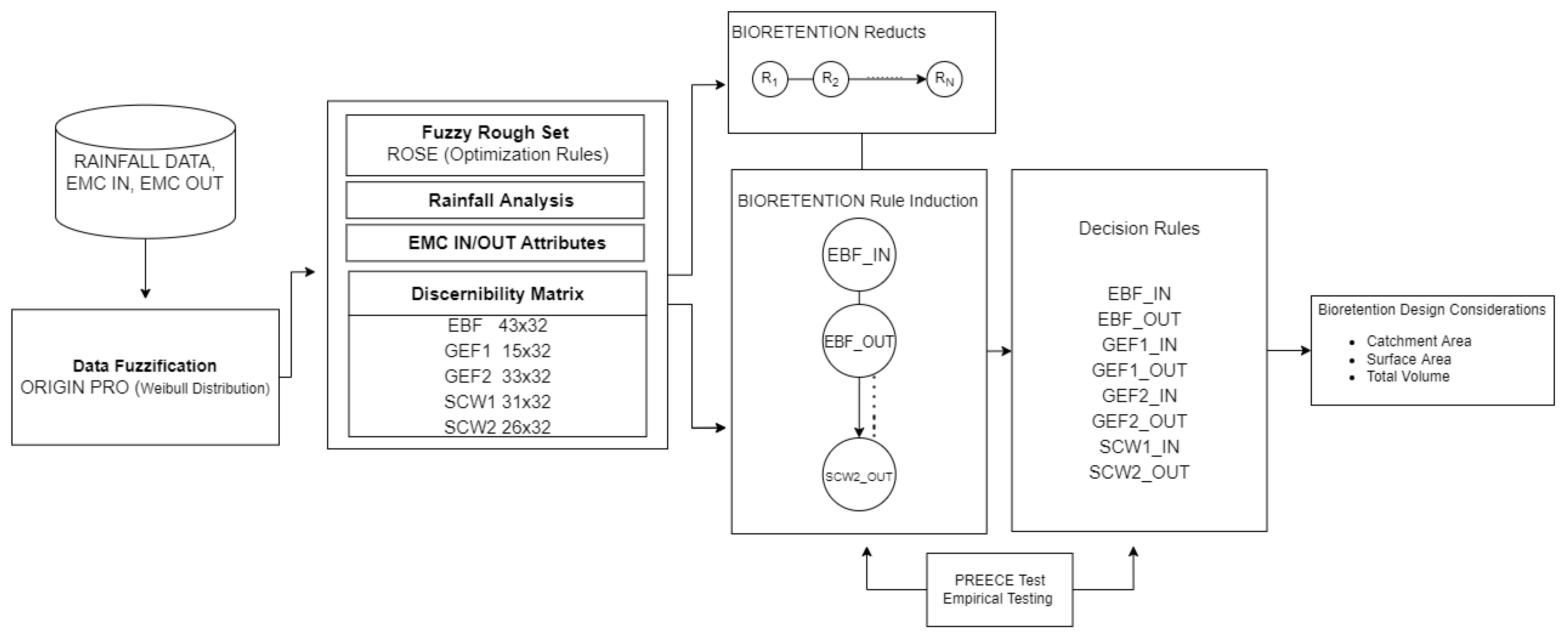
2.1. Methodological Framework

The framework of this research is based on the paper of Sumalatha et. al. [26]. To generate reducts and produce decision rules for forecasting the decision class, researchers employed a rough set-based approach. Figure 1 depicts how decision rules were formulated in the study as the basis for the bioretention design considerations. The data set was derived from the daily records of rainfall amount over thirty years for Cheonan City, Korea. With this range of rainfall values, the fuzzy classifiers method was assigned for the class label [27]. Weibull (Equation (1)) percentages with related precipitation depth were used to assign fuzzy classifiers to rainfall events depending on their intensity. The percentile occurrence frequency of rainfall, which was dependent on the class label, was the object to forecast in the study. The bioretention areas were monitored distinctively resulting in 43, 15, 33, 31, and 26 event mean concentrations for EBF, GEF1, GEF2, SCW1, and SCW2 bioretention, respectively. The entire depth of each rainfall observation event was classified uniquely by assigning a fuzzy value to it. The decision rules were examined using empirical testing.

$$\mathrm{Weibull}\mathrm{formula},P(X>xm)=\left(m\right)/\left(n+1\right)$$

(1)

where: P = percentile ranking, n = total number of the values to be plotted, m = rank of a value in a list ordered by descending magnitude.

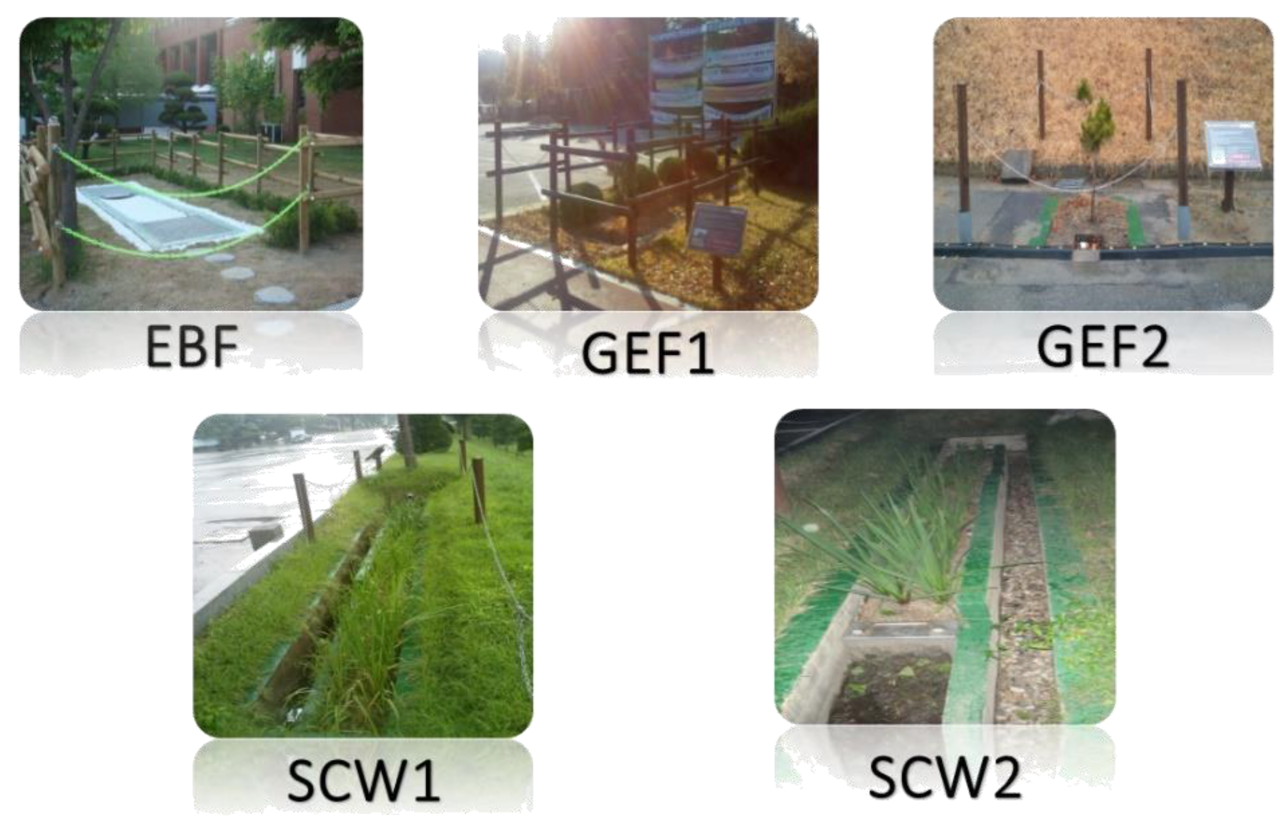
2.2. Research Site Facility

The rainfall data of Kongju National University, Cheonan City, South Chungcheong Province, South Korea (Korean Meteorological Association, 2022 [28]) were one of the study’s inputs, which were constructed in 2014. Rainfall was measured by a local weather station at a regular interval of 1 min, and the weather station data was summed for annual rainfall. For characterization, the rainfall was summed together and shown as annual rainfall data. The percentile occurrence frequency of the rainfall studied ranged from 1st to 10th, 20th, 30th, 40th, 50th, 60th, 70th, 80th, 90th, and 91st to 100th percentile over a normal rainfall, which was analyzed separately using Weibull distribution. The thirty-year (from the year 1990 to 2020) rainfall data was then represented by the average of the percentile occurrence frequency plots for each year. The percentile ranges were recorded and fuzzified by assigning values to each range. There is one percentile difference below the 10th percentile and above the 90th percentile, wherein the ranges were based on the large diversity of rainfall intensities. Additionally, the data were chosen in 10% increments between the 10th and the 90th. The rainfall intensities in the LID systems were fuzzified by assigning values previously obtained by the thirty-year rainfall data. The bioretention rain events were easily classified and processed for use in a fuzzy rough set model. In analyzing the parameters, the manual collection of samples considering the first flush rainwater for analysis at inflow and outflow of each bioretention area was carried out. The sampling frequency was matched to the hydrograph for the rate of water flow in relation to time using a short interval time during the first hour (0, 5, 10, 15, 30, 60 min) and more samples hourly thereafter. The rainwater samples were collected in the EBF bioretention at a specific time interval for both IN and OUT events [27].

2.3. EMC Calculations

Event mean concentration (EMC) attributes and 32 parameters from the Eco-biofilter (EBF), Green Eco-tree filter 1 (GEF1), Green Eco-tree filter 2 (GEF2), Small Constructed Wetlands 1 (SCW1), and Small Constructed Wetlands 2 (SCW2) bioretention areas were measured. EMC characteristics were classified as nutrients, solids, and heavy metals. The parameters determined for each bioretention area were as follows: pH, conductivity, turbidity, total suspended solids (TSS), biochemical oxygen demand (BOD₅), chemical oxygen demand chromium (COD_Cr), chemical oxygen demand manganese (COD_Mn), total organic carbon (TOC), total nitrogen (TN), nitrogen dioxide (NO₂), nitrate (NO₃), ammonium (NH₄), total Kjeldahl nitrogen (TKN), total phosphorus (TP), phosphate (PO₄-P), oil and grease (O&G), chromium (Cr), iron (Fe), nickel (Ni), copper (Cu), zinc (Zn), cadmium (Cd), lead (Pb), total chromium (TCr), total iron (TFe), total nickel (TNi), total copper (TCu), total zinc (TZn), total cadmium (TCd), total lead (TPb), arsenic (As), and total arsenic (TAs).

Table 1. Parameters determined and equipment used in the study.

Parameter	Unit	Equipment
Turbidity	NTU	Turbidity meter: 2100P Portable Turbidimeter by Hach Company, Loveland, CO, USA
Total Suspended Solids (TSS)	mg/L	Drying oven: SJ-201DL by Sejong Scientific Co., Bucheon-si, Korea
Biochemical oxygen demand (BOD5)	mg/L	Incubator: CNC-BIS BOD5 Incubator by Sang San Tech Co., Seoul, Korea
Total nitrogen (TN)	mg/L	UV/VIS spectrometer: Optizen 2120 UV by Mecasys Co., Ltd., Yuseong-gu, Korea
Total Kjeldahl nitrogen (TKN)	mg/L	Kjeldahl machine: KjeltecTM 8200 by Foss, Hillerød, Denmark
Total phosphorus (TP)	mg/L	UV/VIS spectrometer: Optizen 2120 UV by Mecasys Co., Ltd., Yuseong-gu, Korea
Total heavy metals (Cr, Fe, Ni, Cu, Zn, Cd, Pb); Soluble heavy metals (Cr, Fe, Ni, Cu, Zn, Cd, Pb)	mg/L	Sequential plasma spectrometer: ICPS-7510 by Shimadzu Co., Kyoto, Japan

Ref. [29] Maniquiz-Redillas, (2014).

depicts the equipment used in the collection of data for the different parameters. Turbidity, expressed in NTU, was measured using a portable turbidimeter, while total suspended solids (TSS) was determined using a drying oven. Biochemical oxygen demand (BOD₅) for each site was measured using an incubator, whereas concentrations of total nitrogen (TN) and total phosphorus (TP) were obtained through the UV/VIS spectrometer. The bioretention areas were also measured for their total Kjeldahl nitrogen (TKN) content using the Kjeldahl machine, and heavy metals through a sequential plasma spectrometer. TOC-5000A by Shimadzu Co. (Shimadzu Corporation, Kyoto, Japan) was used to analyze TOC. Organic and oxidizable inorganic substances in an aqueous sample are oxidized by potassium dichromate solution in sulfuric acid solution. The excess dichromate is titrated with standard ferrous ammonium sulfate using orthophenanthroline ferrous complex (ferroin) as an indicator. Stormwater run-off samples were collected throughout the storm events and taken to the laboratory for analytical analyses to determine concentrations of common water quality elements in stormwater run-off. The standard test methods for the examination of water and wastewater were used to assess all stormwater run-off samples.

Table 2. Bioretention characterizations.

Characterization	EBF	GEF1	GEF2	SCW1	SCW2
Landuse/Run-off Source	Road	Parking lot		Road/parking lot
Infiltration capability	Yes	Yes	Yes	No	No
Vegetation	No	Yes	Yes	Yes	Yes
Catchment area (m2)	520	880	450	597	457
Ground slope (%)	2.5 ± 1.5	1.3 ± 0.7	0.5 ± 0.5	1.5 ± 0.8	1.9 ± 1.5
Aspect ratio (L:W:H)	1:0.2:0.26	1:1:0.87	1:1:0.87	1:0.15:0.1	1:0.14:0.1
Surface area (m2)	5	2.25	2.25	6.5	7
Total volume (m3)	6.5	2.9	2.93	4.55	4.9
Storage volume (m3)	3.85	1.76	1.76	2.73	2.94
Total cost (USD)	12,200	7650	7650	12,650	16,200

summarizes the five bioretention characteristics. It includes the land use/run-off source, infiltration capability, vegetation, catchment area, ground slope, aspect ratio, surface area, total volume, storage volume, and the total cost. The five bioretention areas vary in terms of land use and run-off source, infiltration capability, presence of vegetation, catchment area, ground slope, surface area, total volume, storage volume, and total cost. The Eco-biofilter (EBF) site has a total catchment area of 520 m², surface area of 5 m², total volume and storage volume of 6.5 m³ and 3.85 m³, respectively. The area is a road devoid of vegetation, able to infiltrate run-off due to its 2.5 ± 1.5% ground slope. The total cost of EBF amounted to USD 12,200. The second area, the Green Eco-tree filter 1 (GEF1) has the largest catchment area of 880 m², with a ground slope of 1.3 ± 0.7%. It has a surface area of 2.25 m², able to hold 2.9 m³, and with a storage volume of 1.76 m³. GEF1 is a parking lot costing USD 7650, surrounded by vegetation allowing it to infiltrate run-off. The third area is the Green Eco-tree filter 2 (GEF2), resembling many attributes of GEF1, except for its smaller catchment area of 450 m² and ground slope of 0.5 ± 0.5 m². The Small Constructed Wetlands 1 (SCW1) is the fourth site, consisting of a road and parking lot surrounded by vegetation with no capacity to infiltrate run-offs. It has a catchment and surface area of 597 m² and 6.5 m², respectively, with a ground slope of 1.5 ± 0.8%. SCW1 has a total volume of 4.55 m³ and a storage volume of 2.73 m³, with a total cost of USD 12,650. The last area is the Small Constructed Wetlands 2 (SCW2), with similar land use, infiltration capacity, and vegetation as that of SCW1. It has a catchment area of 457 m², a surface area of 7 m², and a ground slope of 1.9 ± 1.5%. It can hold a total volume of 4.9 m³ and a storage volume of 2.94 m³. Construction of SCW2 amounted to USD 16,200, the costliest of all the bioretention areas tested [29]. An actual picture of the five bioretentions is shown in Figure 2.

2.4. Event Mean Concentration (EMC)

EMC is a characteristic of run-off concentration statistically used for the inflow and outflow pollutant parameters. It is a significant method to estimate the total emission rate and the contribution of run-off to inflow waters [30,31]. EMC is defined as the total mass load of a certain parameter in a bioretention site during a storm event divided by the total run-off water volume removed in the same storm event [32].

The EMC was calculated using Equation (2):

$$EMC\left(\mathrm{mg}/\mathrm{L}\right)=\frac{M}{V}=\frac{{{\displaystyle \int }}_0^{T}C\left(t\right)\times q_{run}\left(t\right)dt}{{{\displaystyle \int }}_0^T{q}_{run}\left(t\right)dt}\approx \frac{{{\displaystyle \sum }}_0^{t=T}C\left(t\right)\times q_{run}\left(t\right)}{{{\displaystyle \sum }}_0^{t=T}{q}_{run}\left(t\right)}$$

(2)

where M (g) represents the total mass of a pollutant carried during a storm event; V (m³) represents the total volume of run-off; C(t) (mg/L) represents the concentration at time t; q_run(t) represents the run-off flow rate discharged at time t. The time associated with the start and end of run-off is represented by the integration limits t = 0 and t = T, respectively [33].

2.5. Storm Event Monitoring

In analyzing the parameters, manual grab sampling at inflow and outflow of each bioretention area was carried out. The sampling frequency was matched to the hydrograph for the rate of water flow in relation to time using a short time interval during the first hour (0, 5, 10, 15, 30, 60 min) and more samples hourly thereafter. The rainwater samples were collected in the EBF bioretention at a specific time interval for both IN and OUT events.

2.6. Fuzzification of Rainfall and Parameter Datasets

The rainfall events data for both IN and OUT differ from every bioretention. Rainfall events recorded for each bioretention area were as follows: EBF = 43, GEF1 = 15, GEF2 = 33, SCW1 = 31, and SCW2 = 26. These were processed using Weibull probability distribution in OriginPro 2021b software. Each parameter was plotted in which the X and Y-axis showed the actual and predicted cumulative percentage, respectively. A plotted figure for pH for bioretention IN is shown in Figure 3. The upper and lower percentiles were used as a basis of the fuzzified data. The fuzzified rainfall and parameter data were the results of the processed actual values gathered. This novel machine learning method uses software in determining fuzzy values which were used to a greater extent for analyzing systems or applications [21]. The figure shows plotted fuzzy values for pH bioretention IN. The X-axis shows the pH values and the Y-axis represents the Weibull cumulative probability expressed as a percentage. This is the graph result after the fuzzification of data in OriginPro software. The circles represent the percentiles of pH values IN of the different bioretentions. They are referenced with the red line and enclosed by upper and lower percentiles. These percentiles used a 95% confidence band and the results were the basis for the assigning of fuzzy values given the percentile range produced. There were 32 parameters, plus 1 decision rule and 5 bioretentions with 2 events (IN and OUT) having a total of 330 processed tables.

The fuzzy classifiers method was used in assigning a class label to the raw values of the rainfall events [27]. With the five bioretention areas, different rainfall observations were noted. After assigning classifiers, the resulted class label prediction of the object was used for the optimization of rules.

2.7. Rough Set Theory Using Rule Induction

The bioretention fuzzified value attributes were processed in the rough set data explorer (ROSE) software using the rule induction of rough set theory. The EMC parameters’ fuzzy values were coded using the numeric-integer (“number-coded”) data type. The output was set to the rainfall fuzzy value, the series of bioretention parameters were arranged in notepad, and the file was saved from text to isf format. An isf file is needed by the ROSE for the data to be processed. The concept of rough set theory seeks to reduce a given conditional attribute data set to a smaller subset while keeping the reduced subset consistently connected to the conditional attribute [34,35]. If the matching decision attributes for any objects set with equal feature values are comparable, the dataset is deemed consistent. This is accomplished through the formulation of the reducts and core notions in rough set theory. Through the concept of rough set theory using the ROSE software, the enormous EMC parameters fuzzy values data were reduced to a smaller set of rules. These rules were the basis of bioretention design considerations.

3. Results and Discussion

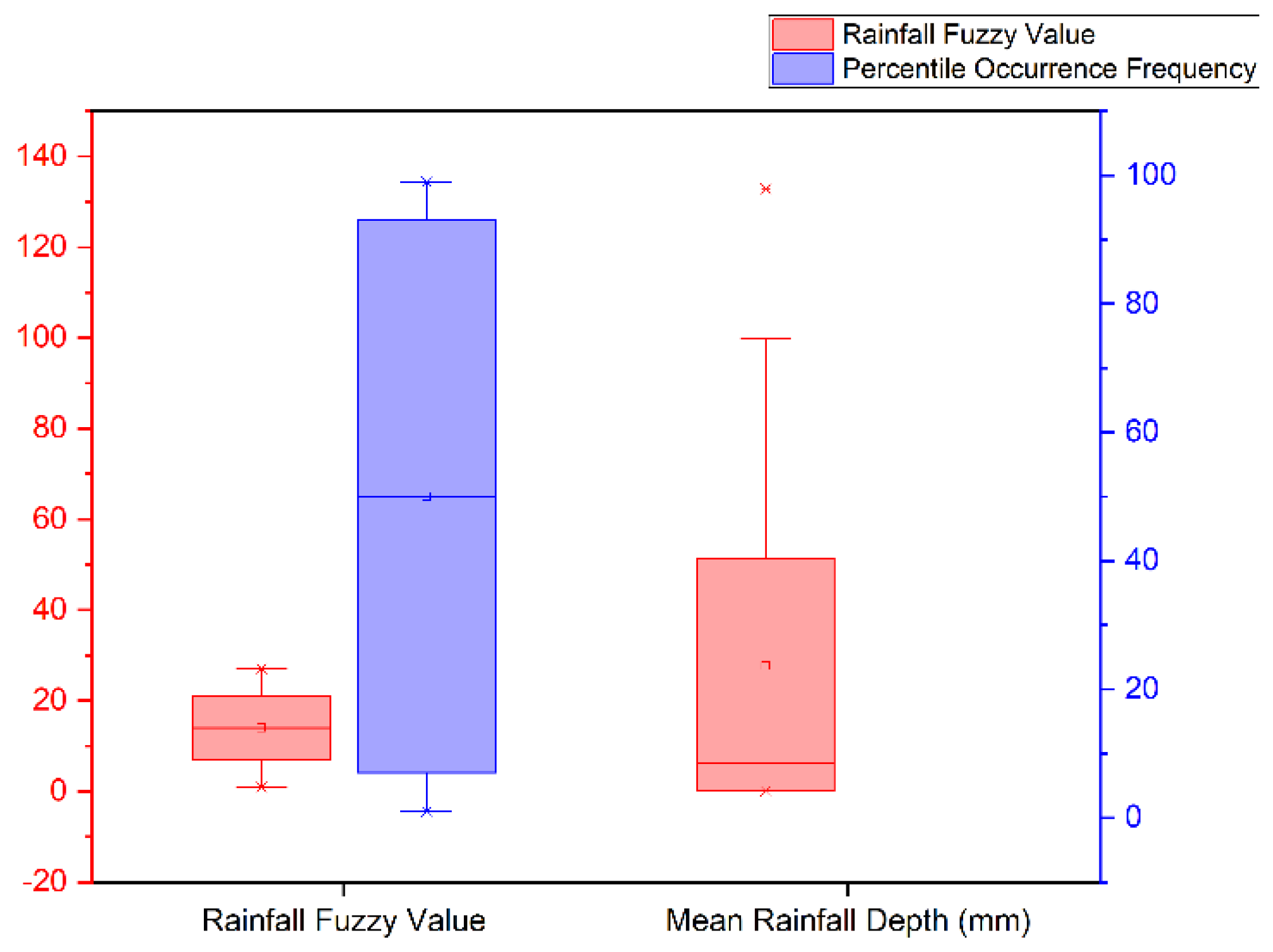
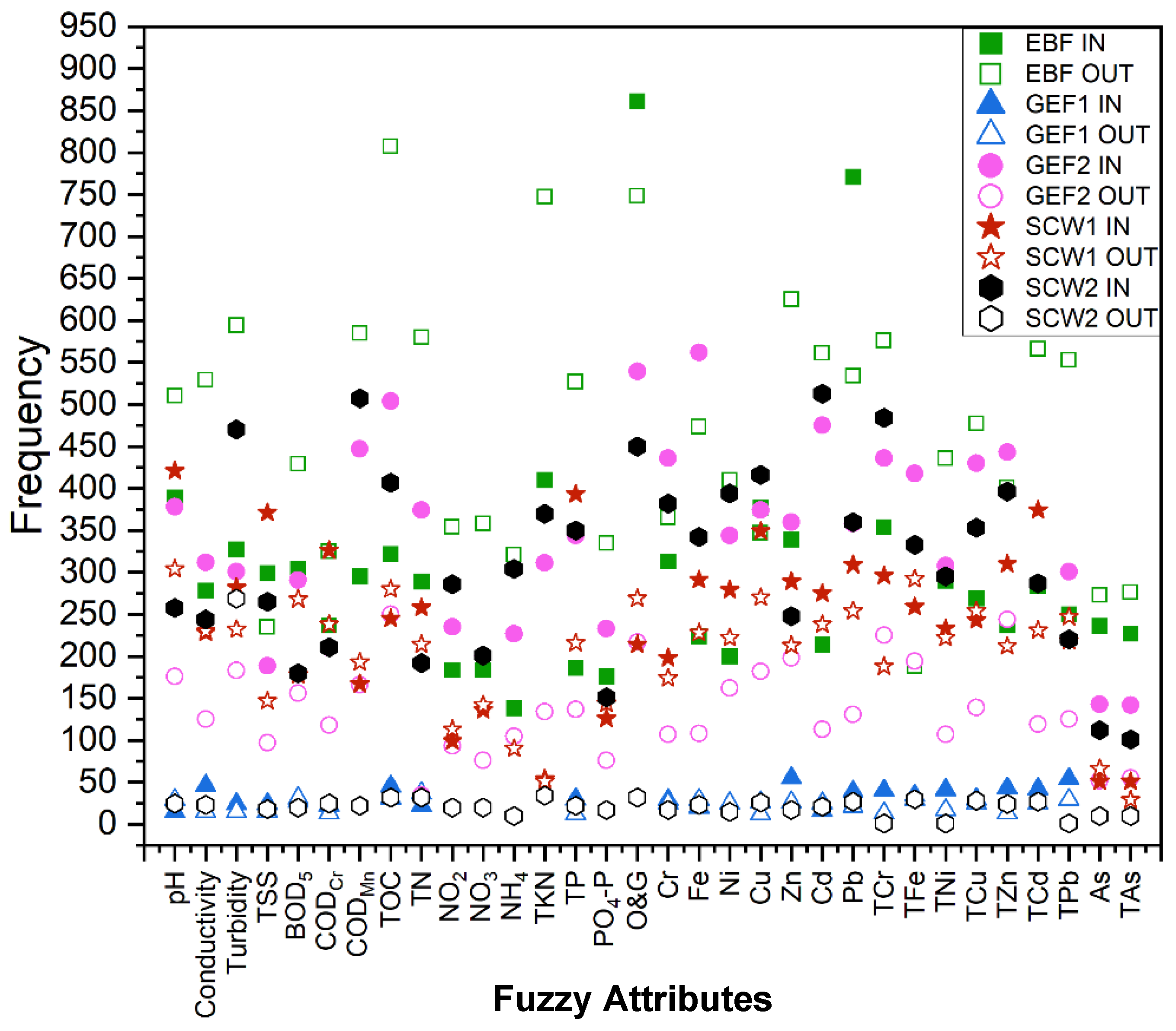
3.1. Fuzzification of Rainfall and EMC Events

Table 3. Groupings of pH and its corresponding fuzzy values.

Bioretention		pH Fuzzy Values
		1–10	11–13	14–16	17–19	20–27
IN	EBF	3.00–5.63	5.64–7.21	7.22–8.93	8.94–10.2	10.2–12.2
	GEF1	5.83–7.09	7.10–7.69	7.70–8.28	8.29–8.68	8.69–9.31
	GEF2	4.55–6.52	6.53–7.49	7.50–8.38	8.39–8.95	8.96–10.5
	SCW1	4.59–6.68	6.69–7.72	7.73–8.68	8.69–9.30	9.31–10.8
	SCW2	5.48–6.88	6.89–7.53	7.54–8.11	8.12–8.49	8.50–9.05
OUT	EBF	4.90–6.54	6.55–7.32	7.33–8.01	8.02–8.45	8.46–9.12
	GEF1	6.46–6.53	6.54–6.57	6.58–6.64	6.65–6.69	6.70–6.78
	GEF2	5.59–6.33	6.34–6.64	6.65–6.93	6.94–7.10	7.11–7.37
	SCW1	5.04–6.70	6.71–7.48	7.49–8.20	8.21–8.65	8.66–9.33
	SCW2	5.03–6.91	6.92–7.83	7.84–8.68	8.69–9.23	9.24–10.1

summarizes the groupings of pH values of the different bioretention systems and their corresponding fuzzy values. Groupings were based on the percentile occurrence frequency of rainfall data. These fuzzy values were used as input values in the rough set data explorer software to process rules.

The various rain intensities and their respective percentile occurrence frequency are shown in Figure 4. This categorization of the mean rainfall was used for the fuzzy values concerning the water depth. These fuzzy values, 1 to 27, correlate to the five bioretention areas for both IN and OUT EMC events, capturing the entire 90th percentile of the total rainfall events as depicted in

Table 4. Percentile Occurrence Frequency.

Rainfall Fuzzy Value	Percentile Occurrence Frequency	Mean Rainfall Depth (mm)
1	1	0.02
2	2	0.05
3	3	0.08
4	4	0.12
5	5	0.16
6	6	0.21
7	7	0.26
8	8	0.32
9	9	0.37
10	10	0.43
11	20	1.22
12	30	2.35
13	40	3.93
14	50	6.13
15	60	9.29
16	70	14.12
17	80	22.34
18	90	40.21
19	91	43.34
20	92	46.97
21	93	51.25
22	94	56.40
23	95	62.80
24	96	71.06
25	97	82.40
26	98	99.72
27	99	132.85

. With the thirty-year rainfall data, Weibull distribution was used to assign each of the fuzzified values to the 3337 rainfall occurrences, resulting in their identified relationship [27].

In producing rough set relation, attributes that have the same values are collected into the same class. These are equivalence classes where objects in the same class are indiscernible. Using the discernibility matrix function of the ROSE software, the method of rule induction substantiated the percent frequency on the number of times the class or the parameter fuzzy value appeared before rule induction. Indiscernibility relation is a set approximation, where it gives us both lower L(X) approximation and upper approximation U(X), hence, calculating the accuracy of approximation α(X). The various parameters and percentile occurrence frequency were considered as a correlation to the discernibility matrix of the bioretention systems. Reducts look for the smallest subset of attributes that allow the same categorization of elements in the original data as the entire set of attributes, in which computing such minimal reducts among all reducts. Figure 5 shows the parameter attributes of the bioretention system reducts. The discernibility matrix creates a reduction in attributes by extracting the less preferred and including those that are more preferred [36].

Table 5. Discernibility matrix of five bioretentions for both IN and OUT.

		% Frequency
Attribute	Unit	EBF IN	EBF OUT	GEF1 IN	GEF1 OUT	GEF2 IN	GEF2 OUT	SCW1 IN	SCW1 OUT	SCW2 IN	SCW2 OUT
FpH		15.1	13.1	4.92	14.1	13.5	12.9	20.5	16.5	9.40	9.29
FConductivity	µs/cm	10.8	13.6	15.1	7.32	11.2	9.18	11.1	12.5	8.89	8.55
FTurbidity	NTU	12.7	15.3	7.87	7.32	10.8	13.4	13.7	12.7	17.1	100
FTSS	mg/L	11.6	6.04	7.87	7.32	6.77	7.12	18.0	7.96	9.65	6.69
FBOD5	mg/L	11.8	11.0	8.85	15.1	10.4	11.5	8.7	14.5	6.56	7.43
FCODCr	mg/L	9.21	8.35	7.21	6.34	7.52	8.66	15.8	12.9	7.69	9.29
FCODMn	mg/L	11.5	15.0			16.0	12.2	8.12	10.5	18.5	8.18
FTOC	mg/L	12.5	20.7	14.8	15.1	18.0	18.4	11.9	15.2	14.8	11.9
FTN	mg/L	11.2	14.9	7.21	18.0	13.4	2.6	12.5	11.6	6.99	11.9
FNO2	mg/L	7.15	9.10			8.41	6.83	4.81	6.12	10.4	7.43
FNO3	mg/L	7.15	9.20			7.20	5.58	6.61	7.69	7.32	7.43
FNH4	mg/L	5.36	8.25			8.13	7.71	4.38	4.88	11.1	3.72
FTKN	mg/L	15.9	19.2			11.1	9.84	2.63	2.76	13.5	12.6
FTP	mg/L	7.23	13.5	9.84	5.85	12.3	10.1	19.1	11.7	12.7	8.18
FPO4-P	mg/L	6.84	8.61			8.34	5.58	6.13	7.80	5.50	6.32
FO&G	mg/L	33.5	19.2			19.3	15.9	10.4	14.6	16.4	11.9
FCr	mg/L	12.2	9.38	9.51	12.2	15.6	7.86	9.63	9.43	13.9	6.32
FFe	mg/L	8.71	12.2	6.56	14.1	20.1	7.93	14.1	12.3	12.5	8.55
FNi	mg/L	7.77	10.5	8.20	12.2	12.3	11.9	13.6	12.0	14.4	5.58
FCu	mg/L	14.7	8.92	8.52	5.85	13.4	13.4	17.0	14.6	15.1	9.67
FZn	mg/L	13.2	16.1	18.0	12.7	12.9	14.5	14.0	11.5	9.03	6.32
FCd	mg/L	8.32	14.4	5.25	12.2	17.0	8.30	13.4	12.9	18.7	7.81
FPb	mg/L	30.0	13.7	12.8	10.2	12.8	9.62	15.0	13.8	13.1	10.0
FTCr	mg/L	13.8	14.8	13.1	6.34	15.6	16.5	14.4	10.2	17.6	0.37
FTFe	mg/L	43.9	4.83	11.1	14.1	15.0	14.2	12.6	15.8	12.1	11.1
FTNi	mg/L	11.3	11.2	13.4	8.29	11.0	7.86	11.3	12.0	10.7	0.37
FTCu	mg/L	10.5	12.3	9.84	12.2	15.4	10.2	11.8	13.8	12.9	10.4
FTZn	mg/L	9.21	10.3	14.1	6.34	15.9	17.9	15.1	11.5	14.4	8.92
FTCd	mg/L	11.0	14.5	13.8	12.2			18.2	12.5	10.5	10.0
FTPb	mg/L	9.72	14.2	17.7	14.1	10.8	9.18	10.6	13.4	8.01	0.37
FAs	mg/L	9.17	7.01			5.12	3.82	2.48	3.58	4.08	3.72
FTAs	mg/L	8.82	7.09			5.08	4.04	2.48	1.57	3.68	3.72
NUMBER OF REDUCTS		2573	3892	305	205	2793	1362	2057	1846	2745	269

exemplifies the frequency or instances the attributes appeared over the total number of reducts, expressed in percentage. The attribute parameter units are also depicted in this table. It can be noted that there are empty values in the table, indicating the unavailability of data for this attribute and type of bioretention. The total number of reducts produced after running the data in the ROSE software is shown in the last row of the table.

3.2. Bioretention Rules Optimization

Basic minimal rule induction of the ROSE software-generated rules as the basis for design considerations of bioretention systems.

Table 6. EBF IN fuzzified values rules optimization.

No.	Rule	Rainfall Fuzzy Value	EMC Parameters	Percentile Occurrence Frequency
1	(FTOC = 19) => (EBF_IN = 11)	EBF_IN = 11	FTOC = 19	20
2	(FTCu = 13) & (FTPb = 13) => (EBF_IN = 12);	EBF_IN = 12	FTCu = 13, FTPb = 13	30
3	(FTSS = 16) & (FTN = 17) => (EBF_IN = 12)	EBF_IN = 12	FTSS = 16, FTN = 17	30
4	(FTurbidity = 24) => (EBF_IN = 12)	EBF_IN = 12	FTurbidity = 24	30
5	(FTSS = 17) & (FCd = 16) => (EBF_IN = 13)	EBF_IN = 13	FTSS = 17, FCd = 16	40
6	(FTurbidity = 21) => (EBF_IN = 13)	EBF_IN = 13	FTurbidity = 21	40
7	(FCr = 3) => (EBF_IN = 13)	EBF_IN = 13	FCr = 3	40
8	(FPb = 13) => (EBF_IN = 13)	EBF_IN = 13	FPb = 13	40
9	(FConductivity = 13) & (FCODCr = 13) => (EBF_IN = 14)	EBF_IN = 14	FConductivity = 13, FCODCr = 13	50
10	(FTSS = 17) & (FTN = 15) => (EBF_IN = 14)	EBF_IN = 14	FTSS = 17, FTN = 15	50
11	(FNO2 = 11) & (FCu = 14) => (EBF_IN = 14)	EBF_IN = 14	FNO2 = 11, FCu = 14	50
12	(FNH4 = 0) & (FTFe = 12) => (EBF_IN = 14)	EBF_IN = 14	FNH4 = 0, FTFe = 12	50
13	(FNO2 = 15) => (EBF_IN = 14)	EBF_IN = 14	FNO2 = 15	50
14	(FTP = 15) & (FO&G = 17) => (EBF_IN = 14)	EBF_IN = 14	FTP = 15, FO&G = 17	50
15	(FNi = 11) & (FTCu = 10) => (EBF_IN = 15)	EBF_IN = 15	FNi = 11, FTCu = 10	60
16	(FBOD5 = 11) & (FTP = 11) => (EBF_IN = 15)	EBF_IN = 15	FBOD5 = 11, FTP = 11	60
17	(FPO4-P = 15) & (FTFe = 12) => (EBF_IN = 15)	EBF_IN = 15	FPO4-P = 15, FTFe = 12	60
18	(FNO2 = 17) => (EBF_IN = 15)	EBF_IN = 15	FNO2 = 17	60
19	(FTKN = 10) & (FTZn = 16) => (EBF_IN = 15)	EBF_IN = 15	FTKN = 10, FTZn = 16	60
20	(FTFe = 15) & (FTCd = 10) => (EBF_IN = 16)	EBF_IN = 16	FTFe = 15, FTCd = 10	70
21	(FpH = 14) & (FTPb = 14) => (EBF_IN = 16)	EBF_IN = 16	FpH = 14, FTPb = 14	70
22	(FTFe = 3) => (EBF_IN = 17)	EBF_IN = 17	FTFe = 3	80
23	(FCODMn = 11) & (FPO4-P = 0) => (EBF_IN = 18)	EBF_IN = 18	FCODMn = 11, FPO4-P = 0	90
24	(FTurbidity = 16) & (FTCr = 16) => (EBF_IN = 18)	EBF_IN = 18	FTurbidity = 16, FTCr = 16	90
25	(FBOD5 = 5) => (EBF_IN = 26)	EBF_IN = 26	FBOD5 = 5	98
26 Approximation Rule	(FTFe = 0) => (EBF_IN = 1) OR (EBF_IN = 13)	EBF_IN = 1) OR (EBF_IN = 13)	FTFe = 0	1 OR 40

depicts the rule for the EBF IN bioretention (complete list of rules optimization tables in Supplementary Tables S1–S9). Considering the rainfall fuzzy value, EMC parameters, and percentile occurrence frequency, results vary indistinctively. Rough set theory produced specific EMC parameters for the corresponding rainfall fuzzy value. Each rule produced is in the form of EMC parameter/s with its corresponding fuzzy value => and the rainfall fuzzy value. Approximation rules appear when there are the same set of conditions, that is when the same condition relates to more than one outcome.

3.3. Preece Test

The data set for the EBF IN bioretention had 43 numbers of rules and were decreased to 26 numbers of rules (as indicated in

Table 7. Percentage decrease in rules generated.

Bioretention		Number of Rules	Number of Reduced Rules	Percentage Decrease
EBF	IN	43	26	39.53
	OUT	44	20	54.55
GEF1	IN	15	11	26.67
	OUT	14	NO RULES GENERATED	00.00
GEF2	IN	33	19	42.42
	OUT	33	13	60.61
SCW1	IN	31	17	45.16
	OUT	31	16	48.39
SCW2	IN	26	16	38.46
	OUT	27	16	40.74

) resulting in a 39.53% decrease. EBF OUT, GEF1 IN, GEF2 In, GEF2 OUT, SCW1 IN, SCW1 OUT, SCW2 IN, and SCW2 OUT has a 54.55%, 26.67%, 42.42%, 60.61%, 45.16%, 48.39%, and 38.46% decreased number of rules, respectively. It can be perceived that there is a significant number difference in the rules after processing. For the GEF1 OUT bioretention, there were no reduced rules generated as the data gathered showed insignificant numbers that cannot be processed by the ROSE software. Upon checking manually, most data attributes for this bioretention were zeros.

It was found that the percent validity computed was 100 percent after applying empirical testing to the rules developed. The total number of rules produced by the ROSE software was tallied and variable a was assigned to it. Each rule produced by this expert system algorithm was checked with the fuzzified rough set values to determine if the values matched. The number of rules where the values of the percentile occurrence frequency and EMC parameters matched the fuzzy values were counted and assigned to variable b. To compute the percent validity c, the formula: c = (b/a) times 10 was used. In performing this test, half of the data were to be used in model building and the other half were for the data invalidation. Using empirical testing, the principles derived by the rough set theory were valid [37].

3.4. Bioretention Design Considerations

The summary of the critical parameters as the basis for the bioretention design considerations is given in

Table 8. Critical fuzzified parameters present before and after filtration.

Bioretention	Catchment Area (m2)	Surface Area (m2)	Total Volume (m3)	Storage Volume (m3)	EMC Parameters IN	EMC Parameters OUT
EBF	520	5	6.5	3.85	FpH = 14, Fconductivity = 13, Fturbidity = 24, FTSS = 17, FBOD5 = 11, FCODCr = 13, FCODMn = 11, FTOC = 19, FTN = 17, FNO2 = 17, FNH4 = 0, FTKN = 10, FTP = 15, FPO4-P = 15, FO&G = 17, FCr = 3, Fni = 11, Fcu = 14, FCd = 16, FPb = 13, FTCr = 16, FTFe = 12, FTCu = 13, FTZn = 16, FTCd = 10, FTPb = 14	FpH = 19, Fconductivity = 21, Fturbidity = 5, FTSS = 17, FBOD5 = 13, FCODCr = 10, FTOC = 10, FTN = 11, FNH4 = 19, FTKN = 12, FTP = 15, Fni = 17, FZn = 12, FTCr = 15, FTFe = 15, FTNi = 12, Fas = 0
GEF1	880	2.25	2.9	1.76	FpH = 21, Fconductivity = 21, Fturbidity = 1, FTSS = 13, FTOC = 2
GEF2	450	2.25	2.93	1.76	FpH=17, Fconductivity = 26, FTSS = 18, FBOD5 = 2, FCODCr = 14, FTOC = 9, FTKN = 0, FTP = 12, FO&G = 11, FCr = 13, Ffe = 11, FZn = 10, FPb = 16, FTFe = 13, FTNi = 12, FTZn = 16, FTAs = 0	FpH = 21, Fconductivity = 10, Fturbidity = 17, FTSS = 16, FBOD5 = 12, FTN = 9, FTKN = 0, FPb = 10, FTCr = 13
SCW1	597	6.5	4.55	2.73	FpH = 21, FTSS = 15, FBOD5 = 20, FCODCr = 16, FTOC = 11, FTN = 12, FO&G = 13, FCr = 12, FTNi = 0, FTZn = 10, FTPb = 15	FpH = 19, Fconductivity = 16, Fturbidity = 13, FTSS = 11, FCODCr = 8, FTN = 13, Fcu = 13, FTCr = 14, FTFe = 13, FTNi = 11, FTCu = 13
SCW2	457	7	4.9	2.94	FpH = 19, Fconductivity = 21, Fturbidity = 13, FTSS = 17, FBOD5 = 13, FCODCr = 14, FTOC = 10, FTN = 11, FNO2 = 10, FNH4 = 19, FTKN = 12, FTP = 15, Fni = 17, FZn = 12, FTCr = 15, FTFe = 15, FTNi = 15, FTAs = 0	FpH = 0, Fconductivity = 25, Fturbidity = 8, FTSS = 16, FTOC = 17, FTN = 9, FNH4 = 0, FTKN = 11, FTP = 12, FO&G = 10, FZn = 13, FTNi = 0, FTCu = 10, FTPb = 0

. The EMC parameters IN and OUT were the resulted fuzzy values considering the 1st–90th percentile as rainfall was imminent at this level [27]. Based on the recorded observations, it was at these percentiles that the maximum rainfall was captured. The EMC parameters IN are the evident pollutants present in the bioretention system in the catch basin. The EMC parameters OUT are the resulted pollutants appearing in the corresponding bioretention system after filtration has been generated. The catchment area, surface area, total volume, and storage volume for EBF bioretention were 520 m², 5 m², 6.5 m³, and 3.85 m³, respectively. For this type of bioretention, the following observations were expected: out of the 32 parameters, only 26 will be significantly present given the amount of the rainfall occurrence frequency; after filtration, only 17 parameters are projected to be significant. For the GEF1, GEF2, SCW1, and SCW2 bioretention, the catchment area, surface area, total volume, and storage volume are depicted in Table 8. Some of the pH values displayed are over 14, which is the result of the parameters’ data fuzzification. The actual pH values captured are grouped in Table 3, where the largest fuzzified pH values from 20–27 varies between 6.70 and 12.2 depending on the type of bioretention. The significant EMC parameters present before (IN) and after (OUT) filtration for the remaining bioretentions are: 5, 0; 17, 9; 11, 9; 18, 14, respectively.

Figure 6 depicts the different EMC parameters and the corresponding significant fuzzy value. It is noticeable, that in this graph, the GEF1 bioretention OUT has no data, as no rules were optimized during the process. This means that the original set of rules will be retained for this type of bioretention. Additionally, also illustrated in the figure are the specific fuzzy values. There are different values for a certain EMC parameter that appeared after the process. As such, only the highest value that was below or equal to the 90th percentile [27] was validated for every EMC parameter. The specific fuzzy value of the parameters signifies the average value of EMC pollutants.

4. Conclusions

The concept of low impact development (LID) has gained increasing recognition as an efficient contrivance to manage urban stormwater run-off and its associated environmental impacts. While studies have proven LID’s substantial role in addressing problem issues linked to land changes and development in urban areas, these systems have heterogeneous data that, if not processed efficiently, can result in complicating values. Conversely, LID systems are able to generate useful data when processed coherently. The percentile frequency occurrence of rainfall can be determined with only the minimum number of information using the rough set theory wherein the 90th rainfall percentile occurrence produced the highest record of rainfall. Through this, the expected event mean concentration parameters for a given bioretention characterization can be measured. After applying fuzzification and rough set theory, the characterization model of different bioretentions systems was realized. From the vast values of event mean concentration parameters and rainfall data, Weibull probability distribution produced significant design characterization with the five bioretention areas as the basis. Reducts and rule induction produced rules that were substantial in the rainfall fuzzy value and pollutants present before and after filtration. Rules produced were reduced from 26.67% as the lowest percentage, while as high as 60.61% of rules were minimized using this method. The principles of empirical testing validated the rules generated by the system, which has a 100% validity.

The present study worked on the limitations in using LID technologies, such as insufficiency of information and difficulty in interpreting data. This research is useful because it can reduce the number of tests needed for rainfall identification based on the 32 attributes presented. Through the fuzzification of rainfall and parameter data, rule induction and Preece testing, bioretention design considerations can be calculated given the catchment area, surface area, total volume, and storage volume used in the study. The parameter components are computed using the specified quantity of rainfall percentage occurrence, which is a method for future research to reduce sampling time, on-site measurements, and expense. Rough set theory as a distinct tool for forecasting and analyzing large datasets can be used as a foundation for similar studies in the future. Fuzzy rough set theory explored the possibility of the design, characteristics, operation, and maintenance of bioretention systems using rainfall analysis, design characteristics, and the pollutants as decision attributes of this study.

References

1. Turok, I.; McGranahan, G. Urbanization and Economic Growth: The Arguments and Evidence for Africa and Asia. Environ. Urban. 2013, 25, 465–482. [Google Scholar] [CrossRef]
2. Shafique, M. A review of the bioretention system for sustainable storm water management in urban areas. Mater. Geoenviron. 2016, 63, 227–236. [Google Scholar] [CrossRef] [Green Version]
3. Saraswat, C.; Kumar, P.; Mishra, B.K. Assessment of stormwater runoff management practices and governance under climate change and urbanization: An analysis of Bangkok, Hanoi and Tokyo. Environ. Sci. Policy 2016, 64, 101–117. [Google Scholar] [CrossRef]
4. Roy-Poirier, A.; Champagne, P.; Filion, Y. Review of bioretention system research and design: Past, present, and future. J. Environ. Eng. 2010, 136, 878–889. [Google Scholar] [CrossRef]
5. Palermo, S.A.; Talarico, V.C.; Turco, M. On the LID systems effectiveness for urban stormwater management: Case study in Southern Italy. In IOP Conference Series: Earth and Environmental Science; IOP Publishing: Bristol, UK, 2020; Volume 410, p. 012012. [Google Scholar]
6. Müller, A.; Österlund, H.; Marsalek, J.; Viklander, M. The pollution conveyed by urban runoff: A review of sources. Sci. Total Environ. 2020, 709, 136125. [Google Scholar] [CrossRef]
7. Laurenson, G.; Laurenson, S.; Bolan, N.; Beecham, S.; Clark, I. The role of bioretention systems in the treatment of stormwater. Adv. Agron. 2013, 120, 223–274. [Google Scholar]
8. Muerdter, C.P.; Wong, C.K.; LeFevre, G.H. Emerging investigator series: The role of vegetation in bioretention for stormwater treatment in the built environment: Pollutant removal, hydrologic function, and ancillary benefits. Environ. Sci. Water Res. Technol. 2018, 4, 592–612. [Google Scholar] [CrossRef]
9. Prince George’s County, Maryland, Department of Environmental Resources, Programs and Planning Division. Low-Impact Development Design Strategies—An Integrated Design Approach; United States Environmental Protection Agency: Washington, DC, USA, 1999.
10. Hsieh, C.H.; Davis, A.P. Evaluation and optimization of bioretention media for treatment of urban storm water runoff. J. Environ. Eng. 2005, 131, 1521–1531. [Google Scholar] [CrossRef] [Green Version]
11. Davis, A.P.; Hunt, W.F.; Traver, R.G.; Clar, M. Bioretention technology: Overview of current practice and future needs. J. Environ. Eng. 2009, 135, 109–117. [Google Scholar] [CrossRef]
12. You, Z.; Zhang, L.; Pan, S.Y.; Chiang, P.C.; Pei, S.; Zhang, S. Performance evaluation of modified bioretention systems with alkaline solid wastes for enhanced nutrient removal from stormwater runoff. Water Res. 2019, 161, 61–73. [Google Scholar] [CrossRef]
13. Chapman, C.; Horner, R.R. Performance assessment of a street-drainage bioretention system. Water Environ. Res. 2010, 82, 109–119. [Google Scholar] [CrossRef] [PubMed]
14. Thaker, S.; Nagori, V. Analysis of fuzzification process in fuzzy expert system. Procedia Comput. Sci. 2018, 132, 1308–1316. [Google Scholar] [CrossRef]
15. Frias, R.A.; Maniquiz-Redillas, M. Modelling the applicability of Low Impact Development (LID) technologies in a university campus in the Philippines using Storm Water Management Model (SWMM). In IOP Conference Series: Materials Science and Engineering; IOP Publishing: Bristol, UK, 2021; Volume 1153, p. 012009. [Google Scholar]
16. Dehais, M. Bioretention: Evaluating Their Effectiveness for Improving Water Quality in New England Urban Environments. Master’s Thesis, University of Massachusetts Amherst, Amherst, MA, USA, 2011. [Google Scholar]
17. Davis, A.P.; Shokouhian, M.; Sharma, H.; Minami, C. Laboratory study of biological retention for urban stormwater management. Water Environ. Res. 2001, 73, 5–14. [Google Scholar] [CrossRef]
18. Hunt, W.F.; Lord, B.; Loh, B.; Sia, A. Selection of plants that demonstrated nitrate removal characteristics. In Plant Selection for Bioretention Systems and Stormwater Treatment Practices; Springer: Singapore, 2015; pp. 7–20. [Google Scholar]
19. Dagenais, D.; Brisson, J.; Fletcher, T.D. The role of plants in bioretention systems; does the science underpin current guidance? Ecol. Eng. 2018, 120, 532–545. [Google Scholar] [CrossRef]
20. Abbas, Z.; Burney, A. A survey of software packages used for rough set analysis. J. Comput. Commun. 2016, 4, 10–18. [Google Scholar] [CrossRef] [Green Version]
21. Skowron, A.; Komorowski, J.; Pawlak, Z.; Polkowski, L. Rough sets perspective on data and knowledge. In Handbook of Data Mining and Knowledge Discovery; ACM, Inc.: New York, NY, USA, 2002; pp. 134–149. [Google Scholar]
22. Pawlak, Z. Rough set and data analysis. In Proceedings of the Asian Fuzzy Systems Symposium, Soft Computing in Intelligent Systems and Information, Kenting, Taiwan, 11–14 December 1996; pp. 11–14. [Google Scholar]
23. Zhang, Q.; Xie, Q.; Wang, G. A survey on rough set theory and its applications. CAAI Trans. Intell. Technol. 2016, 1, 323–333. [Google Scholar] [CrossRef]
24. Riza, L.S.; Janusz, A.; Bergmeir, C.; Cornelis, C.; Herrera, F.; Śle, D.; Benítez, J.M. Implementing algorithms of rough set theory and fuzzy rough set theory in the R package “RoughSets”. Inf. Sci. 2014, 287, 68–89. [Google Scholar] [CrossRef]
25. Predki, B.; Słowiński, R.; Stefanowski, J.; Susmaga, R.; Wilk, S. ROSE-software implementation of the rough set theory. In International Conference on Rough Sets and Current Trends in Computing; Springer: Berlin/Heidelberg, Germany, 1998; pp. 605–608. [Google Scholar]
26. Sumalatha, L.; Uma Sankar, P.; Sujatha, B. Rough set based decision rule generation to find behavioural patterns of customers. Sādhanā 2016, 41, 985–991. [Google Scholar] [CrossRef] [Green Version]
27. Navaluna, J.M.; Herrera, J.C.Q.; Maniquiz-Redillas, M.C.; Africa, A.D.M.; Ubando, A.T.; Redillas, M.C.; Culaba, A.B. An Optimization Algorithm Using Fuzzy Logic and Weibull Distribution for Bioretention Systems. In Proceedings of the 2021 IEEE 13th International Conference on Humanoid, Nanotechnology, Information Technology, Communication and Control, Environment, and Management (HNICEM) 2021, Manila, Philippines, 28–30 November 2021; pp. 1–5. [Google Scholar]
28. Korean Meteorogical Administration. Available online: https://www.kma.go.kr/eng/index.jsp (accessed on 21 April 2022).
29. Maniquiz-Redillas, M.; Kim, L.H. Fractionation of heavy metals in runoff and discharge of a stormwater management system and its implications for treatment. J. Environ. Sci. 2014, 26, 1214–1222. [Google Scholar] [CrossRef]
30. Irish, L.B., Jr.; Barrett, M.E.; Malina, J.F., Jr.; Charbeneau, R.J. Use of regression models for analyzing highway storm-water loads. J. Environ. Eng. 1998, 124, 987–993. [Google Scholar] [CrossRef]
31. Kim, L.H.; Ko, S.O.; Jeong, S.; Yoon, J. Characteristics of washed-off pollutants and dynamic EMCs in parking lots and bridges during a storm. Sci. Total Environ. 2007, 376, 178–184. [Google Scholar] [CrossRef] [PubMed]
32. Smullen, J.T.; Shallcross, A.L.; Cave, K.A. Updating the US nationwide urban runoff quality data base. Water Sci. Technol. 1999, 39, 9–16. [Google Scholar] [CrossRef]
33. Maniquiz-Redillas, M.C.; Mercado, J.M.R.; Kim, L.H. Determination of the number of storm events representing the pollutant mean concentration in urban runoff. Desalination Water Treat. 2013, 51, 4002–4009. [Google Scholar] [CrossRef]
34. Ray, K.S. Soft Computing and Its Applications, Volume One: A Unified Engineering Concept; CRC Press: Boca Raton, FL, USA, 2014; Volume 1. [Google Scholar]
35. Suraj, Z. An introduction to rough set theory and its applications. ICENCO Cairo Egypt 2004, 3, 80. [Google Scholar]
36. Yao, Y.; Zhao, Y. Discernibility matrix simplification for constructing attribute reducts. Inf. Sci. 2009, 179, 867–882. [Google Scholar] [CrossRef] [Green Version]
37. Druzdzel, M.J.; Flynn, R.R. Decision support systems. In Encyclopedia of Library and Information Science; Kent, A., Ed.; Marcel Dekker, Inc.: New York, NY, USA, 1999; Volume 10, p. 2010. [Google Scholar]
Figure 1. Methodological framework on the optimization of rules.
Water 14 02037 g001
Figure 2. Actual images of the bioretention system.
Water 14 02037 g002
Figure 3. Weibull probability plot for pH parameter (IN).
Water 14 02037 g003
Figure 4. Rainfall Fuzzy Values.
Water 14 02037 g004
Figure 5. Parameter attributes of the bioretention system reducts.
Water 14 02037 g005
Figure 6. Bioretention EMC parameters and their corresponding fuzzy value.
Water 14 02037 g006