
Climate-Streamflow Relationship and Consequences of Its Instability in Large Rivers of Pakistan: An Elasticity Perspective


 ,
,  , , ,
, , ,  ,
,
Abstract
:1. Introduction
2. Materials and Methods
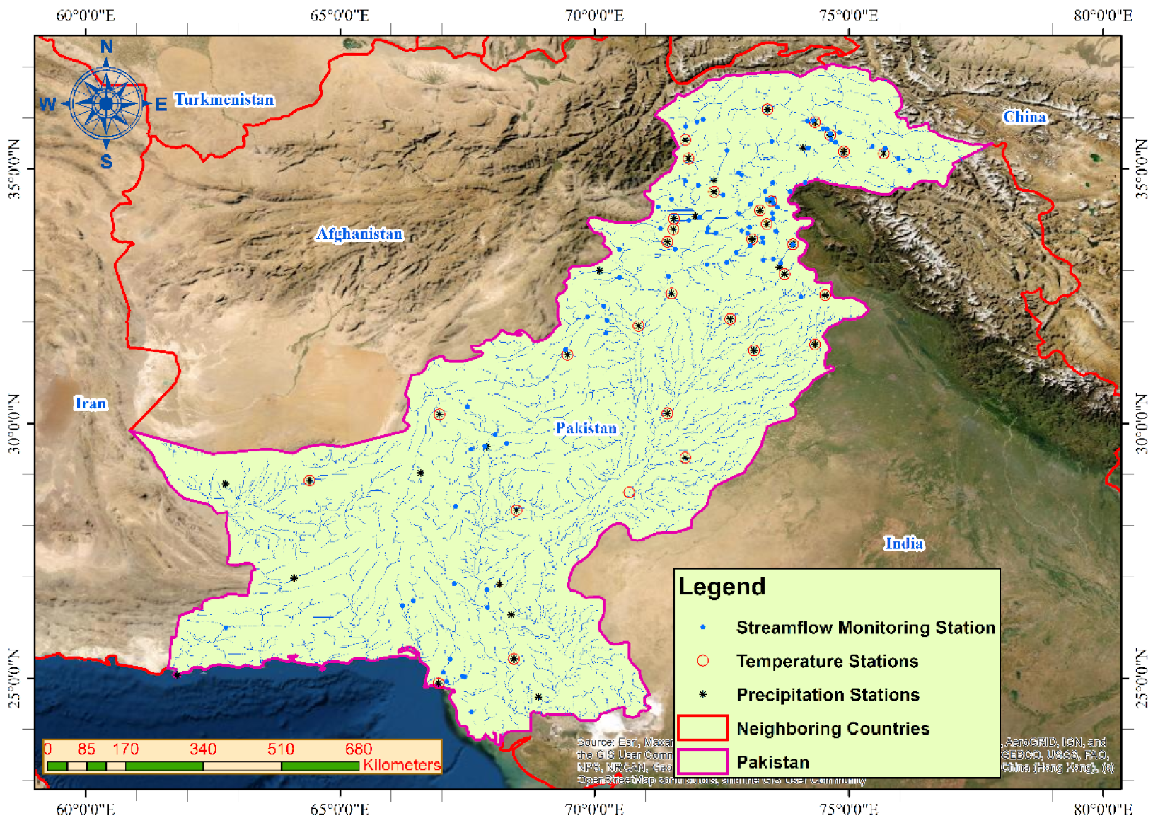
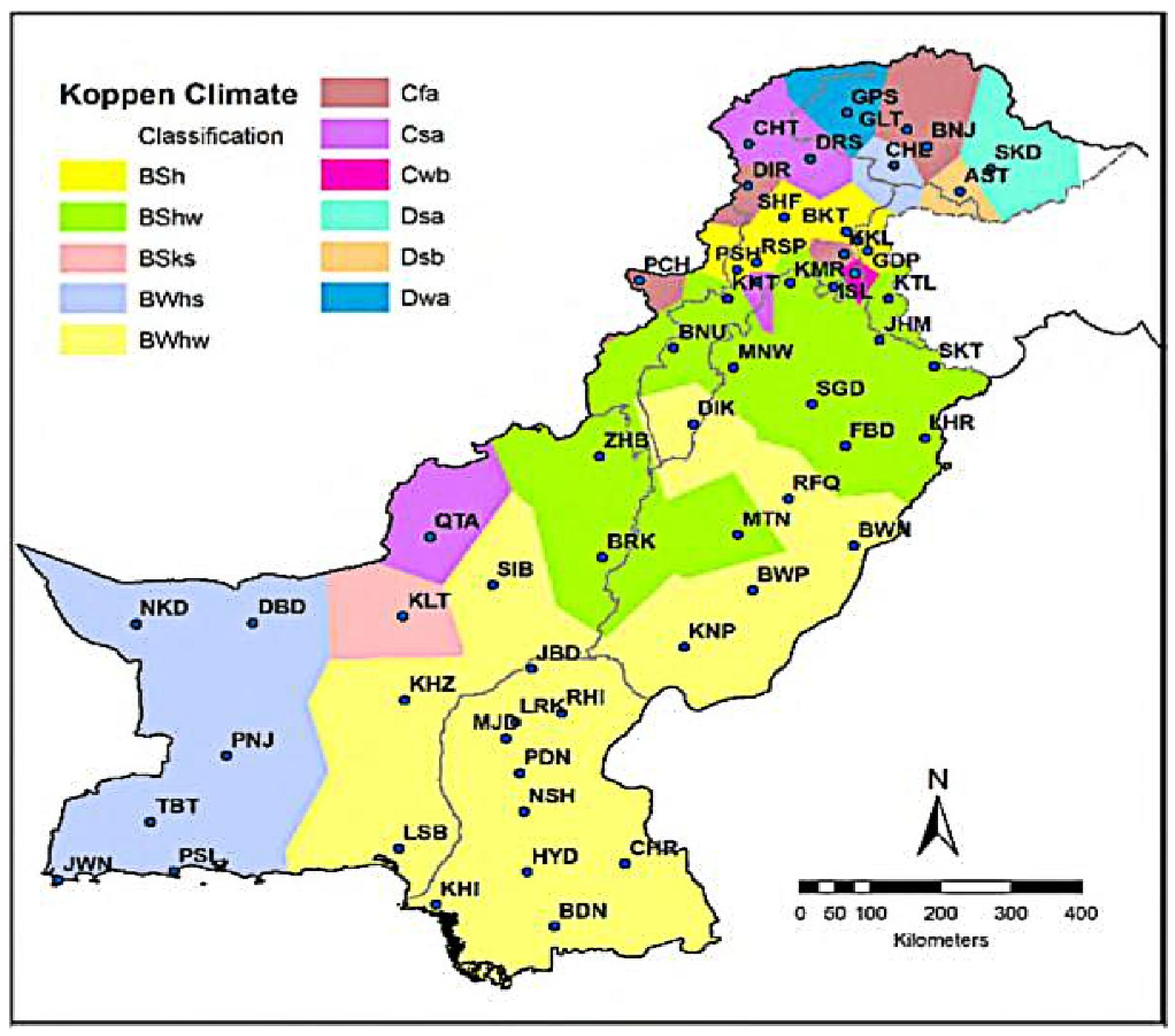
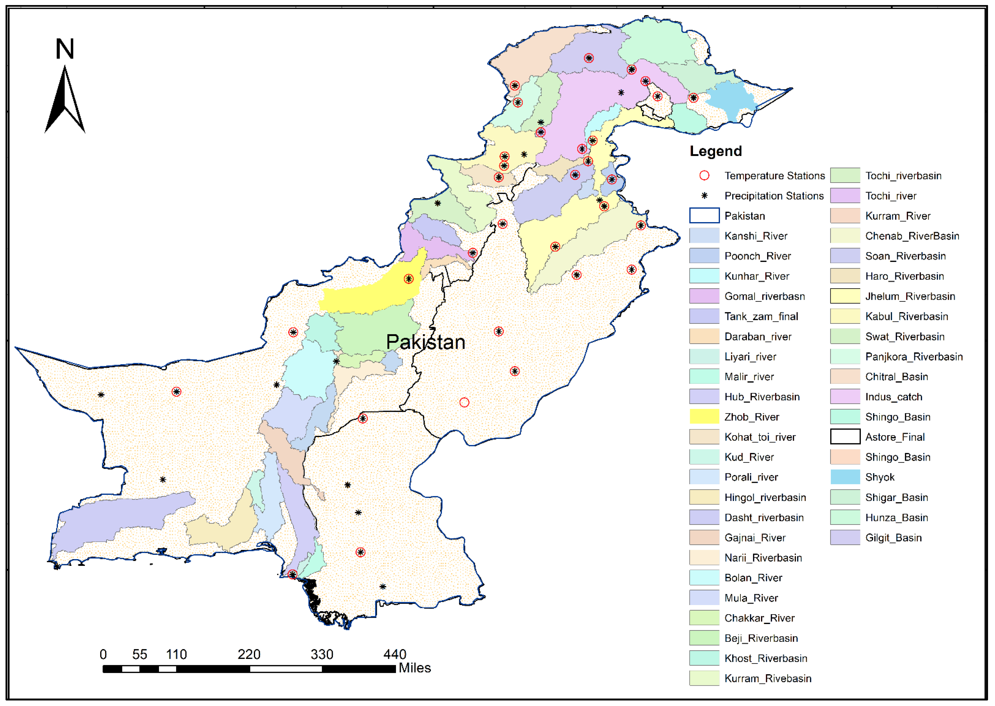
2.1. Study Area
2.2. Datasets Collection
2.3. Data Preparation
2.4. Data Uncertainty
2.5. Methods
2.5.1. NP (NP) Bivariate Model
2.5.2. Multivariate NP Analysis Model
2.5.3. Multivariate DL Analysis Model
3. Results
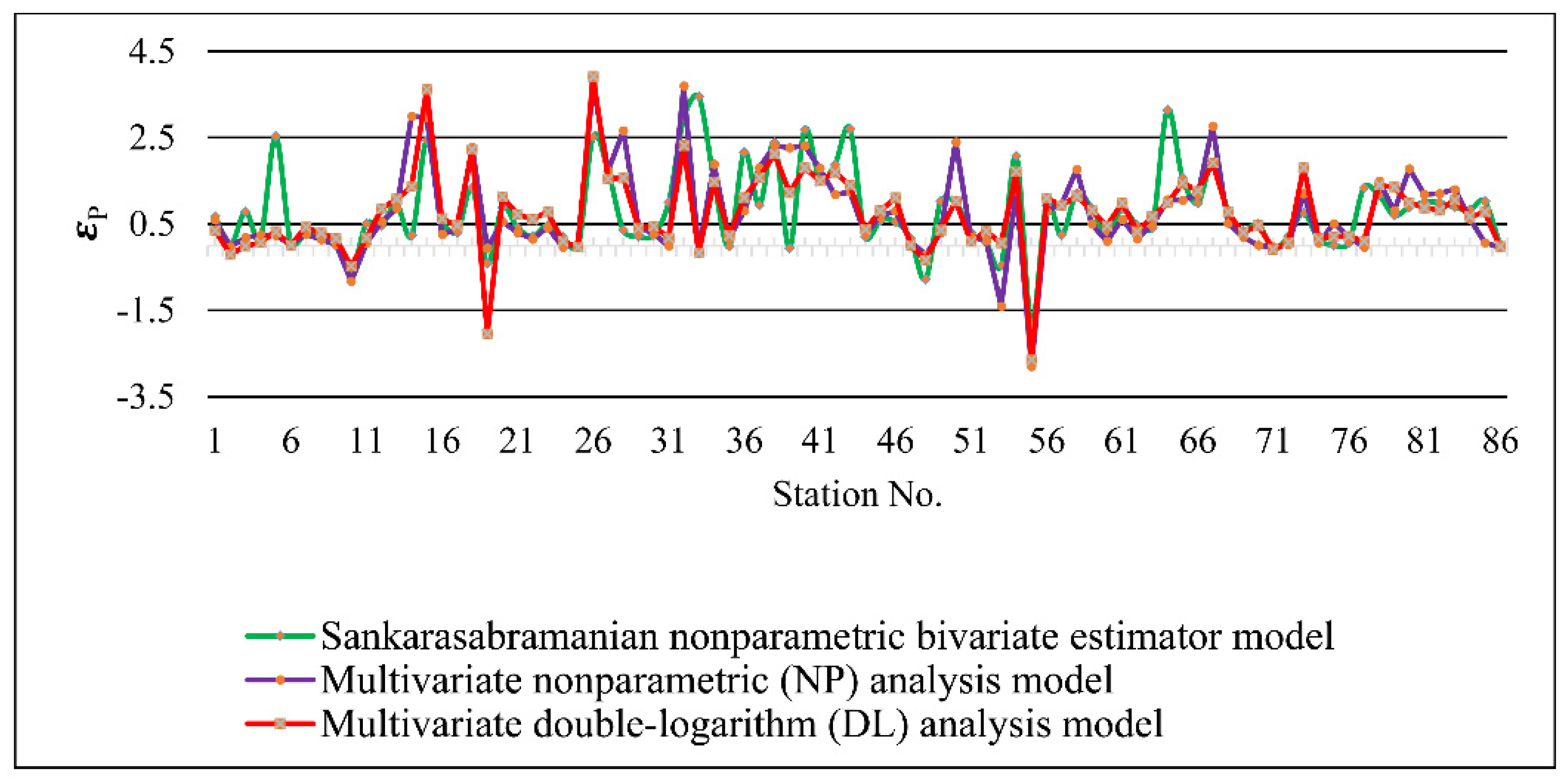
3.1. Precipitation Elasticity and Different Models
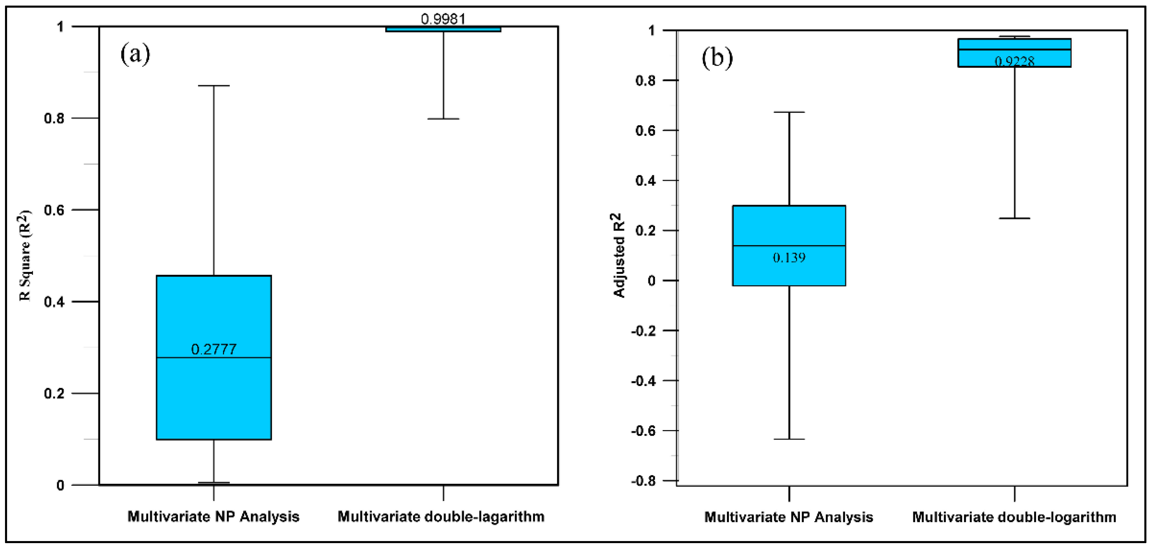
3.2. Comparison of Multivariate NP Analysis Model and Multivariate DL Model
3.3. Bivariate Versus Multivariate Analysis
3.4. Consequences of Instability Precipitation Elasticity
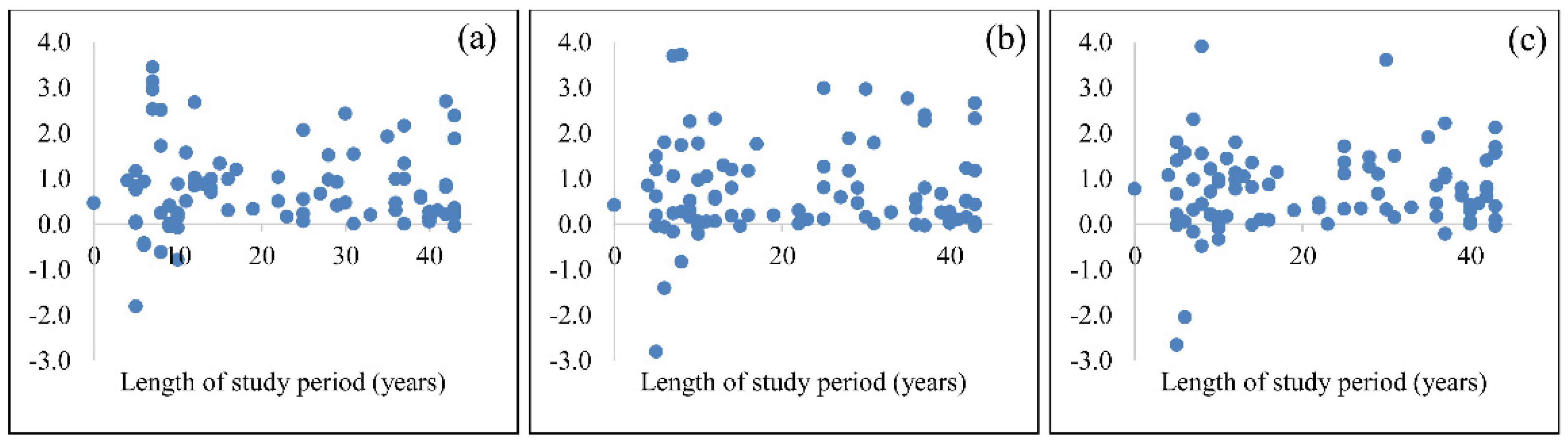
3.4.1. Precipitation Elasticity and Length of the Available Historical Record
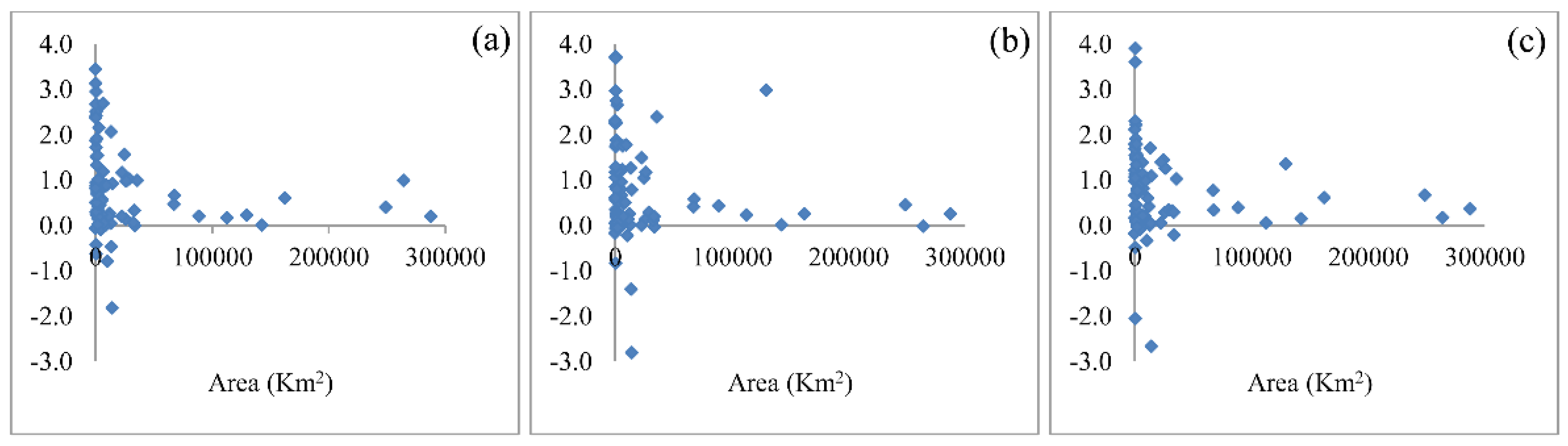
3.4.2. Precipitation Elasticity and Catchment Area
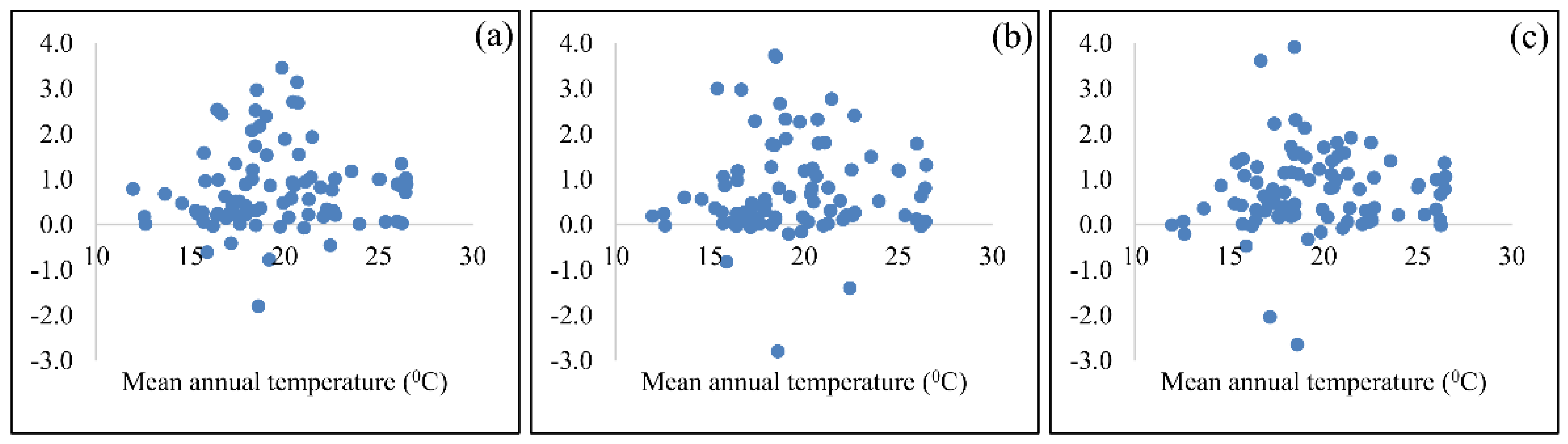
3.4.3. Precipitation Elasticity and Mean Annual Temperature
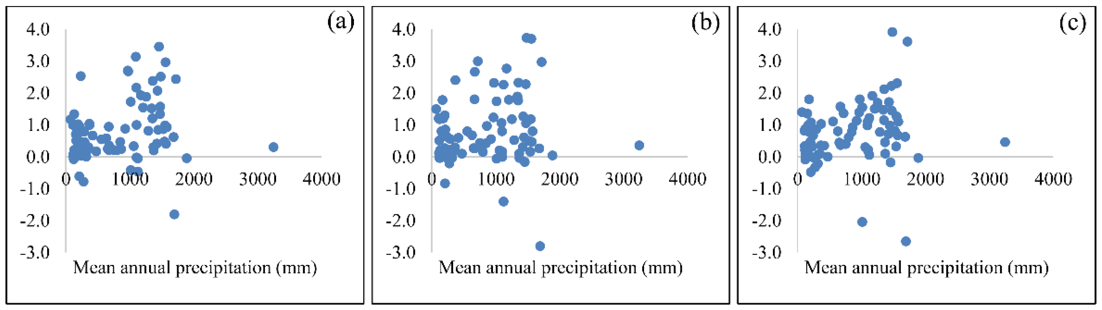
3.4.4. Precipitation Elasticity and Mean Annual Precipitation
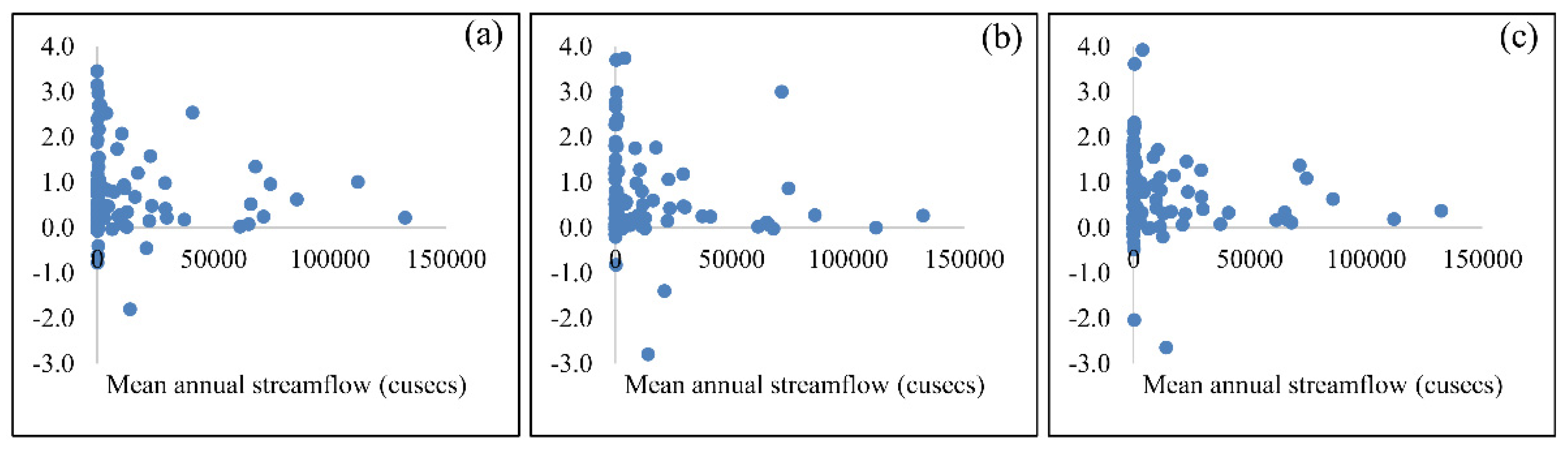
3.4.5. Precipitation Elasticity and Mean Annual Streamflow
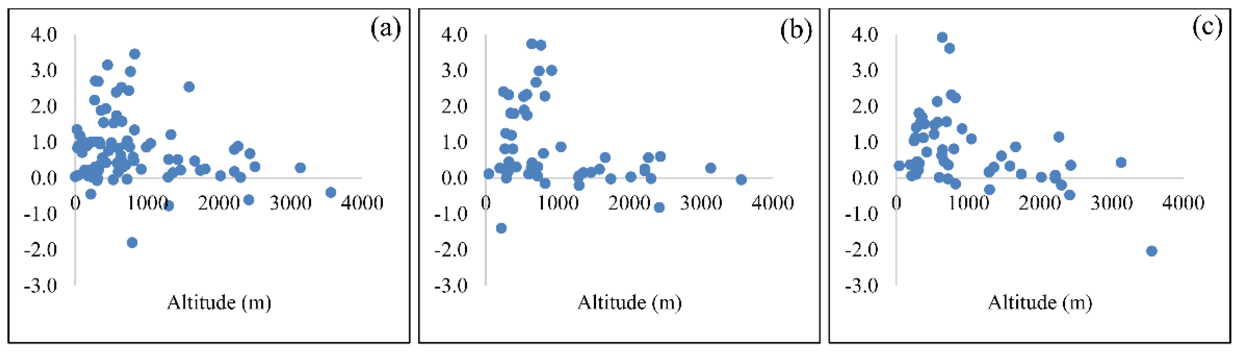
3.4.6. Precipitation Elasticity and Altitude
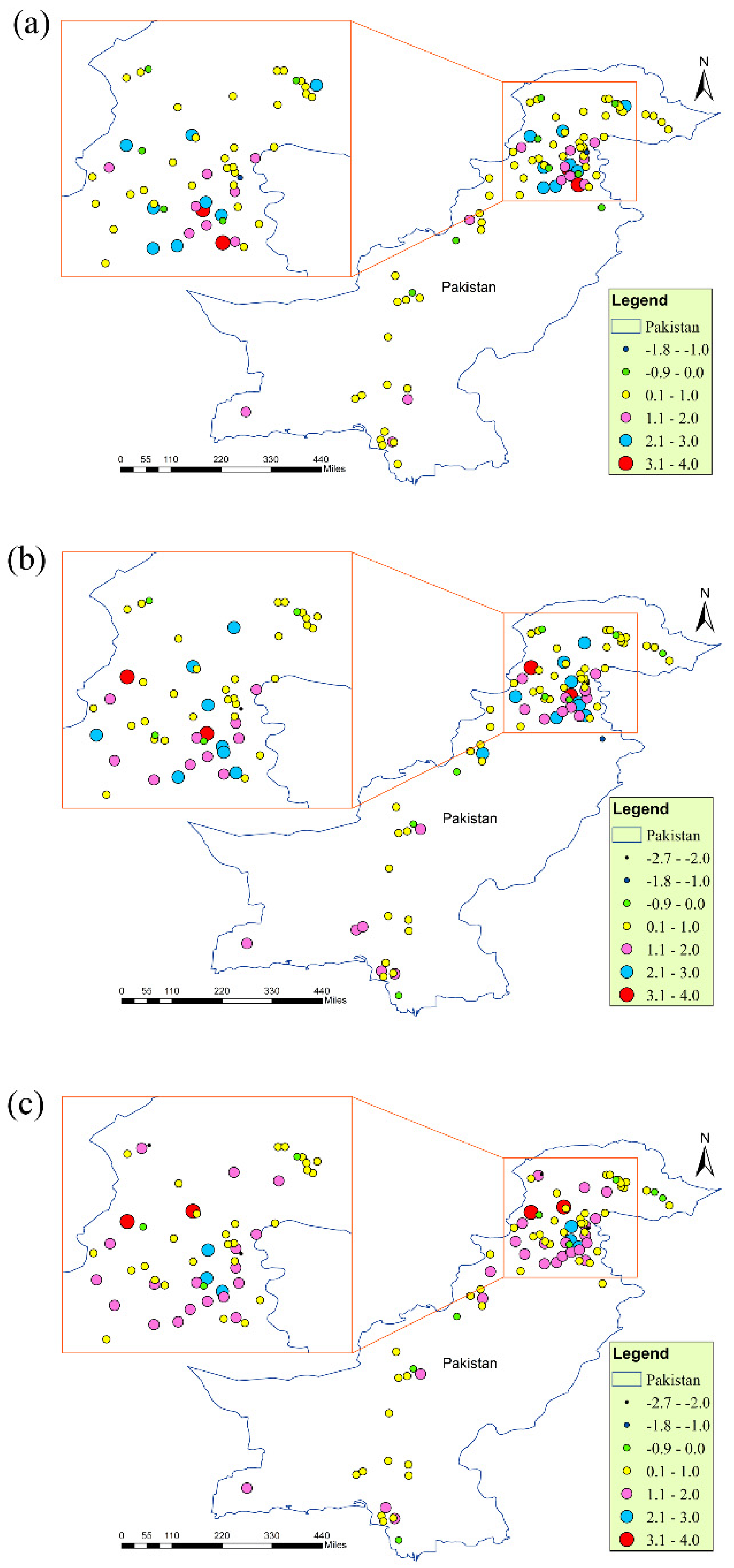
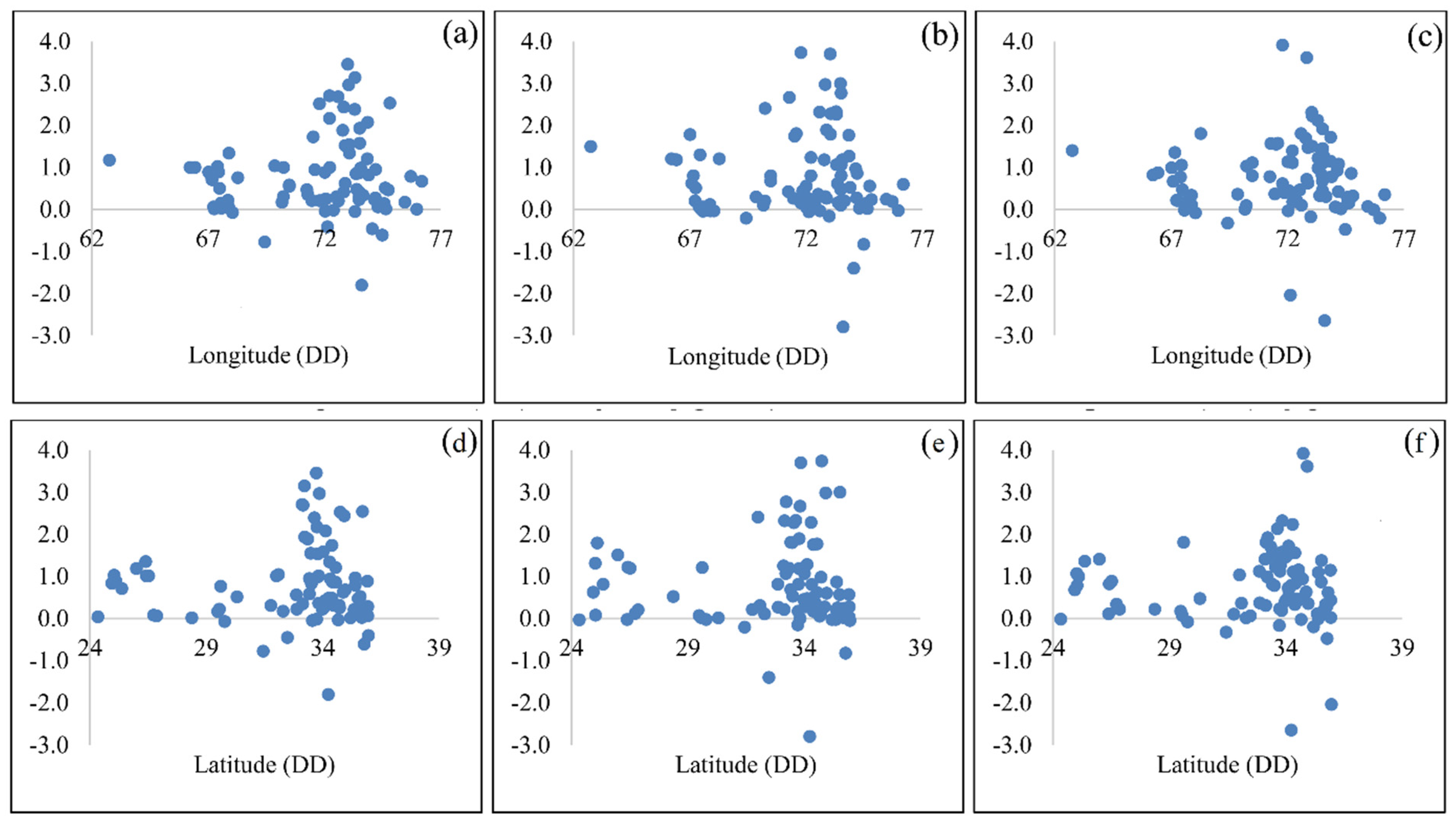
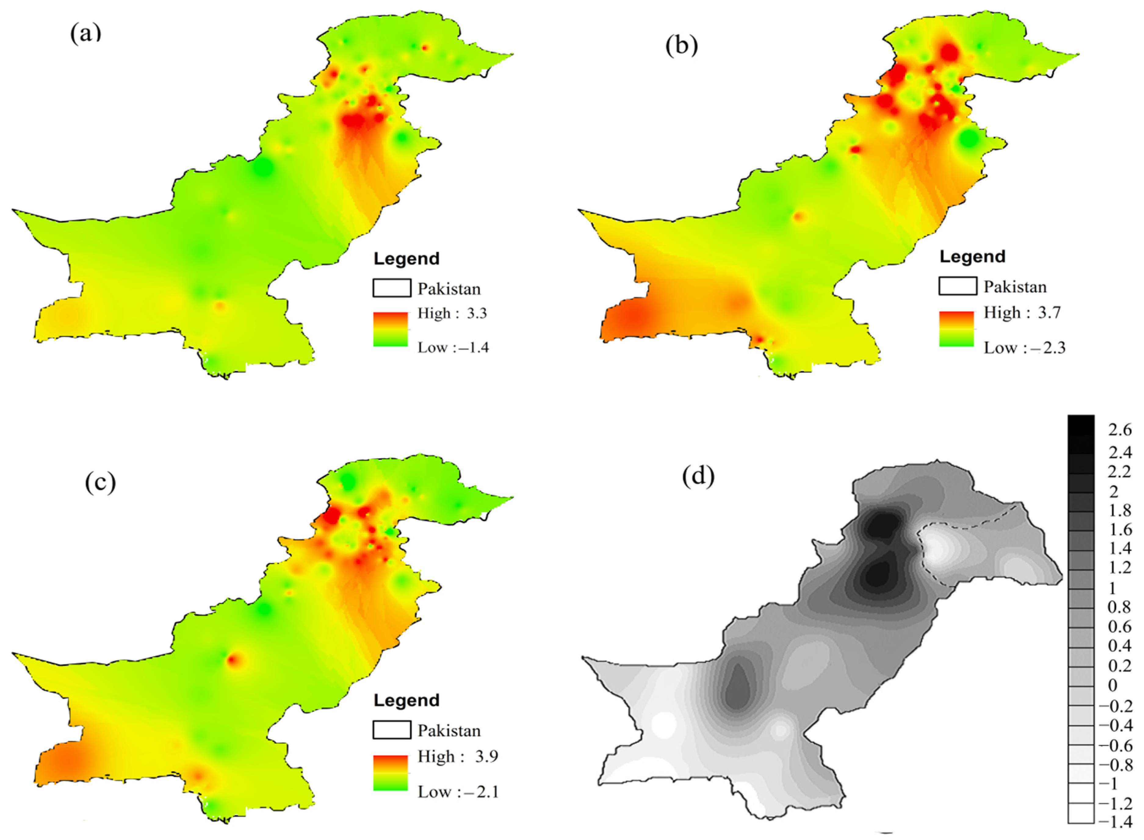
3.4.7. Precipitation Elasticity and Spatial Trends
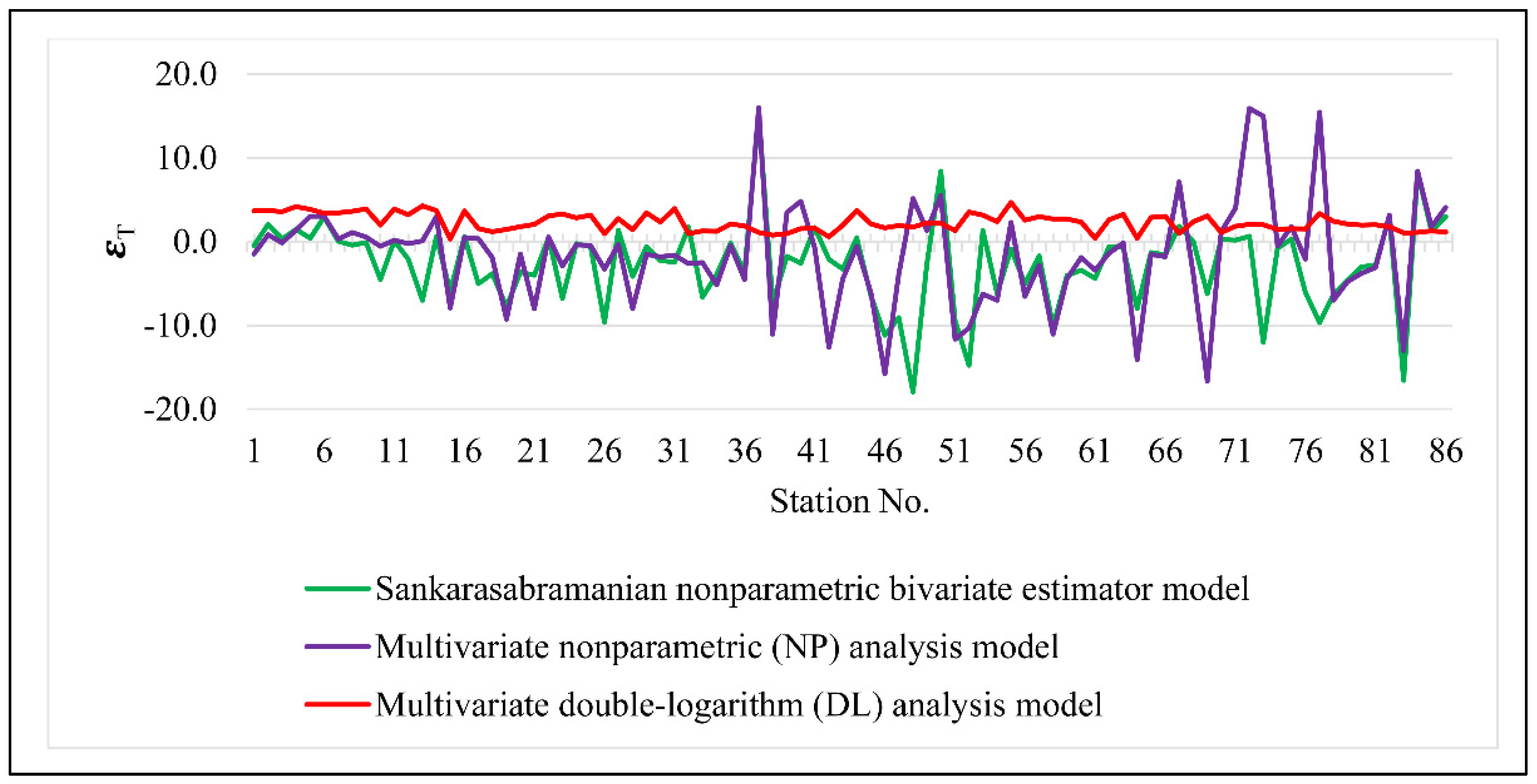
3.5. Temperature Elasticity
3.6. Recommendations Regarding Water Management and Policy-Making Based on Elasticity
4. Conclusions
Author Contributions
Funding
Institutional Review Board Statement
Informed Consent Statement
Data Availability Statement
Acknowledgments
Conflicts of Interest
Appendix A

| Station No. | River and Catchment Outlet Name | X Outlet DD | Y Outlet DD | Standard Elevation (m.a.s.l) | Available Record (yrs) | Catchment (km2) |
|---|---|---|---|---|---|---|
| 1 | Indus River at Kharmong | 76.1834 | 34.9728 | 2436 | 27 | 67,858 |
| 2 | Shyok River at Yugo | 75.9742 | 35.2050 | 2308 | 37 | 33,670 |
| 3 | Shigar River at Shigar | 75.7130 | 35.3993 | 2222 | 14 | 4144 |
| 4 | Indus River at Kachura | 75.4627 | 35.4449 | 2219 | 40 | 112,664 |
| 5 | Indus River near Gunji Bridge | 74.8102 | 35.7148 | 1591 | 7 | 785 |
| 6 | Hunza River at Dainyor Bridge | 74.2933 | 35.9458 | 2028 | 40 | 13,157 |
| 7 | Gilgit River at Gilgit | 74.1821 | 35.9452 | 3140 | 40 | 12,095 |
| 8 | Gilgit River at Alam Bridge | 74.5710 | 35.7816 | 1365 | 40 | 26,159 |
| 9 | Indus River at Partab Bridge | 74.6359 | 35.6913 | 1298 | 31 | 142,708 |
| 10 | Sai Nallah at Urkakai | 74.4870 | 35.7913 | 2421 | 8 | 554 |
| 11 | Indus River near Bunji Bridge | 74.6193 | 35.6102 | 1305 | 11 | 97 |
| 12 | Astore River at Doyian | 74.7380 | 35.5297 | 1668 | 36 | 4040 |
| 13 | Indus River at Raikot | 74.1948 | 35.4058 | 1052 | 4 | 385 |
| 14 | Indus River at Shatial Bridge | 73.4830 | 35.5409 | 922 | 25 | 129,499 |
| 15 | Gorbund River at Kabora | 72.8292 | 34.9242 | 749 | 30 | 635 |
| 16 | Indus River at Bisham Qila | 72.8902 | 34.8819 | 638 | 39 | 162,392 |
| 17 | Brandu River near Dagger | 72.5254 | 34.4902 | 669 | 36 | 598 |
| 18 | Siran River near Phulra | 73.0710 | 34.3079 | 829 | 37 | 1057 |
| 19 | Golan Gol River at Bubka | 72.1346 | 35.9687 | 3567 | 6 | 541 |
| 20 | Golan Gol River at Mastuj Bridge | 72.0148 | 35.9234 | 2270 | 12 | 518 |
| 21 | Siran River near Thapla | 72.8333 | 34.1229 | 430 | 9 | 2797 |
| 22 | Chitral River at Chitral | 71.7873 | 35.8339 | 1471 | 42 | 11,396 |
| 23 | Kabul River at Warsak | 71.2482 | 34.2581 | 650 | 9 | 67,340 |
| 24 | Swat River near Kalam | 72.6033 | 35.3647 | 1748 | 43 | 2020 |
| 25 | Swat River at Chakdara | 72.0369 | 34.6741 | 726 | 43 | 5776 |
| 26 | Panjkora River at Zulam Bridge | 71.7865 | 34.7594 | 645 | 8 | 597 |
| 27 | Swat River at Munda Dam | 71.5119 | 34.4079 | 580 | 8 | 392 |
| 28 | Bara River at Jhansi Post | 71.2955 | 33.8325 | 707 | 43 | 1847 |
| 29 | Kabul at Nowshehra | 71.8536 | 33.9839 | 328 | 43 | 88,578 |
| 30 | Kalpani River near Risalpur | 72.0654 | 34.0488 | 294 | 8 | 722 |
| 31 | Indus River at Khairabad/Mandori | 72.2286 | 33.8317 | 291 | 36 | 264,179 |
| 32 | Haro River at Dhartian | 73.0497 | 33.8574 | 773 | 7 | 621 |
| 33 | Nilan Kass River at Najaf Pur | 73.0037 | 33.7370 | 830 | 7 | 57 |
| 34 | Haro River near Khanpur | 72.8911 | 33.7899 | 539 | 28 | 777 |
| 35 | Haro River near Sanjawal | 72.3814 | 33.7483 | 313 | 9 | 1800 |
| 36 | Haro River at Gariala | 72.2168 | 33.7653 | 271 | 37 | 3056 |
| 37 | Kohat Toi at Jarma Weir | 71.5844 | 33.4278 | 350 | 6 | 1541 |
| 38 | Soan River at Chirah | 73.2995 | 33.6505 | 576 | 43 | 326 |
| 39 | Ling River near Kahuta | 73.3203 | 33.5603 | 533 | 9 | 153 |
| 40 | Soan at Gorakh Pur Bridge | 72.5949 | 33.1650 | 323 | 12 | 326 |
| 41 | Soan River near Rawalpindi | 73.0615 | 33.4915 | 399 | 31 | 1683 |
| 42 | Sil River near Chahan | 72.7874 | 33.3643 | 361 | 43 | 241 |
| 43 | Soan River at Dhok Pathan | 72.2099 | 33.1237 | 283 | 42 | 6475 |
| 44 | Indus River at Massan | 71.4547 | 32.8880 | 199 | 33 | 287,489 |
| 45 | Kurram River at Thal | 70.4857 | 33.4261 | 806 | 39 | 5543 |
| 46 | Tochi River at Tangi Post | 70.4930 | 32.8734 | 381 | 25 | 5128 |
| 47 | Tank Zam near Jandola | 70.1767 | 32.3073 | 604 | 23 | 2176 |
| 48 | Zhob River at Sherik Weir | 69.4283 | 31.4473 | 1304 | 10 | 10,360 |
| 49 | Gomal River at Khajurikach | 69.8628 | 32.1003 | 729 | 22 | 29,008 |
| 50 | Gomal River at Kot Murtaza | 70.2454 | 32.0227 | 252 | 37 | 36,001 |
| 51 | Daraban Zam at Zam Tower | 70.2295 | 31.7817 | 279 | 16 | 1062 |
| 52 | Indus River at Dadu Moro Bridge | 67.8856 | 26.7453 | 45 | 25 | 32,634 |
| 53 | Chenab River at Alexandria Bridge | 74.0584 | 32.4895 | 220 | 6 | 13,792 |
| 54 | Jhelum River at Chinari | 73.8580 | 34.1309 | 25 | 13,546 | |
| 55 | Jehlum at Majohi | 73.5958 | 34.2481 | 796 | 5 | 14,292 |
| 56 | Jhelum River at Domel | 73.5140 | 34.3296 | 714 | 29 | 14,504 |
| 57 | Neelum River at Dhundnial | 74.1367 | 34.7322 | 1815 | 10 | 5439 |
| 58 | Neelum at Nosheri | 73.8377 | 34.5566 | 1336 | 17 | 6809 |
| 59 | Kishanganga/Neelum at Muzaffarabad | 73.4854 | 34.4148 | 760 | 42 | 7278 |
| 60 | Kunhar River at Naran | 73.5003 | 34.7227 | 2508 | 41 | 1036 |
| 61 | Kunhar River at Talhata Bridge | 73.3540 | 34.5547 | 992 | 12 | 2354 |
| 62 | Kunhar River at Garhi Habibullah | 73.3873 | 34.3986 | 820 | 30 | 2383 |
| 63 | Jhelum River at Kohala | 73.4947 | 34.1295 | 586 | 29 | 248,898 |
| 64 | Bishan Daur Kas near Missa | 73.3203 | 33.2136 | 452 | 7 | 150 |
| 65 | Jehlum at Chattar Klass | 73.5119 | 34.0241 | 654 | 11 | 24,700 |
| 66 | Jhelum River at Azad Pattan | 73.5616 | 33.7828 | 506 | 28 | 26,485 |
| 67 | Kanshi River near Palote | 73.5156 | 33.2329 | 430 | 35 | 1111 |
| 68 | Poonch River near Kotli | 73.8967 | 33.5121 | 602 | 42 | 3237 |
| 69 | Jhelum River at Mangla Cableway | 73.6554 | 33.1480 | 335 | 19 | 33,411 |
| 70 | Khost River at Chappar Rift | 67.4999 | 30.3269 | 1431 | 22 | 1191 |
| 71 | Beji River at Babar Kach | 68.0450 | 29.7867 | 308 | 10 | 4558 |
| 72 | Nari River near Sibi | 67.8473 | 29.5587 | 134 | 10 | 22,559 |
| 73 | Chakkar River at Talli Tangi | 68.2746 | 29.6186 | 469 | 5 | 1484 |
| 74 | Bolan River at Kundlani Bridge | 67.5722 | 29.5004 | 188 | 10 | 4040 |
| 75 | Mula River at Naulang | 67.2708 | 28.3772 | 244 | 9 | 8599 |
| 76 | Gaj Nai near Jubble | 67.2420 | 26.8639 | 179 | 5 | 6863 |
| 77 | Indus River near Sehwan | 67.8971 | 26.3953 | 25 | 15 | 1250 |
| 78 | Dasht River at Mirani Dam Site | 62.7529 | 25.9970 | 68 | 5 | 22,533 |
| 79 | Hub River at Karpasaniwat | 67.1635 | 25.3759 | 96 | 14 | 1430 |
| 80 | Hub River at Bund Murad Khan | 67.0292 | 25.1167 | 47 | 10 | 9428 |
| 81 | Porali River at Sinchi Bent | 66.4370 | 26.5235 | 340 | 16 | 4040 |
| 82 | Kud River near Mai Gundrani | 66.2285 | 26.4235 | 232 | 14 | 2085 |
| 83 | Khadeji River at Super Highway | 67.4502 | 25.0300 | 170 | 13 | 567 |
| 84 | Liyari River at Super Highway Bridge | 67.0950 | 24.9397 | 33 | 5 | 207 |
| 85 | Malir River at Super Highway Bridge | 67.4045 | 25.0486 | 110 | 12 | 2235 |
| 86 | Malir River at National Highway | 67.5788 | 24.3406 | 2 | 5 | 2176 |
| S. No | Station Name | X (DD) | Y (DD) | Elevation (a.m.s.l) | Available Dataset |
|---|---|---|---|---|---|
| 1 | Astore | 74.9000 | 35.3333 | 2168.0 | Precipitation, temperature |
| 2 | Bunji | 74.6333 | 35.6667 | 1372.0 | Precipitation, temperature |
| 3 | Chillas | 74.1000 | 35.4167 | 1250 | Precipitation, temperature |
| 4 | Skardu (AP) | 75.6833 | 35.3000 | 2317.0 | Precipitation, temperature |
| 5 | Gilgit | 74.3333 | 35.9167 | 1460.0 | Precipitation, temperature |
| 6 | Dir | 71.8500 | 35.2000 | 1375.0 | Precipitation, temperature |
| 7 | Darosh | 71.7833 | 35.5667 | 1463.9 | Precipitation, temperature |
| 8 | Balakot | 72.3500 | 34.5500 | 995.4 | Precipitation, temperature |
| 9 | Cherat | 71.5500 | 33.8167 | 1372.0 | Precipitation, temperature |
| 10 | Dalbandin | 64.4000 | 28.8833 | 848.0 | Precipitation, temperature |
| 11 | D.I. Khan | 70.8667 | 31.9167 | 172.3 | Precipitation, temperature |
| 12 | Hyderabad | 68.4167 | 25.3833 | 28.0 | Precipitation, temperature |
| 13 | Jacobabad | 68.4667 | 28.3000 | 55.0 | Precipitation, temperature |
| 14 | Jhelum | 73.7333 | 32.9333 | 287.2 | Precipitation, temperature |
| 15 | Kakul | 73.2500 | 34.1833 | 1308.0 | Precipitation, temperature |
| 16 | Karachi (AP) | 66.9333 | 24.9000 | 22.0 | Precipitation, temperature |
| 17 | Kohat | 71.4330 | 33.5670 | 512.0 | Precipitation, temperature |
| 18 | Kotli | 73.9000 | 33.5167 | 614.0 | Precipitation, temperature |
| 19 | Muzaffarabad | 73.4833 | 34.3667 | 838.0 | Precipitation, temperature |
| 20 | Peshawar | 71.5600 | 33.87200 | 327.0 | Precipitation, temperature |
| 21 | Quetta | 66.9500 | 30.1833 | 1626.0 | Precipitation, temperature |
| 22 | Zhob | 69.4667 | 31.3500 | 1405.0 | Precipitation, temperature |
| 23 | Parachinar | 70.0833 | 33.8666 | 1725.0 | Precipitation, temperature |
| 24 | Bahawalpur | 71.7833 | 29.3333 | 110.0 | Precipitation, temperature |
| 25 | Bahawalnagar | 29.9500 | 68.9000 | 163.0 | Precipitation, temperature |
| 26 | Faisalabad | 73.1333 | 31.4333 | 185.6 | Precipitation, temperature |
| 27 | Gupis | 73.4000 | 36.1667 | 2156.0 | Precipitation, temperature |
| 28 | Islamabad | 73.1000 | 33.6170 | 508.0 | Precipitation, temperature |
| 29 | Khanpur | 70.6830 | 28.650 | 88.4 | Precipitation, temperature |
| 30 | Lahore (PBO) | 74.3333 | 31.5500 | 214.0 | Precipitation, temperature |
| 31 | Mianwali | 71.5170 | 32.5490 | 212.0 | Precipitation, temperature |
| 32 | Multan | 71.4333 | 30.2000 | 122.0 | Precipitation, temperature |
| 33 | Muree | 73.3830 | 33.9170 | 2213.0 | Precipitation, temperature |
| 34 | Sargodha | 72.6667 | 32.0500 | 187.0 | Precipitation, temperature |
| 35 | Sialkot | 74.5333 | 32.5167 | 255.1 | Precipitation, temperature |
| 36 | Mangla | 73.6333 | 33.0667 | 283.3 | Precipitation |
| 37 | Risalpur | 71.9830 | 34.067 | 317 | Precipitation |
| 38 | Saidu | 72.35 | 34.767 | 953 | Precipitation |
| 39 | Bannu | 70.1000 | 33.0000 | 406 | Precipitation |
| 40 | Paddian | 68.1333 | 26.8500 | 46 | Precipitation |
| 41 | Nawab Shah | 68.3667 | 26.2500 | 37 | Precipitation |
| 42 | Panjgur | 64.1000 | 26.9667 | 968 | Precipitation |
| 43 | Jiwani | 61.8000 | 25.0667 | 56 | Precipitation |
| 44 | Sibbi | 67.8833 | 29.5500 | 133 | Precipitation |
| 45 | Nokundi | 62.7500 | 28.8167 | 682 | Precipitation |
| 46 | Badin | 68.9000 | 24.6333 | 9 | Precipitation |
| 47 | Kalat | 66.5833 | 29.0333 | 2015 | Precipitation |
| Precipitation Elasticity | Temperature Elasticity | |||||||
|---|---|---|---|---|---|---|---|---|
| Catchment No. | River and Station Name | Available Record (Years) | Sankarasubramanian’s NP Bivariate Estimator | Multivariate NP Analysis | Multivariate DL Analysis | Sankarasubramanian’s NP Bivariate Estimator | Multivariate NP Analysis | Multivariate DL Analysis |
| 1 | Indus River at Kharmong | 27 | 0.7 | 0.6 | 0.3 | −0.5 | −1.5 | 3.7 |
| 2 | Shyok River at Yugo | 37 | 0.0 | 0.0 | −0.2 | 2.1 | 0.8 | 3.7 |
| 3 | Shigar River at Shigar | 14 | 0.8 | 0.2 | 0.0 | 0.3 | −0.2 | 3.6 |
| 4 | Indus River at Kachura | 40 | 0.2 | 0.2 | 0.1 | 1.5 | 1.4 | 4.2 |
| 5 | Indus River near Gunji Bridge | 7 | 2.5 | 0.2 | 0.3 | 0.4 | 3.0 | 3.8 |
| 6 | Hunza River at Dainyor Bridge | 40 | 0.1 | 0.0 | 0.0 | 2.9 | 3.0 | 3.4 |
| 7 | Gilgit River at Gilgit | 40 | 0.3 | 0.3 | 0.4 | 0.0 | 0.3 | 3.4 |
| 8 | Gilgit River at Alam Bridge | 40 | 0.1 | 0.1 | 0.3 | −0.4 | 1.1 | 3.6 |
| 9 | Indus River at Partab Bridge | 31 | 0.0 | 0.0 | 0.2 | −0.1 | 0.5 | 3.9 |
| 10 | Sai Nallah at Urkakai | 8 | −0.6 | −0.8 | −0.5 | −4.5 | −0.5 | 2.0 |
| 11 | Indus River near Bunji Bridge | 11 | 0.5 | 0.1 | 0.2 | 0.1 | 0.2 | 3.9 |
| 12 | Astore River at Doyian | 36 | 0.5 | 0.6 | 0.9 | −2.1 | −0.2 | 3.2 |
| 13 | Indus River at Raikot | 4 | 1.0 | 0.9 | 1.1 | −7.0 | 0.1 | 4.3 |
| 14 | Indus River at Shatial Bridge | 25 | 0.2 | 3.0 | 1.4 | 0.6 | 3.0 | 3.7 |
| 15 | Gorbund River at Kabora | 30 | 2.4 | 3.0 | 3.6 | −5.9 | −7.9 | 0.3 |
| 16 | Indus River at Bisham Qila | 39 | 0.6 | 0.3 | 0.6 | 0.6 | 0.5 | 3.7 |
| 17 | Brandu River near Dagger | 36 | 0.3 | 0.4 | 0.5 | −5.0 | 0.4 | 1.6 |
| 18 | Siran River near Phulra | 37 | 1.3 | 2.3 | 2.2 | −3.8 | −1.9 | 1.2 |
| 19 | Golan Gol River at Bubka | 6 | −0.4 | −0.1 | −2.0 | −7.8 | −9.3 | 1.5 |
| 20 | Golan Gol River at Mastuj Bridge | 12 | 0.9 | 0.6 | 1.1 | −3.7 | −1.5 | 1.8 |
| 21 | Siran River near Thapla | 9 | 0.4 | 0.3 | 0.7 | −4.0 | −8.0 | 2.1 |
| 22 | Chitral River at Chitral | 42 | 0.2 | 0.1 | 0.6 | 0.4 | 0.6 | 3.1 |
| 23 | Kabul River at Warsak | 9 | 0.5 | 0.4 | 0.8 | −6.8 | −2.9 | 3.3 |
| 24 | Swat River near Kalam | 43 | 0.2 | 0.0 | 0.1 | −0.2 | −0.4 | 2.8 |
| 25 | Swat River at Chakdara | 43 | 0.0 | 0.0 | 0.0 | −0.6 | −0.5 | 3.2 |
| 26 | Panjkora River at Zulam Bridge | 8 | 2.5 | 3.7 | 3.9 | −9.6 | −3.3 | 1.0 |
| 27 | Swat River at Munda Dam | 8 | 1.7 | 1.7 | 1.5 | 1.4 | −0.3 | 2.8 |
| 28 | Bara River at Jhansi Post | 43 | 0.4 | 2.7 | 1.6 | −4.1 | −8.0 | 1.4 |
| 29 | Kabul at Nowshehra | 43 | 0.2 | 0.4 | 0.4 | −0.6 | −1.5 | 3.5 |
| 30 | Kalpani River near Risalpur | 8 | 0.2 | 0.3 | 0.4 | −2.3 | −1.8 | 2.4 |
| 31 | Indus River at Khairabad/Mandori | 36 | 1.0 | 0.0 | 0.2 | −2.5 | −1.6 | 3.9 |
| 32 | Haro River at Dhartian | 7 | 3.0 | 3.7 | 2.3 | 1.7 | −2.6 | 1.0 |
| 33 | Nilan Kass River at Najaf Pur | 7 | 3.5 | −0.2 | −0.2 | −6.6 | −2.5 | 1.3 |
| 34 | Haro River near Khanpur | 28 | 1.5 | 1.9 | 1.5 | −3.9 | −5.2 | 1.2 |
| 35 | Haro River near Sanjawal | 9 | 0.0 | 0.2 | 0.2 | −0.2 | −0.5 | 2.1 |
| 36 | Haro River at Gariala | 37 | 2.2 | 0.8 | 1.1 | −3.6 | −4.5 | 1.9 |
| 37 | Kohat Toi at Jarma Weir | 6 | 0.9 | 1.8 | 1.6 | 15.3 | 16.0 | 1.1 |
| 38 | Soan River at Chirah | 43 | 2.4 | 2.3 | 2.1 | −7.3 | −11.1 | 0.8 |
| 39 | Ling River near Kahuta | 9 | −0.1 | 2.3 | 1.2 | −1.8 | 3.5 | 0.9 |
| 40 | Soan at Gorakh Pur Bridge | 12 | 2.7 | 2.3 | 1.8 | −2.6 | 4.8 | 1.6 |
| 41 | Soan River near Rawalpindi | 31 | 1.5 | 1.8 | 1.5 | 1.7 | −0.7 | 1.6 |
| 42 | Sil River near Chahan | 43 | 1.9 | 1.2 | 1.7 | −2.1 | −12.6 | 0.6 |
| 43 | Soan River at Dhok Pathan | 42 | 2.7 | 1.2 | 1.4 | −3.3 | −4.4 | 2.0 |
| 44 | Indus River at Massan | 33 | 0.2 | 0.3 | 0.4 | 0.4 | −0.6 | 3.7 |
| 45 | Kurram River at Thal | 39 | 0.6 | 0.7 | 0.8 | −6.5 | −6.2 | 2.1 |
| 46 | Tochi River at Tangi Post | 25 | 0.6 | 0.8 | 1.1 | −11.2 | −15.8 | 1.6 |
| 47 | Tank Zam near Jandola | 23 | 0.2 | 0.1 | 0.0 | −9.1 | −3.9 | 1.9 |
| 48 | Zhob River at Sherik Weir | 10 | −0.8 | −0.2 | −0.3 | −17.9 | 5.1 | 1.8 |
| 49 | Gomal River at Khajurikach | 22 | 1.0 | 0.3 | 0.4 | −2.7 | 1.3 | 2.3 |
| 50 | Gomal River at Kot Murtaza | 37 | 1.0 | 2.4 | 1.0 | 8.4 | 5.5 | 2.2 |
| 51 | Daraban Zam at Zam Tower | 16 | 0.3 | 0.2 | 0.1 | −9.5 | −11.6 | 1.3 |
| 52 | Indus River at Dadu Moro Bridge | 25 | 0.1 | 0.1 | 0.3 | −14.8 | −10.3 | 3.5 |
| 53 | Chenab River at Alexandria Bridge | 6 | −0.5 | −1.4 | 0.1 | 1.3 | −6.3 | 3.2 |
| 54 | Jhelum River at Chinari | 25 | 2.1 | 1.3 | 1.7 | −6.2 | −7.0 | 2.4 |
| 55 | Jehlum at Majohi | 5 | −1.8 | −2.8 | −2.7 | −0.9 | 2.3 | 4.7 |
| 56 | Jhelum River at Domel | 29 | 0.9 | 0.8 | 1.1 | −5.0 | −6.5 | 2.6 |
| 57 | Neelum River at Dhundnial | 10 | 0.2 | 1.0 | 0.9 | −1.7 | −2.8 | 3.0 |
| 58 | Neelum at Nosheri | 17 | 1.2 | 1.8 | 1.1 | −10.1 | −11.0 | 2.7 |
| 59 | Kishanganga/Neelum at Muzaffarabad | 42 | 0.9 | 0.5 | 0.8 | −4.1 | −4.4 | 2.7 |
| 60 | Kunhar River at Naran | 41 | 0.3 | 0.1 | 0.5 | −3.4 | −1.9 | 2.3 |
| 61 | Kunhar River at Talhata Bridge | 12 | 0.8 | 0.6 | 1.0 | −4.4 | −3.4 | 0.4 |
| 62 | Kunhar River at Garhi Habibullah | 30 | 0.5 | 0.2 | 0.3 | −0.6 | −1.4 | 2.6 |
| 63 | Jhelum River at Kohala | 29 | 0.4 | 0.5 | 0.7 | −0.7 | −0.1 | 3.3 |
| 64 | Bishan Daur Kas near Missa | 7 | 3.1 | 1.1 | 1.0 | −8.0 | −14.1 | 0.4 |
| 65 | Jehlum at Chattar Klass | 11 | 1.6 | 1.1 | 1.4 | −1.3 | −1.5 | 2.9 |
| 66 | Jhelum River at Azad Pattan | 28 | 1.0 | 1.2 | 1.3 | −1.6 | −1.8 | 3.0 |
| 67 | Kanshi River near Palote | 35 | 1.9 | 2.8 | 1.9 | 1.8 | 7.1 | 1.0 |
| 68 | Poonch River near Kotli | 42 | 0.8 | 0.5 | 0.8 | 0.0 | −4.0 | 2.4 |
| 69 | Jhelum River at Mangla Cableway | 19 | 0.3 | 0.2 | 0.3 | −6.2 | −16.6 | 3.1 |
| 70 | Khost River at Chappar Rift | 22 | 0.5 | 0.0 | 0.5 | 0.3 | 1.2 | 1.1 |
| 71 | Beji River at Babar Kach | 10 | −0.1 | 0.0 | −0.1 | 0.2 | 4.0 | 1.8 |
| 72 | Nari River near Sibi | 10 | 0.2 | 0.0 | 0.1 | 0.6 | 15.9 | 2.0 |
| 73 | Chakkar River at Talli Tangi | 5 | 0.8 | 1.2 | 1.8 | −12.0 | 15.0 | 2.0 |
| 74 | Bolan River at Kundlani Bridge | 10 | 0.2 | 0.1 | 0.2 | −0.8 | −0.5 | 1.5 |
| 75 | Mula River at Naulang | 9 | 0.0 | 0.5 | 0.2 | 0.3 | 1.8 | 1.5 |
| 76 | Gaj Nai near Jubble | 5 | 0.1 | 0.2 | 0.2 | −6.0 | −2.1 | 1.5 |
| 77 | Indus River near Sehwan | 15 | 1.3 | 0.0 | 0.1 | −9.7 | 15.4 | 3.3 |
| 78 | Dasht River at Mirani Dam Site | 5 | 1.2 | 1.5 | 1.4 | −6.3 | −7.0 | 2.4 |
| 79 | Hub River at Karpasaniwat | 14 | 0.7 | 0.8 | 1.3 | −4.6 | −4.8 | 2.1 |
| 80 | Hub River at Bund Murad Khan | 10 | 0.9 | 1.8 | 1.0 | −3.0 | −3.8 | 2.0 |
| 81 | Porali River at Sinchi Bent | 16 | 1.0 | 1.2 | 0.9 | −2.8 | −3.1 | 2.0 |
| 82 | Kud River near Mai Gundrani | 14 | 1.0 | 1.2 | 0.8 | 3.0 | 3.2 | 1.8 |
| 83 | Khadeji River at Super Highway | 13 | 0.9 | 1.3 | 1.1 | −16.6 | −13.0 | 1.1 |
| 84 | Liyari River at Super Highway Bridge | 5 | 0.8 | 0.6 | 0.7 | 8.3 | 8.4 | 1.1 |
| 85 | Malir River at Super Highway Bridge | 12 | 1.0 | 0.1 | 0.8 | 1.3 | 1.8 | 1.3 |
| 86 | Malir River at National Highway | 5 | 0.0 | 0.0 | 0.0 | 3.0 | 4.1 | 1.1 |

References
- IPCC, 2018: Global Warming of 1.5 °C. An IPCC Special Report on the Impacts of Global Warming of 1.5 °C above Pre-Industrial Levels and Related Global Greenhouse Gas Emission Pathways, in the Context of Strengthening the Global Response to the Threat of Climate Change, Sustainable Development, and Efforts to Eradicate Poverty. Available online: https://www.ipcc.ch/site/assets/uploads/sites/2/2019/06/SR15_Full_Report_Low_Res.pdf (accessed on 13 February 2022).
- Heikkila, E.J.; Huang, M. Adaptation to flooding in urban areas: An economic primer. Public Works Manag. Policy 2014, 19, 11–36. [Google Scholar] [CrossRef]
- Hassol, S.J.; Torok, S.; Lewis, S.; Luganda, P. Unnatural Disasters: Communicating Linkages Between Extreme Events and Climate Change; World Meteorological Organization (WMO): Geneva, Switzerland, 2017. [Google Scholar]
- Chu, J.T.; Xia, J.; Xu, C.-Y.; Singh, V.P. Statistical downscaling of daily mean temperature, pan evaporation and precipitation for climate change scenarios in Haihe River, China. Theor. Appl. Climatol. 2010, 99, 149–161. [Google Scholar] [CrossRef]
- Khattak, M.S.; Babel, M.S.; Sharif, M. Hydro-meteorological trends in the upper Indus River basin in Pakistan. Clim. Res. 2011, 46, 103–119. [Google Scholar] [CrossRef]
- Wang, J.; Ishidaira, H.; Xu, Z.X. Effects of climate change and human activities on inflow into the Hoabinh Reservoir in the Red River basin. Procedia Environ. Sci. 2012, 13, 1688–1698. [Google Scholar] [CrossRef] [Green Version]
- Pandey, V.P.; Shrestha, D.; Adhikari, M.; Shakya, S. Streamflow alterations, attributions, and implications in extended east Rapti watershed, central-southern Nepal. Sustainability 2020, 12, 3829. [Google Scholar] [CrossRef]
- Gemmer, M.; Becker, S.; Jiang, T. Detection and Visualisation of Climate Trends in China; Diskussionsbeiträge; Zentrum für Internationale Entwicklungs-und Umweltforschung: Kiel, Germany, 2003. [Google Scholar]
- Zhang, Q.; Jiang, T.; Gemmer, M.; Becker, S. Precipitation, temperature and runoff analysis from 1950 to 2002 in the Yangtze basin, China/Analyse des précipitations, températures et débits de 1950 à 2002 dans le bassin du Yangtze, en Chine. Hydrol. Sci. J. 2005, 50, 66–80. [Google Scholar] [CrossRef] [Green Version]
- Singh, P.; Kumar, V.; Thomas, T.; Arora, M. Basin-wide assessment of temperature trends in northwest and central India. Hydrol. Sci. J. 2008, 53, 421–433. [Google Scholar] [CrossRef]
- Huang, Y.; Cai, J.; Yin, H.; Cai, M. Correlation of precipitation to temperature variation in the Huanghe River (Yellow River) basin during 1957–2006. J. Hydrol. 2009, 372, 1–8. [Google Scholar] [CrossRef]
- Iqbal, M.S.; Dahri, Z.H.; Querner, E.P.; Khan, A. Impact of Climate Change on Flood Frequency and Intensity in the Kabul River Basin. Geosciences 2018, 5, 114. [Google Scholar] [CrossRef] [Green Version]
- Ahmad, I.; Tang, D.; Wang, T.; Wang, M.; Wagan, B. Precipitation trends over time using Mann-Kendall and spearman’s rho tests in swat river basin, Pakistan. Adv. Meteorol. 2015, 2015, 431860. [Google Scholar] [CrossRef] [Green Version]
- Shukla, P.R.; Skea, J.; Calvo Buendia, E.; Masson-Delmotte, V.; Pörtner, H.-O.; Roberts, D.C.; Zhai, P.; Slade, R.; Connors, S.; Van Diemen, R.; et al. IPCC, 2019: Climate Change and Land: An IPCC special report on climate change, desertification, land degradation, sustainable land management, food security, and greenhouse gas fluxes in terrestrial ecosystems. In Intergovernmental Panel on Climate Change (IPCC); United Nations: Geneva, Switzerland, 2019. [Google Scholar] [CrossRef]
- Zommers, Z.; van der Geest, K.; De Sherbinin, A.; Kienberger, S.; Roberts, E.; Harootunian, G.; Sitati, A.; James, R. Loss and Damage: The Role of Ecosystem Services; United Nations Environment Programme: Nairobi, Kenya, 2016; p. 84. [Google Scholar]
- The Institute for Economics and Peace. Global Peace Index 2017—Measuring Peace in a Complex World; The Institute for Economics and Peace: Sydney, Australia, 2018; Volume 1, pp. 1–140. [Google Scholar]
- Eckstein, D.; Künzel, V.; Schäfer, L.; Winges, M. Global Climate Risk Index 2020; Germanwatch: Bonn, Germany, 2019; Volume 1, pp. 1–44. [Google Scholar]
- Rehman, A.; Jingdong, L.; Shahzad, B.; Chandio, A.A.; Hussain, I.; Nabi, G.; Iqbal, M.S. Economic perspectives of major field crops of Pakistan: An empirical study. Pac. Sci. Rev. B Humanit. Soc. Sci. 2015, 1, 145–158. [Google Scholar] [CrossRef] [Green Version]
- Ramachandran, V.; Ramalakshmi, R.; Kavin, B.P.; Hussain, I.; Almaliki, A.H.; Almaliki, A.A.; Elnaggar, A.Y.; Hussein, E.E. Exploiting IoT and Its Enabled Technologies for Irrigation Needs in Agriculture. Water 2022, 14, 719. [Google Scholar] [CrossRef]
- Talchabhadel, R.; Aryal, A.; Kawaike, K.; Yamanoi, K.; Nakagawa, H.; Bhatta, B.; Karki, S.; Thapa, B.R. Evaluation of precipitation elasticity using precipitation data from ground and satellite-based estimates and watershed modeling in Western Nepal. J. Hydrol. Reg. Stud. 2021, 33, 100768. [Google Scholar] [CrossRef]
- Vano, J.A.; Das, T.; Lettenmaier, D.P. Hydrologic sensitivities of Colorado River runoff to changes in precipitation and temperature. J. Hydrometeorol. 2012, 13, 932–949. [Google Scholar] [CrossRef] [Green Version]
- Zuo, D.; Xu, Z.; Wu, W.; Zhao, J.; Zhao, F. Identification of streamflow response to climate change and human activities in the wei river Basin, China. Water Resour. Manag. 2014, 28, 833–851. [Google Scholar] [CrossRef]
- Sun, S.; Chen, H.; Ju, W.; Song, J.; Zhang, H.; Sun, J.; Fang, Y. Effects of climate change on annual streamflow using climate elasticity in Poyang Lake Basin, China. Theor. Appl. Climatol. 2013, 112, 169–183. [Google Scholar] [CrossRef]
- Junior, D.S.R.; Cerqueira, C.M.; Vieira, R.F.; Martins, E.S. Budyko’s Framework and Climate Elasticity Concept in the Estimation of Climate Change Impacts on the Long-Term Mean Annual Streamflow. World Environ. Water Resour. Congr. 2013, 2013, 1110–1120. [Google Scholar] [CrossRef]
- Frederick, K.D.; Major, D.C. Climate Change and Water Resources. Clim. Chang. 1997, 37, 7–23. [Google Scholar] [CrossRef]
- Nash, L.L.; Gleick, P.H. Sensitivity of streamflow in the Colorado basin to climatic changes. J. Hydrol. 1991, 125, 221–241. [Google Scholar] [CrossRef]
- Jeton, A.E.; Dettinger, M.D.; Smith, J.L. Potential effects of climate change on streamflow, eastern and western slopes of the Sierra Nevada, California and Nevada. Water Resour. Investig. Rep. 1996, 95, 4260. [Google Scholar]
- Sankarasubramanian, A.; Vogel, R.M.; Limbrunner, J.F. Climate elasticity of streamflow in the United States. Water Resour. Res. 2001, 37, 1771–1781. [Google Scholar] [CrossRef]
- Jones, R.N.; Chiew, F.H.S.; Boughton, W.C.; Zhang, L. Estimating the sensitivity of mean annual runoff to climate change using selected hydrological models. Adv. Water Resour. 2006, 29, 1419–1429. [Google Scholar] [CrossRef] [Green Version]
- Karki, M.B.; Shrestha, A.B.; Winiger, M. Enhancing Knowledge Management and Adaptation Capacity for Integrated Management of Water Resources in the Indus River Basin. Mt. Res. Dev. 2011, 31, 242–251. [Google Scholar] [CrossRef]
- Khan, A.; Richards, K.; Mcrobie, F.A.; Booij, M.J. Impact of warming climate on the monsoon and water resources of a western Himalayan watershed in the Upper Indus Basin. In Proceedings of the EGU General Assembly, Vienna, Austria, 12–17 April 2015; p. 7798. [Google Scholar]
- Ludwig, F.; Hussain, Z.; Ludwig, F.; Moors, E.; Ahmad, B.; Khan, A.; Kabat, P. An appraisal of precipitation distribution in the high-altitude catchments of the Indus basin. Sci. Total Environ. 2016, 548, 289–306. [Google Scholar] [CrossRef] [Green Version]
- Mahmood, R.; Jia, S. Assessment of impacts of climate change on the water resources of the transboundary Jhelum River Basin of Pakistan and India. Water 2016, 8, 246. [Google Scholar] [CrossRef] [Green Version]
- Adnan, S.; Ullah, K.; Khan, A.H.; Shouting, G.A.O. Meteorological impacts on evapotranspiration in different climatic zones of Pakistan. J. Arid. Land 2017, 9, 938–952. [Google Scholar] [CrossRef] [Green Version]
- Zaman, S.; Hussain, I.; Singh, D. Fast Computation of Integrals with Fourier-Type Oscillator Involving Stationary Point. Mathematics 2019, 7, 1160. [Google Scholar] [CrossRef] [Green Version]
- Kidd, C.; Becker, A.; Huffman, G.J.; Muller, C.L.; Joe, P.; Skofronick-Jackson, G.; Kirschbaum, D.B. So, how much of the Earth’s surface is covered by rain gauges? Bull. Am. Meteorol. Soc. 2017, 98, 69–78. [Google Scholar] [CrossRef]
- Akhtar, M.; Ahmad, N.; Booij, M.J. The impact of climate change on the water resources of Hindukush-Karakorum-Himalaya region under different glacier coverage scenarios. J. Hydrol. 2008, 355, 148–163. [Google Scholar] [CrossRef]
- Sankarasubramanian, A.; Vogel, R.M. Hydroclimatology of the continental United States. Geophys. Res. Lett. 2003, 30, 1363. [Google Scholar] [CrossRef]
- Tsai, Y. The multivariate climatic and anthropogenic elasticity of streamflow in the Eastern United States. J. Hydrol. Reg. Stud. 2017, 9, 199–215. [Google Scholar] [CrossRef]
- Yu, J.; Fu, G.; Cai, W.; Cowan, T. Impacts of precipitation and temperature changes on annual streamflow in the Murray-Darling Basin. Water Int. 2010, 35, 313–323. [Google Scholar] [CrossRef]
- Fu, G.; Chiew, F.H.S.; Charles, S.P.; Mpelasoka, F. Assessing precipitation elasticity of streamflow based on the strength of the precipitation-streamflow relationship. In Proceedings of the 19th International Congress on Modelling and Simulation, MODSIM 2011, Perth, Auatralia, 12–16 December 2011; pp. 3567–3572. [Google Scholar]
- Yang, H.; Yang, D. Derivation of climate elasticity of runoff to assess the effects of climate change on annual runoff. Water Resour. Res. 2011, 47, W07526. [Google Scholar] [CrossRef]
- Li, F.; Zhang, G.; Xu, Y.J. Separating the impacts of climate variation and human activities on runoff in the Songhua River Basin, Northeast China. Water 2014, 6, 3320–3338. [Google Scholar] [CrossRef] [Green Version]
- Zhou, X.; Zhang, Y.; Yang, Y. Comparison of Two Approaches for Estimating Precipitation Elasticity of Streamflow in China’s Main River Basins. Adv. Meteorol. 2015, 2015, 924572. [Google Scholar] [CrossRef]
- Andréassian, V.; Coron, L.; Lerat, J.; Le Moine, N. Climate elasticity of streamflow revisited—An elasticity index based on long-term hydrometeorological records. Hydrol. Earth Syst. Sci. 2016, 20, 4503–4524. [Google Scholar] [CrossRef] [Green Version]
- Vogel, R.; Wilson, I.; Drainage, C.D. Regional Regression Models of Annual Streamflow for the United States. J. Irrig. Drain. Eng. 1999, 125, 148–157. Available online: https://ascelibrary.org/doi/abs/10.1061/(ASCE)0733-9437(1999)125:3(148) (accessed on 3 March 2019). [CrossRef]
- Ma, H.; Yang, D.; Tan, S.K.; Gao, B.; Hu, Q. Impact of climate variability and human activity on streamflow decrease in the Miyun Reservoir catchment. J. Hydrol. 2010, 389, 317–324. [Google Scholar] [CrossRef]
- Fu, G.; Charles, S.P.; Chiew, F.H.S. A two-parameter climate elasticity of streamflow index to assess climate change effects on annual streamflow. Water Resour. Res. 2007, 43, 1–12. [Google Scholar] [CrossRef]
- Hussain, I.; Ullah, M.; Ullah, I.; Bibi, A.; Naeem, M.; Singh, M.; Singh, D. Optimizing Energy Consumption in the Home Energy Management System via a Bio-Inspired Dragonfly Algorithm and the Genetic Algorithm. Electronics 2020, 9, 406. [Google Scholar] [CrossRef]
- Bartsotas, N.S.; Anagnostou, E.N.; Nikolopoulos, E.I.; Kallos, G. Investigating Satellite Precipitation Uncertainty Over Complex Terrain. J. Geophys. Res. Atmos. 2018, 123, 5346–5359. [Google Scholar] [CrossRef]
- Derin, Y.; Yilmaz, K.K. Evaluation of multiple satellite-based precipitation products over complex topography. J. Hydrometeorol. 2014, 15, 1498–1516. [Google Scholar] [CrossRef] [Green Version]
- Mei, Y.; Nikolopoulos, E.I.; Anagnostou, E.N.; Borga, M. Evaluating satellite precipitation error propagation in runoffsimulations of mountainous basins. J. Hydrometeorol. 2016, 17, 1407–1423. [Google Scholar] [CrossRef]
- Hussain, I.; Samara, G.; Ullah, I.; Khan, N. Encryption for End-User Privacy: A Cyber-Secure Smart Energy Management System. In Proceedings of the 2021 22nd International Arab Conference on Information Technology (ACIT), Muscat, Oman, 21–23 December 2021; pp. 1–6. [Google Scholar] [CrossRef]
- Liu, R.F.; Li, P.Y.; Chen, X.T.; Hou, J.Z. Analysis of a flood rainstorm caused by MCC in Shaanxi. J. Chengdu Univ. Inf. Technol. 2012, 27, 306–313. [Google Scholar]
- Ullah, I.; Hussain, I.; Rehman, K.; Wroblewski, P.; Lewicki, W.; Kavin, B.P. Exploiting the Moth–Flame Optimization Algorithm for Optimal Load Management of the University Campus: A Viable Approach in the Academia Sector. Energies 2022, 15, 3741. [Google Scholar] [CrossRef]
- Liu, Z.; Zhang, X.; Fang, R. Multi-scale linkages of winter drought variability to ENSO and the Arctic Oscillation: A case study in Shaanxi, North China. Atmos. Res. 2018, 200, 117–125. [Google Scholar] [CrossRef]
- Meng, Q.; Bai, H.; Zhao, T.; Guo, S.; Qi, G. Topographic characteristic of climate change in the Qinling mountains. China Mt. Res. 2020, 38, 180–189. [Google Scholar]
- Zhu, L.; Meng, Z.; Zhang, F.; Markowski, P.M. The influence of sea-and land-breeze circulations on the diurnal variability in precipitation over a tropical island. Atmos. Chem. Phys. 2017, 17, 13213–13232. [Google Scholar] [CrossRef] [Green Version]
- Ullah, W.; Hussain, I.; Shehzadi, I.; Rahman, Z.; Uthansakul, P. Tracking a Decentralized Linear Trajectory in an Intermittent Observation Environment. Sensors 2020, 20, 2127. [Google Scholar] [CrossRef] [PubMed] [Green Version]
- Viale, M.; Garreaud, R. Orographic effects of the subtropical and extratropical Andes on upwind precipitating clouds. J. Geophys. Res. Atmos. 2015, 120, 4962–4974. [Google Scholar] [CrossRef]
- Kanda, N.; Negi, H.S.; Rishi, M.S.; Kumar, A. Performance of various gridded temperature and precipitation datasets over northwest himalayan region. Environ. Res. Commun. 2020, 2, 2000–2008. [Google Scholar] [CrossRef]
- Han, S.; Shi, C.; Sun, S.; Gu, J.; Xu, B.; Liao, Z.; Zhang, Y.; Xu, Y. Development and Evaluation of a Real-Time Hourly One-Kilometre Gridded Multisource Fusion Air Temperature Dataset in China Based on Remote Sensing DEM. Remote Sens. 2022, 14, 2480. [Google Scholar] [CrossRef]
- Prabakaran, S.; Ramar, R.; Hussain, I.; Kavin, B.P.; Alshamrani, S.S.; AlGhamdi, A.S.; Alshehri, A. Predicting Attack Pattern via Machine Learning by Exploiting Stateful Firewall as Virtual Network Function in an SDN Network. Sensors 2022, 22, 709. [Google Scholar] [CrossRef]
- Sarfaraz, S.; Hasan Arsalan, M.; Fatima, H. Regionalizing the Climate of Pakistan Using Köppen Classification System. Pakistan Geogr. Rev. 2014, 69, 111–132. [Google Scholar]
- Wolf, A.T.; Natharius, J.A.; Danielson, J.J.; Ward, B.S.; Pender, J.K. International river basins of the world. Int. J. Water Resour. Dev. 1999, 15, 387–427. [Google Scholar] [CrossRef]
- FAO. Report on Indus River Basin. 2011, pp. 1–14. Available online: http://www.fao.org/nr/water/aquastat/basins/indus/index.stm (accessed on 13 February 2022).
- Shaheen, F.; Shah, F. Climate Change, Economic Growth, and Cooperative Management of Indus River Basin. 2017. Available online: https://ageconsearch.umn.edu/record/258350/files/Abstracts_17_05_24_16_49_13_59__137_99_85_24_0.pdf (accessed on 1 March 2019).
- Ojeh, E. Hydrology of the Indus Basin (Pakistan). 2006. Available online: https://waterinfo.net.pk/sites/default/files/knowledge/HydrologyoftheIndusBasin.pdf (accessed on 2 March 2019).
- International Monetary Fund Issues in Managing Water Challenges and Policy Instruments: Regional Perspectives and Case Studies. 2015. Available online: https://www.imf.org/external/pubs/ft/sdn/2015/sdn1511tn.pdf (accessed on 29 April 2022).
- Khan, M.A.; Khan, J.A.; Ali, Z.; Ahmad, I.; Ahmad, M.N. The challenge of climate change and policy response in Pakistan. Environ. Earth Sci. 2016, 75, 412. [Google Scholar] [CrossRef]
- USGS. Science for a Changing World. Available online: https://earthexplorer.usgs.gov (accessed on 31 December 2021).
- Chiew, F.H.S.; Peel, M.C.; McMahon, T.A.; Siriwardena, L.W. Precipitation elasticity of streamflow in catchments across the world. PPT Present. 2006, 308, 256–262. [Google Scholar]
- Pakistan Meteorological Department (PMD). Available online: https://pmd.gov.pk (accessed on 31 December 2021).
- Water and Power Development Authority (WAPDA). Available online: https://wapda.gov.pk (accessed on 31 December 2021).
- Global Runoff Data Center (GRDC). Available online: https://bafg.de/GRDC/EN/Home/homepage_node.html (accessed on 31 December 2021).
- Li, E.; Mu, X.; Zhao, G.; Gao, P.; Shao, H. Variation of runoff and precipitation in the hekou-longmen region of the yellow river based on elasticity analysis. Sci. World J. 2014, 2014, 929858. [Google Scholar] [CrossRef]
- Allaire, M.C.; Vogel, R.M.; Kroll, C.N. The hydromorphology of an urbanizing watershed using multivariate elasticity. Adv. Water Resour. 2015, 86, 147–154. [Google Scholar] [CrossRef]
- Shah, L.A.; Khan, A.U.; Khan, F.A.; Khan, Z.; Rauf, A.U.; Rahman, S.U.; Iqbal, M.J.; Ahmad, I.; Abbas, A. Statistical significance assessment of streamflow elasticity of major rivers. Civ. Eng. J. 2021, 7, 893–905. [Google Scholar] [CrossRef]
- Saifullah, M.; Adnan, M.; Zaman, M.; Wałęga, A.; Liu, S.; Khan, M.I.; Gagnon, A.S.; Muhammad, S. Hydrological response of the kunhar river basin in pakistan to climate change and anthropogenic impacts on runoff characteristics. Water 2021, 13, 3163. [Google Scholar] [CrossRef]
- Hanif, M.; Hayyat, A.; Adnan, S. Latitudinal precipitation characteristics and trends in Pakistan. J. Hydrol. 2013, 492, 266–272. [Google Scholar] [CrossRef]
- Hussain, I.; Ullah, I.; Ali, W.; Muhammad, G.; Ali, Z. Exploiting lion optimization algorithm for sustainable energy management system in industrial applications. Sustain. Energy Technol. Assess. 2022, 52, 102237. [Google Scholar] [CrossRef]
- Chiew, F.; Potter, N.; Vaze, J.; Petheram, C.; Zhang, L.; Teng, J.; Post, D.A. Observed hydrologic non-stationarity in far south-eastern Australia: Implications for modelling and prediction. Stoch. Environ. Res. Risk Assess. 2014, 28, 3–15. Available online: https://link.springer.com/article/10.1007/s00477-013-0755-5 (accessed on 26 May 2019). [CrossRef]


| S. No. | Data Type | Resolution (Temporal/Spatial) | Source |
|---|---|---|---|
| 1 | Precipitation data | Annual data | Pakistan Meteorological Department (PMD) [73] |
| 2 | Temperature data | Annual data | Pakistan Meteorological Department (PMD) [73] |
| 3 | Discharge data | Annual data | |
| 4 | Spatial data (digital elevation model (DEM) data) | 30 × 30 m | USGS Website [71] |
Publisher’s Note: MDPI stays neutral with regard to jurisdictional claims in published maps and institutional affiliations. |
© 2022 by the authors. Licensee MDPI, Basel, Switzerland. This article is an open access article distributed under the terms and conditions of the Creative Commons Attribution (CC BY) license (https://creativecommons.org/licenses/by/4.0/).
Share and Cite
Khan, Z.; Khan, F.A.; Khan, A.U.; Hussain, I.; Khan, A.; Shah, L.A.; Khan, J.; Badrashi, Y.I.; Kamiński, P.; Dyczko, A.; et al. Climate-Streamflow Relationship and Consequences of Its Instability in Large Rivers of Pakistan: An Elasticity Perspective. Water 2022, 14, 2033. https://doi.org/10.3390/w14132033
Khan Z, Khan FA, Khan AU, Hussain I, Khan A, Shah LA, Khan J, Badrashi YI, Kamiński P, Dyczko A, et al. Climate-Streamflow Relationship and Consequences of Its Instability in Large Rivers of Pakistan: An Elasticity Perspective. Water. 2022; 14(13):2033. https://doi.org/10.3390/w14132033
Chicago/Turabian StyleKhan, Zahoor, Fayaz Ahmad Khan, Afed Ullah Khan, Irshad Hussain, Asif Khan, Liaqat Ali Shah, Jehanzeb Khan, Yasir Irfan Badrashi, Paweł Kamiński, Artur Dyczko, and et al. 2022. "Climate-Streamflow Relationship and Consequences of Its Instability in Large Rivers of Pakistan: An Elasticity Perspective" Water 14, no. 13: 2033. https://doi.org/10.3390/w14132033