
Earth Dam Design for Drinking Water Management and Flood Control: A Case Study

 ,
,  and
and
Abstract
:1. Introduction
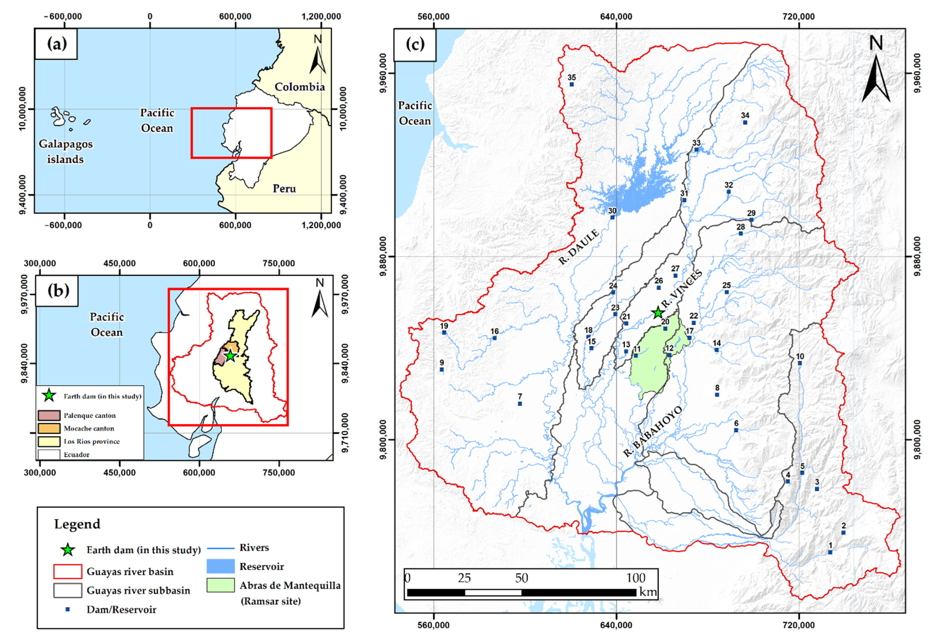
2. Study Area

3. Materials and Methods
3.1. Stage I: Dam Breach Analysis and Design
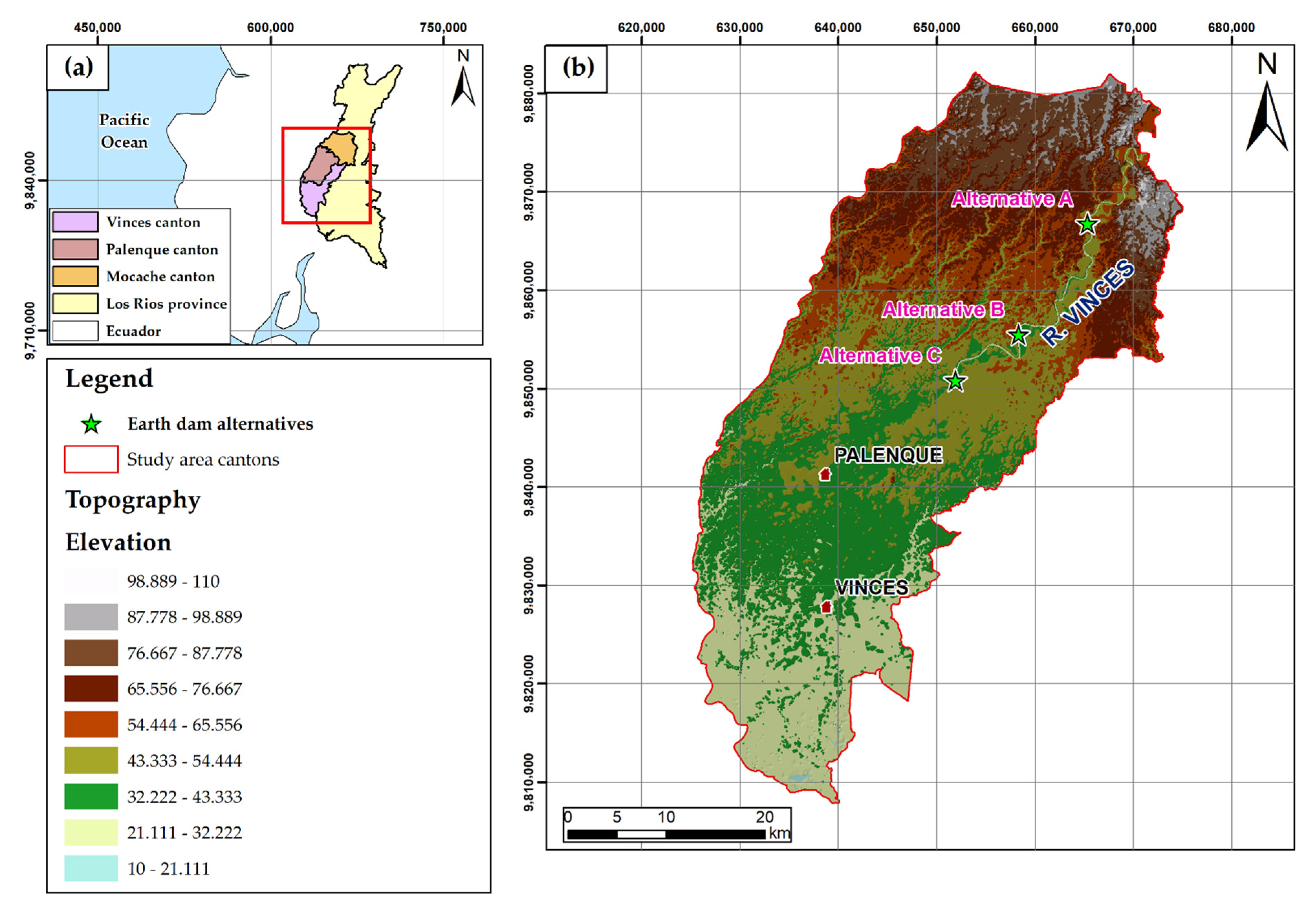
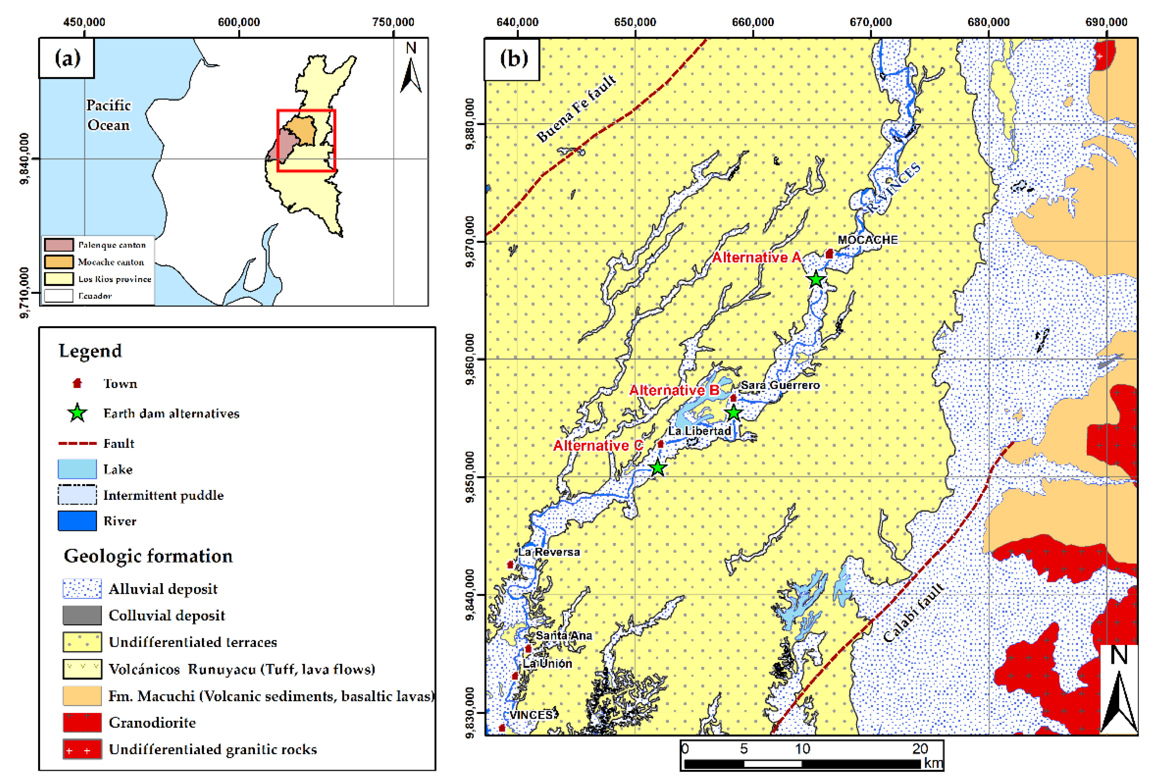
3.1.1. Topography and Soil Type
3.1.2. Seismic Risk
3.1.3. Social and Environmental Impact
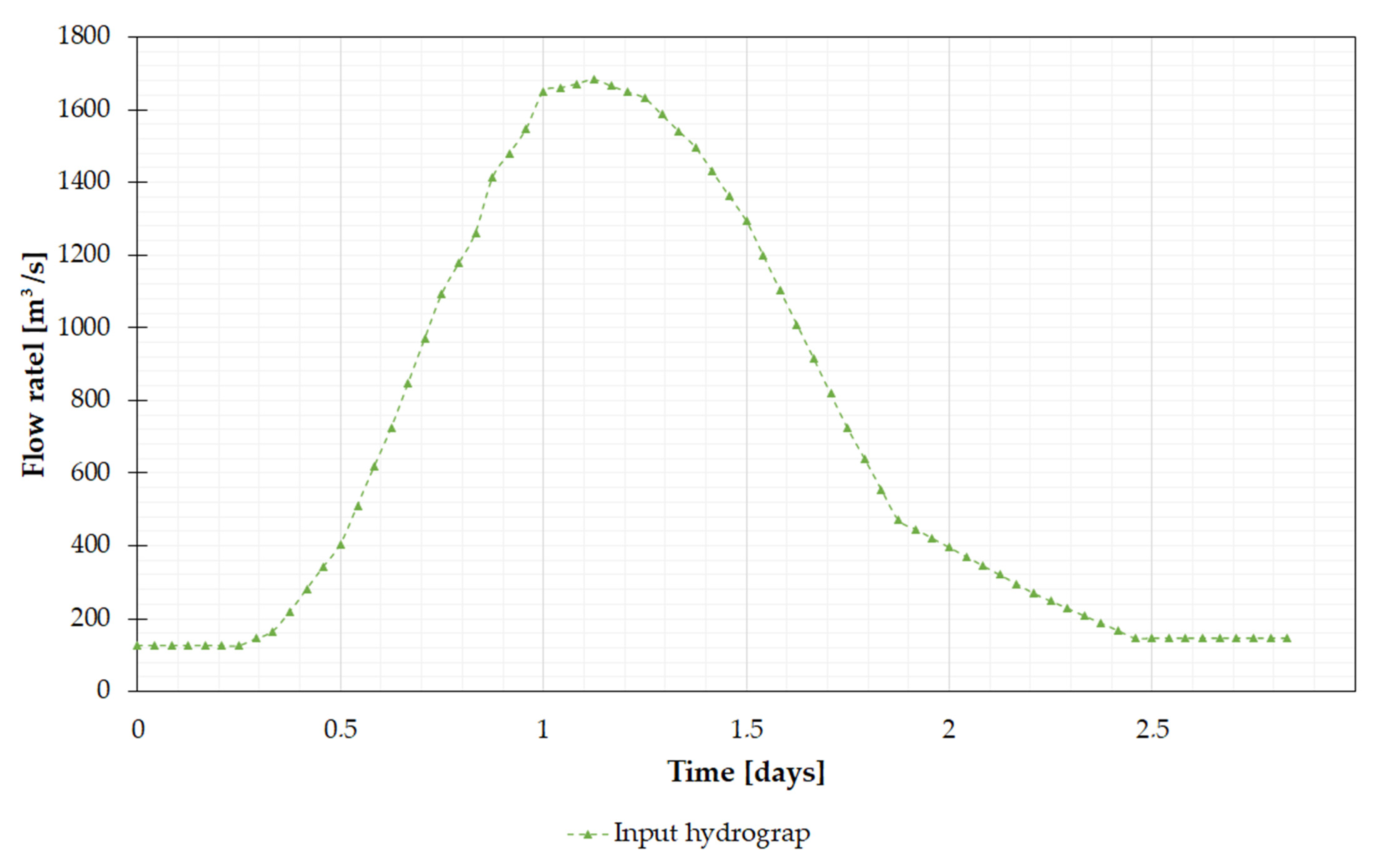
3.1.4. Hydrological Design
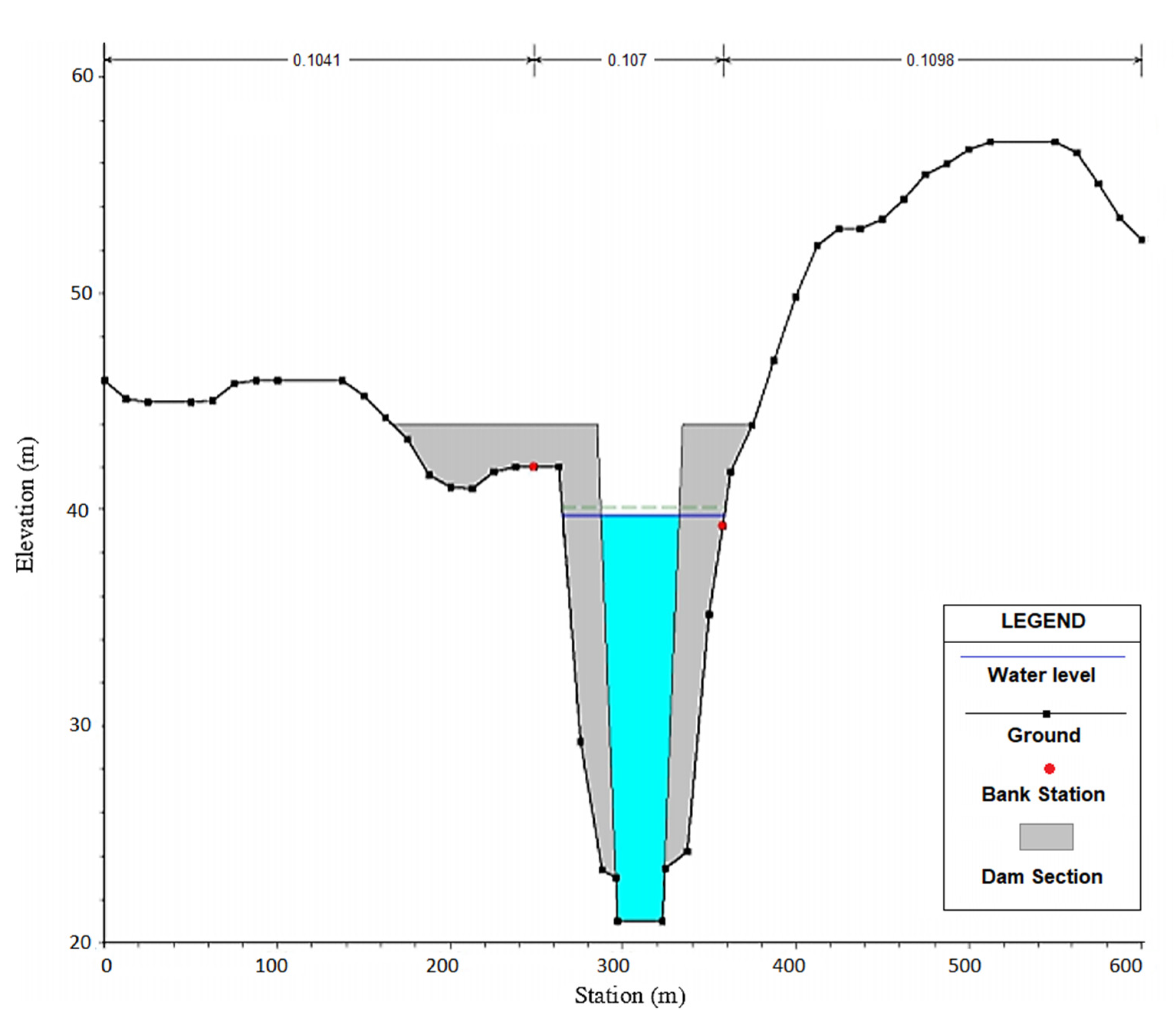
3.1.5. Hydraulic Design
- Effect of bottom irregularities and scour potential.
- Variations in the size and shape of channel cross-sections.
- : Presence of obstructions.
- : Vegetation and flow conditions.
- Correction factor for channel meanders.
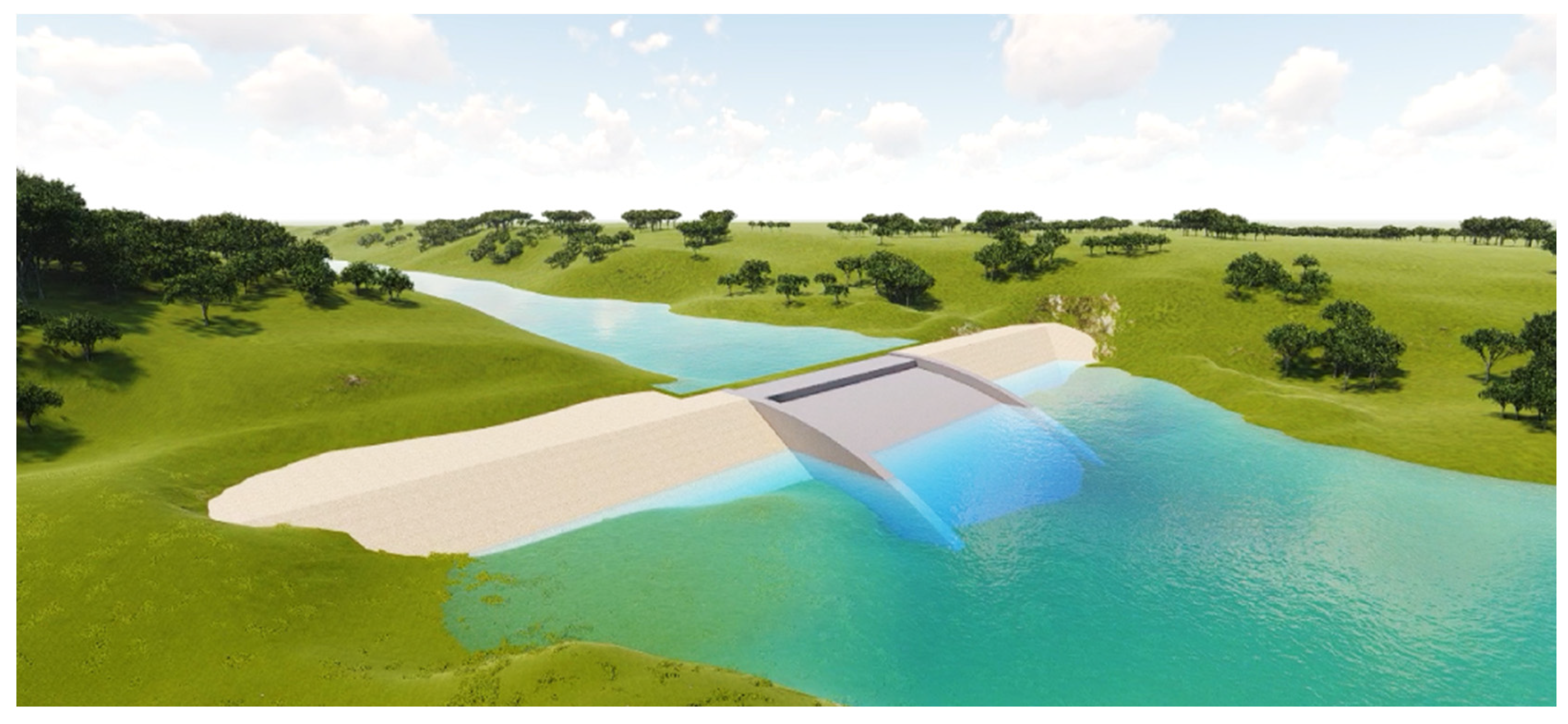
3.1.6. Location and Dam Type Selection
3.1.7. Dam Dimensioning
3.2. Stage II: Hydraulic Model Development
4. Results and Discussion
4.1. Dam Breach Analysis and Design
4.1.1. Topography and Soil Type
4.1.2. Seismic Risk
4.1.3. Social and Environmental Impact
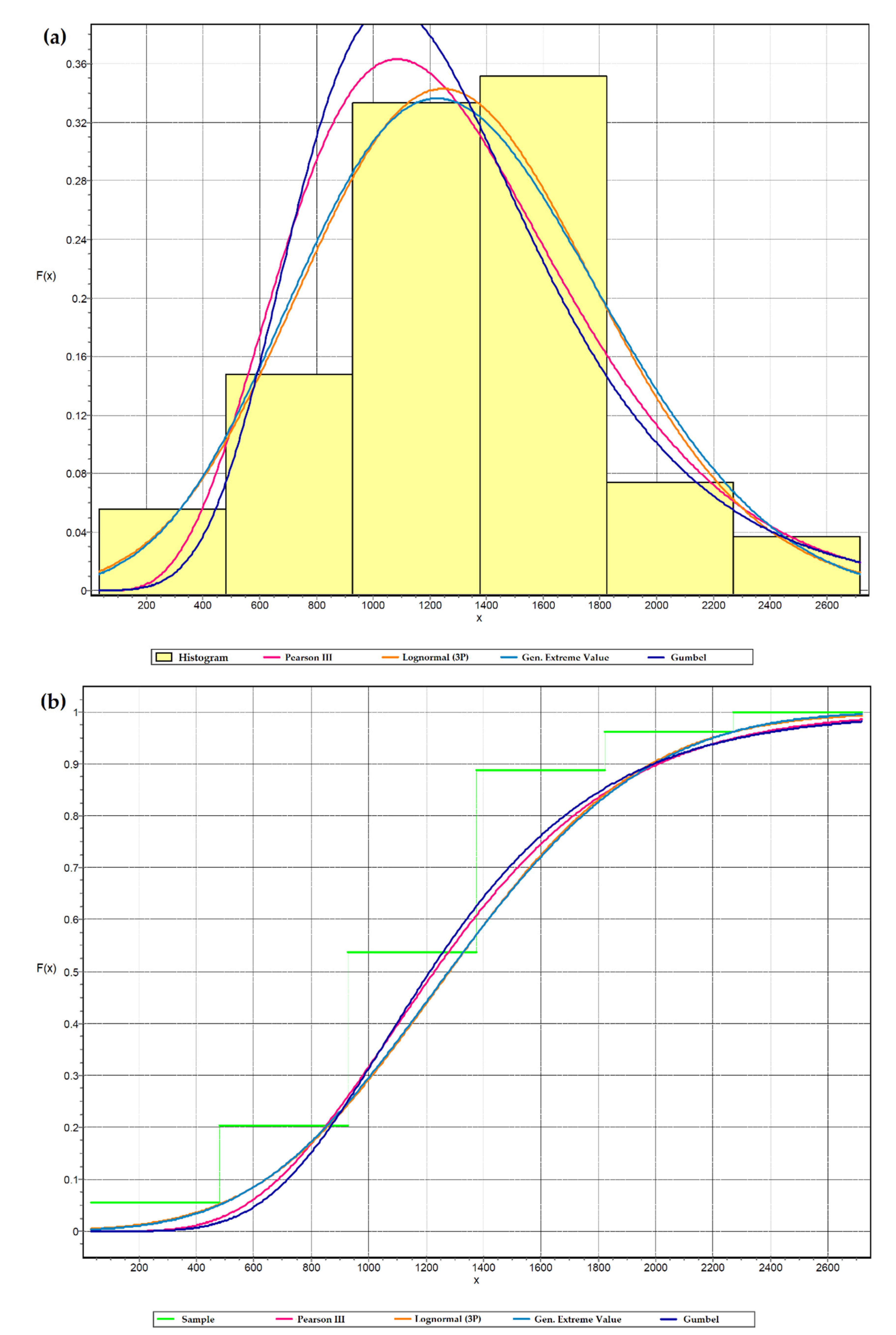
4.1.4. Hydrological Design
4.1.5. Hydraulic Design
4.1.6. Location and Dam Type Selection
4.1.7. Dam Dimensioning
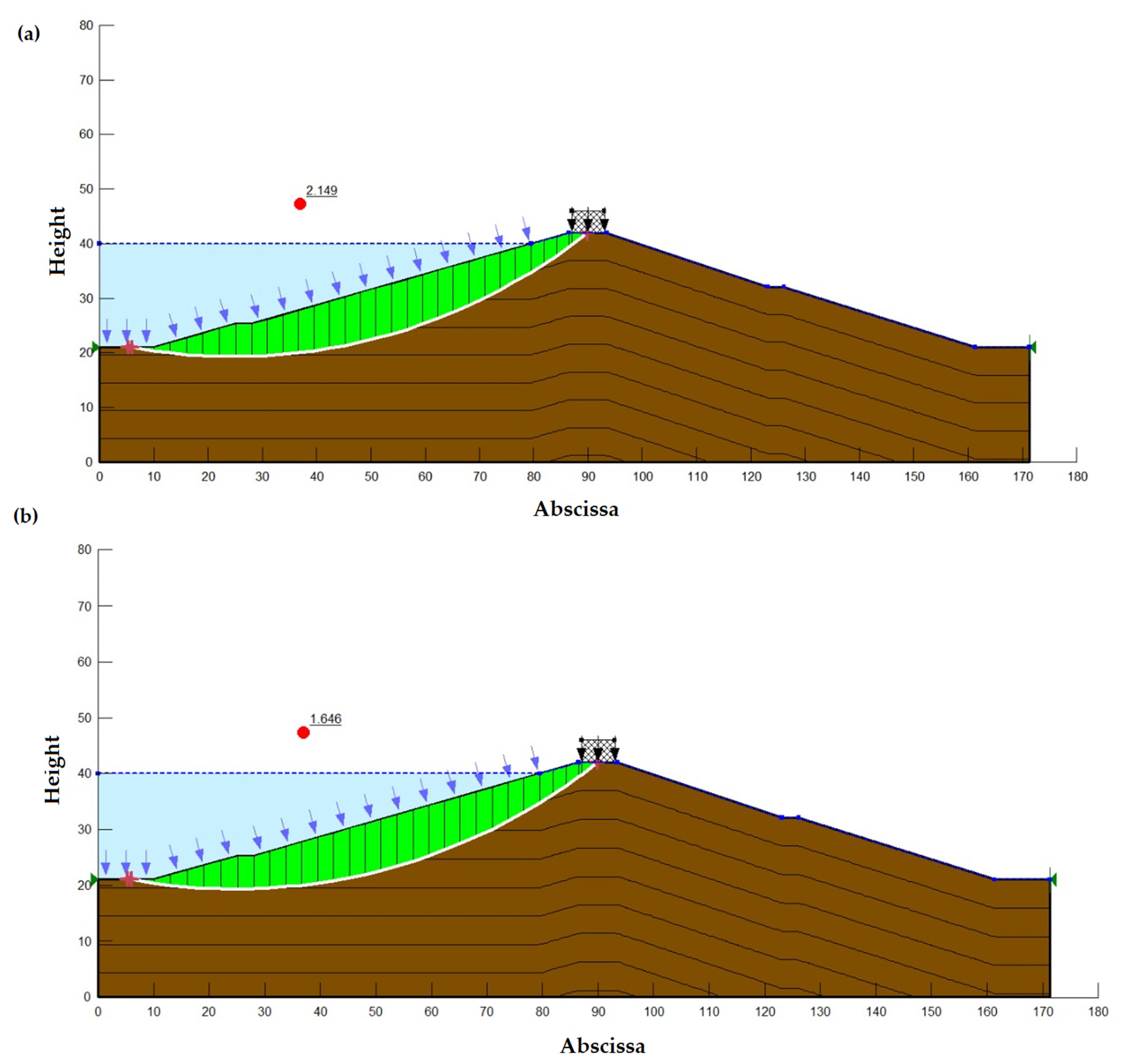
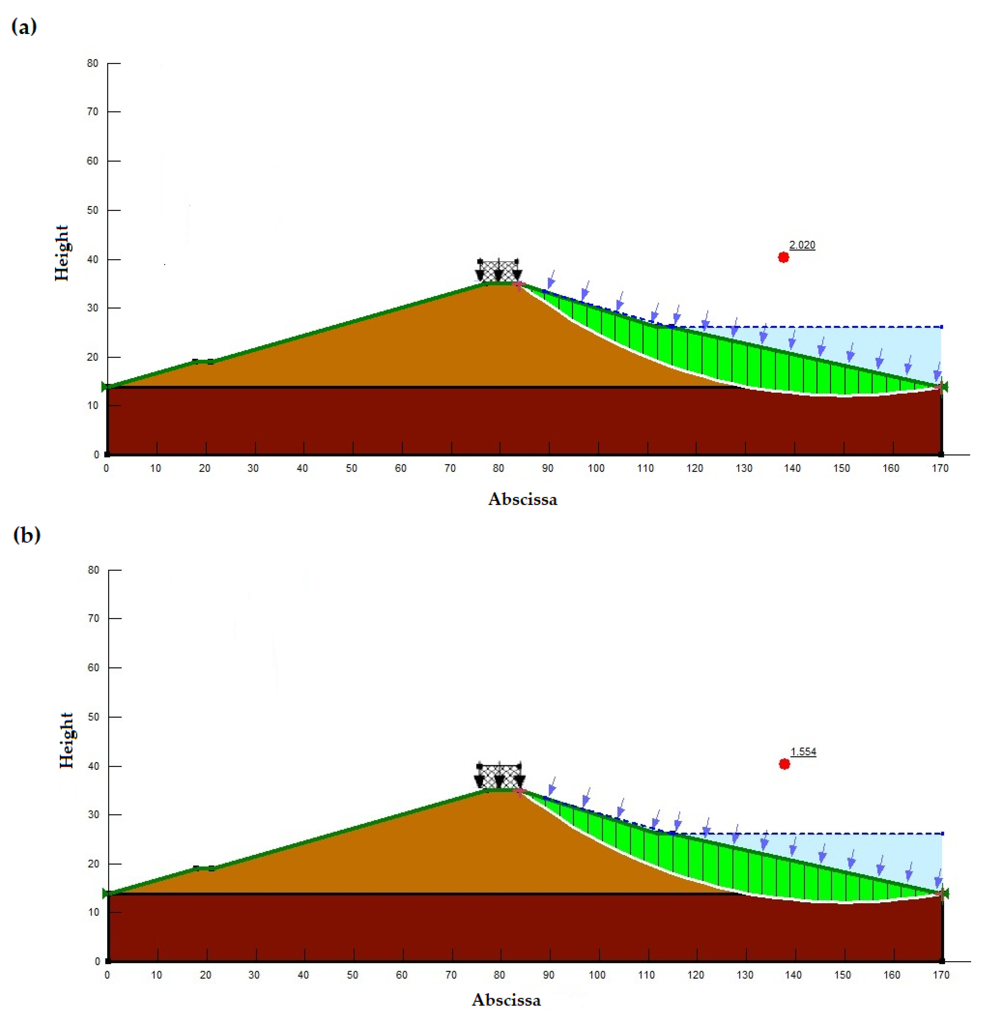
4.1.8. Verification
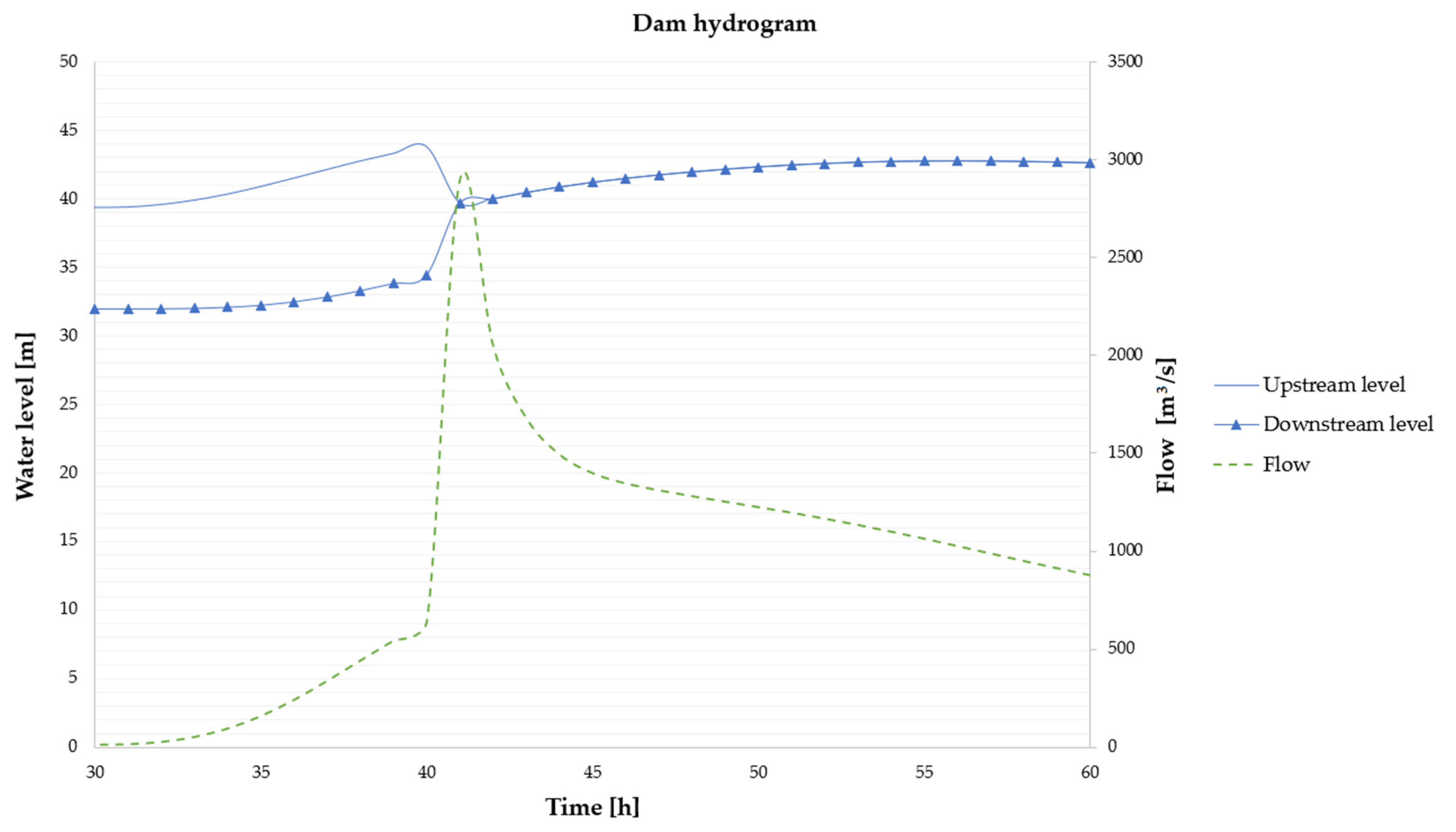
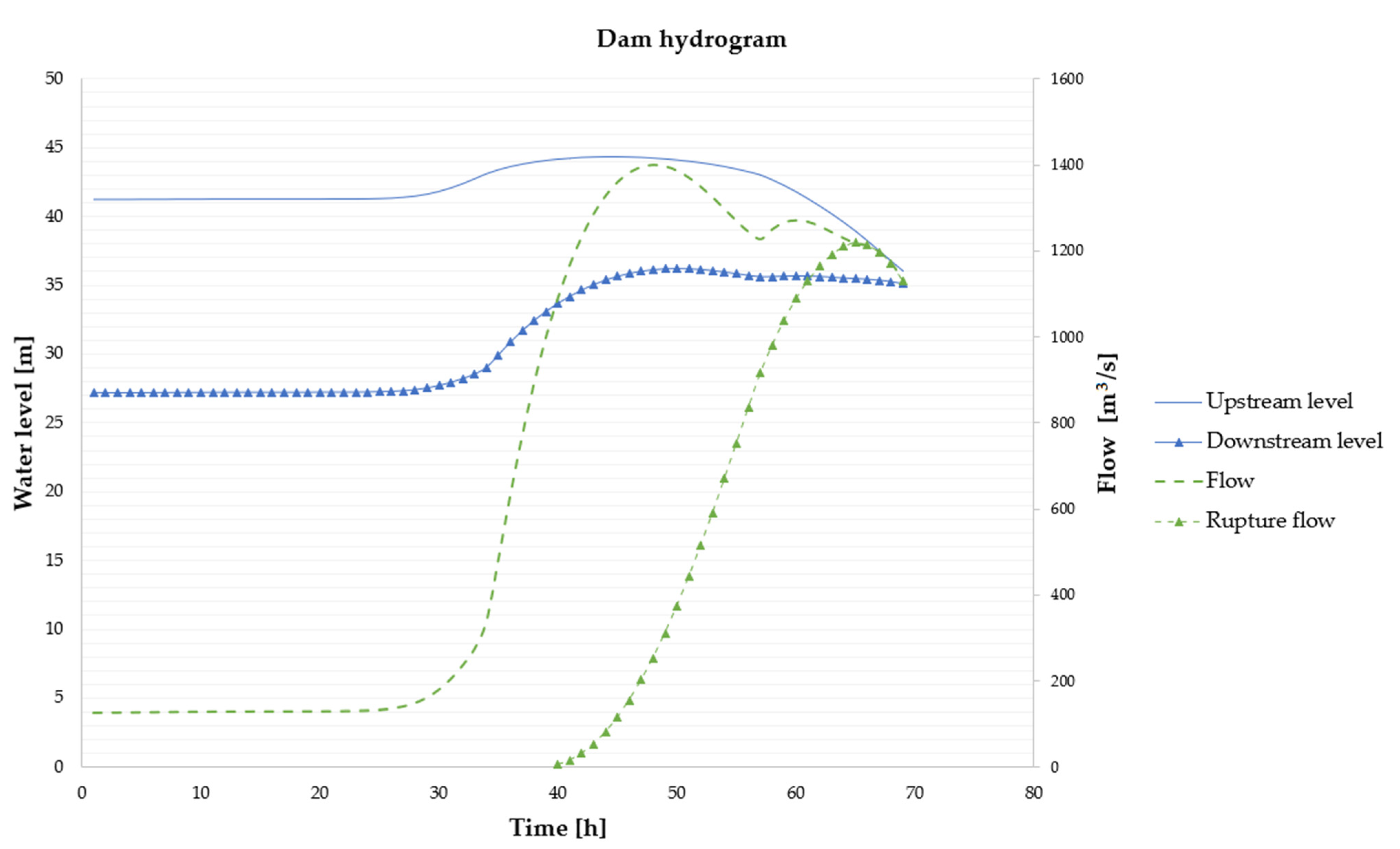
4.2. Hydraulic Model Development
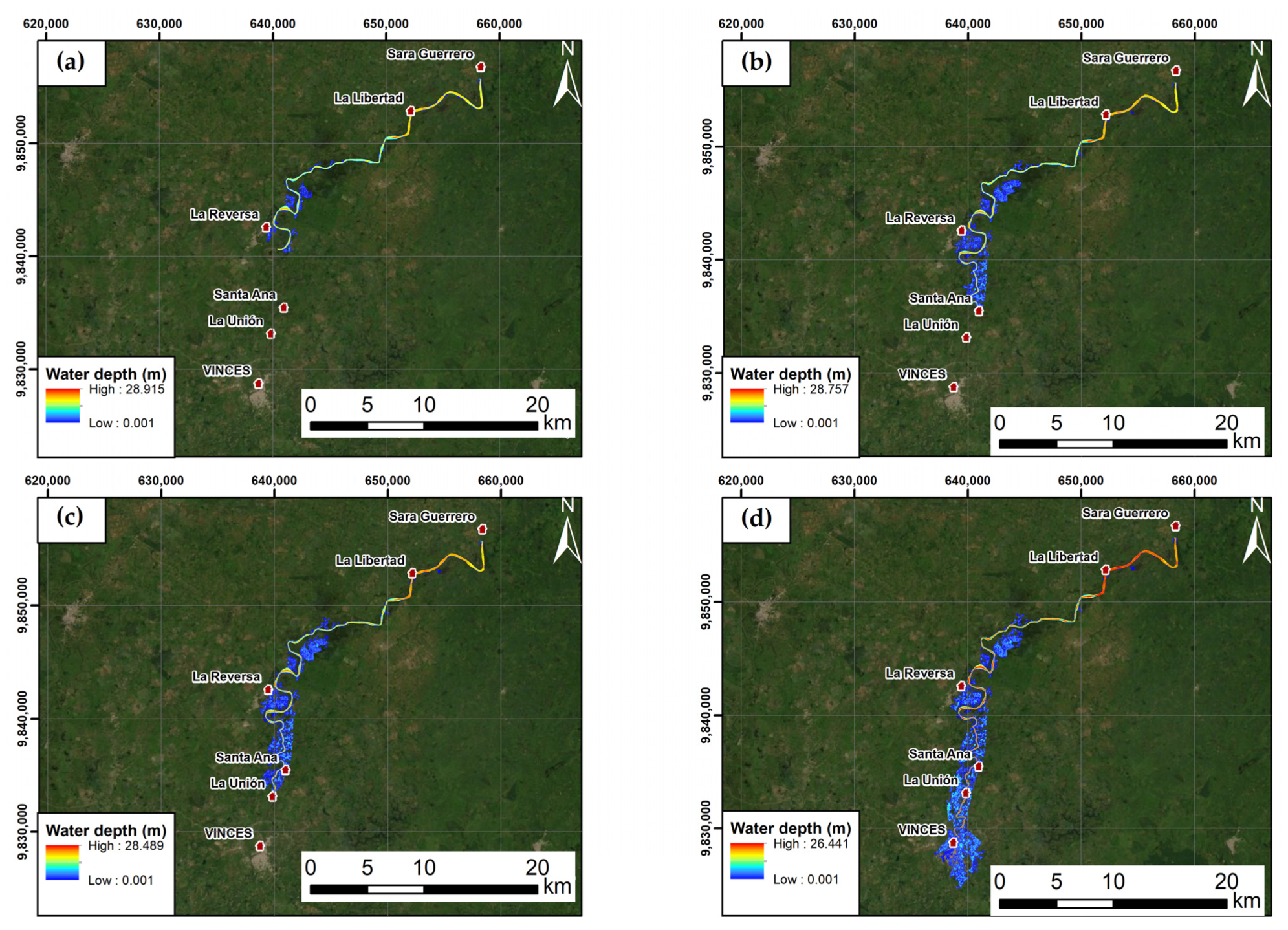
Flood Inundation Map
5. Conclusions
- (i)
- The dimensions of the designed dam were verified based on the safety and integrity of the structure through the stability of slopes and seismic conditions.
- (ii)
- The dam breach analysis encompasses a complex phenomenon where the transfer of the generated flow depends directly on parameters such as terrain roughness, edge conditions, time, and type of failure.
- (iii)
- The town closest to the dam downstream is “La Libertad”. However, this is not drastically affected by topographical conditions.
- (iv)
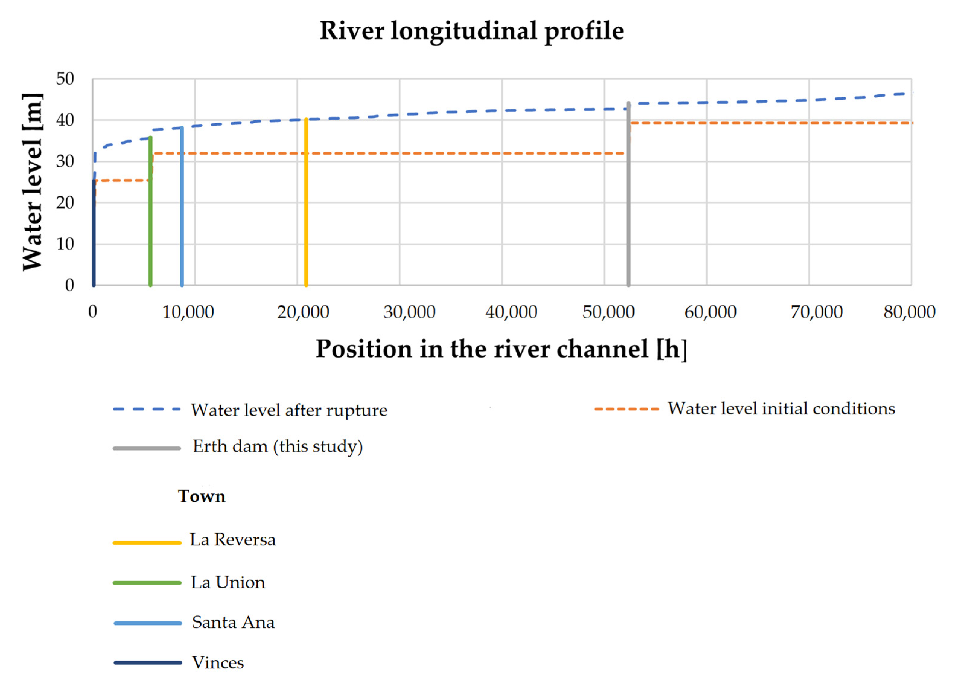
- At 31.35 km after the dam, the first flooded areas are identified, such as the “La Reversa” sector, where the water level rises to 8 m, mainly in considerably depressed sectors.
- (v)
- In real conditions of a dam failure, the behaviour of the resulting flow will be only an approximation to what is simulated in the software.
Supplementary Materials
Author Contributions
Funding
Institutional Review Board Statement
Informed Consent Statement
Data Availability Statement
Acknowledgments
Conflicts of Interest
References
- Wang, P.; Dong, S.; Lassoie, J.P. The Large Dam Dilemma: An Exploration of the Impacts of Hydro Projects on People and the Environment in China; Springer: Dordrecht, The Netherlands, 2014; ISBN 9789400776302. [Google Scholar]
- Schmutz, S.; Moog, O. Dams: Ecological Impacts and Management. In Riverine Ecosystem Management; Springer International Publishing: Cham, Switzerland, 2018; pp. 111–127. [Google Scholar]
- Altinbilek, D. The Role of Dams in Development. Water Sci. Technol. 2002, 45, 169–180. [Google Scholar] [CrossRef] [PubMed]
- Sayl, K.N.; Muhammad, N.S.; Yaseen, Z.M.; El-shafie, A. Estimation the Physical Variables of Rainwater Harvesting System Using Integrated GIS-Based Remote Sensing Approach. Water Resour. Manag. 2016, 30, 3299–3313. [Google Scholar] [CrossRef]
- Carrión-Mero, P.; Montalván, F.J.; Morante-Carballo, F.; Loor-Flores de Valgas, C.; Apolo-Masache, B.; Heredia, J. Flow and Transport Numerical Model of a Coastal Aquifer Based on the Hydraulic Importance of a Dyke and Its Impact on Water Quality. Manglaralto—Ecuador. Water 2021, 13, 443. [Google Scholar] [CrossRef]
- Carrión-Mero, P.; Morante-Carballo, F.; Briones-Bitar, J.; Herrera-Borja, P.; Chávez-Moncayo, M.; Arévalo-Ochoa, J. Design of a Technical-Artisanal Dike for Surface Water Storage and Artificial Recharge of the Manglaralto Coastal Aquifer. Santa Elena Parish, Ecuador. Int. J. Sustain. Dev. Plan. 2021, 16, 515–523. [Google Scholar] [CrossRef]
- Herrera-Franco, G.; Carrión-Mero, P.; Aguilar-Aguilar, M.; Morante-Carballo, F.; Jaya-Montalvo, M.; Morillo-Balsera, M.C. Groundwater Resilience Assessment in a Communal Coastal Aquifer System. The Case of Manglaralto in Santa Elena, Ecuador. Sustainability 2020, 12, 8290. [Google Scholar] [CrossRef]
- Carrión-Mero, P.; Morante-Carballo, F.; Vargas-Ormaza, V.; Apolo-Masache, B.; Jaya-Montalvo, M. A Conceptual Socio-Hydrogeological Model Applied to Sustainable Water Management. Case Study of the Valdivia River Basin, Southwestern Ecuador. Int. J. Sustain. Dev. Plan. 2021, 16, 1275–1285. [Google Scholar] [CrossRef]
- Singh, V.P. Dam Breach Modeling Technology; Water Science and Technology Library; Springer: Dordrecht, The Netherlands, 1996; Volume 17, ISBN 978-90-481-4668-0. [Google Scholar]
- Charles, J.A.; Tančev, L.; Herschy, R.W.; Herschy, R.W.; Cederwall, K.; Gertman, I.; Herschy, R.W.; Herschy, R.W.; Terzhevik, A.; Golosov, S.; et al. Dam Failures: Impact on Reservoir Safety Legislation in Great Britain; Bengtsson, L., Herschy, R.W., Fairbridge, R.W., Eds.; Encyclopedia of Earth Sciences Series; Springer: Dordrecht, The Netherlands, 2012; pp. 177–186. ISBN 9781402044106. [Google Scholar]
- Goldin, A.L.; Rasskazov, L.N. Design of Earth Dams; Zeidler, R.B., Ed.; Routledge: London, UK, 1987; ISBN 9781315141022. [Google Scholar]
- Kutzner, C. Earth and Rockfill Dams: Principles for Design and Construction; Routledge: London, UK, 2017; ISBN 9780203758991. [Google Scholar]
- Titova, T.S.; Longobardi, A.; Akhtyamov, R.G.; Nasyrova, E.S. Lifetime of Earth Dams. Mag. Civ. Eng. 2017, 69, 34–43. [Google Scholar] [CrossRef]
- Pisaniello, J.D.; McKay, J.M. A Farmer-Friendly Dam Safety Evaluation Procedure as a Key Part of Modern Australian Water Laws. Water Int. 2003, 28, 90–102. [Google Scholar] [CrossRef]
- Stephens, T. Manual on Small Earth Dams: A Guide to Siting, Design and Construction; Food and Agriculture Organization of the United Nations (FAO): Rome, Italy, 2010; ISBN 9789251065471. [Google Scholar]
- Sun, Y.; Chang, H.; Miao, Z.; Zhong, D. Solution Method of Overtopping Risk Model for Earth Dams. Saf. Sci. 2012, 50, 1906–1912. [Google Scholar] [CrossRef]
- Cloete, G.C.; Retief, J.V.; Viljoen, C. A Rational Quantitative Optimal Approach to Dam Safety Risk Reduction. Civ. Eng. Environ. Syst. 2016, 33, 85–105. [Google Scholar] [CrossRef]
- Shahraki, A.; Zadbar, A.; Motevalli, M.; Aghajani, F. Modeling of Earth Dam Break with SMPDBK Case Study: Bidekan Earth Dam. World Appl. Sci. 2012, 376–386. [Google Scholar] [CrossRef]
- Urzică, A.; Mihu-Pintilie, A.; Stoleriu, C.C.; Cîmpianu, C.I.; Huţanu, E.; Pricop, C.I.; Grozavu, A. Using 2D HEC-RAS Modeling and Embankment Dam Break Scenario for Assessing the Flood Control Capacity of a Multi-Reservoir System (NE Romania). Water 2020, 13, 57. [Google Scholar] [CrossRef]
- Albu, L.-M.; Enea, A.; Iosub, M.; Breabăn, I.-G. Dam Breach Size Comparison for Flood Simulations. A HEC-RAS Based, GIS Approach for Drăcșani Lake, Sitna River, Romania. Water 2020, 12, 1090. [Google Scholar] [CrossRef]
- Brunner, G. HEC-RAS River Analysis System Hydraulic Reference Manual, Version 5.0; USACE: Washington, DC, USA, 2016; Volume 547. [Google Scholar]
- Brunner, G. HEC-RAS River Analysis System. Hydraulic User’s Manual, Version 6.0; USACE: Washington, DC, USA, 2021; pp. 456–594. [Google Scholar]
- Psomiadis, E.; Tomanis, L.; Kavvadias, A.; Soulis, K.X.; Charizopoulos, N.; Michas, S. Potential Dam Breach Analysis and Flood Wave Risk Assessment Using HEC-RAS and Remote Sensing Data: A Multicriteria Approach. Water 2021, 13, 364. [Google Scholar] [CrossRef]
- Costabile, P.; Costanzo, C.; Ferraro, D.; Macchione, F.; Petaccia, G. Performances of the New HEC-RAS Version 5 for 2-D Hydrodynamic-Based Rainfall-Runoff Simulations at Basin Scale: Comparison with a State-of-the Art Model. Water 2020, 12, 2326. [Google Scholar] [CrossRef]
- Zeiger, S.J.; Hubbart, J.A. Measuring and Modeling Event-Based Environmental Flows: An Assessment of HEC-RAS 2D Rain-on-Grid Simulations. J. Environ. Manag. 2021, 285, 112125. [Google Scholar] [CrossRef]
- Mokhtari, F.; Soltani, S.; Mousavi, S.A. Assessment of Flood Damage on Humans, Infrastructure, and Agriculture in the Ghamsar Watershed Using HEC-FIA Software. Nat. Hazards Rev. 2017, 18, 04017006. [Google Scholar] [CrossRef]
- Memoria Técnica. Cantón Mocache. Proyecto: Generación de Geoinformación Para La Gestión Del Territorio a Nivel Nacional Escala 1:25,000. Componente 5: “Socioeconómico y Cultural”. 2012. Available online: http://app.sni.gob.ec/sni-link/sni/PDOT/ZONA5/NIVEL_DEL_PDOT_CANTONAL/LOS_RIOS/MOCACHE/IEE/MEMORIAS_TECNICAS/mt_mocache_socioeconomico.pdf (accessed on 10 June 2022).
- SIPA. Sistema de Información Pública Agropecuaria. Available online: http://sipa.agricultura.gob.ec/index.php/sipa-estadisticas/estadisticas-productivas (accessed on 15 July 2021).
- INEC. Población y Demografía. Available online: https://www.ecuadorencifras.gob.ec/censo-de-poblacion-y-vivienda/ (accessed on 13 July 2021).
- Arias-Hidalgo, M.; Villa-Cox, G.; Griensven, A.V.; Solórzano, G.; Villa-Cox, R.; Mynett, A.E.; Debels, P. A Decision Framework for Wetland Management in a River Basin Context: The “Abras de Mantequilla” Case Study in the Guayas River Basin, Ecuador. Environ. Sci. Policy 2013, 34, 103–114. [Google Scholar] [CrossRef]
- Ramsar Ramsar Sites Information Service. Available online: https://rsis.ramsar.org/ris/1023 (accessed on 13 July 2021).
- SENAGUA. Embalse. Escala 1:250,000. Available online: http://ide.ambiente.gob.ec/mapainteractivo/ (accessed on 13 July 2021).
- MAGAP. Cartas Geológicas. Escala 1:100,000. Available online: https://sni.gob.ec/coberturas (accessed on 7 June 2021).
- SNGRE. Geoportal-SNGRE. Available online: https://srvportal.gestionderiesgos.gob.ec/portal/home/ (accessed on 6 September 2021).
- INAMHI. Red de Estaciones Meteorológicas e Hidrológicas. Available online: https://inamhi.wixsite.com/inamhi/novedades (accessed on 21 September 2021).
- MIDUVI. Ministerio de Desarrollo Urbano y Vivienda—MIDUVI. Available online: https://www.habitatyvivienda.gob.ec/documentos-normativos-nec-norma-ecuatoriana-de-la-construccion/ (accessed on 6 September 2021).
- Zhu, G.; Sang, L.; Zhang, Z.; Sun, Z.; Ma, H.; Liu, Y.; Zhao, K.; Wang, L.; Guo, H. Impact of Landscape Dams on River Water Cycle in Urban and Peri-Urban Areas in the Shiyang River Basin: Evidence Obtained from Hydrogen and Oxygen Isotopes. J. Hydrol. 2021, 602, 126779. [Google Scholar] [CrossRef]
- Conesa Fernández-Vítora, V.; Conesa Ripoll, L.; Conesa Ripoll, V.; Bolea, E.; Teresa, M.; Ros Garo, V. Guía Metodológica Para la Evaluación del Impacto Ambiental; Mundi-Prensa: Madrid, España, 1993. [Google Scholar]
- INAMHI. Biblioteca-Instituto Nacional de Meteorología e Hidrología. Available online: https://www.inamhi.gob.ec/biblioteca/ (accessed on 9 September 2021).
- Gumbel, E.J. Statistics of Extremes; Columbia University Press: New York, NY, USA, 1958; ISBN 9780231891318. [Google Scholar]
- Galton, F. The Geometric Mean, in Vital and Social Statistics. Proc. R. Soc. London 1879, 29, 365–367. [Google Scholar] [CrossRef]
- Pearson, K. Contributions to the Mathematical Theory of Evolution. Skew Variation in Homogeneous Material. Philos. Trans. R. Soc. Lond. 1895, 186, 343–414. [Google Scholar] [CrossRef] [Green Version]
- Pearson, K. Mathematical Contributions to the Theory of Evolution. Supplement to a Memoir on Skew Variation. Philos. Trans. R. Soc. Lond. Ser. A Contain. Pap. Math. Phys. Character 1901, 197, 443–459. [Google Scholar] [CrossRef] [Green Version]
- Pearson, K. On the Probable Error of a Coefficient of Mean Square Contingency. Biometrika 1915, 10, 570. [Google Scholar] [CrossRef]
- Lilliefors, H.W. On the Kolmogorov-Smirnov Test for Normality with Mean and Variance Unknown. J. Am. Stat. Assoc. 1967, 62, 399–402. [Google Scholar] [CrossRef]
- Chugaev, R.R. Hydraulic Structures. Part II. Overflow Diversion Dams; Agropromizdat: Moscow, Russia, 1985. (In Russian) [Google Scholar]
- Bakhmeteff, B.A. Hydraulics of Open Channels; McGraw-Hill: New York, NY, USA, 1932. [Google Scholar]
- Cowan, W.L. Estimating Hydraulic Roughness Coefficients. Agric. Eng. 1956, 37, 473–475. [Google Scholar]
- Burt, R. Soil Survey Field and Laboratory Methods Manual; Soil Survey Staff, Ed.; U.S. Department of Agriculture: Washington, DC, USA, 2014.
- Arcement, G.J.; Schneider, V.R. Guide for Selecting Manning’s Roughness Coefficients for Natural Channels and Flood Plains United States Geological Survey Water-Supply Paper 2339; U.S. Geological Survey: Liston, VG, USA, 1989.
- Likert, R. A Technique for the Measurement of Attitudes. Arch. Psychol. 1932, 140, 1–22. [Google Scholar]
- Pagano, L.; Sica, S. Earthquake Early Warning for Earth Dams: Concepts and Objectives. Nat. Hazards 2013, 66, 303–318. [Google Scholar] [CrossRef]
- Sandoval, W. Diseño de Obras Hidrotécnicas; EDIESPE; Comisión Editorial de la Universidad de las Fuerzas Armadas ESPE: Sangolquí, Ecuador, 2018; ISBN 978-9942-35-390-0. [Google Scholar]
- Buldeya, V. Construcciones Para el Manejo del Agua en Pequeños Ríos (En Ruso); Budivelnik: Kiev, Ukraine, 1977. [Google Scholar]
- USACE. Gravity Dam Design. In USACE Engineer Manual; USACE: Washington, DC, USA, 1995; pp. 1–88. ISBN EM-1110-2-2200. [Google Scholar]
- US Bureau of Reclamation. Design Standards No. 14 Spillways and Outlet Works Design Standard; US Bureau of Reclamation: Washington, DC, USA, 2014.
- Gogoaşe Nistoran, D.E.; Gheorghe Popovici, D.A.; Savin, B.A.C.; Armaş, I. GIS for Dam-Break Flooding. Study Area: Bicaz-Izvorul Muntelui (Romania). In Space and Time Visualisation; Boştenaru Dan, M., Crăciun, C., Eds.; Springer International Publishing: Cham, Switzerland, 2016; pp. 253–280. [Google Scholar]
- Froehlich, D.C. Peak Outflow from Breached Embankment Dam. J. Water Resour. Plan. Manag. 1995, 121, 90–97. [Google Scholar] [CrossRef]
- Froehlich, D.C. Embankment Dam Breach Parameters and Their Uncertainties. J. Hydraul. Eng. 2008, 134, 1708–1721. [Google Scholar] [CrossRef]
- Costabile, P.; Costanzo, C.; Ferraro, D.; Barca, P. Is HEC-RAS 2D Accurate Enough for Storm-Event Hazard Assessment? Lessons Learnt from a Benchmarking Study Based on Rain-on-Grid Modelling. J. Hydrol. 2021, 603, 126962. [Google Scholar] [CrossRef]
- Pasquier, U.; He, Y.; Hooton, S.; Goulden, M.; Hiscock, K.M. An Integrated 1D–2D Hydraulic Modelling Approach to Assess the Sensitivity of a Coastal Region to Compound Flooding Hazard under Climate Change. Nat. Hazards 2019, 98, 915–937. [Google Scholar] [CrossRef] [Green Version]
- MAGAP. Hidrogeológico. Escala 1:100,000. Available online: http://qa-ide.ambiente.gob.ec:8080/geonetwork/srv/api/records/1535d6a9-57ec-49af-94d3-f2e8e2dc2a43 (accessed on 7 June 2021).
- Egüez, A.; Alvarado, A.; Yepes, H. Map of Quaternary Faults and Folds of Ecuador and Its Offshore Regions. US Geol. Surv. Open-File Rep. 2003, 3, 289. [Google Scholar]
- de Sherbinin, A.; Castro, M.; Gemenne, F.; Cernea, M.M.; Adamo, S.; Fearnside, P.M.; Krieger, G.; Lahmani, S.; Oliver-Smith, A.; Pankhurst, A.; et al. Preparing for Resettlement Associated with Climate Change. Science 2011, 334, 456–457. [Google Scholar] [CrossRef] [PubMed]
- Shi, G.; Zhou, J.; Yu, Q. Resettlement in China. In Impacts of Large Dams: A Global Assessment; Tortajada, C., Altinbilek, D., Biswas, A., Eds.; Springer: Berlin/Heidelberg, Germany, 2012; pp. 219–241. [Google Scholar]
- Revelo, W. Aspectos Biológicos y Pesqueros de Los Principales Peces Del Sistema Hídrico de La Provincia de Los Ríos, Durante 2009. Bol. Cient. Téc. 2010, 20, 53–84. [Google Scholar]
- Acharya, B.; Joshi, B. Flood Frequency Analysis for an Ungauged Himalayan River Basin Using Different Methods: A Case Study of Modi Khola, Parbat, Nepal. Meteorol. Hydrol. Water Manag. 2020, 8, 46–51. [Google Scholar] [CrossRef]
- Gil, M.Á.; González-Rodríguez, G. Fuzzy vs. Likert Scale in Statistics. In Combining Experimentation and Theory. Studies in Fuzziness and Soft Computing; Trillas, E., Bonissone, P., Magdalena, L., Kacprzyk, J., Eds.; Springer: Berlin/Heidelberg, Germany, 2012; pp. 407–420. [Google Scholar]
- Souter, N.; Shaad, K.; Vollmer, D.; Regan, H.; Farrell, T.; Arnaiz, M.; Meynell, P.-J.; Cochrane, T.; Arias, M.; Piman, T.; et al. Using the Freshwater Health Index to Assess Hydropower Development Scenarios in the Sesan, Srepok and Sekong River Basin. Water 2020, 12, 788. [Google Scholar] [CrossRef] [Green Version]
- Kirshen, P.; Aytur, S.; Hecht, J.; Walker, A.; Burdick, D.; Jones, S.; Fennessey, N.; Bourdeau, R.; Mather, L. Integrated Urban Water Management Applied to Adaptation to Climate Change. Urban Clim. 2018, 24, 247–263. [Google Scholar] [CrossRef]
- Kittipongvises, S.; Phetrak, A.; Rattanapun, P.; Brundiers, K.; Buizer, J.L.; Melnick, R. AHP-GIS Analysis for Flood Hazard Assessment of the Communities Nearby the World Heritage Site on Ayutthaya Island, Thailand. Int. J. Disaster Risk Reduct. 2020, 48, 101612. [Google Scholar] [CrossRef]
- Yildiz, A.E.; Dikmen, I.; Birgonul, M.T.; Ercoskun, K.; Alten, S. A Knowledge-Based Risk Mapping Tool for Cost Estimation of International Construction Projects. Autom. Constr. 2014, 43, 144–155. [Google Scholar] [CrossRef]
- Jamali, A.A.; Ghorbani Kalkhajeh, R. Spatial Modeling Considering Valley’s Shape and Rural Satisfaction in Check Dams Site Selection and Water Harvesting in the Watershed. Water Resour. Manag. 2020, 34, 3331–3344. [Google Scholar] [CrossRef]
- Park, C.; Han, S.; Lee, K.-W.; Lee, Y. Analyzing Drivers of Conflict in Energy Infrastructure Projects: Empirical Case Study of Natural Gas Pipeline Sectors. Sustainability 2017, 9, 2031. [Google Scholar] [CrossRef] [Green Version]
- MacDonald, T.C.; Langridge-Monopolis, J. Breaching Charateristics of Dam Failures. J. Hydraul. Eng. 1984, 110, 567–586. [Google Scholar] [CrossRef]
- Evans, S.G. The Maximum Discharge of Outburst Floods Caused by the Breaching of Man-Made and Natural Dams. Can. Geotech. J. 1986, 23, 385–387. [Google Scholar] [CrossRef]
- Kirkpatrick, J.I.M.; Olbert, A.I. Modelling the Effects of Climate Change on Urban Coastal-Fluvial Flooding. J. Water Clim. Chang. 2020, 11, 270–288. [Google Scholar] [CrossRef] [Green Version]
- Bharath, A.; Shivapur, A.V.; Hiremath, C.G.; Maddamsetty, R. Dam Break Analysis Using HEC-RAS and HEC-GeoRAS: A Case Study of Hidkal Dam, Karnataka State, India. Environ. Chall. 2021, 5, 100401. [Google Scholar] [CrossRef]
- Desta, H.B.; Belayneh, M.Z. Dam Breach Analysis: A Case of Gidabo Dam, Southern Ethiopia. Int. J. Environ. Sci. Technol. 2021, 18, 107–122. [Google Scholar] [CrossRef]
- Hailu, M.B. Modeling Assessment of Seepage and Slope Stability of Dam under Static and Dynamic Conditions of Grindeho Dam in Ethiopia. Model. Earth Syst. Environ. 2021, 7, 2231–2239. [Google Scholar] [CrossRef]
- Salmasi, F.; Pradhan, B.; Nourani, B. Prediction of the Sliding Type and Critical Factor of Safety in Homogeneous Finite Slopes. Appl. Water Sci. 2019, 9, 158. [Google Scholar] [CrossRef] [Green Version]
- Shole, D.G.; Belayneh, M.Z. The Effect of Side Slope and Clay Core Shape on the Stability of Embankment Dam: Southern Ethiopia. Int. J. Environ. Sci. Technol. 2019, 16, 5871–5880. [Google Scholar] [CrossRef]
- Hess, D.M.; Leshchinsky, B.A.; Bunn, M.; Benjamin Mason, H.; Olsen, M.J. A Simplified Three-Dimensional Shallow Landslide Susceptibility Framework Considering Topography and Seismicity. Landslides 2017, 14, 1677–1697. [Google Scholar] [CrossRef]
- Wang, R.-H.; Li, D.-Q.; Wang, M.-Y.; Liu, Y. Deterministic and Probabilistic Investigations of Piping Occurrence during Tunneling through Spatially Variable Soils. ASCE-ASME J. Risk Uncertain. Eng. Syst. Part A Civ. Eng. 2021, 7, 04021009. [Google Scholar] [CrossRef]
- Wang, R.-H.; Sun, P.-G.; Li, D.-Q.; Tyagi, A.; Liu, Y. Three-Dimensional Seepage Investigation of Riverside Tunnel Construction Considering Heterogeneous Permeability. ASCE-ASME J. Risk Uncertain. Eng. Syst. Part A Civ. Eng. 2021, 7, 04021041. [Google Scholar] [CrossRef]
- Nedrigi, V.P. Designer’s Handbook. Hydraulic Structures; Stroiizdat: Moscow, Russia, 1983. (In Russian) [Google Scholar]
- Ministerio de Obras Públicas de España. Instrucción Para Proyecto, Construcción y Explotación de Grandes Presas; Ministerio de Obras Públicas de España: Madrid, Spain, 1967.


| Alternatives | Towns | Population | Total |
|---|---|---|---|
| A | Las Campanas | 480 | 1827 |
| La Porfia | 320 | ||
| Emperatriz | 387 | ||
| Buena Aventura | 340 | ||
| Gramalotillo | 300 | ||
| B | Sara Guerrero | 487 | 487 |
| C | La Libertad | 526 | 526 |
| Total | 2840 | ||
| Flows along the Vinces River [m3/s] | ||||
|---|---|---|---|---|
| Station: Quevedo | ||||
| Return period [years] | Gumbel | GEV I | Log Normal | Pearson III |
| 100 | 549.7 | 481.3 | 705.5 | 511.6 |
| 200 | 600.3 | 527.3 | 811.1 | 568.2 |
| 500 | 667.0 | 588.0 | 960.4 | 643.9 |
| Station: Vinces | ||||
| Return period [years] | Gumbel | GEV I | Log Normal | Pearson III |
| 100 | 1326.0 | 1225.1 | 1187.1 | 1252.3 |
| 200 | 1396.7 | 1288.5 | 1230.4 | 1323.7 |
| 500 | 1489.9 | 1372.0 | 1284.8 | 1418.4 |
| Gumbel | GEV I | Log Normal | Pearson III | |
|---|---|---|---|---|
| 1 | 4.5% | 5.0% | 13.1% | 0.6% |
| 2 | 12% | |||
| Fit | Accept | Accept | Reject | Accept |
| Alternative | Yc [m] | Yn [m] |
|---|---|---|
| A | 2.004 | 16.253 |
| B | 4.201 | 16.304 |
| C | 2.581 | 15.674 |
| Quantifying Parameters | Score | |||||
|---|---|---|---|---|---|---|
| 5 | 4 | 3 | 2 | 1 | ||
| Alternative A | Seismic risk | x | ||||
| Environmental impact | x | |||||
| Social impact | x | |||||
| Geological faults | x | |||||
| Soil type | x | |||||
| Topography | x | |||||
| Hydraulics | x | |||||
| Economy | x | |||||
| Total | 20 | |||||
| Alternative B | Seismic risk | x | ||||
| Environmental impact | x | |||||
| Social impact | x | |||||
| Geological faults | x | |||||
| Soil type | x | |||||
| Topography | x | |||||
| Hydraulics | x | |||||
| Economy | x | |||||
| Total | 25 | |||||
| Alternative C | Seismic risk | x | ||||
| Environmental impact | x | |||||
| Social impact | x | |||||
| Geological faults | x | |||||
| Soil type | x | |||||
| Topography | x | |||||
| Hydraulics | x | |||||
| Economy | x | |||||
| Total | 24 | |||||
| Alternative B | |
|---|---|
| Dam location | Easting: 658,327/Northing: 9,855,587 (UTM WGS 84/17M) |
| Dam material | Earth with compacted core |
| Type of soil in the area | It is superficially formed by alluvial deposits, undifferentiated terraces, coarse sand, and clay. |
| Environmental impact | There are no protected areas within the area; with a prevention and mitigation plan, the impact caused by construction methods is reduced. |
| Economic impact | The benefit covers 44 thousand hectares of cultivation, and 200 jobs are generated. |
| Social impact | There are no large populations affected by displacement. |
| Alternative | y [m] | y + Δy/2 [m] | Area [m2] | P [m] | T [m] | Δx [m] | x [m] | ||
|---|---|---|---|---|---|---|---|---|---|
| B | 20.00 | 0 | |||||||
| 19.75 | 1446.02 | 112.91 | 99.99 | 0.000168 | 0.994713 | 2951.737 | |||
| 19.50 | 2951.737 | ||||||||
| 19.25 | 1396.39 | 111.15 | 98.55 | 0.000125 | 0.994214 | 3969.896 | |||
| 19.00 | 6921.633 | ||||||||
| 18.75 | 1347.47 | 109.40 | 97.11 | 0.0000765 | 0.993655 | 6494.358 | |||
| 18.50 | 13,415.99 | ||||||||
| 18.25 | 1299.28 | 107.65 | 95.67 | 0.0000215 | 0.993027 | 23084.6 | |||
| 18.00 | 36,500.59 | ||||||||
| 17.75 | 1251.80 | 105.90 | 94.23 | −0.000041 | 0.99232 | −12176.5 | |||
| 17.50 | 24,324.09 | ||||||||
| 17.25 | 1205.05 | 104.15 | 92.80 | −0.00011 | 0.991522 | −4448.7 | |||
| 17.00 | 19,875.39 | ||||||||
| 16.75 | 1159.01 | 102.40 | 91.36 | −0.00019 | 0.990619 | −2580.15 | |||
| 16.50 | 17,295.24 | ||||||||
| 16.25 | 1113.69 | 100.65 | 89.92 | −0.00028 | 0.989593 | −1742.14 | |||
| 16.00 | 15,553.09 |
| Parameters | Value |
|---|---|
| River length | |
| Slope | 0.001 |
| Cross sections | 10 m |
| Flow (return period = 100 years) |
| Type of Failure | Level [m] | Flow [m3/s] |
|---|---|---|
| Instant Time: 1.03 h | 43.79 | 2901 |
| Total Time: 68 h | 44.77 | 1400 |
| Parameters | Structure Earth Dam |
|---|---|
| Height | 21 [m] |
| Width | 61 [m] |
| Altitude | 40.77 [m.a.s.l.] |
| Width of the dam crest | 7 [m] |
| Riprap thickness | 1 [m] |
| Riprap height | 1 [m] |
| Upstream berm level | 24.30 [m.a.s.l.] |
| Downstream berm level | 31.13 [m.a.s.l.] |
| Geomembrane thickness = tg | 2 [mm] |
| Concrete facing thickness | 0.46 [m] |
| Parameters | Structure Spillway |
|---|---|
| Height | 15 [m] |
| Width | 25 [m] |
| Altitude | 35 [m.a.s.l.] |
| Spillway length | 20 [m] |
| Access control floor length | 8 [m] |
| Length of sink well | 27 [m] |
| Risberm length | 45 [m.a.s.l.] |
| Towns | Distance [km] | Time [hours] | Water Level after Failure (m.a.s.l.) | Water Level before Failure (m.a.s.l.) |
|---|---|---|---|---|
| La Reversa | 31.35 | 31 | 40.24 | 32.02 |
| Santa Ana | 44.28 | 37 | 38.22 | 32.02 |
| La Unión | 46.79 | 39 | 35.82 | 25.50 |
| Vinces | 53.40 | 48 | 25.26 | 17.40 |
Publisher’s Note: MDPI stays neutral with regard to jurisdictional claims in published maps and institutional affiliations. |
© 2022 by the authors. Licensee MDPI, Basel, Switzerland. This article is an open access article distributed under the terms and conditions of the Creative Commons Attribution (CC BY) license (https://creativecommons.org/licenses/by/4.0/).
Share and Cite
Merchán-Sanmartín, B.; Aucapeña-Parrales, J.; Alcívar-Redrován, R.; Carrión-Mero, P.; Jaya-Montalvo, M.; Arias-Hidalgo, M. Earth Dam Design for Drinking Water Management and Flood Control: A Case Study. Water 2022, 14, 2029. https://doi.org/10.3390/w14132029
Merchán-Sanmartín B, Aucapeña-Parrales J, Alcívar-Redrován R, Carrión-Mero P, Jaya-Montalvo M, Arias-Hidalgo M. Earth Dam Design for Drinking Water Management and Flood Control: A Case Study. Water. 2022; 14(13):2029. https://doi.org/10.3390/w14132029
Chicago/Turabian StyleMerchán-Sanmartín, Bethy, Joselyn Aucapeña-Parrales, Ricardo Alcívar-Redrován, Paúl Carrión-Mero, María Jaya-Montalvo, and Mijail Arias-Hidalgo. 2022. "Earth Dam Design for Drinking Water Management and Flood Control: A Case Study" Water 14, no. 13: 2029. https://doi.org/10.3390/w14132029