Roughness Effects of Subaquaeous Ripples and Dunes

Abstract

Numerous questions and problems on Earth and questions with respect to other planets arise from morphodynamic processes caused by sediment movements driven by flows of fluids, such as water, air and other gases. A sediment surface opposes the current with a resistance that is determined by its skin or grain roughness. As soon as sand waves, such as ripples and/or dunes, are formed, these bedforms cause a further resistance to the flow, the so-called form roughness. Dependent on the dimensions of the ripples and dunes, the form roughness can be much more pronounced than the skin roughness. The relevant literature provides a large number of solution approaches based on different basic ideas and different result quality. The aim of this paper is a comparative analysis of solution approaches from the literature. For this purpose, 14 approaches to bedform-related friction in the subaqueous case are evaluated using 637 measurements from laboratory and natural settings. We found that all approaches were significantly more accurate for ripples than for dunes. Since this was equally the case for all approaches tested, it is reasonable to assume that this is caused by measurement inaccuracies for dunes in the natural case rather than due to the approaches themselves. The approach of Engelund 1977 proved to be most accurate among all approaches investigated here. It is based on the Borda–Carnot formulation and an additional empirical term. An analytical derivation and justification is provided for this additional term.

1. Reasons and Task

1.1. Reasons

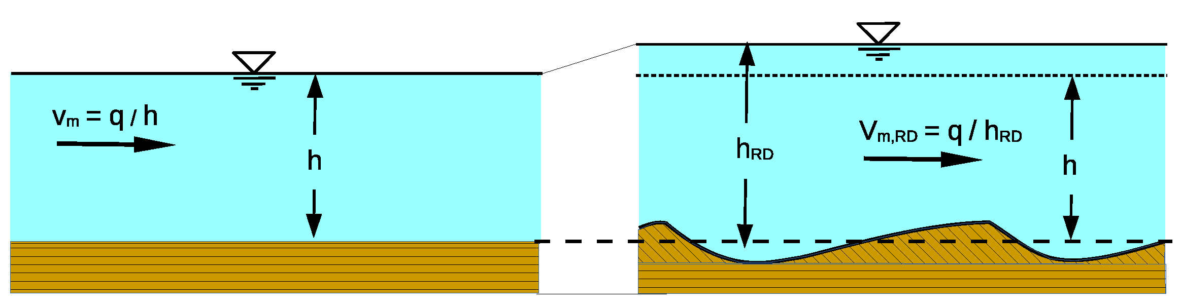
Morphodynamic processes in rivers and coastal areas can lead to many problems and considerable costs as a result of too much or too little sediment input. With a few exceptions, solutions for such problems can only be developed with morphodynamic models in which sediments move in mutual coupling with the local currents (e.g., Brakenhoff 2020 [1], Leone et al., 2021 [2]). As soon as ripples and/or dunes form on the sediment surface, these bedforms cause a specific flow resistance that influences the current and thus also the transport rates. In alluvial rivers, the flow velocity reduces when sand waves develop and the water depth increases (Figure 1).

The situation is different for tidal rivers, where the water level is controlled by the ocean tides. In this case, the water level cannot rise freely when ripples or dunes form, and thus not only the flow velocities but also the discharges are reduced by these bedforms. For this reason, models of morphodynamic processes require the prediction of form roughness due to bedforms. Since the first approaches in the 1930s, several such functions have been developed to calculate the form roughness in order to improve the quality of the results.

Relevant research has been published by, e.g., Motzfeld 1937 [3], Shinohara and Tsubaki 1959 [4], Ackers 1964 [5], Vanoni Hwang and 1967 [6], Swart 1967 [6], van Rijn 1982 [7], Höfer 1984 [8], Soulsby 1997 [9], Bartholdy et al., 2010 [10], Engelund and Hansen 1967 [11], Engelund 1977 [12], Vittal et al., 1977 [13], Lefebvre et al., 2016 [14] and Schippa et al., 2019 [15]. However, the structure and results of these approaches differ—in some cases, considerably. In order to arrive at a better understanding of this, our paper compares these approaches with a comparatively large amount of measurement data from different authors. The prediction of the presence and dimensions of ripples and dunes is a separate task that is not addressed here.

1.2. Tasks

In areas of fine and medium sand, ripples migrate. These bedforms occur regardless of the water depth with relatively short length L and small height H. The formation of ripples begins with sufficient sediment movement , i.e., $1<{\tau }^{★}/{\tau }_c^{★}<\approx 1.2$ (Liu 1957 [16]) where ${\tau }_c^{★}$ denotes the critical shear stress as introduced by Shields 1936 [17]. This is further restricted by $L^{★}=v^{★}L/\nu \approx$ 30,000, which corresponds quite well with the Yalin number $\chi =9$ (Zanke and Roland 2021 [18]).

The parameter $\chi =R{e}^{★}\sqrt{{\tau }^{★}}$ was introduced by Lapotre et al., 2017 [19]. Herein, $R{e}^{★}=v^{★}d/\nu$ and ${\tau }^{★}=v^{★2}/\left({\rho }^{\prime }gd\right)$, d = particle diameter, g = acceleration of gravity, $v^{★}$ = shear velocity, ${\rho }^{\prime }=({\rho }_s-\rho )/\rho$ = relative density with $\rho$ = density of fluid, ${\rho }_s$ = density of sediment, and $\nu$ = kinematic viscosity of the fluid. When $\chi >9$, dunes develop. Dunes on Earth occur in medium sand and coarser sediment. They reach heights up to approximately 30% of the water depth, h. Although much larger, dunes are not a priori rougher than ripples because their number per unit length is much smaller due to lengths of approximately $10<L/H<30$.

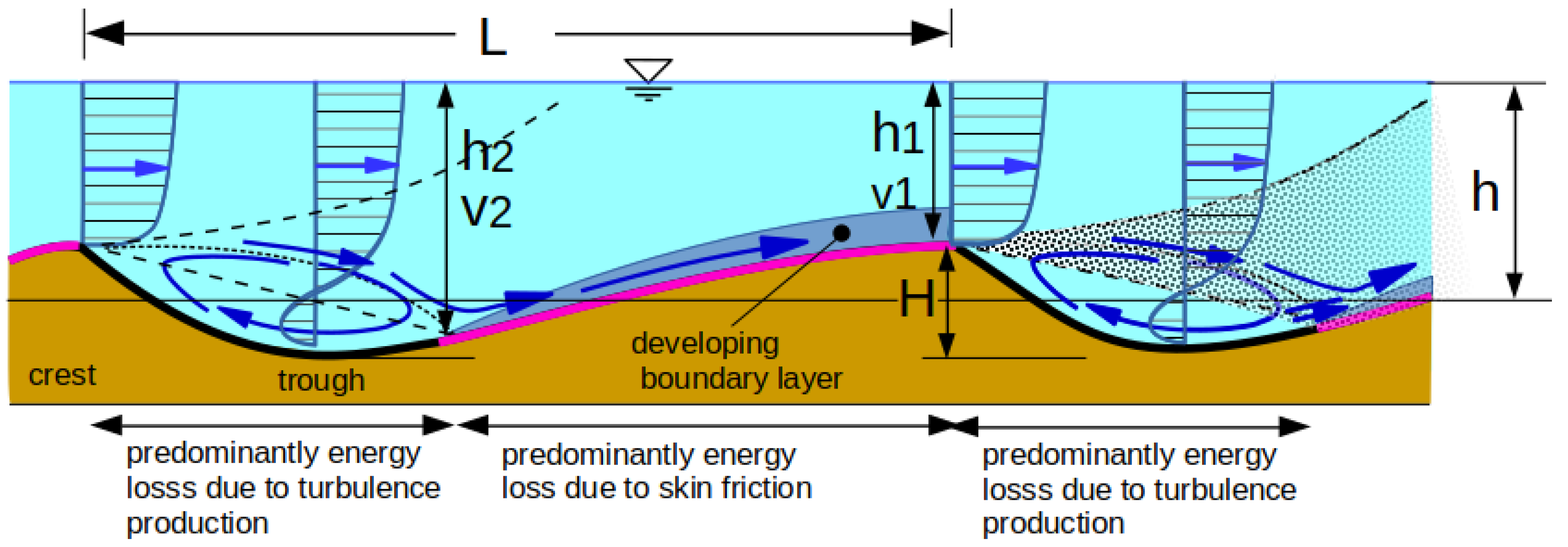
At the crest of the bed features, the flow separates, and a lee roller with a horizontal axis forms, which creates energy losses and, in this way, influences the flow regime. At the same time, the resistance due to skin friction in the area of the roller becomes largely subordinate. (See Figure 2). For bed load transport, the area of the stoss side with skin friction is largely effective.

Figure 1. The effects of bedforms on hydraulics (schematically).

Figure 1. The effects of bedforms on hydraulics (schematically).

Figure 2. Illustration of the areas with specific flow resistance over sand waves. Dotted lines indicate separation zones.

Figure 2. Illustration of the areas with specific flow resistance over sand waves. Dotted lines indicate separation zones.

Many approaches have been developed to predict the roughness of bedforms, such as ripples and dunes (see below in the tables, Table 1, Table 2 and Table 3). As early as 1937, Motzfeld [3] investigated energy losses through wavy walls at an early stage. He performed systematic experiments with different roughness types and developed a formula for calculating the roughness effect. Since then, a number of experiments have been conducted with this focus.

Semi-analytical functions were developed based on the definition of an effective roughness height of ripples and dunes, $k_{s,RD}$, and their transformation into a friction factor via the logarithmic velocity profile. Furthermore, semi-analytical functions based on Borda–Carnot’s expansion principle have been created as well as purely or widely empirical approaches.

However, the calculation of the form roughness is still comparatively fuzzy. The problem becomes apparent from the large number of solutions to the problem that have been proposed since then. The tasks of this paper are therefore

• a comprehensive comparison of the different approaches and
• the development of an improved prediction function.

2. Hydromechanical Relationships

The resistance of a sediment bed against the flow is generally described by the shear stress $\tau$ between the fluid and bed:

$$\tau =\frac{f}{8}\rho v_m^2=\rho v^{★2}$$

(1)

The resistance coefficient, f, thus, is

$$f=8{(v^{★}/v_m)}^2.$$

(2)

with $v_m=$ the time- and depth-averaged current velocity. For beds with sand waves, the total resistance is the sum of the resistance related to the bed features and the grain or skin resistance, which are described by the respective friction factors, i.e., grain-related shear stress $f_g$ and bedform-related stress $f_{RD}$. Grain-related resistance arises along the overflowing sediment surface, and form-related resistance arises from flow separations in the lee of the crests.

However, it is unphysical to define a total roughness height by simply adding the respective roughness heights to a total roughness height $k_S=k_{S,g}+k_{S,RD}$ and then calculating the total resistance $f_t$ with Equation (2) using Equation (8). The index “g” stands for the grain or skin roughness, and the index “$RD$” stands for the form roughness. Even if sometimes used this way, it remains a purely empirical procedure without a physical basis. In the case of ripples and dunes,

$${\tau }_t={\tau }_g+{\tau }_{RD}$$

(3)

$$f_t=f_g+f_{RD}$$

(4)

$${(v_m/v^{★})}_t={\left(\frac{1}{{(v_m/v^{★})}_g^2}+\frac{1}{{(v_m/v^{★})}_{RD}^2}\right)}^{-1/2}$$

(5)

The relationship between the average velocity and shear rate, $v_m/v^{★}$, is a measure of the flow resistance as expressed by Equation (2). For steady and uniform flow, $v_m/v^{★}$ can be determined by the assumption of a logarithmic velocity profile with

$$\frac{v_m}{v^{★}}=\frac{1}{\kappa }(ln\frac{h}{k_S}-1)+B$$

(6)

where $\kappa$ = the von Karman constant $\approx 0.4$ in undisturbed stationary flow, $k_S$ = equivalent sand roughness according to Nikuradse, $h=$ water depth and B an integration quantity. The latter depends on the type of flow, which may be hydraulically smooth, hydraulically rough or in a transition state and can approach natural roughness by

$$B=\frac{1}{\kappa }ln\frac{1}{0.033+0.11/R{e}^{★}}$$

(7)

with $R{e}^{★}=v^{★}{k}_S/\nu$ and $\nu =$ the kinematic viscosity of fluid. $k_S=a·d$ is the equivalent sand roughness after Nikuradse with a being a factor that is mostly chosen between 1 and 3. Here, we use $k_S=d$. Later, we investigate the effects of a and B on the results for bedform roughness.

Most approaches to bedform-induced friction in the literature for simplicity assume hydraulically rough conditions and therefore set $B=8.5$ when determining skin friction. Then, Equation (6) becomes

$$\frac{v_m}{v^{★}}=\frac{1}{\kappa }ln\left(11\frac{h}{k_S}\right)\mathrm{hydraulically}\mathrm{rough}\mathrm{only}.$$

(8)

3. Classes of Approaches for Determination of Bed Roughness

Figure 2 illustrates the areas of origin of specific losses of energy. Energy is lost on the one hand by wall friction due to grain roughness and on the other hand downstream of the crest due to flow separation. In the wake zone, energy is withdrawn from the flow through turbulent eddying. Starting at the point where the current reattaches to the bed, there is skin friction up to the crest.

The two roughness effects cannot be measured directly—only the total roughness effect. The form roughness is then obtained by subtracting the skin roughness, calculated, e.g., by Equations (2) and (6): $f_{RD,measured}=f_{measured}-f_{g,calculated}$. However, this can only be taken as an approximation wherefore the final result is inevitably imprecise. The main reason for this is that Equation (6) assumes a logarithmic velocity distribution profile and, strictly speaking, applies only to steady and uniform flows.

However, no such conditions exist along the part of the windward slope that generates skin friction. Therefore, a certain part of the uncertainties in the determination of the form-related roughness values is at the expense of the non-accurate determination of the skin roughness. However, the greater the proportion of form roughness in an individual case, the smaller this problem is and vice versa.

3.1. Determination of Skin Roughness

In the case of skin roughness, with the above discussed shortcomings, $f_g=8{(v^{★}/v_m)}^2$ can be determined from the logarithmic velocity profile. Traditional approaches to skin friction take the total length L of a bedform as decisive. However, skin friction occurs mainly on the slope $L_S$ (magenta in Figure 2). This simplification is also evaluated in the following.

3.2. Determination of Form Roughness

3.2.1. Determination via an Effective Bed Form Roughness Height and Length

This approach defines an effective roughness height of the bedforms. Clearly, the actual height of the sand waves, H, is important as well as the distance between the wake zones, i.e., L (Figure 2 and Figure 12). The associated hydraulically effective roughness height $k_{s,f}$ is thus a function of H and $H/L$. Equations (2) and (8) are then used to determine the friction coefficient $f_g$ assuming the validity of the logarithmic velocity profile.

3.2.2. Determination via the Borda–Carnot Loss Approach

Another approach is the direct computation of the energy loss downwind of the crests via the Borda–Carnot approach. Here, Equation (1) is used in combination with the Darcy–Weisbach approach of energy head loss, $h_v$:

$$h_v=f\frac{L}{4h}\frac{v_m^2}{2g}$$

(9)

or

$$f=\frac{8gh}{v_m^2}·\frac{h_v}{L}$$

(10)

with $L=$ any flow path, where the bedform length, $h_v/L=I_E=$ energy gradient and $g=$ the acceleration of gravity. Local losses, such as those downstream of a sand wave crest, can be determined with

$$h_v=\zeta \frac{v^2}{2g},$$

(11)

with $\zeta =$ energy loss coefficient. According to Borda–Carnot, the energy loss during a sudden widening of the flow, as it occurs after the stall at the crests, can be determined from the knowledge of the flow velocity and the cross-sectional areas before and after the widening. This approach is empirical but based on theoretical considerations. With the designations from Figure 2, the following can be written for the two-dimensional case with obstacles, such as ripples and dunes (RD)

$$h_{v,RD}=\frac{v_1^2}{2g}·{\left(1-\frac{h_1}{h_2}\right)}^2.$$

(12)

with $h_1\approx h-H/2$ and $h_2\approx h+H/2$. In the stationary case with $q=h_1{v}_1=h_2{v}_2=h{v}_m$ Equation (12) can be converted to

$$h_{v,RD}=\frac{v_m^2}{2g}{\left(\frac{1}{1-\frac{H}{2h}}-\frac{1}{1+\frac{H}{2h}}\right)}^2.$$

(13)

With the loss approach according to Darcy–Weisbach after Equation (9) yields

$$f_{RD}=4\frac{h}{L}{\left(\frac{1}{1-\frac{H}{2h}}-\frac{1}{1+\frac{H}{2h}}\right)}^2.$$

(14)

4. Approaches from the Literature

The approaches given in the literature can be divided into three groups:

4.1. Approaches via Empirical Determination of an Effective Form-Roughness Height

Many of these approaches are originally written in different notation. For better readability, the approaches were converted into a uniform notation as with that of Equation (8) without changing their physical content. Table 1 shows the key parameters $\kappa$ and $k_S/h$ of the individual approaches.

Table 1. Approaches via the logarithmic velocity profile (Equation (8)).

Author	Year	$\mathit{\kappa }$	$\frac{{\mathit{k}}_{\mathit{s},\mathbf{RD}}}{\mathit{h}}$
Motzfeld	1937 [3]	0.4	$10.3\frac{H}{h}\frac{H}{L}$
Shinohara and Tsubaki	1959 [4]	0.4	$7.5\frac{H}{h}{\left(\frac{H}{L}\right)}^{0.57}$
Ackers	1964 [5]	0.4	$37.7\frac{H}{h}{\left(\frac{H}{L}\right)}^{1.61}$
Vanoni and Hwang	1967 [6]	0.247	$55\frac{H}{h}\frac{H}{L}$
Swart	1967 [6]	0.4	$25\frac{H}{h}\frac{H}{L}$
van Rijn	1982 [7]	0.4	$1.1\frac{H}{h}\left(1-exp(-25\frac{H}{L})\right)$
Höfer	1984 [8]	0.4	$11.3\frac{H}{h}\frac{H}{L}$
Soulsby	1997 [9]	0.4	$27.5\frac{H}{h}\frac{H}{L}$
Bartholdy et al.	2010 [10]	0.4	$0.57\frac{H}{h}$

Table 1. Approaches via the logarithmic velocity profile (Equation (8)).

Author	Year	$\mathit{\kappa }$	$\frac{{\mathit{k}}_{\mathit{s},\mathbf{RD}}}{\mathit{h}}$
Motzfeld	1937 [3]	0.4	$10.3\frac{H}{h}\frac{H}{L}$
Shinohara and Tsubaki	1959 [4]	0.4	$7.5\frac{H}{h}{\left(\frac{H}{L}\right)}^{0.57}$
Ackers	1964 [5]	0.4	$37.7\frac{H}{h}{\left(\frac{H}{L}\right)}^{1.61}$
Vanoni and Hwang	1967 [6]	0.247	$55\frac{H}{h}\frac{H}{L}$
Swart	1967 [6]	0.4	$25\frac{H}{h}\frac{H}{L}$
van Rijn	1982 [7]	0.4	$1.1\frac{H}{h}\left(1-exp(-25\frac{H}{L})\right)$
Höfer	1984 [8]	0.4	$11.3\frac{H}{h}\frac{H}{L}$
Soulsby	1997 [9]	0.4	$27.5\frac{H}{h}\frac{H}{L}$
Bartholdy et al.	2010 [10]	0.4	$0.57\frac{H}{h}$

4.2. Approaches via Energy Loss at Sudden Widening (Borda–Carnot)

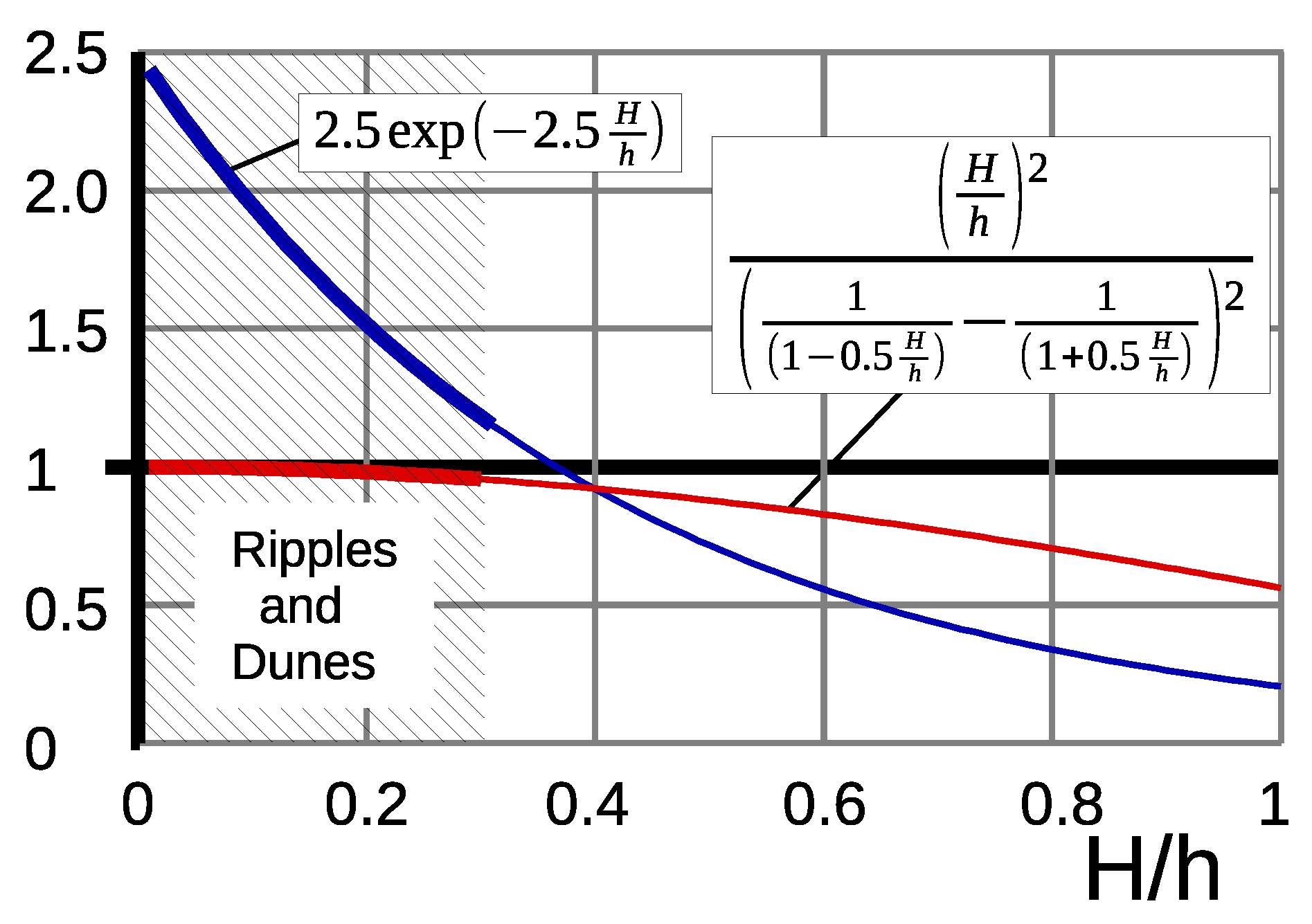
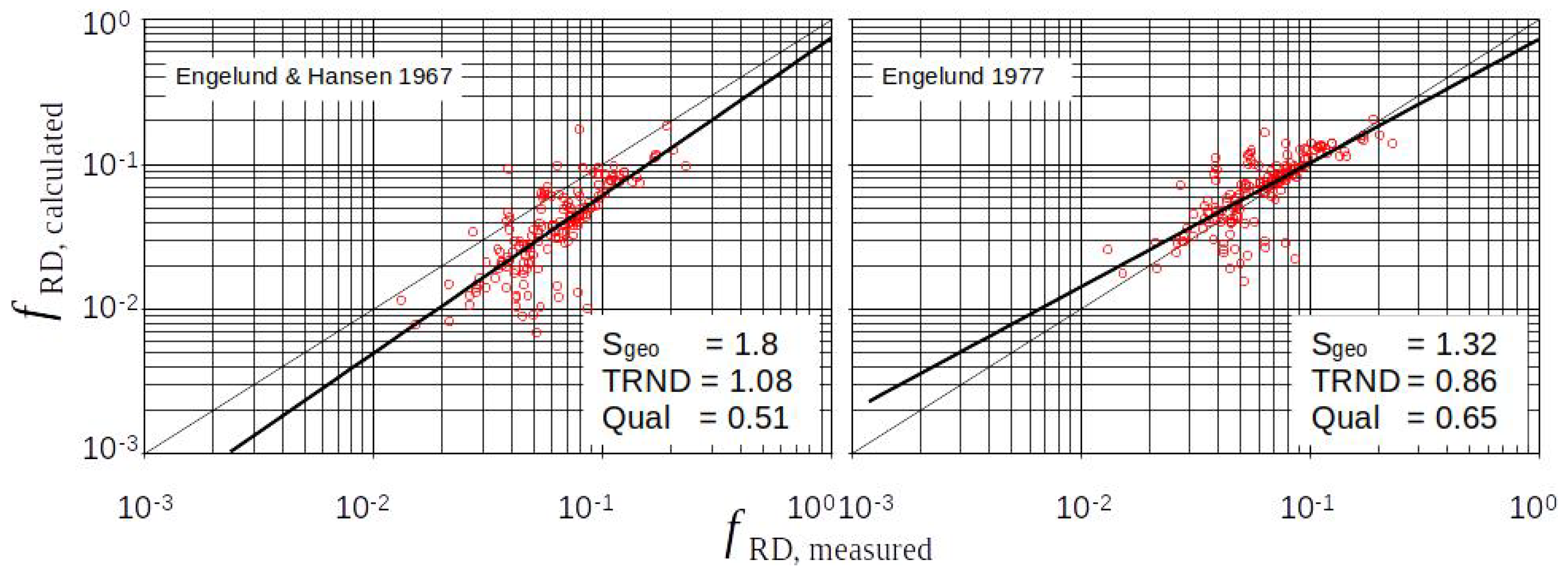
Two relevant approaches of this class are listed in Table 2. Engelund and Hansen 1967 [11], for simplification, replace the term in brackets from Equation (14) empirically by ${(H/h)}^2$ and, in this way they obtain

$$f_{RD}=4\frac{H}{h}\frac{H}{L}.$$

(15)

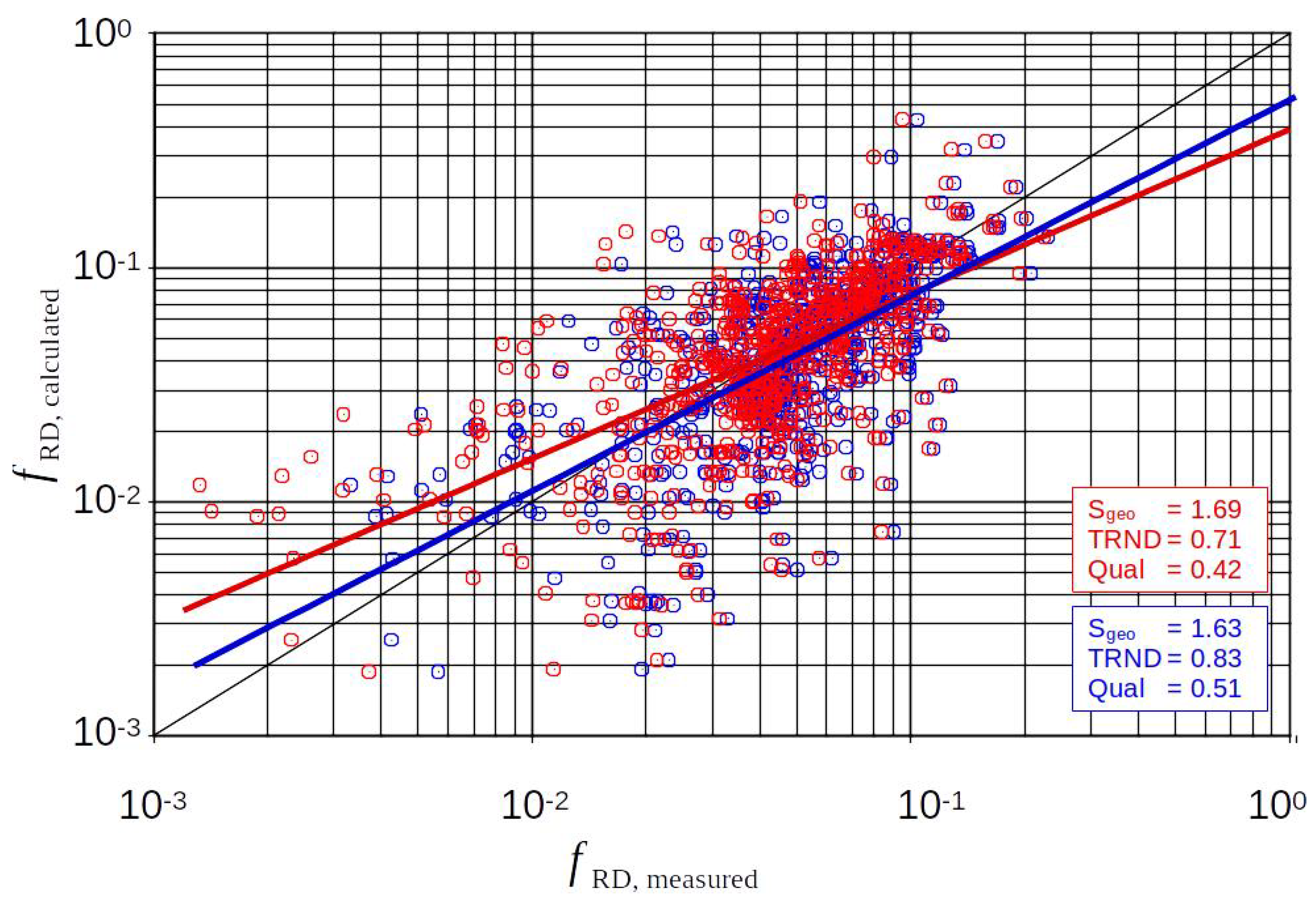
Figure 3 shows that this is acceptable within the typical range of natural bedforms, which is $H/h<\approx 0.3$.

By comparison with data, Engelund in 1977 [12] improved the quality of the evaluation of $f_{RD}$ by introducing the additional empirical term $2.5exp(-2.5H/h)$ (Table 2). The effects of this term are also shown in Figure 3. It reduces $f_{RD}$ with increasing relative roughness $H/h$.

Figure 3. Check of the effects of simplification of Equation (14) by Engelund and Hansen 1967 (red curve) and information on Engelund’s 1977 improvement term (blue) as functions of the relative roughness $H/h$.

Figure 3. Check of the effects of simplification of Equation (14) by Engelund and Hansen 1967 (red curve) and information on Engelund’s 1977 improvement term (blue) as functions of the relative roughness $H/h$.

Table 2. Approaches via Equation (14).

Author	Year	Friction Factor ${\mathit{f}}_{\mathbf{RD}}$
Engelund and Hansen	1967 [11]	$f_{RD}=4\frac{H}{h}\frac{H}{L}$
Engelund	1977 [12]	$f_{RD}=4\frac{H}{h}\frac{H}{L}\left(2.5exp(-2.5\frac{H}{h})\right)$

Table 2. Approaches via Equation (14).

Author	Year	Friction Factor ${\mathit{f}}_{\mathbf{RD}}$
Engelund and Hansen	1967 [11]	$f_{RD}=4\frac{H}{h}\frac{H}{L}$
Engelund	1977 [12]	$f_{RD}=4\frac{H}{h}\frac{H}{L}\left(2.5exp(-2.5\frac{H}{h})\right)$

4.3. Empirical Approaches

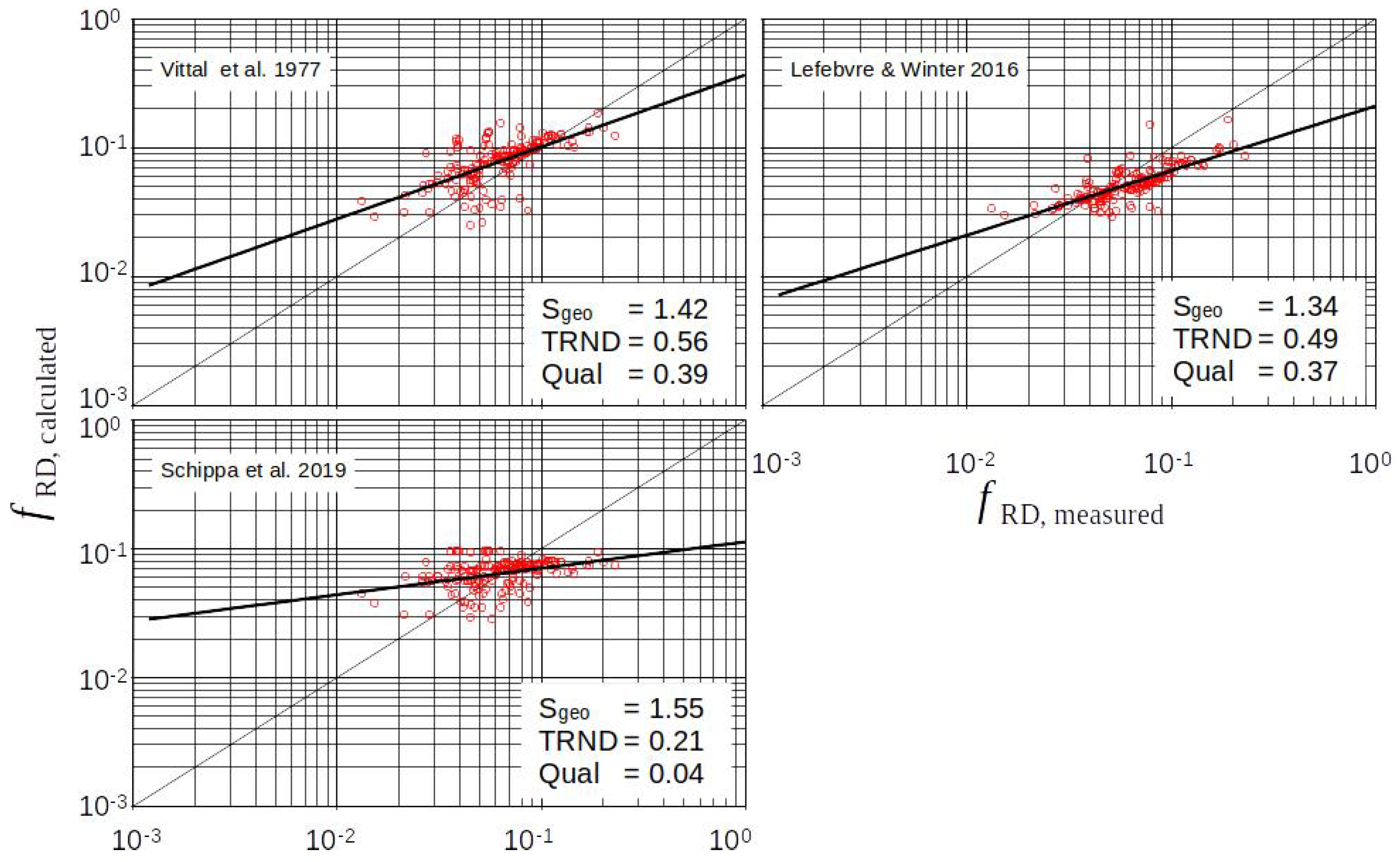
In addition, there are entirely or largely empirical approaches based less on physical considerations and instead on curve fitting.

Table 3. Empirical approaches for $f_{RD}$.

Author	Year	Formula
Vittal et al. *	1977 [13]	$f_{RD}=4m{\left(\frac{H}{h}\right)}^{3/8}\frac{H}{L}$
Lefebvre et al.	2016 [14]	$f_{RD}={\left[8.5ln\left(\frac{hL}{10.61H^2}\right)\right]}^{-1}$
Schippa et al.	2019 [15]	$f_{RD}=0.56\frac{{\left(\frac{H}{L}\right)}^{0.81}}{{\left(1-(\frac{1}{2}\frac{H}{h}{)}^2\right)}^2}$

* Vittal et al. gave the coefficient $m$ in in tabular form. It ranged from $0.46$ to $0.53$ for $20>L/H>10$. Here, $m$ is set at 0.5, which causes an error for $f_{RD}$ of a maximum of $\approx$ 10%.

Table 3. Empirical approaches for $f_{RD}$.

Author	Year	Formula
Vittal et al. *	1977 [13]	$f_{RD}=4m{\left(\frac{H}{h}\right)}^{3/8}\frac{H}{L}$
Lefebvre et al.	2016 [14]	$f_{RD}={\left[8.5ln\left(\frac{hL}{10.61H^2}\right)\right]}^{-1}$
Schippa et al.	2019 [15]	$f_{RD}=0.56\frac{{\left(\frac{H}{L}\right)}^{0.81}}{{\left(1-(\frac{1}{2}\frac{H}{h}{)}^2\right)}^2}$

* Vittal et al. gave the coefficient $m$ in in tabular form. It ranged from $0.46$ to $0.53$ for $20>L/H>10$. Here, $m$ is set at 0.5, which causes an error for $f_{RD}$ of a maximum of $\approx$ 10%.

Note that the approach of Schippa et al. starts from the Borda–Carnot principle but is classified as empirical here because it includes major empirical extensions. This results in a different quality with respect to the ripples on one side and the dunes on the other side as can be seen further below from the Figure 7 and Figure 10.

4.4. Intermediate Evaluation

In comparing the first two approaches, it is noticeable that the same quantity $\frac{H}{h}\frac{H}{L}$ in the approaches of Table 1 describes a roughness height where, for those in Table 2, they directly represent the form resistance. This suggests the conclusion that, if at all, only one of the two approaches may apply in a physical sense.

5. Comparison of the Approaches versus Data

5.1. Data

A set of 637 measurements, from laboratory experiments and nature, was used to compare the approaches according to Table 1, Table 2 and Table 3. These data are described by

Table 4. The main characteristics of the comparative data.

Author(s)	Year	Lab./Nature	Water Depth h (m)	Number of Data
Shinohara and Tsubaki	1959 [4]	Hii-River	$0.1<h<1$	36
Stein	1965 [20]	Lab	$0.12<h<0.31$	17
Simons and Richardson	1966 [21]	Lab	$0.06<h<1.06$	163
Vanoni and Hwang	1967 [6]	Lab	$0.07<h<0.29$	22
Stückrath	1969 [22]	Rio Parana	$\approx 12$	1
Zanke	1977 [*]	Lab	$0.37<h<0.92$	4
Grazer	1982 [23]	Lab	$0.047<h<0.127$	6
Engel and Lau	1980 [24]	Lab	$0.07<h<0.3$	37
Höfer	1984 [8]	Lab	$0.09<h<0.4$	55
Hong, Karim and Kennedy	1984 [25]	Lab	$\approx 0.07$	19
Klaassen	1992 [26]	Lab	$0.09<h<0.4$	14
Julien	1992 [27]	Missouri	$2.8<h<5$	23
Julien	1992 [27]	Rio Parana	$22<h<26$	13
Julien	1992 [27]	Jamuna	$8.2<h<18.6$	33
Julien	1992 [27]	Zaire River	$9.5<h<17.6$	21
Julien	1992 [27]	Maas	$6.2<h<10.50$	26
Julien	1992 [27]	Meuse	$6.8<h<9.52$	60
Kühlborn	1993 [28]	Lab	$0.084<h<0.185$	39
Gaweesh and v. Rijn	1994 [29]	River Nile	$3.9<h<5.7$	6
Gaweesh and v. Rijn	1994 [29]	River Rhein	$4.8<h<6.1$	4
Gaweesh and v. Rijn	1994 [29]	Lab	$0.37<h<0.5$	9
Wallisch	1996 [30]	Lab	$0.15$	1
Wieprecht	2001 [31]	Lab	$0.08<h<0.5$	29

[*] unpublished data 637.

,

Table 5. The main characteristics of the comparative data (all data).

	d	h	H	L	H/L	H/h	h/d	Fr	I	$\mathit{\chi }$
	mm	m	m	m	-	-	-	-	-	-
min.	0.02	0.047	0.006	0.09	0.0012	0.023	19.6	0.07	$6·{10}^{-7}$	0.26
max.	90	26	7.5	735	0.22	0.83	97500	1.2	0.0032	146

and

Table 6. The main characteristics of the comparative (data qualified as ripples).

	d	h	H	L	H/L	H/h	h/d	Fr	I	$\mathit{\chi }$
	mm	m	m	m	-	-	-	-	-	-
min.	0.02	0.047	0.006	0.09	0.033	0.023	133	0.04	6.6 · 10${}^{-5}$	0.26
max.	0.7	0.5	0.51	0.6	0.155	0.455	6200	0.77	0.0043	9

.

5.2. “Measured” Form Roughness

The measurement results initially provide the total roughness or resistance by the sum of skin friction and form resistance. Form resistance values are then derived by subtracting the calculated skin roughness from total roughness. This means that the “measured” form roughness values (from here denoted by ”) are not directly measured but are calculated—and to a certain degree falsified by—the somewhat fuzzy determination of the skin roughness.

In the following, the accuracy for the friction coefficient $f_{RD}$ was separately determined in the case of ripples and for all data (ripples and dunes). This is due to the fact that the measured values of $H,L,d$ and bed inclination I are generally more accurate for ripple beds than for dunes, especially if they come from measurements in the laboratory, as is mostly the case here:

• In a measured section, there are generally many more ripples than dunes.
• According to various observations, including those of Zanke 1976 [32], the variation of the dune parameters H and L from one dune to the next is often considerable. Echograms from the Rio Parana of Stückrath 1969 [22] show, e.g., differences in H of about 60% and in L of about a factor of 2 for dunes following each other directly.
• The determination of the sediment grain size is more accurate for ripples than for dunes, because typically several ripples are captured during sampling, while for dunes, the sediment determination is much more uncertain.

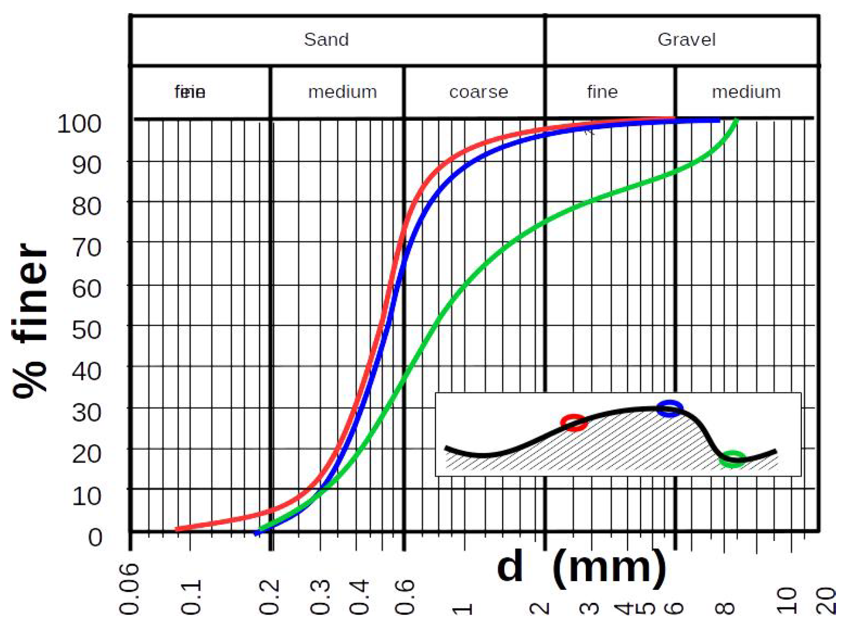
Samples taken by Vollmers and Wolf 1969 [33] at dunes in the Lower Elbe River in Northern Germany (Figure 4) clearly illustrate this. Nasner (1974) [34] produced comparable results in samples taken in the Lower Weser River. The sediment is clearly and systematically finer in the crest region than in the troughs. In particular, when measuring in nature, only drill cores from the crest area of dunes can give reliable information about the sediment in a dune field. However, this is usually not the case for measurements in nature. Locally random soil samples can therefore lead to appreciable misinterpretations of the transported material.

5.3. Comparison of the Approaches from Tables 1–3 to the Data from Table 4

5.3.1. Case 1: Ripples

According to Zanke and Roland 2021 [18], ripples are indicated by a Yalin-number $\chi =R{e}^{★}\sqrt{{\tau }^{★}}<9$. Variously in the literature, $L<0.6$ m for ripples is also specified, e.g., Flemming 1988 [35] and Ashley 1990 [36]. Different stability diagrams show the ripple domain (e.g., Zanke 1976 [32], Southard and Boguchwal 1990 [37], van den Berg and van Gelder 1993 [38]). Here, 154 data points of Table 4 are specified as ripples with the criteria $\chi <9$ and $L<0.6$ m.

Approaches via the Logarithmic Velocity Profile

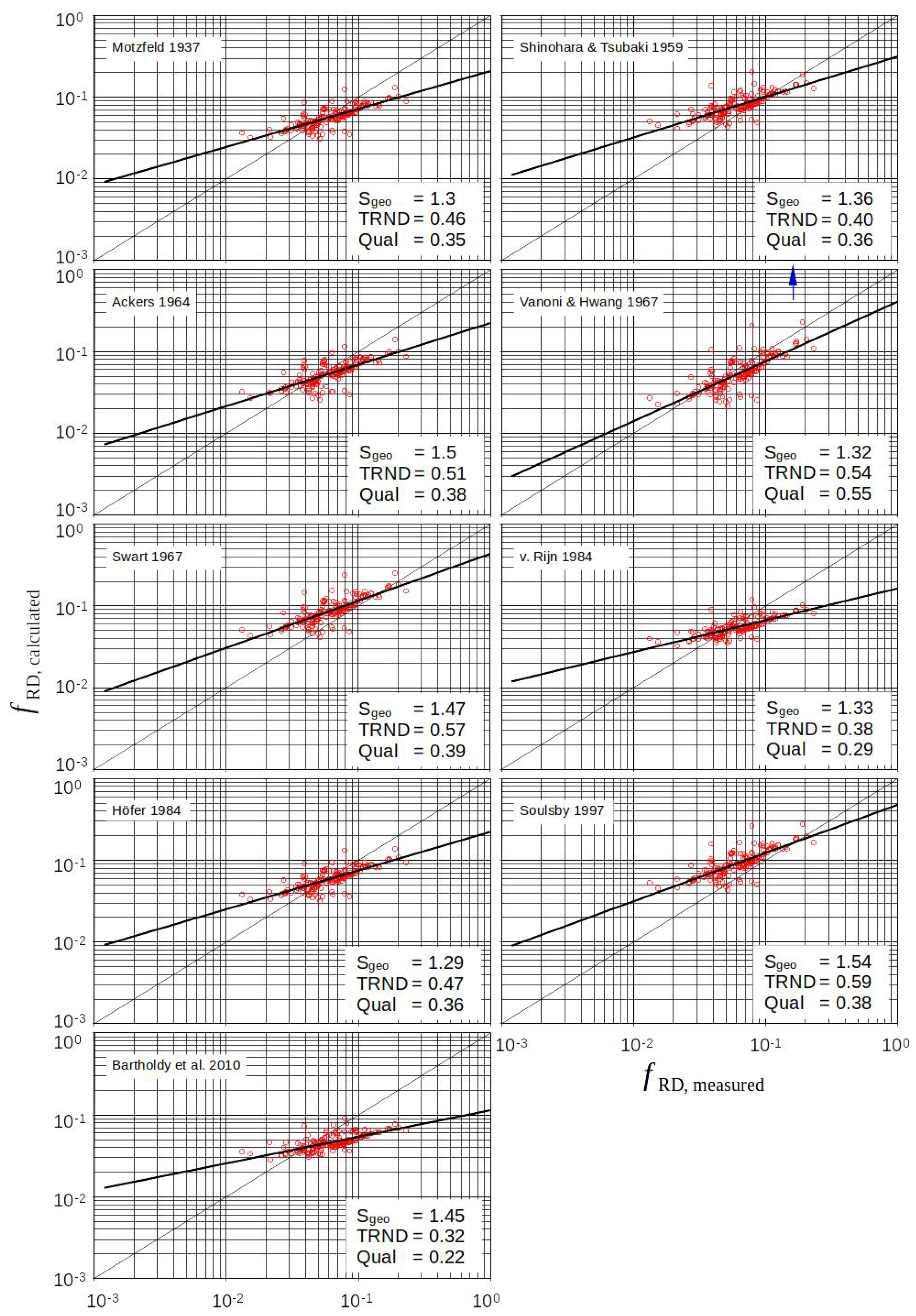
Figure 5 shows the quality of the different approaches for only ripples. The trend curves of the individual solutions were calculated by regression functions of the form $y=a{x}^b$. For the nine approaches tested in this class, there is a clear trend toward overestimation of the roughness effect for small form roughness and underestimation for large form roughness. Another difference between the approaches is the absolute magnitude of the roughness effect.

Only the approach of Vanoni and Hwang 1967 [6] provided a better trend. This is clearly due to the empirically determined values of $\kappa =0.247$ in Equation (6), which result from a transcription of their original notation $f_{RD}={(3.3lg(hL/H^2)-2.3)}^{-2}$. Since the velocity profile over ripples and even more over dunes is constantly changing along the flow path, its description by the profile for steady and uniform flow given by Equation (6) with the values for $\kappa =0.4$ is only a rough approach.

Figure 5. Approaches via the log profile $f_{RD}=8{(v/v^{★})}^{-2}$ and Equation (8) in the case of ripples.

Figure 5. Approaches via the log profile $f_{RD}=8{(v/v^{★})}^{-2}$ and Equation (8) in the case of ripples.

Approaches via Borda–Carnot Expansion Law

Figure 6 shows that this approach, as used by Engelund and Hansen 1967 and Engelund 1977, provides significantly better results than the approaches via the velocity profile.

Purely or Widely Empirical Approaches

From Figure 7, it becomes clear that completely or largely empirical approaches have no advantage. Due to a lack of physics, they always suffer from the fact that they react problematically to data sets that go beyond the data available for calibration. A further problem is the impossibility to causally analyze individual effects.

Figure 7. Purely ore widely empirical approaches in the case of ripples.

Figure 7. Purely ore widely empirical approaches in the case of ripples.

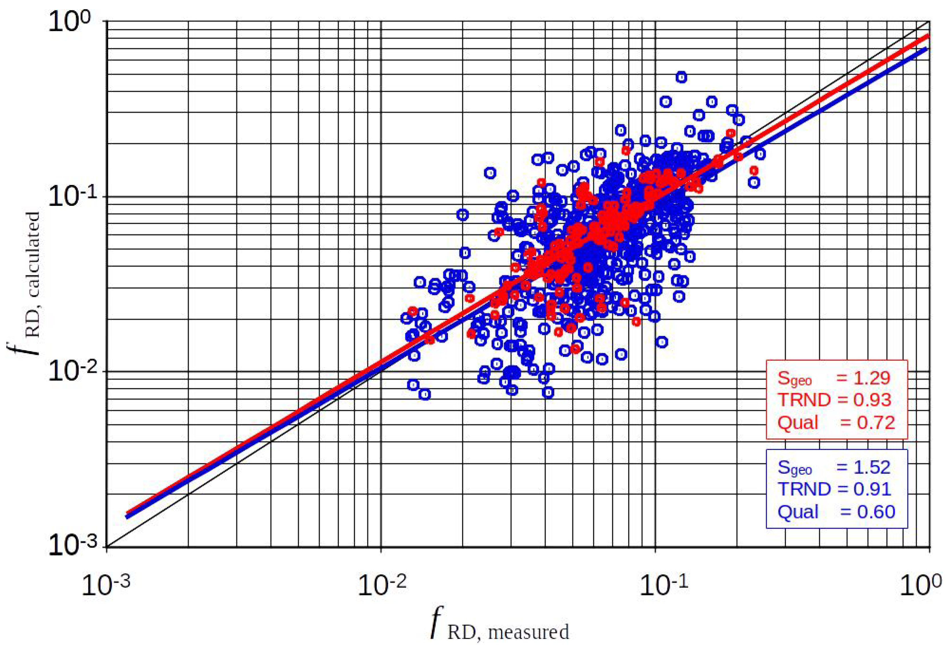
5.3.2. Case 2: Ripples and Dunes

Approaches via the Logarithmic Velocity Profile

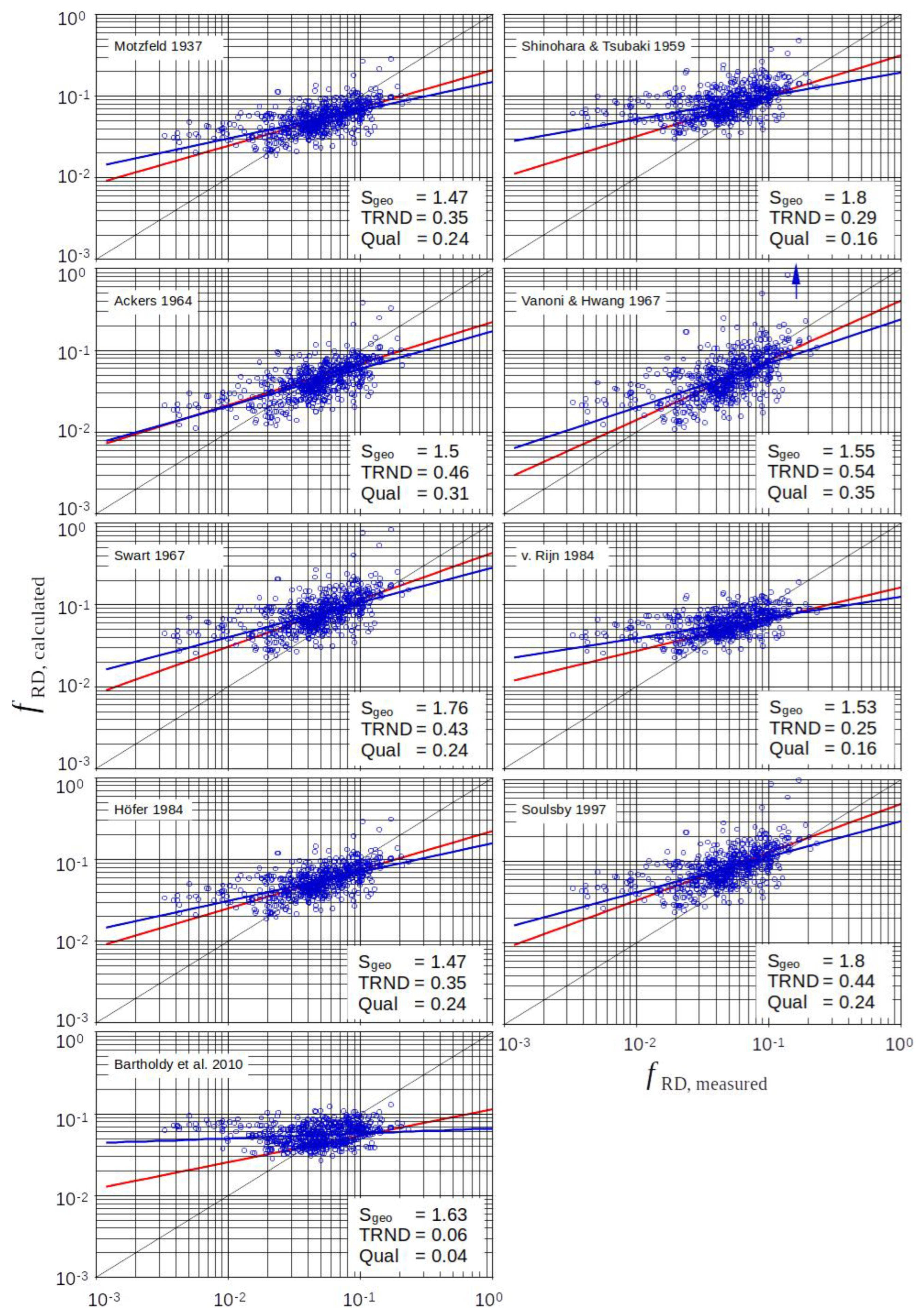
Figure 8 demonstrates the performance of the various approaches for 637 cases of ripples and dunes. For the nine tested approaches, which are based on the logarithmic velocity profile, the general trend and the specific error is similar (but most of the time slightly worse) to the case of only ripples.

The approach of Vanoni and Hwang 1967 [6] with a modification of $\kappa$ in Equation (6) again delivers the best results in this class with respect to the general trend. However, there are some calculated results outside the grid.

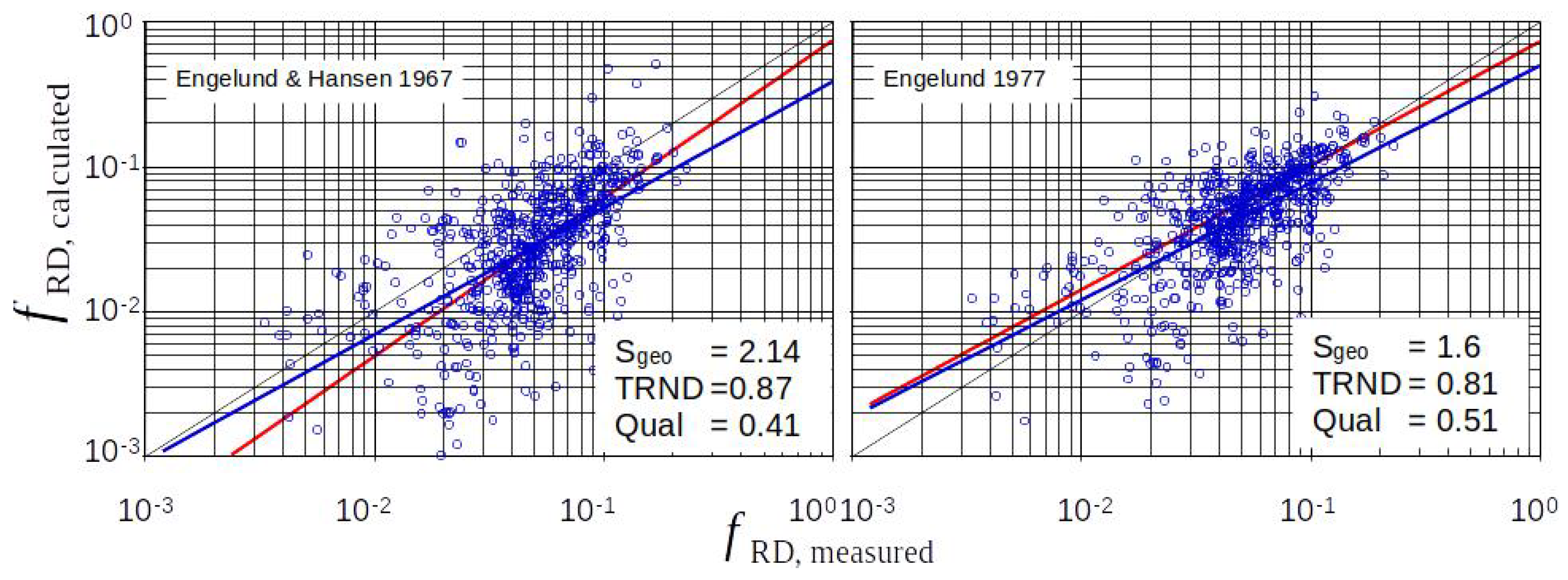
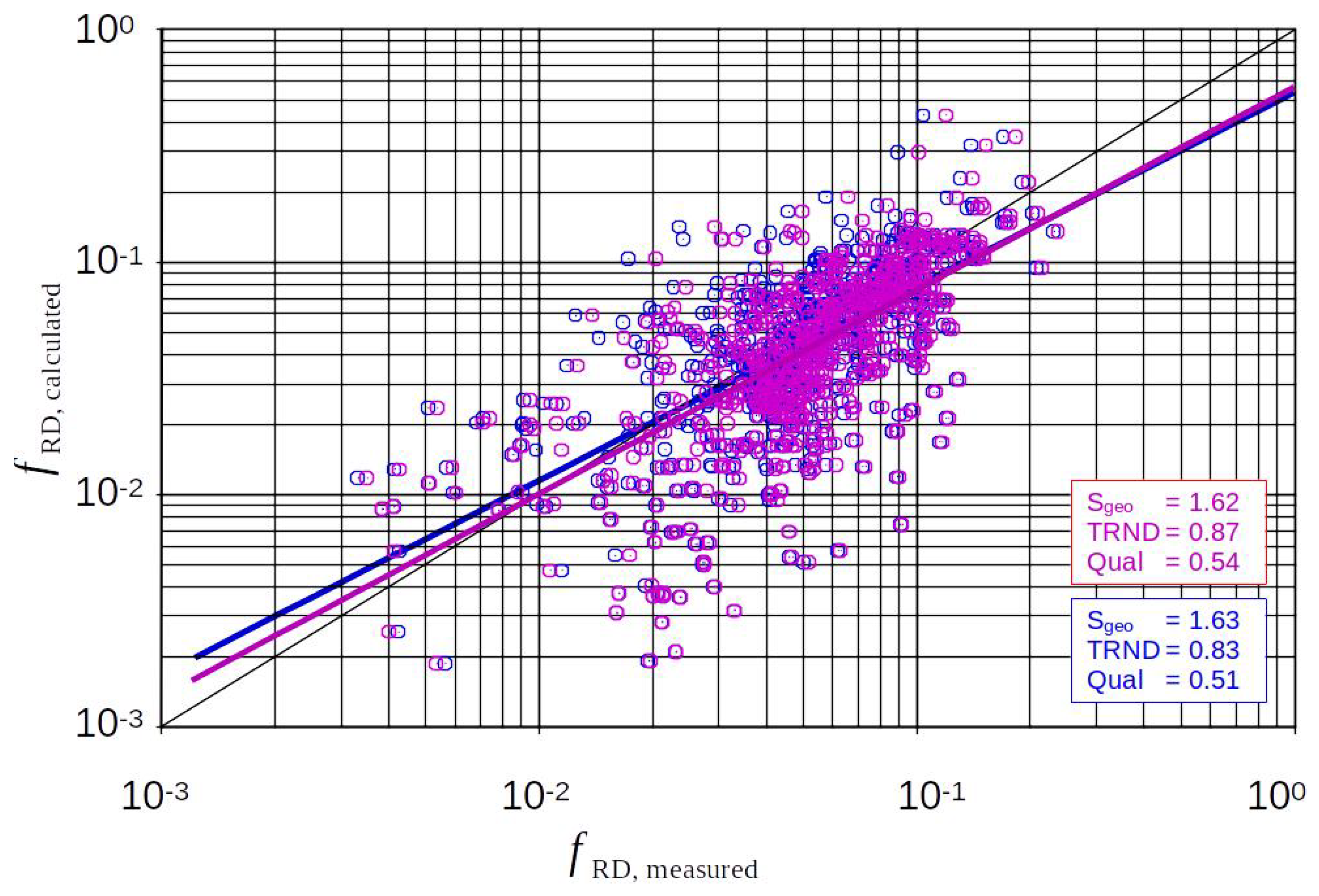
Approaches via the Borda–Carnot Expansion Law

With respect to the general trend, Figure 9 shows that the solution via the Borda–Carnot expansion loss describes the physics the better than the other approaches. The Engelund 1977 solution again provides the best results.

Purely or Widely Empirical Approaches

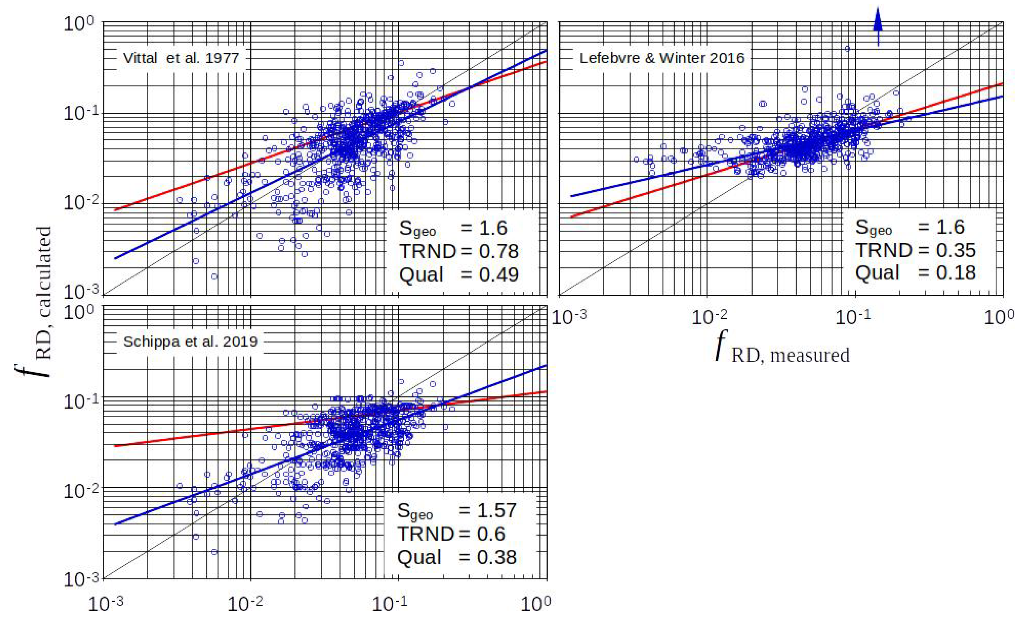
From Figure 10, for dunes it also becomes clear that completely or largely empirical approaches do not bring an advantage. Not untypical is a divergent trend in the results for ripples on the one hand and for dunes on the other hand (trendline ripples (red) and all data (blue) may diverge significantly as in Vittal 1977 [13] or Schippa 2019 [15]). In the case of Lefebvre et al. 2016 [14], it is important to note that the trend curves for the 154 ripple data and the 637 data for ripples and dunes show only slight deviations with respect to their trend. However, the trend deviates strongly from the line $f_{calc}=f_{meas}$. It can also be concluded that the approaches of Vittal and Schippa show improved trends when the data set with dunes is considered as Figure 10 indicates.

5.3.3. Quality Characteristics

On the one hand, the quality of the different approaches can be evaluated visually. On the other hand, the results can be rated via characteristic values. One such characteristic value is the geometrical standard deviation, $s_{geo}$, which is the average multiple of the forecast versus the measured value:

$$s_{geo}={\left(Product{\left(r_i\right)}_{i=1}^{i=n}\right)}^{1/n}$$

(16)

with $r=\frac{f_{RD,calc}}{f_{RD,meas}}$ and $r=1/r$ in the case of $r<1$. In this way, $S_{geo}$ describes the deviation to both sides of perfect results, which fall on the diagonal in a plot ’calculated = f(measured)’. The closer $S_{geo}$ is to 1, the better the rated formula.

Another feature is the exponent of the power regression (PR) functions of $f_{RD,calc}=f\left(f_{RD,meas}\right)$. In the case of perfect agreement between measurement and calculation, the exponent $ex=1$. Measurements, however, will typically show $ex\ne 1$. The deviation from the perfect trend can be described by the qualifier $TRND=e{x}_{PR}/e{x}_{perfect}$. In the case of exponents $e{x}_{PR}>1$, $1/e{x}_{PR}$ is to be used. In this way, the qualifier for the trend is always $TRND<=1$.

We combine both qualifiers to describe the quality of the respective results by

$$Qual=\frac{TRND}{S_{geo}}.$$

Figure 10. Purely or widely empirical approaches in the case of ripples and dunes (red trendline: ripples, blue trendline: all data, and blue arrow = some results outside).

Figure 10. Purely or widely empirical approaches in the case of ripples and dunes (red trendline: ripples, blue trendline: all data, and blue arrow = some results outside).

6. Approaches to Further Improve the Quality of Forecasts

The above results show, especially with respect to the trend, that an approach based on Borda–Carnot’s expansion loss law describes the form roughness effect better than the other two classes of approaches. In the following, we therefore focus on Engelund and Hansen’s 1967 basic approach and investigate possibilities to further improve it.

6.1. Regarding the Effects of Relative Water Coverage, $h/H$

The traditional descriptions of hydraulic resistance in open channels are valid only when the depth h is much greater than the roughness height $k_S$. If the relative coverage becomes smaller than about $h/k_S\approx 100$, turbulence damping occurs (e.g., v. Driest 1956 [39], Nezu and Rodi 1986 [40] and Nezu and Nakagawa 1993 [41]). The resistance of flow obstacles then becomes smaller, and a change in the velocity profiles occurs.

From $h/k_S\approx$ 100 and below, this effect begins and becomes clearly evident in practice when approximately $h/k_S<10$. In the case of dunes, the magnitudes of $h/H$ are usually well below $h/H\approx 10$. In the case of ripples, $h/H>10$ is often the situation in nature. However, many laboratory experiments with ripples were performed with shallow water depth at $h/H<10$. The above descriptions of hydraulic resistance in open channels are therefore incomplete as soon as the effect of low water cover becomes noticeable, i.e., when $h/H<\approx 10$.

Based on work by Nezu and Rodi [40], Zanke 2001 [42] and Zanke 2003 [43] proposed turbulence damping:

$$\frac{v_{rms,b}^{\prime }}{v^{★}}=0.31k_S^{+}·ex(-0.1k_S^{+})+1.8·exp(-0.88\frac{k_S}{h})·(1-exp(-0.1k_S^{+})).$$

(17)

with $v_{rms,b}^{\prime }$ the rms of the turbulent fluctuation velocity at the bed, $k_S^{+}=R{e}^{*}{k}_S/d$ and $R{e}^{★}=v^{★}d/\nu$. Here, $k_S/h$ is replaced by $H/h$. As a first approach, the flow conditions in the lee of the crests can be treated as fully turbulent. Then, Equation (17) simplifies to

$$\frac{v_{rms,b}^{\prime }}{v^{★}}=1.8·exp(-0.88\frac{H}{h}).$$

(18)

Strictly speaking, the effective shear stress is determined not only by the mean value of $\overline{\tau }$ (which is mostly simplifying written as $\tau$) but also by the distribution of turbulent shear peaks ${\tau }^{\prime }$. If ${\tau }^{\prime }$ is dampened, the same $\overline{\tau }$ would be less effective compared to a case with fluctuations as the strongest ${\tau }^{\prime }$ are most effective. For this reason, the bedload movement, e.g., at low coverage, begins only at an increased value of the critical shear stress $\overline{{\tau }_c}$. This is why the bandwidth of ${\tau }^{\prime }$ decreases.

The effects of this can be described by a damping coefficient, $D_{\tau }$, which, in the case of low relative coverage can be calculated by (indices $h/H$ indicate values in the range of influence of low water coverage)

$$D_{\tau }=\frac{{\tau }_{h/H}}{\tau }=\frac{f_{h/H}}{f}={\left(\frac{{(\frac{v_{rms,b}^{\prime }}{v^{★}})}_{h/H}}{{(\frac{v_{rms,b}^{\prime }}{v^{★}})}_{h/H>100}}\right)}^2$$

(19)

i.e., with Equation (17)

$$D_{\tau }={\left(\frac{0.31k_S^{+}·e^{-0.1k_S^{+}}+1.8·e^{-0.88\frac{d}{h}}·(1-e^{-0.1k_S^{+}})}{0.31k_S^{+}·e^{-0.1k_S^{+}}+1.8·1·(1-e^{-0.1k_S^{+}})}\right)}^2,$$

(20)

and, in the fully turbulent case, this reduces to

$$D_{\tau }=e^{-1.76\frac{H}{h}}.$$

(21)

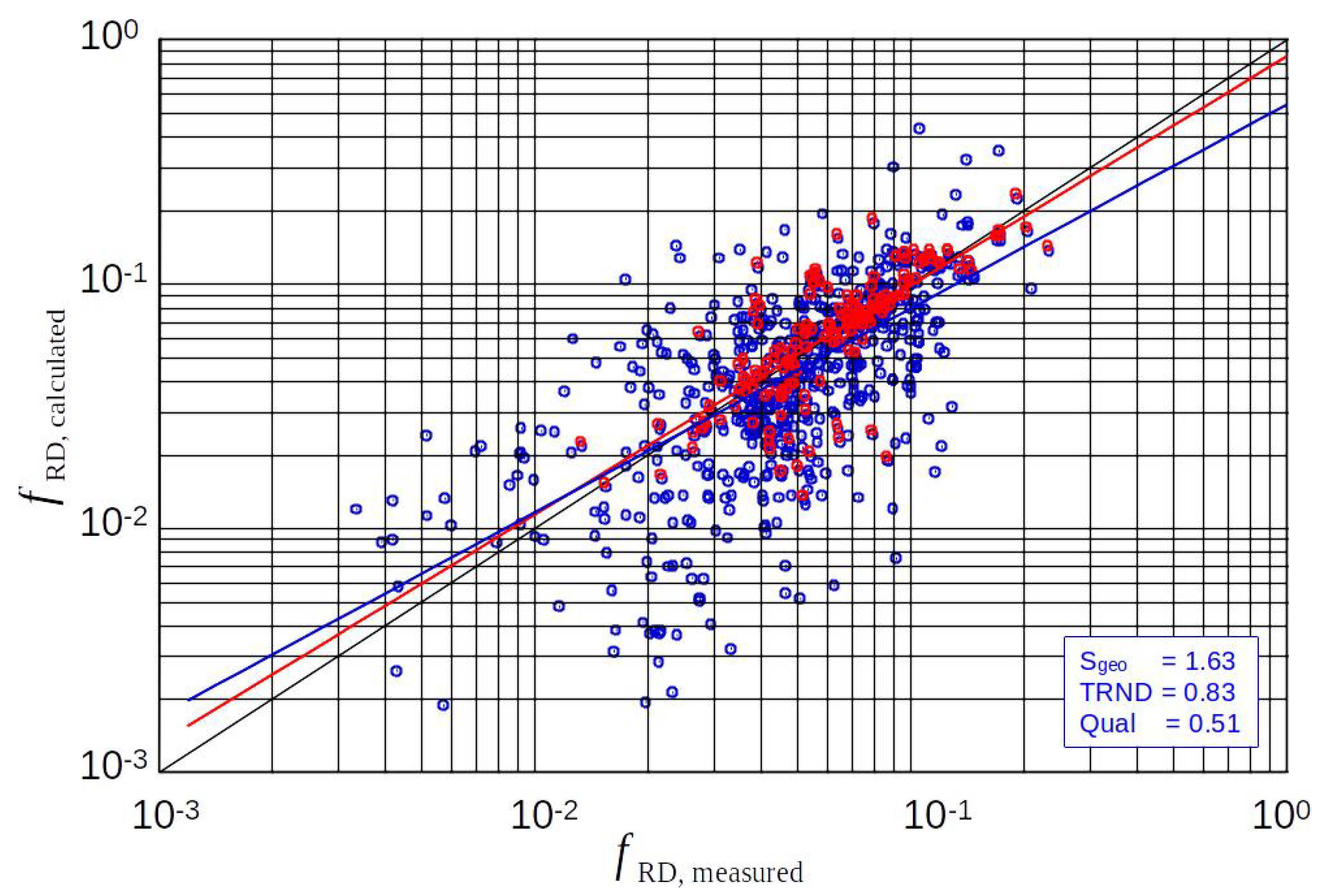
Based on the above described background, the drag coefficient can be improved to

$$f_{RD}=4\frac{H}{h}\frac{H}{L}\left(2.12exp(-1.76\frac{H}{h})\right).$$

(22)

Figure 11 shows the results for the ripple data (red) and all data (blue). In the final effect, Equation (22) it is largely congruent with the solution of Engelund 1977 (Table 2 and Figure 9). This explains the physical background, why the empirical term, which Engelund introduced in 1977 into the equation of Engelund and Hansen 1967 (see Table 2), brought considerable improvements. Although empirical, Engelund’s additional term fits the effects of turbulence damping in the case of low water coverage quite well. The trend curves for ripples and for ripples and dunes hardly deviate from each other and are close to the target values $f_{calc}=f_{meas}$.

Based on Equation (22), the geometric standard deviation $s_{geo}$ for the calculated vs. measured friction factors $f_{RD}$ is evaluated. For the ripples only dataset, a value of $s_{geo}=1.29$ was obtained based on the data of Table 4. This means that the calculation yields, on average, between $1.29$-times too large or $1/1.29$-times too small results. For all 637 data with ripples and dunes, $s_{geo}=1.63$. The larger scatter in the case with dunes is likely due to inaccurate measurement results as mentioned above.

6.2. Enhancements with Respect to the “Measured” Form Roughness

The following investigations were conducted based on Equation (22).

6.2.1. Regarding the Flow Path with Effective Skin Friction

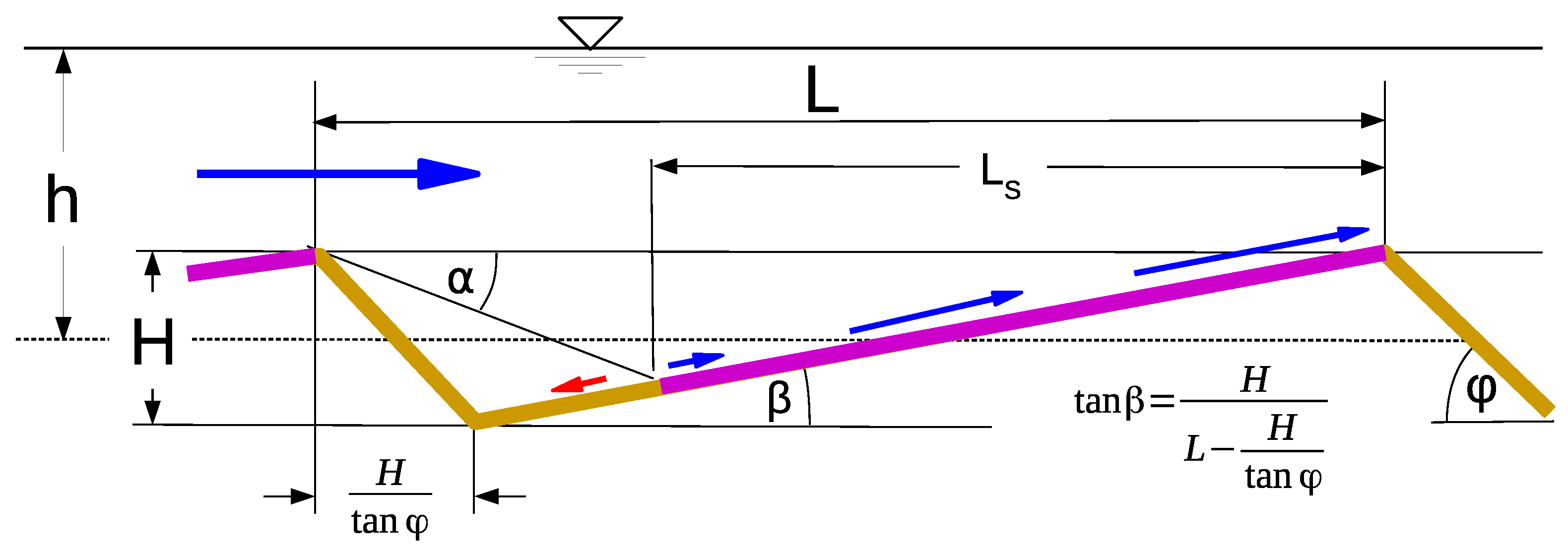
One uncertainty in the relationship “calculated vs. measured” form roughness results from the determination of the “measured” form roughness on the flow path, which is taken as significant for skin friction. This flow path is usually assumed as the total sand wave length L. However, skin friction mainly takes place on the windward slope of ripples and dunes, which is marked by $L_S$ in Figure 12 in magenta. To determine the effects of this, the profile of the ripples and dunes is approximated by triangular shapes. This results in

$$(L-L_S)tan\alpha =L_{S}tan\beta$$

(23)

or

$$\frac{L_S}{L}=\frac{1}{\frac{tan\beta }{tan\alpha }+1}$$

(24)

and

$$tan\beta =\frac{1}{\frac{L}{H}-tan\phi }.$$

(25)

Herein, $\phi$ is the angle of repose, which ranges around approximately ${30}^{\circ }$. Sometimes the lee angle of the dunes is smaller than even ${20}^{\circ }$. Then, the respective friction factor is reduced, which can be taken into account by an approach of Lefebvre and Winter 2016 [14]. Regarding this, the skin friction is reduced by a factor of $L_s/L$.

Figure 12. Definitions.

Figure 12. Definitions.

As a result, the length considered effective for skin friction, L or $L_s$, proved to be marginal compared to the remaining spread. This is shown in Figure 13.

6.2.2. Influence of the Choice of $k_S/d$ on the “Measured” Friction Factor

Next, we investigated the effects of the choice of $k_S/d$ on $f_{RD,meas.}$. Typically, $1<k_S/d<3$ is chosen in the literature.

The investigation of the effects of the choice of $k_S/d$ showed noticeable effects only with small form roughness (and correspondingly dominant grain roughness) as can be seen in Figure 14. With larger $k_S/d$, the grain roughness increases and thus the “measured” form roughness is expected to be slightly reduced.

6.2.3. Skin Friction Assumed as Active on Full Length of the Ripples and Dunes and B Determined by Iteration

In case of dunes with low steepness $H/L$, the proportion of grain roughness (=skin roughness) is significantly higher than that of ripples. For this reason, and because roughness conditions in the hydraulic transition region may occur, the integration constant B of the logarithmic velocity distribution law should be determined by iteration when determining the “measured” grain roughness, rather than simply assuming $B=8.5$.

The investigation of this influence revealed noticeable effects. For small total roughnesses, lower skin roughness values were calculated with the consequence of larger calculated “measured values” of the form roughness. Figure 15 shows the result. Note that this does not change the predicted values of the form roughness, but the correlation “calculated versus measured“.

Furthermore, it should be taken into account that in waters with dune beds there is always some irregularity of the bed surface, e.g., also ripples on dunes. Therefore, it makes sense to assume a small amount of form roughness of about $f_{RD}\approx 0.005$ as always present. Adapting to the existing data, the best solution in this sense was found to be

$$\begin{array}{|c|}\hline f_{RD}=10\frac{H}{h}\frac{H}{L}\left(exp(-1.76\frac{H}{h})\right)+0.005.\\ \hline\end{array}$$

(26)

7. Discussion and Conclusions

Fourteen ripple and dune roughness prediction functions from the literature are classified according to the way they are constructed:

• semi-analytical with roughness estimation based on the logarithmic velocity profile with the definition of an effective roughness height,
• semi-analytical based on the Borda–Carnot approach for the energy loss due to flow expansion in the lee of the crests of ripple and dunes and
• entirely or largely empirical approaches.

The results of these functions were compared to 637 data from laboratory experiments and field measurements. The results for geometric standard deviation and quality with respect to trend are summarized for all approaches in

Table 7. Quality of the different approaches.

Author	Year	Ripples	Rank	All Data	Rank
Motzfeld	1937 [3]	0.35	9	$0.24$	8
Shinohara and Tsubaki	1959 [4]	0.36	8	$0.16$	10
Ackers	1964 [5]	0.38	6	$0.31$	7
Vanoni and Hwang	1967 [6]	0.55	3	$0.35$	6
Swart	1967 [6]	0.39	5	$0.24$	9
van Rijn	1982 [7]	0.29	10	$0.16$	10
Höfer	1984 [8]	0.36	8	$0.24$	8
Soulsby	1997 [9]	0.38	6	$0.24$	8
Bartholdy et al.	2010 [10]	0.22	11	$0.04$	11
Engelund and Hansen	1967 [11]	0.51	4	0.41	4
Engelund	1977 [12]	0.65	2	0.51	2
Vittal et al.	1977 [13]	0.39	5	0.49	3
Lefebvre et al.	2016 [14]	0.37	7	0.18	9
Schippa et al.	2019 [15]	0.14	12	0.38	5
this paper	2022	0.72	1	0.60	1

.

The approach classes 1 and 3 showed a significant form roughness overestimation in the case of low form roughness and an underestimation for high form roughness. This is not the case with the Borda-Carnot based approaches (Engelund and Hansen 1967, Engelund 1977, and Equation (26)), which yielded the best results. However, there remains a large scatter, especially in the case of dunes as roughness elements. To determine the background for this scatter, we investigated different possible effects.

A previously unnoticed effect is that of low water cover, $h/k_S$ with $k_S=H$ in the case of ripples and dunes. This is always present with dunes and sometimes with ripples. Low water cover is known to cause damping of turbulence and is thus responsible for a reduction in shear stress. We obtained an analytical solution for this effect, which is identical to the empirical solution of Engelund 1977 except for numerical factors. Thus, the empirical approach of Engelund can be validated analytically. Measurements of roughness usually provide the total roughness, i.e., the sum of the grain-roughness effect and form-roughness effect. The form roughness is thus obtained by subtracting an estimated grain roughness: $f_{RD,measured}=f_{measured}-f_{g,calculated}$. Errors in grain roughness therefore affect the ‘measured’ form roughness.

In this context, we investigated the effect of assumptions to calculate the grain roughness and thus the “measured” form roughness. These are the relation of $k_S/d$ and the effective part of the sandwaves with skin friction. This did not bring much improvement with regard to the spread “calculated vs. measured” in case of dunes. However, in cases where the skin roughness under non-hydraulically rough conditions was determined by simplification for the hydraulically rough case ($B=const.=8.5$), significant effects were found. That is, an iteration of the integration constant B of the logarithmic velocity profile leads to significantly smaller calculated values of the grain roughness in the cases in question and thus to larger values for the “measured” form roughness, resulting in a better correlation of the friction factors “measured versus calculated”.

Furthermore, the variation in height and length was clearly greater for dunes and thus gives rise to the question of what the representative properties are. This is particularly true for dune fields, which, in nature, show strongly three-dimensional characteristics and significant spread with respect to the lengths and heights. Furthermore, grain size detection is more uncertain for dunes in nature than for ripples, and finally, the detection of energy gradients and their assignment to dune dimensions is also uncertain. Form roughness that is computed significantly too low can also be caused by ripples on dunes. This case would considerably increase the form roughness, especially for long dunes of low steepness but is not included in the analysis results due to a lack of corresponding information. Supplementary investigations are required for this.

References

- Brakenhoff, L.; Schrijvershof, R.; van der Werf, J.; Grasmeijer, B.; Ruessink, G.; van der Vegt, M. From Ripples to Large-Scale Sand Transport: The Effects of Bedform-Related Roughness on Hydrodynamics and Sediment Transport Patterns in Delft3D. J. Mar. Sci. Eng. 2020, 8, 892. [Google Scholar] [CrossRef]
- Leone, E.; Kobayashi, N.; Francone, A.; De Bartolo, S.; Strafella, D.; D’Alessro, F.; Tomasicchio, G.R. Use of Nanosilica for Increasing Dune Erosion Resistance during a Sea Storm. J. Mar. Sci. Eng. 1937, 9, 620. [Google Scholar] [CrossRef]
- Motzfeld, H. Die turbulente Strömung an welligen Wänden. Z. Angew. Math. Mech. 1937, 17, 193–212. [Google Scholar] [CrossRef]
- Shinohara, K.; Tsubaki, T. On the Characteristics of Sand Waves Formed upon the Beds of the Open Channel and Rivers; Research Institute for Applied Mechanics, Kyushu University: Fukuoka, Japan, 1959; Volume VII. [Google Scholar]
- Ackers, P. Sediment transport: New approach and analysis. ASCE J. Hydraul. Div. 1964, 90, 2041–2060. [Google Scholar] [CrossRef]
- Vanoni, V.A.; Hwang, L.S. Relation between bed form and friction in streams. ASCE J. Hydraul. Div. 1967, 93, 121–144. [Google Scholar] [CrossRef]
- van Rijn, L.C. Equivalent Roughness of Alluvial Bed. ASCE J. Hydraul. Div. 1982, 108, 1215–1218. [Google Scholar] [CrossRef]
- Höfer, H.U. Beginn der Sedimentbewegung bei Gewässersohlen mit Riffeln oder Dünen. In Technische Berichte über Ingenieurhydrolologie und Hydraulik; Institut für Wasserbau, Technische Universität Darmstadt: Darmstadt, Germany, 1984. [Google Scholar]
- Soulsby, R. Dynamics of Marine Sands; Thomas Telford: Telford, UK, 1997. [Google Scholar]
- Bartholdy, J.; Flemming, B.W.; Ernstsen, V.B.; Winter, C. Hydraulic roughness over simple subaqueous dunes. Geo-Mar. Lett. 2010, 30, 63–76. [Google Scholar] [CrossRef]
- Engelund, F.; und Hansen, E. A Monograph on Sediment Transport in Alluvial Streams; Technical Press: Kopenhagen, Denmark, 1967. [Google Scholar]
- Engelund, F. Hydraulic Resistance for Flow over Dunes; Progress Report 44; Institute of Hydrodynamics and Hydraulic Engineering, Technical University of Denmark: Lyngby, Denmark, 1977. [Google Scholar]
- Vittal, N.; Ranga Raju, K.G.; Garde, R.J. Resistance Of Two Dimensional Triangular Roughness. J. Hydraul. Res. 1997, 15, 19–36. [Google Scholar] [CrossRef]
- Lefebvre, A.; Winter, C. Predicting bed form roughness: The influence of lee side angle. Geo-Mar. Lett. 2016, 36, 121–133. [Google Scholar] [CrossRef]
- Schippa, L.; Cilli, S.; Ciavola, P.; Billi, P. Dune Contribution to Flow Resistance in Alluvial Rivers. Water 2019, 11, 2094. [Google Scholar] [CrossRef] [Green Version]
- Liu, H.K. Mechanics of sediment ripple formation. J. Hydraul. Div. 1957, 83, 1197. [Google Scholar] [CrossRef]
- Shields, A. Anwendung der Ähnlichkeitsmechanik und der Turbulenzforschung auf die Geschiebebewegung. Ph.D. Thesis, Technical University Berlin, Berlin, Germany, 1936. Heft 26. [Google Scholar]
- Zanke, U.; Roland, A. On Ripples—A Boundary Layer-Theoretical Definition. Water 2021, 13, 892. [Google Scholar] [CrossRef]
- Lapotre, M.G.A.; Lamb, M.P.; McElroy, B. What sets the size of current ripples? Science 2016, 353, 243–246. [Google Scholar] [CrossRef]
- Stein, R.A. Laboratory studies of total load and apparent bed load. J. Geophys. Res. 1965, 70, 1831–1842. [Google Scholar] [CrossRef]
- Simons, D.B.; Richardson, E.V. Summary of Alluvial Channel Data from Flume Experiments, 1956–1961; Professional Paper 462-I; U.S. Geological Survey Professional Paper; U.S. Geological Survey: Reston, VA, USA, 1966.
- Stückrath, T. Die Bewegung von Grossriffeln an der Sohle des Rio Paraná; Mitt. des Franzius-Instituts der TH: Hannover, Germany, 1969; Heft 32. [Google Scholar]
- Grazer, A.J. Experimental Study of Current Ripple Using Medium Silt. Master’s Thesis, Cambridge Massachusets Institute of Technology, Cambridge, MA, USA, 1982. [Google Scholar]
- Engel, P.; Lau, Y.L. Friction factor for two dimensional dune roughness. J. Hydraul. Res. 1980, 18, 213–225. [Google Scholar] [CrossRef]
- Hong, R.-J.; Karim, M.F.; Kennedy, J.F. Low-Temperature Effects on Flow in Sand-Bed Streams. ASCE J. Hydraul. Eng. 1984, 110, 213–225. [Google Scholar] [CrossRef]
- Klaassen, G.J. Experiments on the effect of gradation and vertical sorting on sediment transport phenomena in the dune phase. In Proceedings of the International Grain Sorting Seminar, Ascono, Switzerland, 21–26 October 1991; Mitteilungen der Versuchsanstalt fur Wasserbau, Hydrologie und Glaziologie an der Eidgenossischen Technischen Hochschule: Zürich, Switzerland, 1992. Heft 117. [Google Scholar]
- Julien, P.Y. Study of Bedform Geometry in Large Rivers; Hydraulic Engineering Reports; Deltares: Delft, The Netherlands, 1992. [Google Scholar]
- Kühlborn, J. Wachstum und Wanderung von Sedimentriffeln; Technische Berichte über Ingenieurhydrlologie und Hydraulik; Institut für Wasserbau. Techn. Hochschule: Darmstadt, Germany, 1993; Nr. 49. [Google Scholar]
- Gaweesh, M.T.K.; Rijn, L.C. Bed-Load Sampling in Sand-Bed Rivers. ASCE J. Hydraul. Eng. 1994, 120, 1364–1384. [Google Scholar] [CrossRef] [Green Version]
- Wallisch, S. Ein Mathematisches Modell zur Berechnung der Hydromechanischen Beanspruchung von Riffelsohlen; Institut für Wasserbau Techn. Hochschule Darmstadt, Germany Technische Berichte über Ingenieurhydrlologie und Hydraulik: Darmstadt, Germany, 1996; Nr. 54. [Google Scholar]
- Wieprecht, S. Entstehung und Verhalten von Transportkörpern bei grobem Sohlenmaterial [Origin and Behavior of Dunes in Coarse Bed Material]; Mitt. Inst. F. Wasserwesen, Univ. Der Bundeswehr München (Univ. Ger. Armed Forces, Germany): Munich, Germany, 2001; Volume 75. (In German) [Google Scholar]
- Zanke, U. Über den Einfluss von Kornmaterial, Strömungen und Wasserständen auf die Kenngrössen von Transportkörpern in Offenen Gerinnen; Mitt. des Franzius-Instituts der TU Hannover, Germany: Hannover, Germany, 1976; Heft 44. [Google Scholar]
- Vollmers, H.; Wolf, G. Untersuchung von Sohlenumbildungen im Bereich der Unterelbe. Die Wasserwirtsch. 1969, 59, 292–297. [Google Scholar]
- Nasner, H. Über das Verhalten von Transportkörpern im Tidegebiet; Mitt. des Franzius-Instituts der TU Hannover, Germany: Hannover, Germany, 1974; H. 40. [Google Scholar]
- Flemming, E.M. Zur Klassifikation subaquatischer, strömungstransversaler Transportkörper [On the classification of subaquatic flow-transverse bedforms]. Bochumer Geol. Geotech. Arb. 1988, 29, 44–47. (In German) [Google Scholar]
- Ashley, G.M. Classification of large-scale subaquaeous bed forms: A new look on an old problem. J. Sediment. Res. 1990, 60, 160–172. [Google Scholar]
- Southard, J.B.; Boguchwal, A. Bed configurations in steady unidirectional water flows. Synthesis of flume data. J. Sediment. Res. 1990, 60, 658–679. [Google Scholar] [CrossRef]
- van den Berg, J.H.; van Gelder, A. A new bedform stability diagram, with emphasis on the transition of ripples to lane flows over fine sand. Alluv. Sediment. 1993, 17, 11–21. [Google Scholar]
- van Driest, E.R. On turbulent flow near a wall. J. Aeronaut. Sci. 1962, 23, 1007–1011. [Google Scholar] [CrossRef]
- Nezu, I.; Rodi, W. Turbulence in Open Channel Flows; IAHR Monograph, A.A. Balkema: Rotterdam, The Netherlands, 1993. [Google Scholar]
- Nezu, I.; Nakagawa, W. Open Channel Flow Measurements with a Laser Doppler Anemometer. ASCE J. Hydraul. Eng. 1986, 112, 335–355. [Google Scholar] [CrossRef]
- Zanke, U. Zum Einfluss der Turbulenz auf den Beginn der Sedimentbewegung. (On the Influence of Turbulence on the Initiation of Sediment Motion; Mitt. des Instituts für Wasserbau und Wasserwirtschaft der TU Darmstadt, Germany: Darmstadt, Germany, 2001; Heft 120. (In German) [Google Scholar]
- Zanke, U. On the influence of turbulence on the initiation of sediment motion. Int. J. Sediment Res. 2003, 18, 17–31. [Google Scholar]
Figure 4.
Varying grain size along dunes (after Vollmers and Wolf 1969 [33]).
Figure 6.
Approaches via energy loss at a sudden widening (Borda–Carnot) in the case of ripples.
Figure 8.
Approaches via the log profile and Equation (8) in the case of ripples and dunes (red trendline: ripples, blue trendline: all data, and blue arrow = some results outside).
Figure 9.
Approaches via energy loss at a sudden widening (Borda–Carnot) in the case of ripples and dunes (red trendline: ripples, and blue trendline: all data).
Figure 11.
The new approach considering of the water coverage (Equation (22). Red: ripple data only and blue: all data).
Figure 13.
All data: Influence of the effective length assumed to be decisive for skin friction on the “measured” form roughness (=measured total roughness minus calculated skin roughness). Blue: full length L assumed for skin friction; and magenta: only effective.
Figure 14.
All data: The effects of the assumption for . Blue: ; Red: . (Skin friction assumed as active on full length of the ripples and dunes and in both cases.).
Figure 15.
Effect of the iteration of B for determination of “measured” skin friction.)