
Development and Comparison of Water Quality Network Model and Data Analytics Model for Monochloramine Decay Prediction


1
Scarce Resources and Circular Economy (ScaRCE), UniSA STEM, University of South Australia, Mawson Lakes, SA 5095, Australia
2
Future Industries Institute, University of South Australia, Mawson Lakes, SA 5095, Australia
3
South Australian Water Corporation, Adelaide, SA 5000, Australia
*
Author to whom correspondence should be addressed.
Water 2022, 14(13), 2021; https://doi.org/10.3390/w14132021
Submission received: 24 May 2022
/
Revised: 22 June 2022
/
Accepted: 23 June 2022
/
Published: 24 June 2022
(This article belongs to the Section Water Quality and Contamination)
Abstract
:The conventional drinking water treatment process involves disinfecting water at the final stage of treatment to ensure water is microbiologically safe at customer taps. Monochloramine is a popular disinfectant used in many water distribution systems (WDSs) worldwide. Understanding the factors that impact monochloramine decay in the WDS is critical for maintaining disinfection at the customer tap. While monochloramine residue moves through a WDS, it decays via several pathways including chemical, microbiological, and wall decay processes. The decay profile in these pathways is often site-specific and depends on various factors including treated water characteristics. In a water quality network model, the decay of a chemical species is often modelled using two parameters that represent bulk and wall decay kinetics. Typical bulk decay characteristics of monochloramine for a specific WDS can be easily established in the laboratory using grab sample tests, while in a real situation, wall decay is difficult to quantify. In this study, we compared two different approaches to model monochloramine decay in a WDS. In the first approach, the wall decay parameter was quantified using a parameter optimisation technique with monochloramine concentrations at different network locations simulated using a water quality network model. In the second approach, a data analytics model was developed using a machine learning algorithm. For both approaches, the model predicted monochloramine concentrations closely matched the observed data. Our study suggests that the data analytics model has a relatively higher accuracy in predicting monochloramine residual concentrations in a WDS.
1. Introduction
Disinfection is a vital part of the drinking water treatment process to render water of potable quality and to minimise the occurrence of many waterborne diseases. Monochloramine (), is the most widely used drinking water disinfectant after chlorine (). Its usage in a water distribution system (WDS) substantially minimises the concentrations of regulated disinfection by-products (DBPs) in water [1,2]. Under typical water conditions, monochloramine is more stable than chlorine, hence, it is preferable in WDS where a high hydraulic retention time (HRT) is encountered. Drinking water utilities optimise the disinfection process to maximise the disinfectant stability. Still, monochloramine decays via several pathways such as an auto-decomposition, reaction with natural organic matter (NOM), reactions with nitrite () and bromide (), microbiological reactions, and wall reactions [1,2,3,4,5,6]. Water quality modelling helps water utilities to achieve more technically sound and sustainable solutions for water quality management [7]. In a process-based water quality modelling perspective, monochloramine decay is sometimes modelled as the sum of bulk decay and wall decay, assuming a zero or first-order decay kinetics [8,9,10]. Bulk decay is caused by the disinfectant-demanding species present in bulk water while wall decay is a result of the disinfectant-demanding species present at the surface, including biofilm and corrosion products. Bulk decay usually dominates where the volume-to-surface ratio is high [9,11]. Moreover, sediments can accumulate in pipe and service reservoirs which can have a high disinfectant demand [11]. Several factors including the pH, temperature, NOM concentration, and composition of surface materials can affect the bulk and wall decay processes [6,11,12]. To prevent bacterial regrowth in a WDS, a certain level of monochloramine residual needs to be maintained throughout the WDS [1,8,13].
A process-based water quality model requires both a hydraulic module and a water quality module. Such models are highly dependent on the reasonably accurate simulation of the underlying hydraulic conditions [11]. This is because water quality parameters such as water age, reaction time, mixing conditions, and transport to and from the surface are governed by various hydraulic conditions. The hydraulic model is calibrated to ensure it reproduces the observed behaviour in the real system [14,15]. The calibration is done by formulating an optimisation problem and minimising it by adjusting several parameters such as pipe roughness, demand patterns, leakage parameters, and control rules for pumps, valves, and tanks [14,15]. Successful prediction of water quality using a well-calibrated hydraulic model depends on accurately defining the bulk and wall reaction characteristics. The bulk decay coefficient can be accurately determined from controlled laboratory experiments. However, wall decay is largely uncharacterised because of the complexities involved in its determination [6,8]. There are few studies that have reported the wall decay coefficient, which is very site- and material-specific. Moreover, the majority of these studies were conducted in either pilot distribution systems (PDS) or controlled laboratory experiments, hence, their application in a real distribution system is challenging. Doshi et al. [16] proposed a field-based method to quantify the chlorinated wall decay coefficient by measuring the residual chlorine difference between two points in a pipe segment. This method can be applied to quantify the wall decay for monochloramine disinfectants. However, this method appears to have limited applicability, as in a real WDS, it is rare to find a pipe segment made up of the same material with the same diameter that can cause a noticeable monochloramine decay between the start and end of the segment. A different study used a water quality network model with a parameter optimisation technique to determine the chlorinated wall decay coefficient [17]. This method is more feasible to quantify the monochloramine wall decay, however, little research is done in this area, which requires improvement.
Currently, many software packages such as EPANET (developed by the US Environmental Protection Agency), WaterGEMS, and WaterCAD (developed by Bentley systems) offer options to model hydraulic and water quality behaviour in a WDS. A multi-species water quality model (EPANET-MSX) was developed by Shang et al. [12] that allows modelling multiple species as they grow or decay over time while transported through a WDS network. This model was applied by Alexander and Boccili [18] in a real WDS and suggested that a multi-species model cannot accurately model the variation of several species throughout the network. It is more suitable to model the internal processes that made up the bulk decay or similar mechanisms. In contrast, modelling single species (e.g., decay of chlorine) using a bulk and wall reaction approach has proven to be successful in the case of a real WDS [17]. The level of calibration achieved using many of these models depends on the optimisation algorithm that is being used. The available optimisation algorithms are broadly classified as local and global optimisation. A local optimisation algorithm terminates the optimisation process when it reaches a local minimum, whereas a global optimisation starts searching using multiple starting points to increase the likelihood to end at a global minimum [14,19]. Most of the global search algorithm belongs to the class of evolutionary algorithm [20,21]. The optimisation algorithm is incorporated with the water quality model to calibrate the model parameters.
Alternative methods such as data-driven models are gaining attraction for predicting a range of water quality parameters. The changes in water quality in a WDS are driven by many factors, including physical, environmental, chemical, and biological factors, simultaneously. Data-driven models should include variables for these factors that have an impact on the target parameters. The data-driven model uses artificial intelligence, or more specifically, machine learning (ML) algorithms, to build a relationship between predictor and response variables. Over the years, various non-linear models have been developed which include deep neural network (DNN), artificial neural network (ANN), K-nearest neighbour (KNN), naïve Bayes, partial least square regression (PLS), principal component regression (PCR), and support vector machines (SVM). These models have been successfully applied for the prediction and classification of water quality variables. For instance, Gibbs et al. [22] used a linear regression model, multi-layer perceptron (MLP), and general regression neural network (GRNN) to predict chlorine concentration in a distribution system in South Australia, while Rodriguez et al. [23] applied ANN to predict the same in a distribution system in the UK. Similarly, Aldhyani et al. [24] used SVM, KNN, and naïve Bayes (NB) algorithms to classify the water quality index data and found SVM achieved the highest performance. Peters et al. [25] used upstream water quality data to predict total chlorine residual (sum of monochloramine and free chlorine) downstream in a WDS. They found that the upstream pH, chlorine to ammonia ratio, and reservoir levels have little effect on the target variable while upstream total chlorine residual and temperature have a noticeable effect on downstream total chlorine.
The applications and subsequent algorithms used in ML are continuously evolving. Asadollah et al. [26] introduced a new method called extra tree regression (ETR) to predict the monthly water quality index for a river. They compared its performance with support vector regression (SVR) and decision tree regression (DTR), where the new method showed better prediction performance. Singha et al. [27] developed a deep learning (DL) model to predict groundwater quality. The model’s performances were compared with many other ML methods, including random forest (RF) and ANN, where the best prediction performance was achieved under DL. Similarly, Ahmed et al. [28] investigated the water quality classification problem using decision tree (DT), multilayer perceptron (MLP), KNN, and NB. They analysed several parameters including the pH, dissolved oxygen (DO), electrical conductivity (EC), turbidity, and temperature, where a 99% classification accuracy was achieved under the DT algorithm. The ML algorithm was also used to analyse the water spectra to determine various water quality parameters including monochloramine disinfectant [29]. These are a few applications of ML in different aspects of water quality modelling.
In light of the above discussion, this study attempted to apply the ML technique for disinfectant decay modelling in a WDS. There is little research completed in this area and further work is required. While these studies used upstream water quality data to predict the target water quality parameter downstream, they do not include hydraulic parameters which can have a significant relationship with monochloramine decay. Therefore, including them in the data analytics model might improve the model’s predictability. To the best of our knowledge, such an approach has not been proposed before, hence, it adds new knowledge to water quality modelling applications. Moreover, there are few studies that investigated the chloraminated wall decay coefficient using real operational data from WDS and this study aims to fill this knowledge gap. Therefore, the objectives of this study are to (i) quantify the wall decay parameter and develop a water quality network model to predict monochloramine residual concentration for a WDS (ii) develop a data analytics model to predict the same, and (iii) compare both models’ performance to better understand their decay behaviour. The outcomes of this study would be beneficial for water utilities to better manage disinfectant residuals and help identify areas for further improvement.
2. Materials and Methods
2.1. Study Area
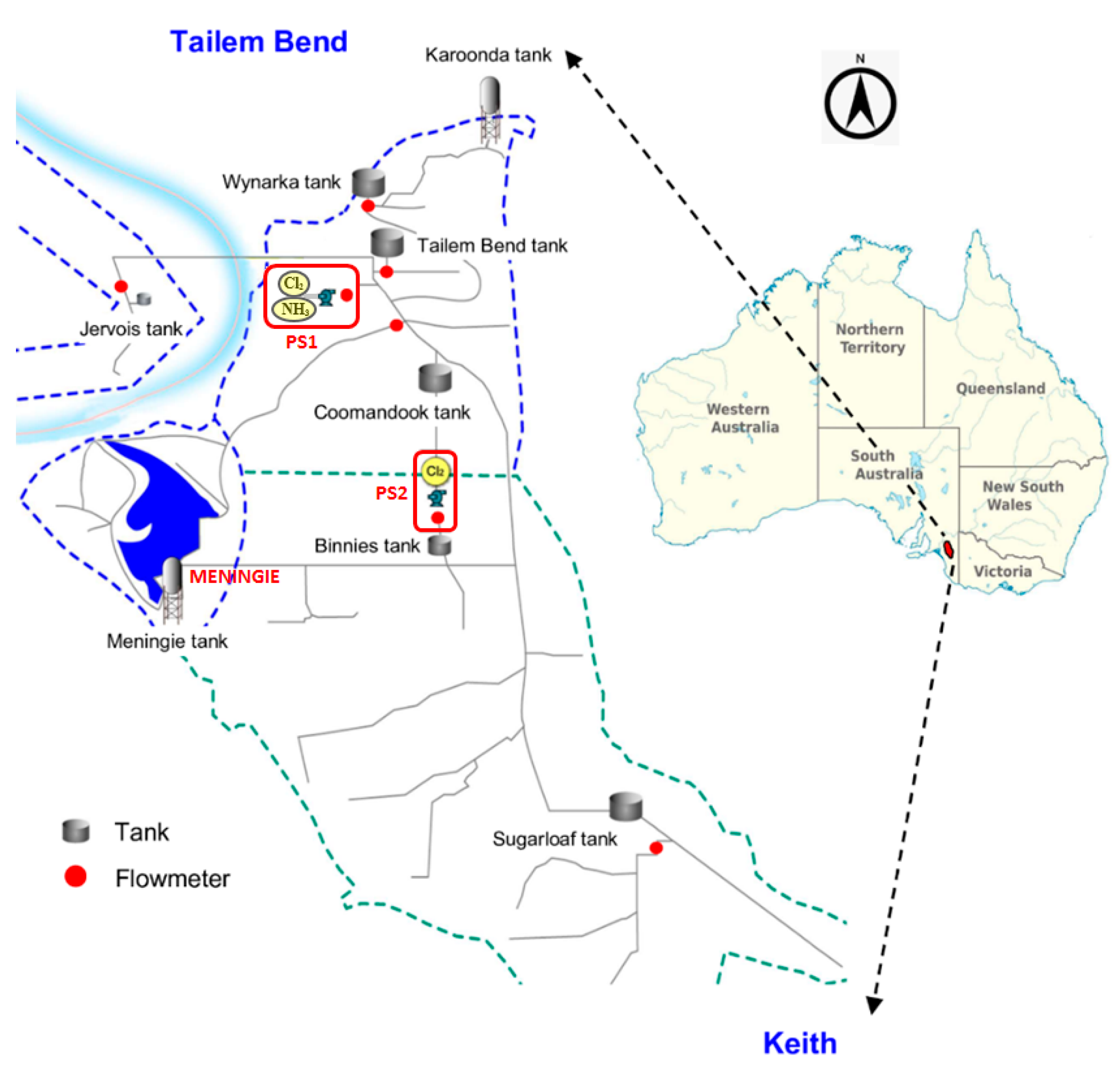
The Tailem Bend-Keith (TBK) drinking water distribution system is one of the largest WDS located in the Tailem Bend township in South Australia. The TBK system extends from the Tailem Bend to Keith communities, consisting of about 130 km long pipeline which feeds about 800 km of branch mains [14,29]. It serves a large area of about 6500 square km, supplying drinking water to customers in Meningie, Karoonda, Keith, and other smaller townships (Figure 1). The water treatment plant (WTP) is located at Tailem Bend and the source water is drawn from the River Murray. Prior to the delivery of treated water to the TBK distribution system, the raw water goes through several stages of treatment using the conventional treatment method (coagulation → flocculation → sedimentation → filtration) followed by disinfection using UV irradiation and chloramination [29]. A schematic of the TBK system with a location map is presented in Figure 1. Initially, ammonia and chlorine are added at pump station 1 (PS1), while at pump station 2 (PS2), chlorine is added to boost the monochloramine residual. Hydraulic and water quality data at strategic locations of the TBK distribution system are monitored using a supervisory control and data acquisition (SCADA) system. It monitors the various hydraulic states of the network including tank levels, pump status, valve status, pressure, and flows. The SCADA system and the subsequent algorithm also monitor a wide range of water quality parameters including the pH, turbidity, chlorine to ammonia ratio, monochloramine, and water age. Additionally, grab samples are routinely collected from several locations of the WDS and analysed for chemical and biological parameters including dissolved organic carbon (DOC), nitrite, nitrate, E. coli, and heterotrophic plate count (HPC). However, at Meningie, the SCADA monitoring system is not available. Water quality at this location is regularly monitored using the grab sampling method. To obtain 30-min resolution water quality data, a spectrophotometer was installed at Meningie. It monitored several water quality parameters including DOC, combined nitrate and nitrite as N (), and turbidity. Additionally, the raw spectral fingerprint was analysed to obtain monochloramine information using the method developed by Hossain et al. [29]. The monochloramine data from PS2 and Meningie were used to calibrate the water quality model for a period of four weeks from early February to March 2021.
2.2. Hydraulic and Water Quality Modelling Tool
The hydraulic and water quality modelling was completed using the EPANET network modelling tool. It is public domain software developed by the U.S. Environmental Protection Agency (USEPA) which can be used to perform either steady-state or an extended period simulation. In EPANET, the whole network system is represented by several interconnected nodes and links. Various other components such as tanks, pumps, and valves, including the pressure sustaining valve (PSV), pressure reducing valve (PRV), and pressure breaker valve (PBV), are used to accurately define a distribution system. The hydraulic solver in EPANET computes nodal head and link flows by simultaneously solving the mass conservation equation in each node and the energy equation in each link [9,30]. The mass conservation and energy equation is given in Equations (1) and (2).
where, is the flow in the link between nodes i and j, and are hydraulic heads at these nodes and is the head loss between them, is the demand at node i, r is a head loss coefficient, n is a flow exponent, and m is a minor loss coefficient.
The head loss coefficient r, of the pipe, is calculated using either the Hazen–Williams, Darcy–Weisbach, or Chezy–Manning formula. Under the most typical condition in a WDS, the Hazen–Williams formula can be used to adequately model head-loss, while the Darcy–Weisbach formula is used to model pressurised flow under a range of hydraulic conditions [9]. In contrast, the Chezy–Manning formula is generally used to model head loss in open channel flow. Pumps are modelled using a curve representing the head vs. flow relationship. For each node, water demand is represented by assuming a baseline demand, and the temporal variability of the baseline demand is modelled using a multiplication factor for each time step [9]. Hydraulic behaviour is accurately simulated by adequately defining control rules in the model for various hydraulic components. In the network, the conservation of mass and energy equations are solved using the global gradient algorithm (GGA) through an iterative process until the convergence criterion is met [31].
The water quality module in EPANET tracks the fate of discrete parcels using the Lagrangian time-based approach as they move through pipes and are mixed together at junctions. Water in a pipe is considered to be a series of non-overlapping segments moving upstream to downstream. The substances in these segments are subjected to reaction, hence, they can grow or decay over time. At each water quality time step, these segment’s positions are updated and new node concentrations are calculated by considering the cumulative amount of mass and flow volume entering each node. The contribution from any external source can also be specified at each node. Four types of water quality sources are available in the EPANET water quality module (i) concentration source, (ii) mass booster source, (iii) set point booster source, and (iv) flow paced booster source [9]. A concentration source fixes the concentration of any external inflow entering a node, a mass booster source adds a fixed mass flow to a node, a set point booster source fixes the concentration of flow leaving a node, and a flow paced booster adds a fixed concentration to a node resulting from the mixing of all inflows. A variable source quality can be modelled by assigning a time pattern.
At service reservoirs, water quality concentrations are updated based on the type of mixing model used for the tanks. The available mixing models are (i) complete mixing, (ii) two-compartment mixing, (iii) the first-in-first-out (FIFO) plug flow model, and (iv) the last-in-first-out (LIFO) plug flow model [9]. The complete mixing model assumes that the water that enters the tank during the filling cycle is instantaneously and completely mixed with the water already residing in the tank. In the two-compartment mixing model, the available storage volume is divided into two compartments, both of which are assumed to be completely mixed. Water parcels enter and exit from the first compartment which, if full, sends overflow to the second compartment which is completely mixed with the water already residing in the second compartment. When water leaves the first compartment, it receives an equivalent inflow from the second compartment. The FIFO plug flow model assumes no mixing of water in the tank during its residence time. Water parcels move through the tank in a segregated fashion where the first parcel to enter is also the first to leave. In the LIFO plug flow model, water parcels entering the tank are assumed to be stacked up one on top of another. There is no mixing between parcels of water as water parcels are assumed to enter and leave the tank on the bottom.
While the dissolved substance is moving through a pipe, water quality reactions are assumed to occur both within the bulk flow and on the materials residing at the pipe surface, including corrosion products and biofilms. The rate of bulk reaction is defined as a power function of concentration as shown in Equation (3).
where, is the bulk reaction rate constant, C is the concentration of the substance being modelled, and n is the reaction order. A first-order reaction is often used to describe the bulk reaction.
Similarly, the water quality reaction occurring at or near the pipe surface is assumed to be a power function of concentration which is given in Equation (4).
where, is the surface area available for reaction per unit volume of water, is a wall reaction rate coefficient, C is the concentration of dissolved substance, and n is the reaction order. This formula suggests that a smaller diameter pipe will be subjected to more reaction as compared to a larger diameter pipe. The rate of wall reaction depends on several factors including the pipe material, pipe age, flow regime, hydraulic conditions, temperature, and water chemistry, hence it should be considered as a calibration parameter.
2.3. Optimisation Tool
PEST (Parameter ESTimation), a non-linear model-independent parameter optimisation tool developed by Watermark Numerical Computing was used to optimise the model parameters. This software can be easily incorporated into several applications in Windows and Linux environments. Because of its model independence, it is increasingly used to calibrate surface water and groundwater models [14,19]. To initiate the calibration in both serial and parallel processing environments, a number of files need to be prepared that contain the settings information of control variables, initial values of parameters and their upper and lower boundaries, information on how to read the result from the simulation output file, and observed data and their corresponding weights and calibration runtime settings. Further details of the calibration setup files can be found in [14,19,32]. Moreover, an objective function is defined which is to be minimised through the calibration process. The default objective function is given by:
where, is the calibration objective function, n is the number of data points, is the assigned weight to the ith measurement, and and are the observed and model-simulated values, respectively. The theoretical minimum value of is positive and zero, meaning a perfect fit. However, it is unlikely to reach a zero value in environmental, hydraulic, and water quality models, instead, a minimum value is sought.
During calibration, the optimisation algorithm takes control of the model and performs hundreds to thousands of iterations to reach the minimum objective function. Four criteria were used to decide the minimum objective function: (i) the convergence of optimisable parameters to their optimal values; (ii) the insignificant reduction in the objective function over successive iterations; (iii) the insignificant change of parameter values over successive iterations; and (iv) the exceedance of the defined maximum number of iterations [32]. Once any of these criteria are fulfilled, the algorithm assumes that the minimum objective function is found, returns the optimum parameter set, and terminates the calibration process.
Optimisation Algorithm
Currently, many algorithms are available for numerical optimisation. These are broadly classified as local and global optimisation. Local optimisation searches parameter values within the parameter’s space that correspond to the local minimum value of the objective function [14,32]. The Gauss–Levenberg–Marquardt algorithm (GLMA), which is a gradient-based method, is an example of local optimisation. In contrast, global optimisation searches for an optimum set of parameters by evaluating many local minimum values of the objective function and retaining the lowest one [32]. Most evolutionary algorithms, including the covariance matrix adaptation evolution strategy (CMAES), particle swarm optimisation (PSO), and the shuffled complex evolution (SCE), are examples of global optimisation. This study used the CMAES algorithm to optimise the model parameters.
The CMAES algorithm is a derivative-free method that has been proven to be successful in minimising non-linear, non-convex, multi-modal, ill-conditioned, or noisy objective functions [21,33]. CMAES minimises the objective function by performing many iterative loops where at each iteration, candidate solutions are generated from the parameter space considering a multivariate Gaussian distribution. Three statistical terms, N(m, , C) are used to represent the multivariate normal distribution, where m is the mean vector, σ is the step-size, and C is a symmetric positive definite matrix, known as the covariance matrix [20,21]. The terms m and σ represent the centre and spread of the distribution, while C is related to the shape of the distribution [14,34]. During each iteration, all candidate solutions are evaluated based on objective function values and sorted accordingly. Prior to the next iteration, the mean of the Gaussian distribution is updated such that the probability of the previously successful candidate solution is maximised while the covariance matrix is updated to maximise the likelihood of previously successful search steps. In the next iteration, the CMAES algorithm adaptively increases or decreases the search space based on the result of the previous iteration [21]. The number of a candidate solution, also referred to as population size, needs to be defined in the CMAES setup. The default population size is given by 4 + 3 ln(n), where n is the number of parameters to optimise. However, in the case of a non-linear, multi-modal, or noisy objective function, the population size should be increased [21,34]. It should be noted that increasing the population size can significantly increase the solution space and the convergence time. The value of σ which represents the initial step size should be defined such that it can be reasonably applied to all variables [14,33].
2.4. Support Vector Regression (SVR)
Support vector machines (SVMs) are supervised machine learning algorithms that can be used for classification and regression problems [35,36,37]. In the classification problem, two different classes of data are separated by using an optimum hyperplane that gives maximum margin around the hyperplane. Hence, the data points falling on either side of the hyperplane can be attributed to different classes. For the regression problem, an epsilon (ε) range is assumed from both sides of the hyperplane where the regression error by the points within the ε distance is ignored [37,38]. Therefore, the best fit line in SVR is the hyperplane that has the maximum number of points. If the data points are linearly inseparable in a classification problem, a kernel function is used to map the data in a high-dimensional or feature space where linear separation exists [36,38]. A kernel function is defined as a linear dot product in the feature space. Different kernel functions give different mapping capabilities. Except for ε, two other parameters of the SVR algorithm are C and Υ, where C represents the penalty of misclassifying a data point and Υ controls the spread of the data while transforming to a feature space. A relatively low value of Υ encounters a broader decision region while a high Υ creates islands of decision boundaries around data points. These parameters are fine-tuned to obtain the optimum hyperplane. Among the available kernel functions, the right choice of kernel may improve the SVR modelling performance. The most commonly used kernel functions in the SVR algorithm are given in Equations (6)–(9):
where, is the transpose of , r is a constant term, is the polynomial order, and is an RBF kernel parameter.
2.5. Sampling Strategy and Laboratory Procedures
Typically, the bulk decay coefficient is determined using the disinfected water collected from the point of entry to the WDS. Chloraminated grab samples were collected from the TB-WTP at different periods. These samples were stored in amber bottles and kept in a dark place at a temperature of 24 ± 1 °C, which was assumed to be the average temperature of the WDS during the study period. Otherwise, the Arrhenius equation can be used to adjust the temperature effect. As the bulk decay coefficient can be different for different samples, five individual experiments were conducted to decide the typical bulk decay coefficient during the study period. The N,N-diethyl-p-phenylenediamine (DPD)-ferrous ammonium sulfate (FAS) titrimetric procedure (APHA 4500-CI-F) was used to determine the free chlorine, monochloramine, and dichloramine concentrations [39]. Temperature and pH were determined using a portable pH meter (pH320, WTW, Weilheim, Germany). The decay of these samples was observed for a period of four weeks.
2.6. Model Setup
In the water quality model setup in EPANET, the quality time step was selected as 5 min. The bulk and wall decay coefficients were assigned to be first-order reactions. For automatic calibration, initial values of parameters and the ranges within which they vary need to be provided to the optimisation algorithm. The bulk decay coefficient established through the lab experiment was used as an initial value with a little tolerance above and below for the range, while for the wall decay coefficient, the initial values and the ranges were obtained from the literature. In a distribution system, the water stays in service reservoirs most of the time rather than in pipes. Wall reactions can also occur in tanks. However, unlike in a pipe wall, a constant wall surface is not possible in a tank because of its filling and emptying. Hence, on top of bulk decay, an additional loss was assumed in tanks for wall reaction. For all tanks, a first-order reaction was assumed and the final value was obtained through calibration. The re-chlorination point was modelled using a “setpoint booster” in EPANET. The optimisation process can take several hours to days to complete depending on the problem size. Using the CMAES global search algorithm, the optimisation was performed in a Linux-based high-performance computing (HPC) environment. The settings of the CMAES algorithm parameters control the convergence time which was left to default values. Parallel processing was employed to reduce the optimisation time. R programming language [40] was incorporated with EPANET and the optimisation tool. They act sequentially to update the model input file during each model run throughout the optimisation process.
In preparing the data analytics model, the various water quality parameters at the point of chloramine application were included. Water age at the points where monochloramine concentrations were modelled were obtained from the EPANET simulation and included in the data analytics model. Data were normalized to the +1 and −1 range to bring their values to a common scale so that model training was not very sensitive to variables with high values. The Unscrumbler X (CAMO software, Oslo, Norway) was used to create the SVR model. The performances of the SVR model were investigated under different kernel functions as shown in Equations (6)–(9).
3. Results and Discussion
3.1. Typical Water Quality at the Studied Locations
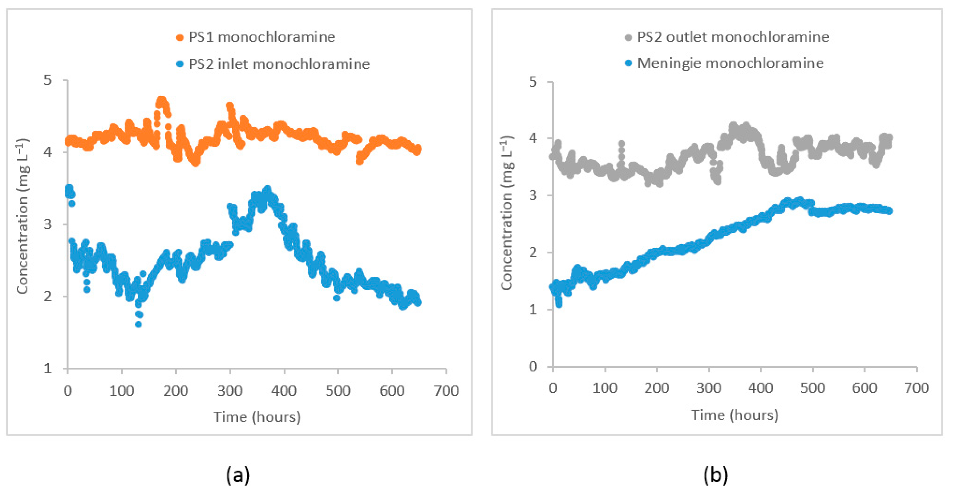
The monochloramine concentrations were simulated at two separate monitoring points in the distribution system (i) at the PS2 inlet and (ii) at the Meningie pump station. During the study period, the monochloramine concentration at PS1 where chloramination is applied was 4.2 ± 0.1 . When these monochloramine residuals reached the PS2 inlet, their concentration was reduced to 2.5 ± 0.4 because of residual decay through bulk and wall decay processes. At the PS2 outlet, re-chlorination is done to boost the monochloramine concentration to 3.7 ± 0.2 . At Meningie, the residual concentration decreased to 2.3 ± 0.5 . The concentration of dichloramine and free chlorine at these locations was below the reporting limit for field titration (<0.1 ). There was high variability in monochloramine concentration at the PS2 inlet and Meningie compared to its variability at the PS1 and PS2 outlet. A reduction in pH was also observed at Meningie (pH = 8.5 ± 0.3) compared to the PS1 (pH = 9.0 ± 0.1) and PS2 outlet (pH = 9.7 ± 0.1 after adjustment), which could possibly be caused by the products of monochloramine decomposition and/or wall reactions. The turbidity at PS1 was 0.07 ± 0.01 nephelometric turbidity unit (NTU), while DOC and concentrations were 2.0 ± 0.2 and 0.2 ± 0.1 , respectively. As shown in Figure 2, the monochloramine data from these locations suggest that bulk and wall decay processes cause a significant reduction in monochloramine residuals while traveling from Tailem Bend to Meningie.
3.2. Development and Calibration of Hydraulic Model
The details of the hydraulic model development and calibration process for the TBK system can be found in Hossain et al. [14]. In brief, the model was constructed using various information such as the initial states of several hydraulic components, their geometry, and settings. For pipe head loss calculation, the Hazen–Williams formula was used, while the hydraulic time step was set to 30 min. Some missing values and outliers were found in the SCADA data which were replaced by the closest sensible values. Two different demand patterns were considered: residential and commercial. Several parameters including pipe roughness, pump settings, time-based controls for pump operation, and parameters representing variable demand patterns were calibrated. An automatic calibration method using the CMAES global optimisation algorithm was adopted. The calibration process was run in a Linux-based high-performance computing environment (HPC). Several codes were composed to run the whole calibration process in order.
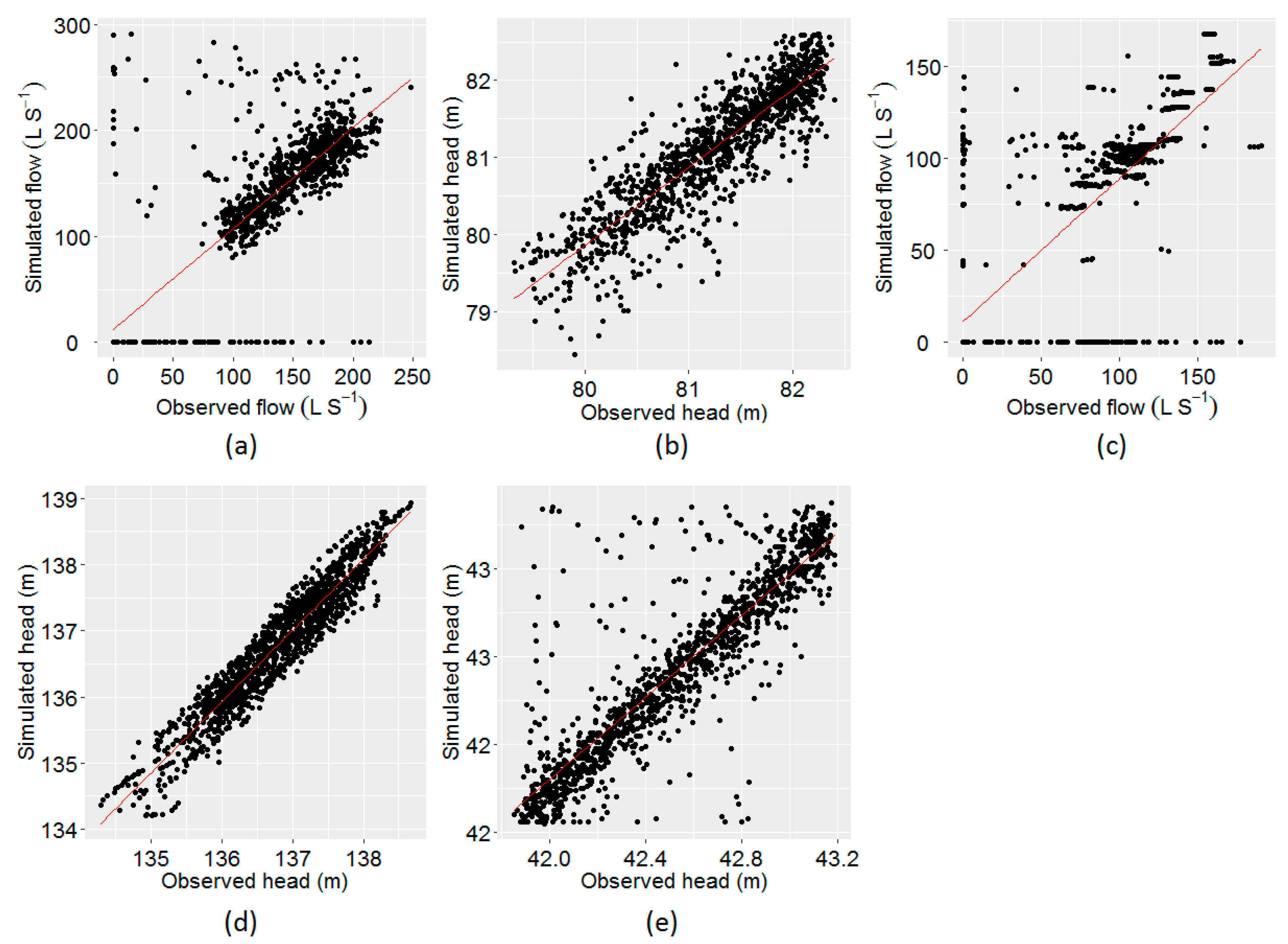
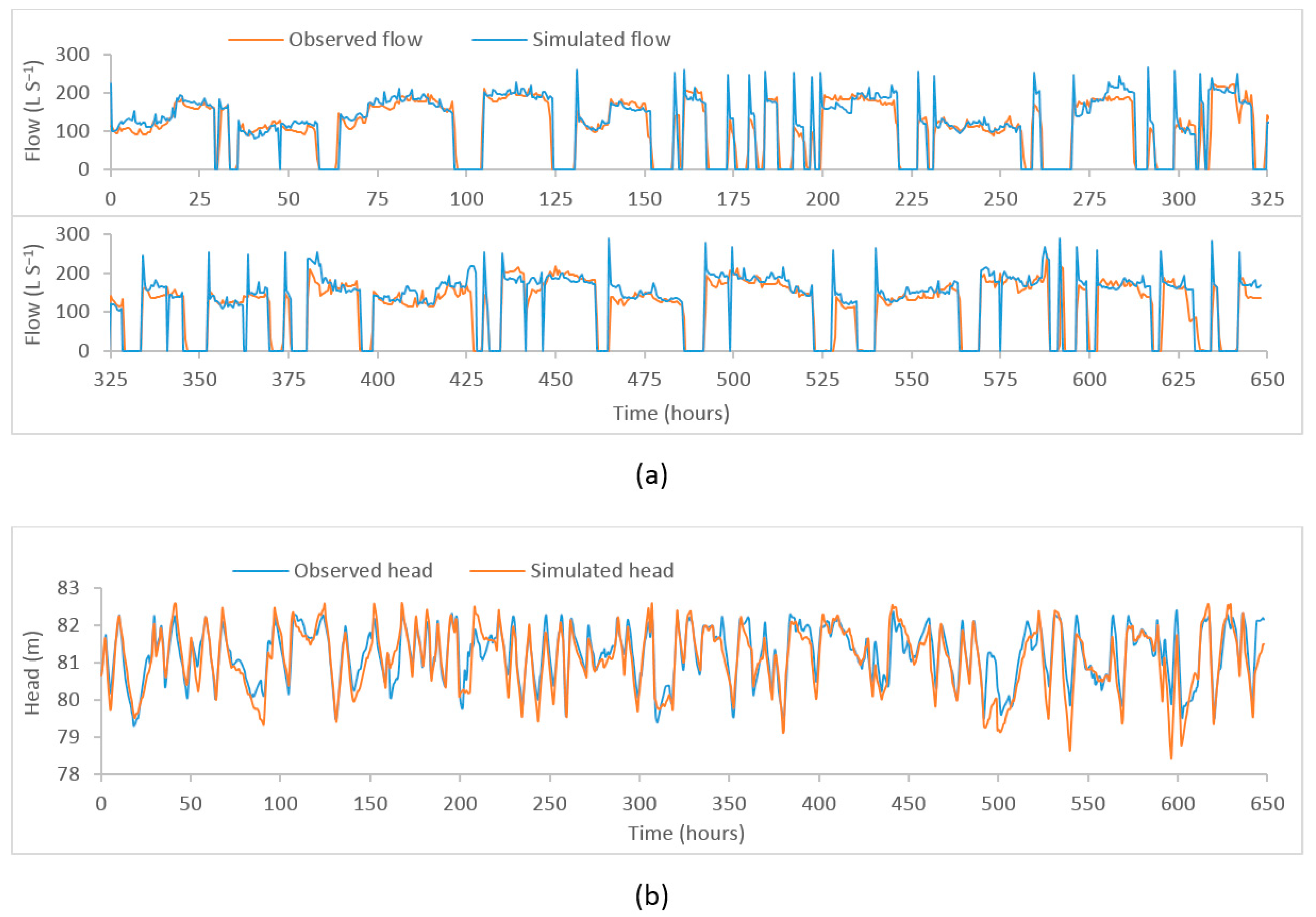
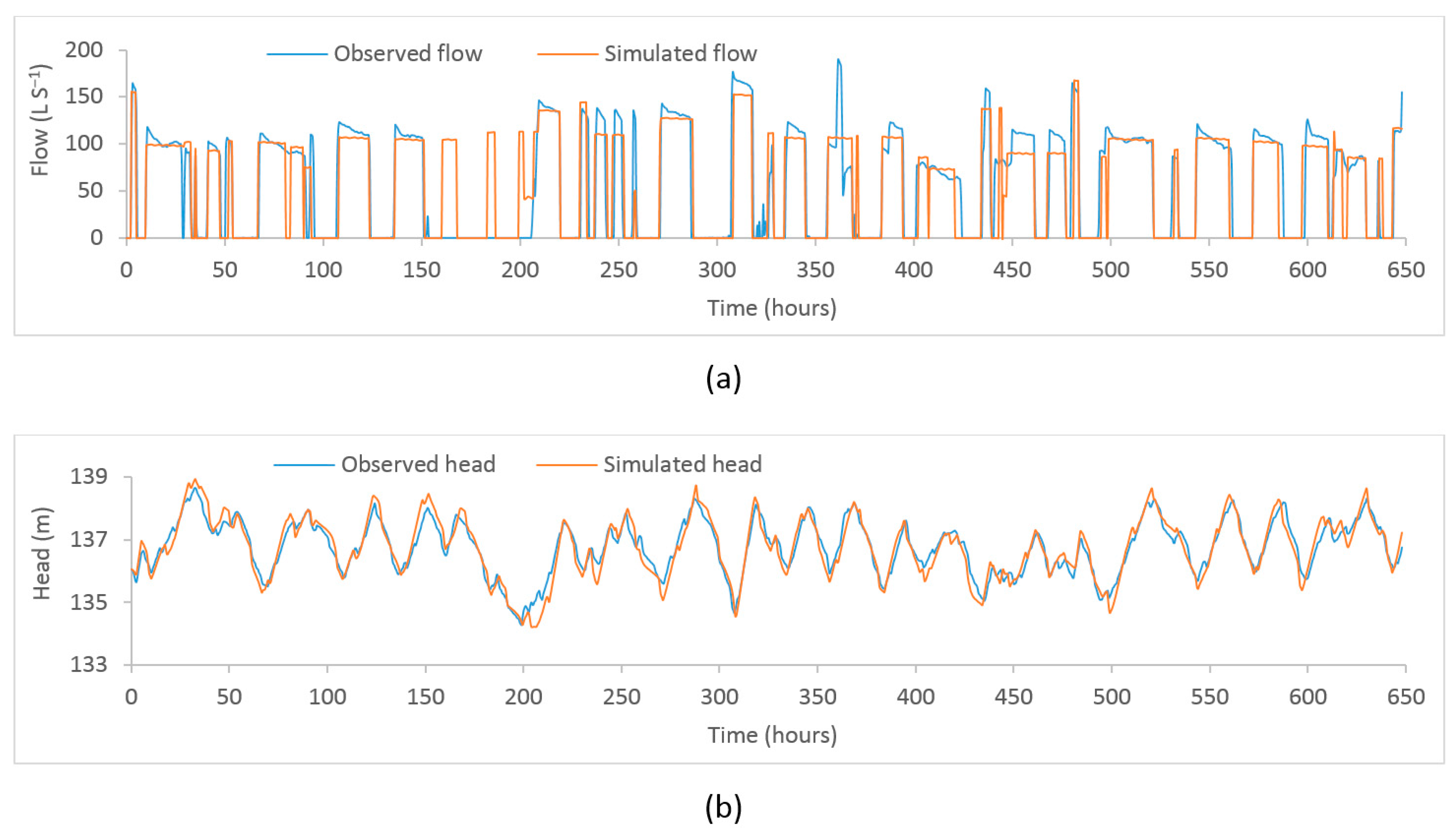
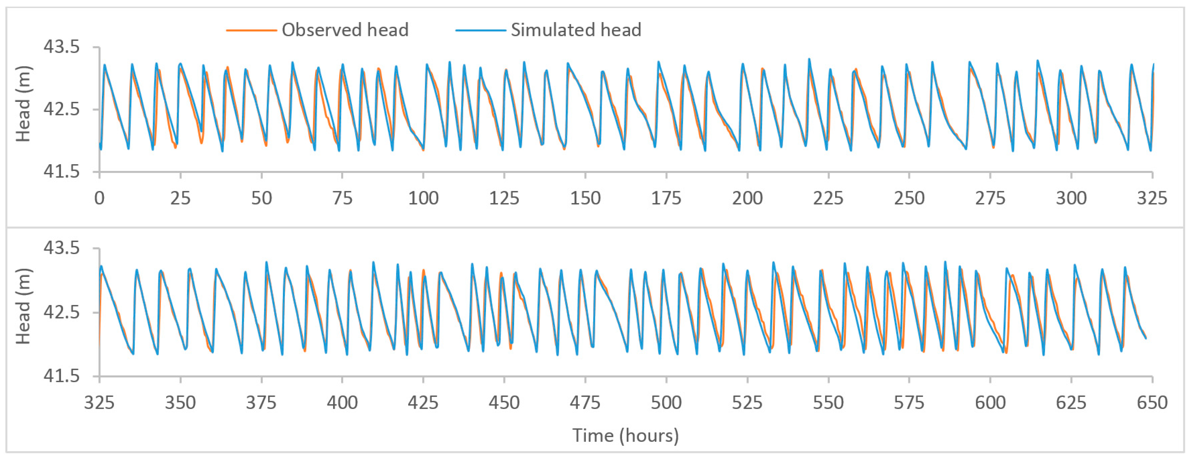
Through the calibration process, the objective function was minimised to obtain the maximum fit between the observed and the simulated time series. The plot of observed vs. model simulated tank heads and flows corresponding to the best objective function at five different locations (i) flow at PS1, (ii) head at Coomandook tank, (iii) flow at PS2, (iv) head at Binnies tank, and (v) head at Meningie tank are presented in Figure 3. The plot of the whole time series at these locations is given in Figure A1, Figure A2 and Figure A3 in Appendix A. The correlation between the observed and the simulated heads at Coomandook, Binnies, and Meningie tanks were 0.88, 0.95, and 0.88 while the correlation between the observed and the simulated flows at PS1 and PS2 were 0.85 and 0.80. The mean of the observed heads at Coomandook, Binnies, and Meningie were 81.23 m, 136.77 m, and 42.53 m while the same obtained through model simulation were 81.1 m, 136.76 m, and 42.54 m, respectively. In contrast, the mean of the observed and model-simulated flows at PS1 were 113.84 and 120.68 while those at PS2 were 57.19 and 55.92 , respectively. The percentage difference between observed and simulated flows at PS1 and PS2 were 5.83% and 2.25%, respectively. Therefore, the developed hydraulic model was considered adequately calibrated to reproduce the observed data.
3.3. Bulk Decay Study
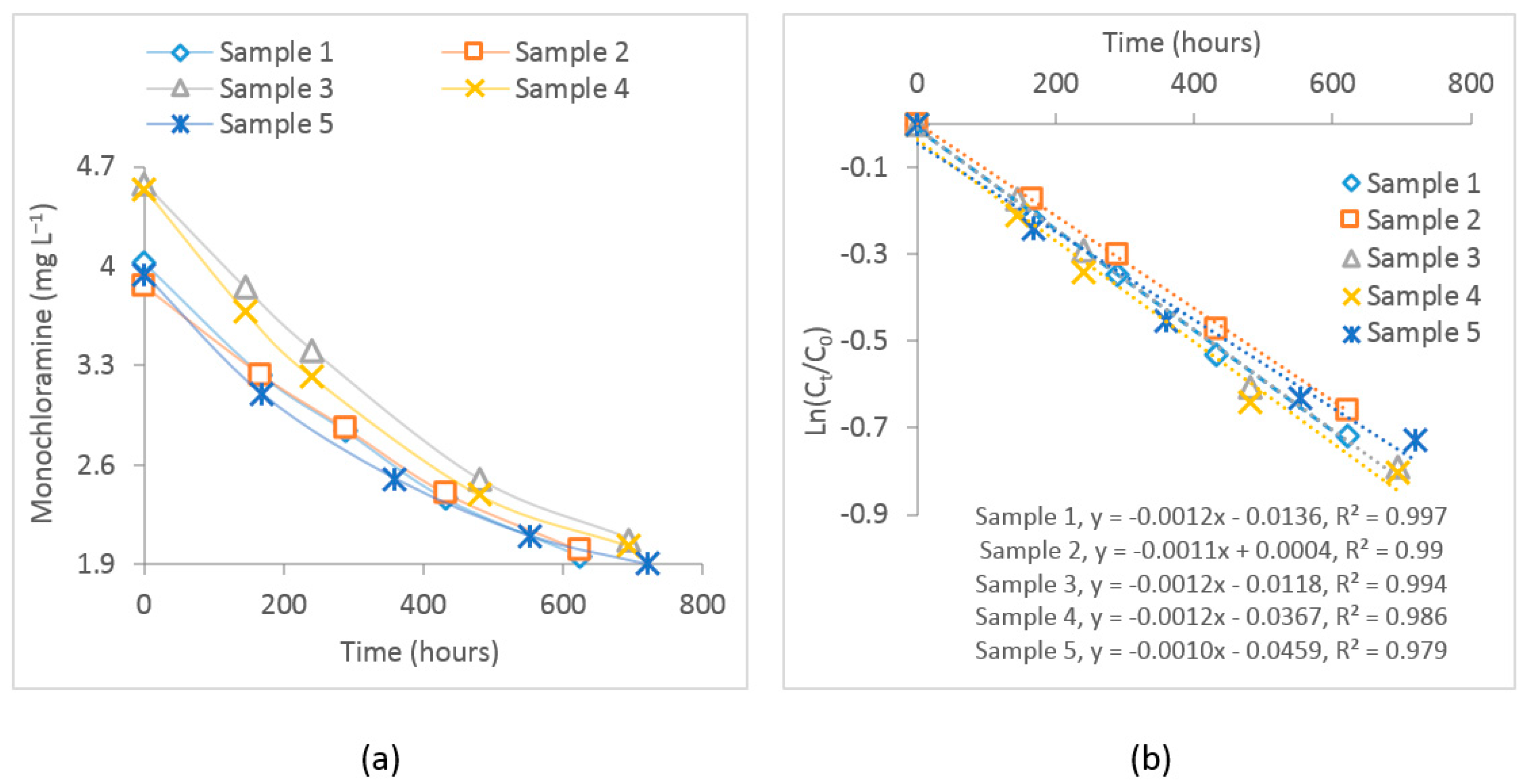
The measured free chlorine and dichloramine concentrations in the five samples during the four-week observation period were below the reporting limit (<). For all samples, the bulk decay coefficients of monochloramine were determined by fitting a first-order decay curve. The average value of these coefficients was considered as the bulk decay coefficient in calibrating the water quality model. Figure 4 shows the observed monochloramine decay and the subsequent first-order curve fitting where the slope of the line represents the bulk decay coefficient. The estimated value of the average bulk decay coefficient for these samples was −0.0012 . The bulk decay coefficient can be changed due to changes in pH and temperature. Therefore, considering it as the starting point, this value was also calibrated, representing the average bulk decay coefficient during the study period.
3.4. Water Quality Model Calibration and Validation
Observed data from the selected locations were used to calibrate the EPANET water quality model. The parameters representing bulk and wall decays, tank reaction rates, and initial monochloramine residual concentrations were included in the calibration process. The initial monochloramine concentration can be gradually reduced as the distance from the source increases because of residual decay. Therefore, the whole distribution system is arbitrarily divided into several zones and for each zone, individual initial concentrations were assigned which were also calibrated. The calibrated value of the first-order bulk decay coefficient for the flow path from PS1 to the PS2 inlet (path 1) was −0.0012 while for the PS2 outlet to Meningie (path 2) was −0.001 . For path 2, the calibrated bulk decay coefficient was relatively low as compared to that for path 1. This is because the monochloramine bulk decay rate decreased with the increased water age. Similarly, this variation can also be attributed to varying pH and temperature throughout the system. In contrast, the calibrated first-order wall decay coefficient for path 1 was −0.029 m while path 2 was −0.006 m . For path 1, most pipe diameters varied from 610 mm to 758 mm while for path 2, most pipe diameters ranged between 102 mm to 363 mm. The calibrated wall decay coefficients represent average values for the whole path. The fit between the observed and the simulated monochloramine residual concentration as obtained through the calibrated model was measured by the Root Mean Square Error (RMSE) and coefficient of determination (R2). Figure 5 shows the observed and the simulated monochloramine concentration plots at the PS2 inlet and Meningie and corresponding correlation plots for these locations. At the PS2 inlet, the calibration performance in terms of RMSE and R2 were 0.007 and 0.66, respectively, while at Meningie, the performances were 0.009 and 0.94. The model’s performance at the PS2 inlet was relatively poor as compared to that at Meningie, which can be attributed to many factors including pH and temperature changes and the quality of the observed data used in model calibration.
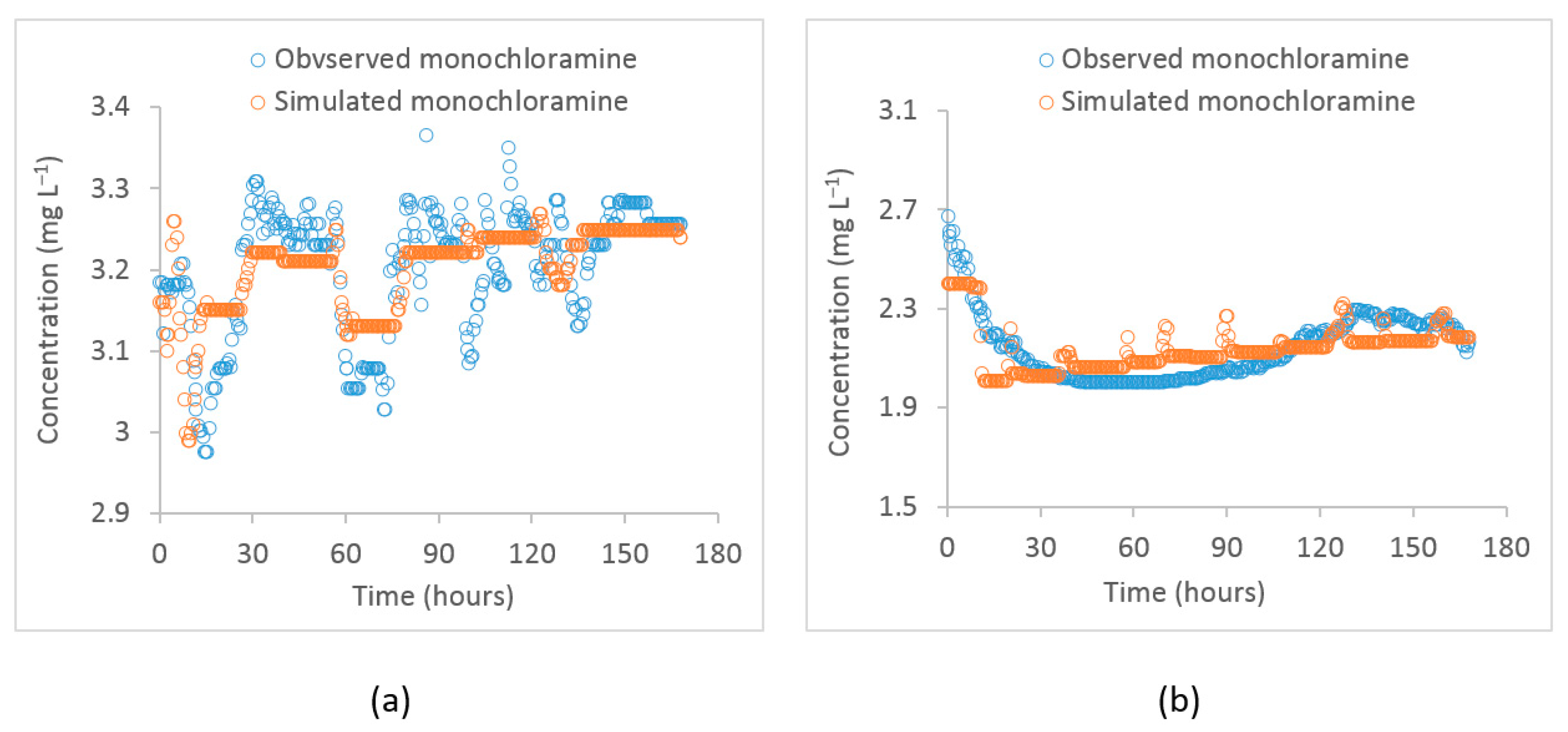
For the water quality model validation, another hydraulic model was constructed in EPANET using a different data period. The hydraulic model was adequately calibrated for one week. Then, the water quality model was run with the previously obtained calibrated water quality parameters. The time-series plots of the observed vs. the simulated monochloramine concentrations at the PS2 inlet and Meningie during the validation period are shown in Figure 6. The correlation between the observed and model-simulated values at the PS2 inlet were 0.64 and 0.74 at Meningie. During the validation period, the mean of the observed monochloramine concentrations at PS2 inlet and Meningie were 3.2 ± 0.1 and 2.1 ± 0.1 , respectively, while the same simulated values for these locations were 3.2 ± 0.1 and 2.1 ± 0.1 , respectively. These statistics indicate that the calibrated water quality model can reasonably reproduce the observed monochloramine concentrations during the validation period.
3.5. Machine Learning Model
To improve the monochloramine prediction at these locations, machine learning models were developed using the SVR algorithm. The SVR model used observed water quality data from the source point or point of chloramine application including monochloramine concentration, flow, pH, turbidity, DOC, , and water age at the points of interest as predictor variables, while the observed monochloramine concentration at the points of interest were used as response variables. An epsilon value of 0.01 and 10-fold cross-validation were employed. A grid search method was used to find the optimum SVR function parameters. Modelling performances under different kernel functions such as linear, polynomial, RBF, and sigmoid were investigated (Table 1), and the RBF was found to be the most accurate kernel to map the data. Figure 7 shows the plot of observed vs. model predicted time-series at the PS2 inlet and Meningie and corresponding correlation plots using the RBF kernel. At the PS2 inlet, RMSE and R2 in model training were 0.03 and 0.99 while in cross-validation, they were 0.11 and 0.92, respectively. Similarly, at Meningie, RMSE and R2 during SVR model training were 0.03 and 0.99, while the same during cross-validation were 0.05 and 0.99. These statistics suggest that the developed SVR model can adequately predict the monochloramine concentrations at the studied locations.
3.6. Discussion and Future Work
This study suggests that both the water quality network model and data analytics model can adequately predict the observed monochloramine concentrations at the studied locations. However, the data analytics model shows a relatively higher performance as compared to the water quality network model. The water quality network model’s performance can be improved by accurately defining the initial water quality conditions throughout the network. It should be noted that the water quality network model is a more practical option for most WDS as it requires only a few water quality data, such as the decay rate and initial concentrations, to simulate the monochloramine profile throughout the network. In contrast, the data analytics model requires several water quality data, hence, it becomes impractical for WDS that do not employ real-time monitoring for a range of water quality parameters.
Monochloramine decay is a complex process that depends on several chemical and microbiological factors. The bulk decay rate determined in the laboratory mainly consists of monochloramine auto-decomposition, decay due to NOM, and microbiological reactions. It is evident that for the same initial monochloramine concentration, the individual decay component can vary with the changed water quality including pH, temperature, and the concentration of NOM and microbiological cells, hence, the overall bulk decay rate also varies. Moreover, the variability of flow rate and the mixing condition in the tank can alter the water chemistry and can affect the overall monochloramine decay rate. Therefore, the bulk decay parameter was also calibrated by assuming a little tolerance above and below the value obtained from the lab experiment. The calibrated parameters are expected to minimise the temperature effect on the bulk and wall decay rates, and they represent average values for the whole path.
Literature suggests that monochloramine is more stable at a higher pH. During the course of the bulk decay experiment, pH was found to decrease, which could be due to monochloramine decomposition reactions. In the case of real WDS, the products of bulk and wall reactions may also contribute to reducing the pH of water which can significantly accelerate the monochloramine decay rate. However, at the studied WDS, pH was re-adjusted at an intermediate point at PS2 to maximise the monochloramine stability. Hence, the monochloramine decay rate was assumed to be approximately stable. For WDS where a significant reduction in pH occurs between the source point and the point of interest, one might encounter a poor calibration performance because of the variable decay rate. In such a case, using a relatively shorter period of data for model calibration may improve the calibration performance.
Pipe materials can significantly affect the chloramine decay, hence, for a specific WDS, the wall decay coefficient can vary in different parts of the distribution system. In a review, Hossain et al. [8] suggested that cement pipes can affect chloramine decay as the principal ingredients of cement are aluminosilicates which can be reactive to chloramine. They can also leach lime over time which may change the pH of the water and affect the chloramine stability. Similarly, pipes made of polyvinyl chloride (PVC) can leach organic compounds, including plasticisers, which affect chloramine decay. Westbrook and Digiano [6] reported the chloraminated wall decay coefficient of 0.67 m d−1 in cast iron (CI) pipe and 0.026 m d−1 in ductile iron (DI) pipe. Similarly, Liu [41] determined the chloraminated wall decay coefficient of 0.046 m d−1 in many areas of the distribution where CI pipes dominate, whereas it was reduced to 0.0160 m d−1 where the pipe material was mostly made of PVC. In our study, the estimated wall decay coefficient varied from 0.15 m d−1 to 0.69 m d−1 dependent on pipe category, and the dominant pipe category of the distribution system was asbestos cement (AC). Other pipe categories such as PVC and DI are also found in some areas of the distribution system. Hence, the quantified wall decay coefficient through parameter optimisation is consistent with the previous studies.
Wall decay is very site-specific and depends on several factors including pipe diameter, pipe material, and age [8,42]. The estimated wall decay coefficient in the current study reflects the decay associated with the dominant pipe category. For better accuracy, the flow path should be divided into several zones and for each zone, an individual wall decay coefficient should be assigned to minimise the error caused by different pipe materials or age. Future studies should consider this aspect.
In a distribution system, a significant amount of monochloramine decay happens in service reservoirs [43]. The mixing condition largely characterises the monochloramine decay dynamics in the reservoir. This study assumes complete and instantaneous mixing which can be changed depending on several factors including the flow rate, seasonal variation of water usage, and customer demand. Further research is necessary to better understand the mixing pattern and the subsequent decay characteristics in the reservoir. Possibly, other available mixing models such as two-compartment mixing, FIFO, and LIFO plug flow mixing can be explored. In addition, the current studies used the CMAES global search algorithm to calibrate the water quality network model parameters; calibration performance under other global optimisations should be an area to explore further.
A data-driven model can be used without the development of a hydraulic model for a WDS [22,25]. However, the current study developed a data analytics model using some variables that were obtained through hydraulic model simulation. Using significant parameters helps reduce the model size by removing redundant information and decreasing the noise introduced in the model [22]. In a chlorinated system, Gibbs et al. [22] identified the significant parameters for an ANN model were upstream chlorine concentration, flow, and temperature. Similarly, using a data-driven approach, Peters et al. [25] found that reservoir total chlorine and temperature can capture 90% of the variability in the downstream total chlorine, while the turbidity, pH, and chlorine to ammonia ratio have a relatively smaller effect. The significant parameters found in this study are upstream monochloramine concentrations, pH, DOC, and water age, while flow, turbidity, and have relatively less effect on the downstream monochloramine concentration. At the PS2 inlet, these significant parameters upstream can capture 93% of the variability in the downstream monochloramine concentration during model training and 88% variability during cross-validation.
While the current study used the SVR method to develop the data analytics model, the modelling performance can be different under different ML algorithms. Further studies may investigate the data analytics modelling performance using different ML algorithms. The performance can also be improved by including more water quality variables. Due to data unavailability, the current study does not include the temperature variable in the data analytics model. As temperature is one of the crucial factors controlling monochloramine decay, incorporating it into the model may better explain the relationship between the variables and improve the model’s predictability. In addition, microbiological activity can significantly affect the monochloramine decay process. Hence, further research is necessary to identify and incorporate these important microbiological parameters.
The calibrated water quality network model can be better used to predict the monochloramine concentration for a different period if the water quality is relatively stable and similar to the calibration period. If there is a significant change in water quality, its chemistry may change which can alter the bulk and wall decay kinetics. In such a case, the model needs to be re-calibrated using the observed data to obtain a better prediction. The procedure/method adopted in this study has shown good chloramine predictability, hence, it can be applied to a different distribution system. The developed model is a site-specific model which is valid only for the case-studied system. For a different distribution system, the hydraulic and water quality characteristics may be different, hence the need to re-develop and/or re-calibrate the hydraulic, water quality, and data analytics model for that system.
4. Conclusions
Management of disinfectant residuals in a distribution system is important to ensure water is microbiologically safe to consume. From the entry point where disinfectant is applied to the customer taps, the residual monochloramine gradually decays during its passage through the network. From a water quality modelling viewpoint, monochloramine decay can be modelled using bulk and wall decay kinetics. The bulk decay coefficient for a specific distribution system can be quantified in the laboratory through controlled laboratory experiments, while wall decay is difficult to quantify as it depends on several factors including pipe materials, pipe age, and the density of biofilms and corrosion products. In this paper, we have quantified the wall decay coefficient using the parameter optimisation technique. For this purpose, a hydraulic model of the studied distribution system was constructed and adequately calibrated to reproduce the observed data at the selected locations. Then, the water quality model was formulated by assigning bulk and wall decays. The bulk decay, as obtained through lab experiments, was assigned to the model while the initial value of the wall decay coefficient and range were obtained from the literature. The CMAES, which is a global search algorithm, was used to optimise the water quality model parameters. The whole calibration process was run in a Linux-based HPC environment using parallel processing. Several types of software were incorporated together to run the whole calibration process in order.
Using the calibrated wall decay parameters, the water quality model-simulated monochloramine residual concentrations were compared with the observed data at two different locations in the Tailem Bend drinking water distribution system located in South Australia. For the first location (PS1), the goodness-of-fit between the observed and simulated monochloramine residual concentration was , while for the second location, the fit was . The calibrated water quality network model was validated using a different data period and found to reasonably reproduce the observed data.
To improve the model prediction at these locations, data analytics models were developed using machine learning algorithms. Various hydraulic and water quality data such as flow rate, water age, pH, DOC, and monochloramine concentrations at the source point and the point of interest were used to build the data analytics model. Using the SVR algorithm and a 10-fold cross-validation, the model’s performance was compared under different kernel functions. The RBF was found to be the most appropriate kernel to map the data. The performance at PS2 in the SVR model training was and cross-validation was . In contrast, at Meningie, the SVR performance in both model training and cross-validation was . At both locations, the SVR models reproduced the observed data with a high level of accuracy. The key findings are (i) the estimated wall decay coefficient for the TBK system varies from 0.15 m d−1 to 0.69 m d−1, depending on the pipe diameter, (ii) the significant parameters in the data analytics model are upstream monochloramine concentration, pH, water age and DOC concentrations, (iii) the RBF is the most appropriate kernel function to analyse data using the SVR method, and (vi) the upstream flow, turbidity and concentrations have little effect on downstream monochloramine. Finally, it can be concluded that, at the studied locations, the water quality network model and data analytics model both adequately predict the observed data. However, the data analytics model showed better predictability, and hence, is recommended if various water quality data are available.
Author Contributions
Conceptualisation, S.H., G.A.H., C.W.K.C. and D.C.; Data curation, S.H.; Formal analysis, S.H.; Funding acquisition, G.A.H., C.W.K.C. and D.C.; Investigation, S.H., G.A.H., C.W.K.C. and D.C.; Methodology, S.H., G.A.H., C.W.K.C. and D.C.; Resources, G.A.H., C.W.K.C. and D.C.; Software, S.H.; Supervision, G.A.H., C.W.K.C. and D.C.; Validation, S.H., G.A.H., C.W.K.C. and D.C.; Writing—original draft, S.H.; Writing—review and editing, G.A.H., C.W.K.C. and D.C. All authors have read and agreed to the published version of the manuscript.
Funding
This research received funding from the University of South Australia through the postgraduate scholarship award scheme. Additional funding was received from the South Australian Water Corporation through Water Research Australia (project number 4535-17).
Institutional Review Board Statement
Not applicable.
Informed Consent Statement
Not applicable.
Data Availability Statement
Data will be available on request.
Acknowledgments
This work was supported by the University of South Australia, South Australian Water Corporation, Water Research Australia, TRILITY, and DCM Process Control. The authors acknowledge all parties for their contribution to the project.
Conflicts of Interest
The authors declare no conflict of interest.
Appendix A
Figure A1.
Plot of observed and model–simulated time–series. (a) Flow at PS1 (b) head at Coomandook tank.
Figure A1.
Plot of observed and model–simulated time–series. (a) Flow at PS1 (b) head at Coomandook tank.

Figure A2.
Plot of observed and model–simulated time–series. (a) Flow at PS2 (b) head at Binnies tank.
Figure A2.
Plot of observed and model–simulated time–series. (a) Flow at PS2 (b) head at Binnies tank.

Figure A3.
Plot of observed and model-simulated time-series for the head at Meningie tank.

References
- Kirmeyer, G.; Martel, K.; Thompson, G.; Radder, L.; Klement, W.; Le Chevallier, M.; Baribeau, H.; Flores, A. Optimizing Chloramine Treatment, 2nd ed.; American Water Works Association: Denver, CO, USA, 2004. [Google Scholar]
- Vikesland, P.J.; Ozekin, K.; Valentine, R.L. Monochloramine Decay in Model and Distribution System Waters. Water Res. 2001, 35, 1766–1776. [Google Scholar] [CrossRef]
- Duirk, S.E.; Gombert, B.; Choi, J.; Valentine, R.L. Monochloramine loss in the presence of humic acid. J. Environ. Monit. 2002, 4, 85–89. [Google Scholar] [CrossRef] [PubMed]
- Duirk, S.E.; Gombert, B.; Croué, J.P.; Valentine, R.L. Modeling monochloramine loss in the presence of natural organic matter. Water Res. 2005, 39, 3418–3431. [Google Scholar] [CrossRef]
- Jafvert, C.T.; Valentine, R.L. Reaction scheme for the chlorination of ammoniacal water. Environ. Sci. Technol. 1992, 26, 577–586. [Google Scholar] [CrossRef]
- Westbrook, A.; Digiano, F.A. Rate of chloramine decay at pipe surfaces. J.-Am. Water Work. Assoc. 2009, 101, 59–70. [Google Scholar] [CrossRef]
- Ejigu, M.T. Overview of water quality modeling. Cogent Eng. 2021, 8, 1891711. [Google Scholar] [CrossRef]
- Hossain, S.; Chow, C.W.K.; Cook, D.; Sawade, E.; Hewa, G.A. Review of chloramine decay models in drinking water system. Environ. Sci. Water Res. Technol. 2022, 8, 926–948. [Google Scholar] [CrossRef]
- Rossman, L.A. Epanet 2 Users Manual; US environmental Protection Agency, Water Supply and Water Resources Division, National Risk Management Research Laboratory: Cincinnati, OH, USA, 2000.
- Westbrook, J.A. Determination of Chloramine Decay Rates at Pipe Surfaces and in Bulk Water in a Simulated Distribution System Environment. Master’s Thesis, University of North Carolina, Chapel Hill, NC, USA, 2006. [Google Scholar]
- Speight, V.; Boxall, J. Current Perspectives on Disinfectant Modelling. Procedia Eng. 2015, 119, 434–441. [Google Scholar] [CrossRef] [Green Version]
- Shang, F.; Uber, J.G.; Rossman, L.A. Modeling Reaction and Transport of Multiple Species in Water Distribution Systems. Environ. Sci. Technol. 2008, 42, 808–814. [Google Scholar] [CrossRef]
- Wilczak, A.; Jacangelo, J.G.; Marcinko, J.P.; Odell, L.H.; Kirmeyer, G.J. Occurrence of nitrification in chloraminated distribution systems. J.-Am. Water Work Assoc. 1996, 88, 74–85. [Google Scholar] [CrossRef]
- Hossain, S.; Hewa, G.A.; Chow, C.W.K.; Cook, D. Modelling and Incorporating the Variable Demand Patterns to the Calibration of Water Distribution System Hydraulic Model. Water 2021, 13, 2890. [Google Scholar] [CrossRef]
- Shen, H.; McBean, E. Hydraulic calibration for a small water distribution network. In Water Distribution Systems Analysis 2010; American Society of Civil Engineers: Reston, VA, USA, 2010; pp. 1545–1557. [Google Scholar]
- Doshi, B.; Grayman, W.M.; Guastella, D. Field testing the chlorine wall demand in distribution mains. In Proceedings of the 2003 AWWA Annual Conference, Anaheim, CA, USA, 15–19 June 2003; pp. 1–10. [Google Scholar]
- Monteiro, L.; Figueiredo, D.; Dias, S.; Freitas, R.; Covas, D.; Menaia, J.; Coelho, S.T. Modeling of Chlorine Decay in Drinking Water Supply Systems Using EPANET MSX. Procedia Eng. 2014, 70, 1192–1200. [Google Scholar] [CrossRef] [Green Version]
- Alexander, M.T.; Boccelli, D.L. Field Verification of an Integrated Hydraulic and Multi-Species Water Quality Model. In Proceedings of the 12th Annual Conference on Water Distribution Systems Analysis, Tucson, AZ, USA, 12–15 September 2010; pp. 687–697. [Google Scholar]
- Doherty, J.; Skahill, B.E. An advanced regularization methodology for use in watershed model calibration. J. Hydrol. 2006, 327, 564–577. [Google Scholar] [CrossRef]
- Hansen, N.; Kern, S. Evaluating the CMA Evolution Strategy on Multimodal Test Functions. In Parallel Problem Solving from Nature—PPSN VIII; Springer: Berlin/Heidelberg, Germany, 2004; pp. 282–291. [Google Scholar]
- Hansen, N.; Ostermeier, A. Completely Derandomized Self-Adaptation in Evolution Strategies. Evol. Comput. 2001, 9, 159–195. [Google Scholar] [CrossRef] [PubMed]
- Gibbs, M.S.; Morgan, N.; Maier, H.R.; Dandy, G.C.; Nixon, J.B.; Holmes, M. Investigation into the relationship between chlorine decay and water distribution parameters using data driven methods. Math. Comput. Model. 2006, 44, 485–498. [Google Scholar] [CrossRef]
- Rodriguez, M.; West, J.; Powell, J.; Sérodes, J. Application of two approaches to model chlorine residuals in Severn Trent Water Ltd (STW) distribution systems. Water Sci. Technol. 1997, 36, 317–324. [Google Scholar] [CrossRef]
- Aldhyani, T.H.H.; Al-Yaari, M.; Alkahtani, H.; Maashi, M. Water Quality Prediction Using Artificial Intelligence Algorithms. Appl. Bionics Biomech. 2020, 2020, 6659314. [Google Scholar] [CrossRef]
- Peters, A.; Liang, B.; Tian, H.; Li, Z.; Doolan, C.; Vitanage, D.; Norris, H.; Simpson, K.; Wang, Y.; Chen, F. Data-driven water quality prediction in chloraminated systems. Water E-J. 2020, 5, 1–19. [Google Scholar] [CrossRef]
- Asadollah, S.B.H.S.; Sharafati, A.; Motta, D.; Yaseen, Z.M. River water quality index prediction and uncertainty analysis: A comparative study of machine learning models. J. Environ. Chem. Eng. 2021, 9, 104599. [Google Scholar] [CrossRef]
- Singha, S.; Pasupuleti, S.; Singha, S.S.; Singh, R.; Kumar, S. Prediction of groundwater quality using efficient machine learning technique. Chemosphere 2021, 276, 130265. [Google Scholar] [CrossRef]
- Ahmed, M.; Mumtaz, R.; Hassan Zaidi, S.M. Analysis of water quality indices and machine learning techniques for rating water pollution: A case study of Rawal Dam, Pakistan. Water Supply 2021, 21, 3225–3250. [Google Scholar] [CrossRef]
- Hossain, S.; Chow, C.W.K.; Hewa, G.A.; Cook, D.; Harris, M. Spectrophotometric Online Detection of Drinking Water Disinfectant: A Machine Learning Approach. Sensors 2020, 20, 6671. [Google Scholar] [CrossRef]
- Muranho, J.; Ferreira, A.; Sousa, J.; Gomes, A.; Marques, A.S. Convergence issues in the EPANET solver. Procedia Eng. 2015, 119, 700–709. [Google Scholar] [CrossRef] [Green Version]
- Todini, E.; Pilati, S. A gradient method for the solution of looped pipe networks. In Computer Applications in Water Supply: Volume 1—System Analysis and Simulation; Coulbeck, B., Orr, C.H., Eds.; John Wiley & Sons: Hoboken, NJ, USA, 1988; pp. 1–20. [Google Scholar]
- Doherty, J. PEST: Model. Independent Parameter Estimation—User Manual, 5th ed.; Watermark Numerical Computing: Brisbane, Australia, 2005. [Google Scholar]
- Auger, A.; Hansen, N. A restart CMA evolution strategy with increasing population size. In Proceedings of the 2005 IEEE Congress on Evolutionary Computation, Edinburgh, UK, 2–5 September 2005; Volume 1762, pp. 1769–1776. [Google Scholar]
- Nishida, K.; Akimoto, Y. PSA-CMA-ES: CMA-ES with population size adaptation. In Proceedings of the Genetic and Evolutionary Computation Conference, Kyoto, Japan, 15–19 July 2018; pp. 865–872. [Google Scholar]
- Boser, B.E.; Guyon, I.M.; Vapnik, V.N. A training algorithm for optimal margin classifiers. In Proceedings of the COLT92: 5th Annual Workshop on Computational Learning Theory, Pittsburgh, PA, USA, 27–29 July 1992. [Google Scholar]
- Cortes, C.; Vapnik, V. Support-vector networks. Mach. Learn. 1995, 20, 273–297. [Google Scholar] [CrossRef]
- Vapnik, V.; Golowich, S.E.; Smola, A. Support Vector Method for Function Approximation, Regression Estimation, and Signal Processing. Adv. Neural Inf. Process. Syst. 1996, 9, 281–287. [Google Scholar]
- Smola, A.J.; Schölkopf, B. A tutorial on support vector regression. Stat. Comput. 2004, 14, 199–222. [Google Scholar] [CrossRef] [Green Version]
- APHA; AWWA; WEF. Standard Methods for the Examination of Water and Wastewater, 23th ed.; American Public Health Association: Washington, DC, USA; American Water Works Association: Washington, DC, USA; Water Environment Federation: Washington, DC, USA, 2017. [Google Scholar]
- R Core Team. R: A Language and Environment for Statistical Computing; R Core Team: Vienna, Austria, 2019. [Google Scholar]
- Liu, M.J. Wall Decay Coefficient of Combined Chlorine in a Drinking Water Distribution System. Master’s Thesis, University of Alberta, Edmonton, AB, Canada, 2013. [Google Scholar]
- Ma, K.; Hu, J.; Han, H.; Zhao, L.; Li, R.; Su, X. Characters of chloramine decay in large looped water distribution system–the case of Tianjin, China. Water Supply 2020, 20, 1474–1483. [Google Scholar] [CrossRef]
- Sathasivan, A.; Bal Krishna, K.C.; Fisher, I. Development and application of a method for quantifying factors affecting chloramine decay in service reservoirs. Water Res. 2010, 44, 4463–4472. [Google Scholar] [CrossRef]
Figure 1.
Schematic and location map of TBK drinking water distribution system.

Figure 2.
Observed monochloramine time–series at (a) PS1 and PS2 inlet and (b) PS2 outlet after re–chlorination and at Meningie.
Figure 2.
Observed monochloramine time–series at (a) PS1 and PS2 inlet and (b) PS2 outlet after re–chlorination and at Meningie.

Figure 3.
Plot of observed vs. model–simulated values using EPANET. (a) Flow at PS1, (b) head at Coomandook tank, (c) flow at PS2, (d) head at Binnies tank, and (e) head at Meningie tank.
Figure 3.
Plot of observed vs. model–simulated values using EPANET. (a) Flow at PS1, (b) head at Coomandook tank, (c) flow at PS2, (d) head at Binnies tank, and (e) head at Meningie tank.

Figure 4.
(a) Plot of the observed monochloramine decay for the experimented samples and (b) first–order curve fitting for these samples. represents initial monochloramine concentration, while represents monochloramine concentration at time t.
Figure 4.
(a) Plot of the observed monochloramine decay for the experimented samples and (b) first–order curve fitting for these samples. represents initial monochloramine concentration, while represents monochloramine concentration at time t.

Figure 5.
Plot of the observed vs. the simulated monochloramine concentrations by the EPANET model during model calibration. (a) Time–series at the PS2 inlet, (b) time–series at Meningie, (c) correlation plot at the PS2 inlet, and (d) correlation plot at Meningie.
Figure 5.
Plot of the observed vs. the simulated monochloramine concentrations by the EPANET model during model calibration. (a) Time–series at the PS2 inlet, (b) time–series at Meningie, (c) correlation plot at the PS2 inlet, and (d) correlation plot at Meningie.

Figure 6.
Time–series plot of observed vs. simulated monochloramine concentrations by the EPANET model during the validation period at (a) the PS2 inlet and (b) Meningie.
Figure 6.
Time–series plot of observed vs. simulated monochloramine concentrations by the EPANET model during the validation period at (a) the PS2 inlet and (b) Meningie.

Figure 7.
Plot of observed vs. SVR predicted monochloramine concentrations. (a) Time–series at PS2, (b) time–series at Meningie, (c) correlation plot at the PS2 inlet, and (d) correlation plot at Meningie.
Figure 7.
Plot of observed vs. SVR predicted monochloramine concentrations. (a) Time–series at PS2, (b) time–series at Meningie, (c) correlation plot at the PS2 inlet, and (d) correlation plot at Meningie.


Table 1.
SVR model’s performance under different kernel functions at the PS2 inlet and Meningie.
| Location | Kernel Type | Model-Training | Cross-Validation | ||
|---|---|---|---|---|---|
| R2 | RMSE | R2 | RMSE | ||
| PS2 inlet | Linear | 0.50 | 0.27 | 0.48 | 0.28 |
| Polynomial (2nd order) | 0.70 | 0.21 | 0.68 | 0.22 | |
| RBF | 0.99 | 0.03 | 0.92 | 0.11 | |
| Sigmoid | 0.50 | 0.28 | 0.48 | 0.28 | |
| Meningie | Linear | 0.95 | 0.11 | 0.95 | 0.11 |
| Polynomial (2nd order) | 0.96 | 0.10 | 0.95 | 0.11 | |
| RBF | 0.99 | 0.03 | 0.99 | 0.05 | |
| Sigmoid | 0.95 | 0.11 | 0.95 | 0.11 | |
Publisher’s Note: MDPI stays neutral with regard to jurisdictional claims in published maps and institutional affiliations. |
© 2022 by the authors. Licensee MDPI, Basel, Switzerland. This article is an open access article distributed under the terms and conditions of the Creative Commons Attribution (CC BY) license (https://creativecommons.org/licenses/by/4.0/).
Share and Cite
MDPI and ACS Style
Hossain, S.; Hewa, G.A.; Chow, C.W.K.; Cook, D. Development and Comparison of Water Quality Network Model and Data Analytics Model for Monochloramine Decay Prediction. Water 2022, 14, 2021. https://doi.org/10.3390/w14132021
AMA Style
Hossain S, Hewa GA, Chow CWK, Cook D. Development and Comparison of Water Quality Network Model and Data Analytics Model for Monochloramine Decay Prediction. Water. 2022; 14(13):2021. https://doi.org/10.3390/w14132021
Chicago/Turabian StyleHossain, Sharif, Guna A. Hewa, Christopher W. K. Chow, and David Cook. 2022. "Development and Comparison of Water Quality Network Model and Data Analytics Model for Monochloramine Decay Prediction" Water 14, no. 13: 2021. https://doi.org/10.3390/w14132021
Note that from the first issue of 2016, this journal uses article numbers instead of page numbers. See further details here.