
The Role of Sea State to the Morphological Changes of Prasonisi Tombolo, Rhodes Island, Greece

 ,
,  , , , , , and
Abstract
:1. Introduction
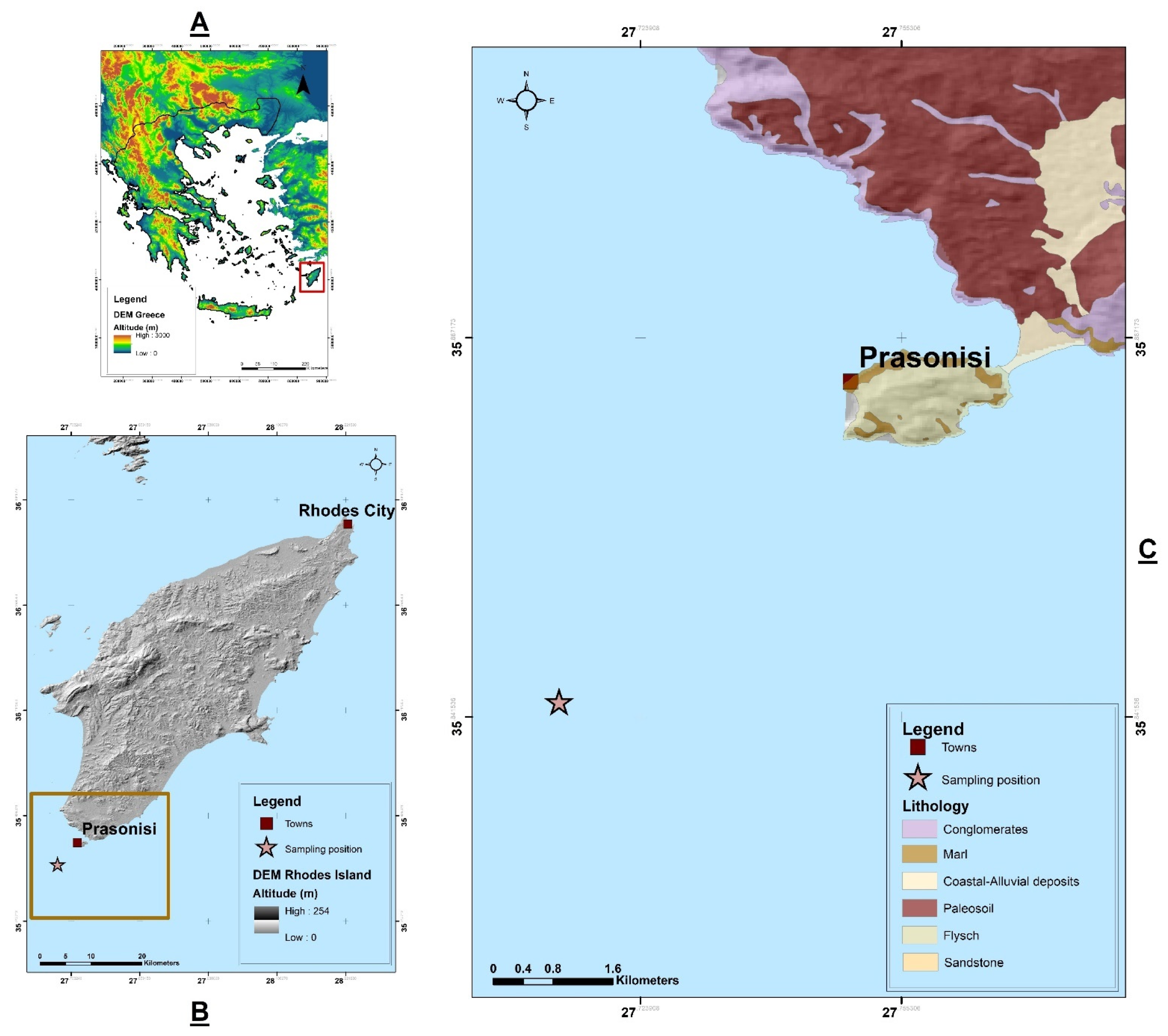
2. The Study Area
3. Materials and Methods
3.1. Used Data
3.2. Extraction of Wave Scenarios
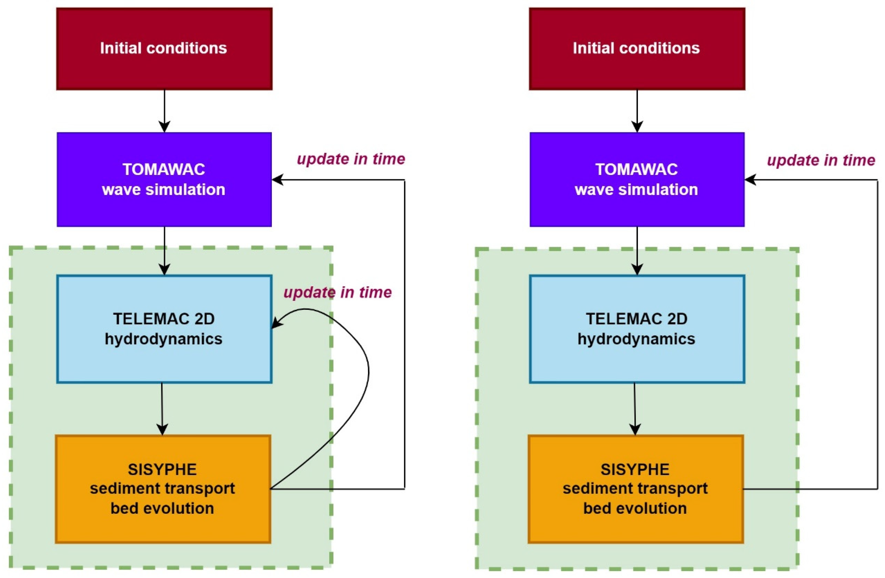
3.3. Numerical Model Setup
3.3.1. Numerical Models, Time, and Sediment Parameters Description
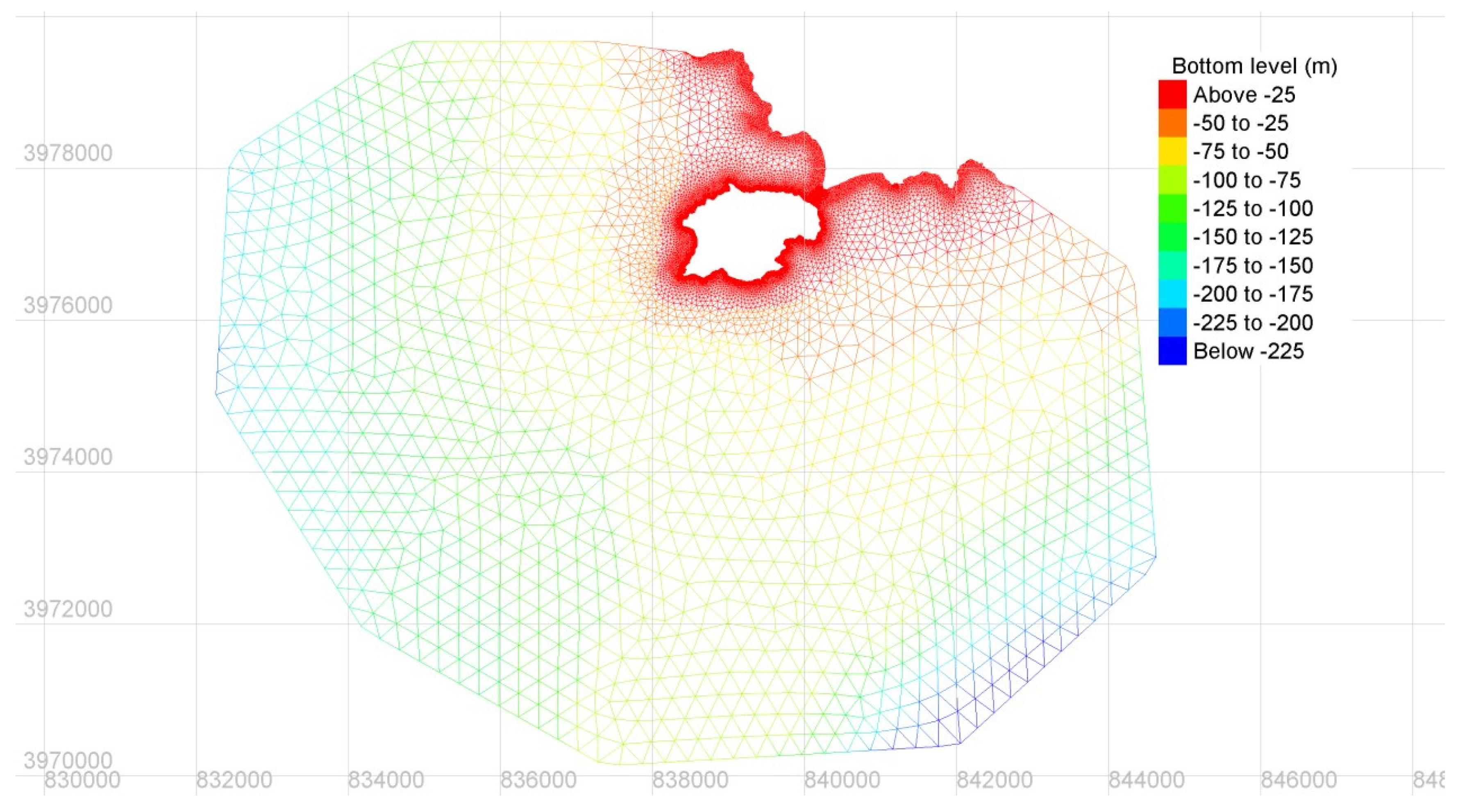
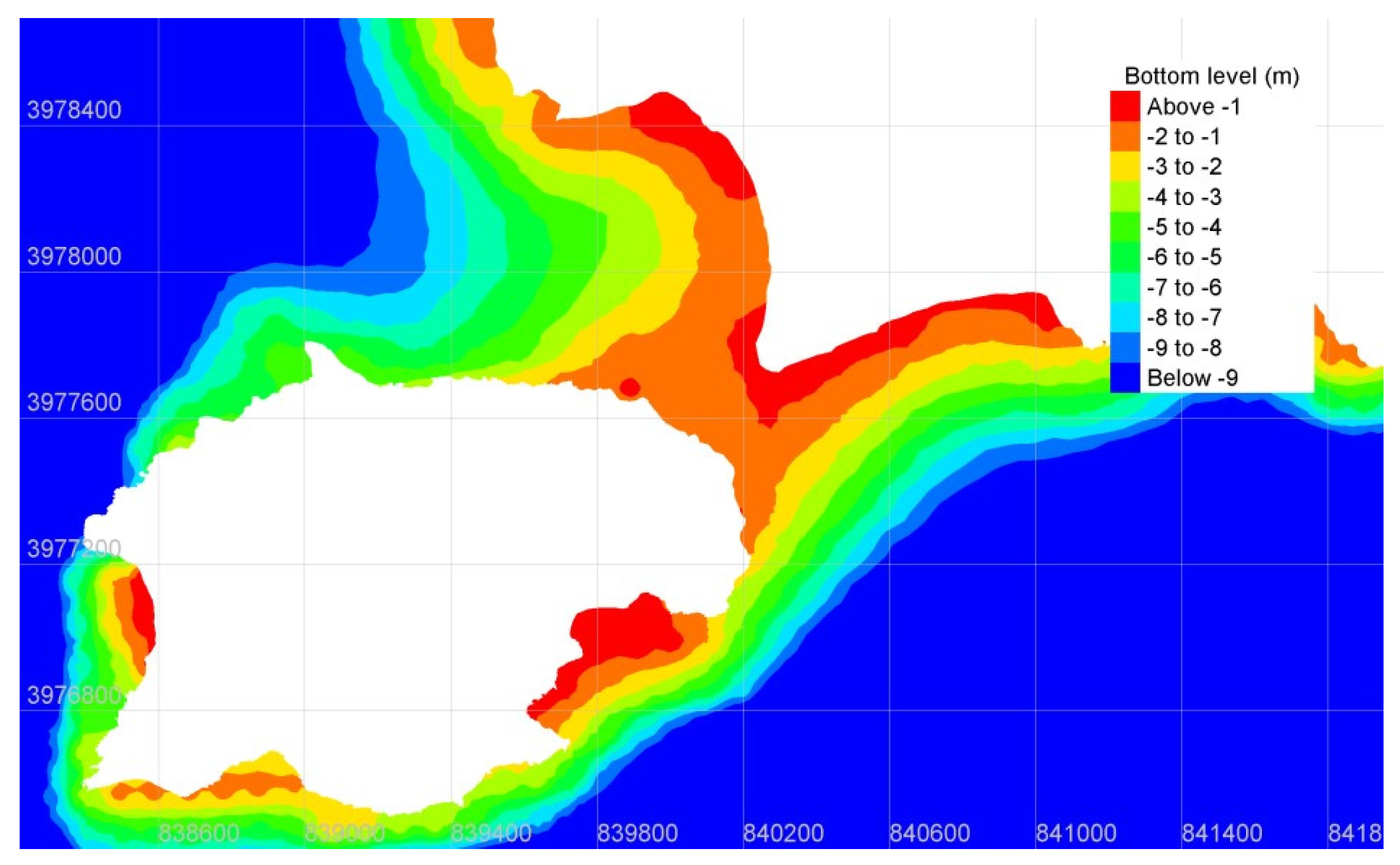
3.3.2. Bathymetry
4. Results
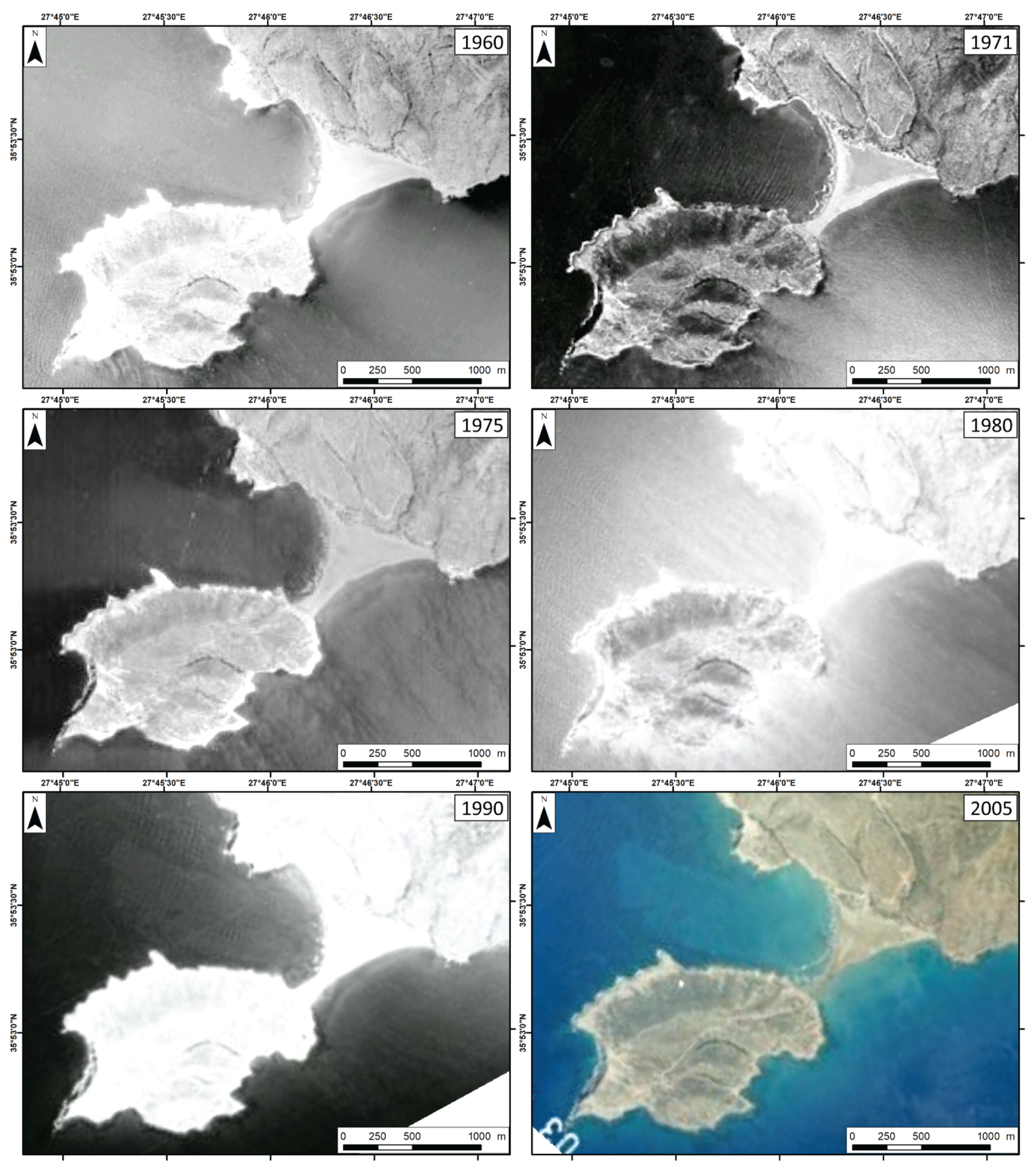
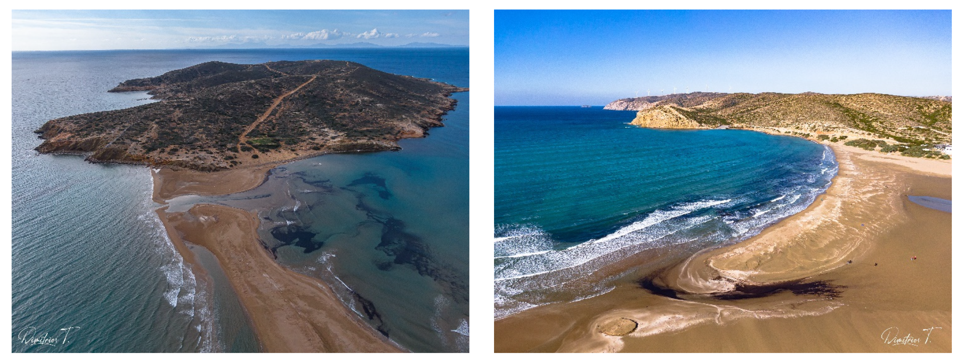
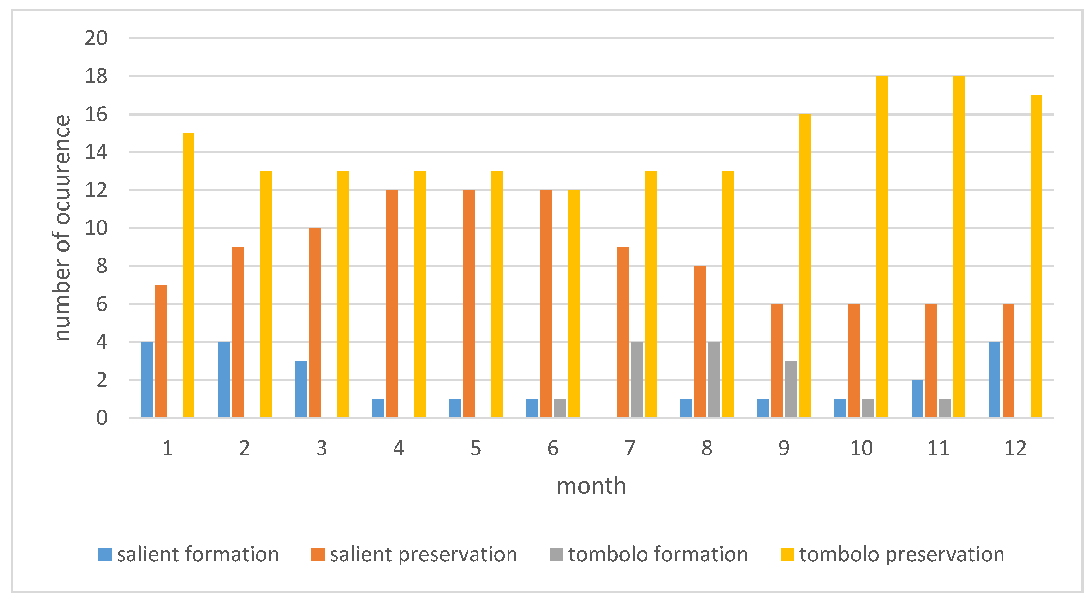
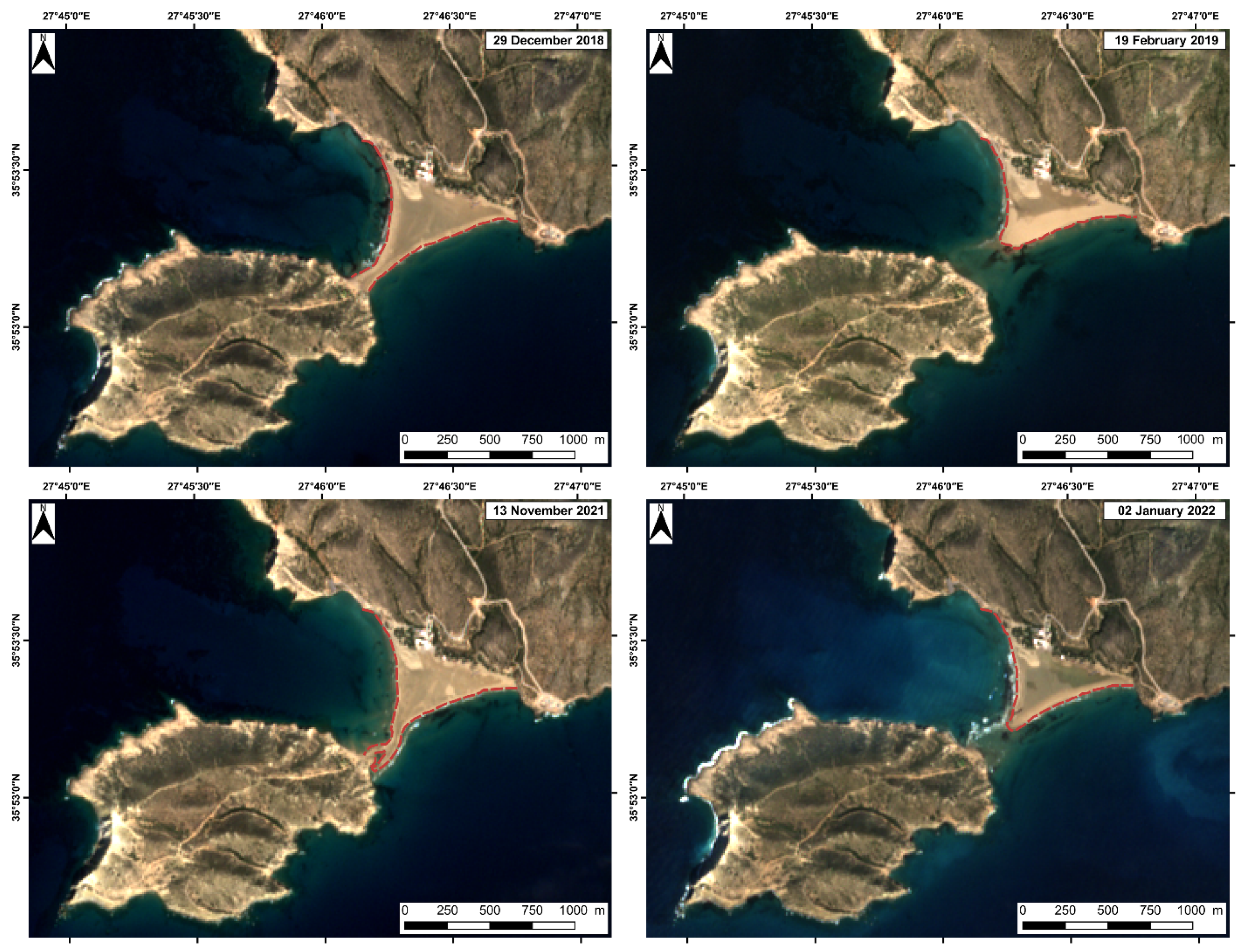
4.1. Investigation of Long-Term Morphological Changes and Seasonality of the Prasonisi Tombolo and Salient Based on Satellite Images
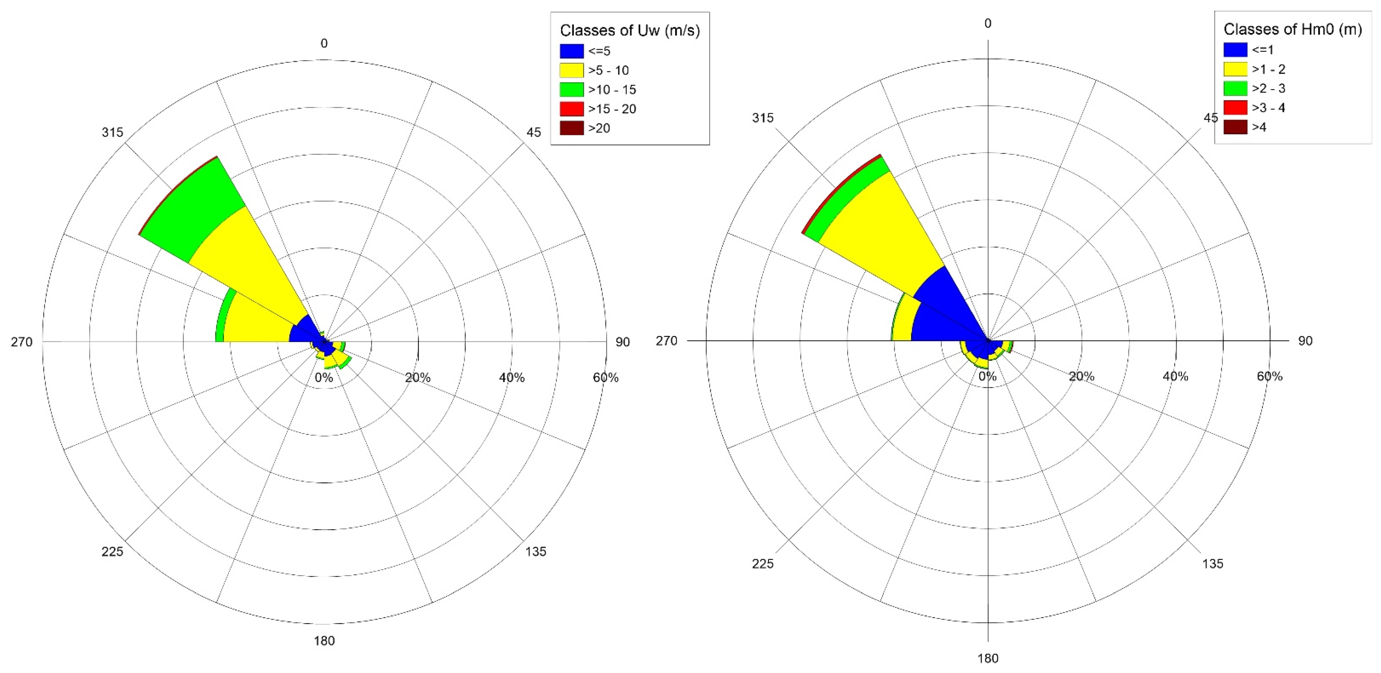
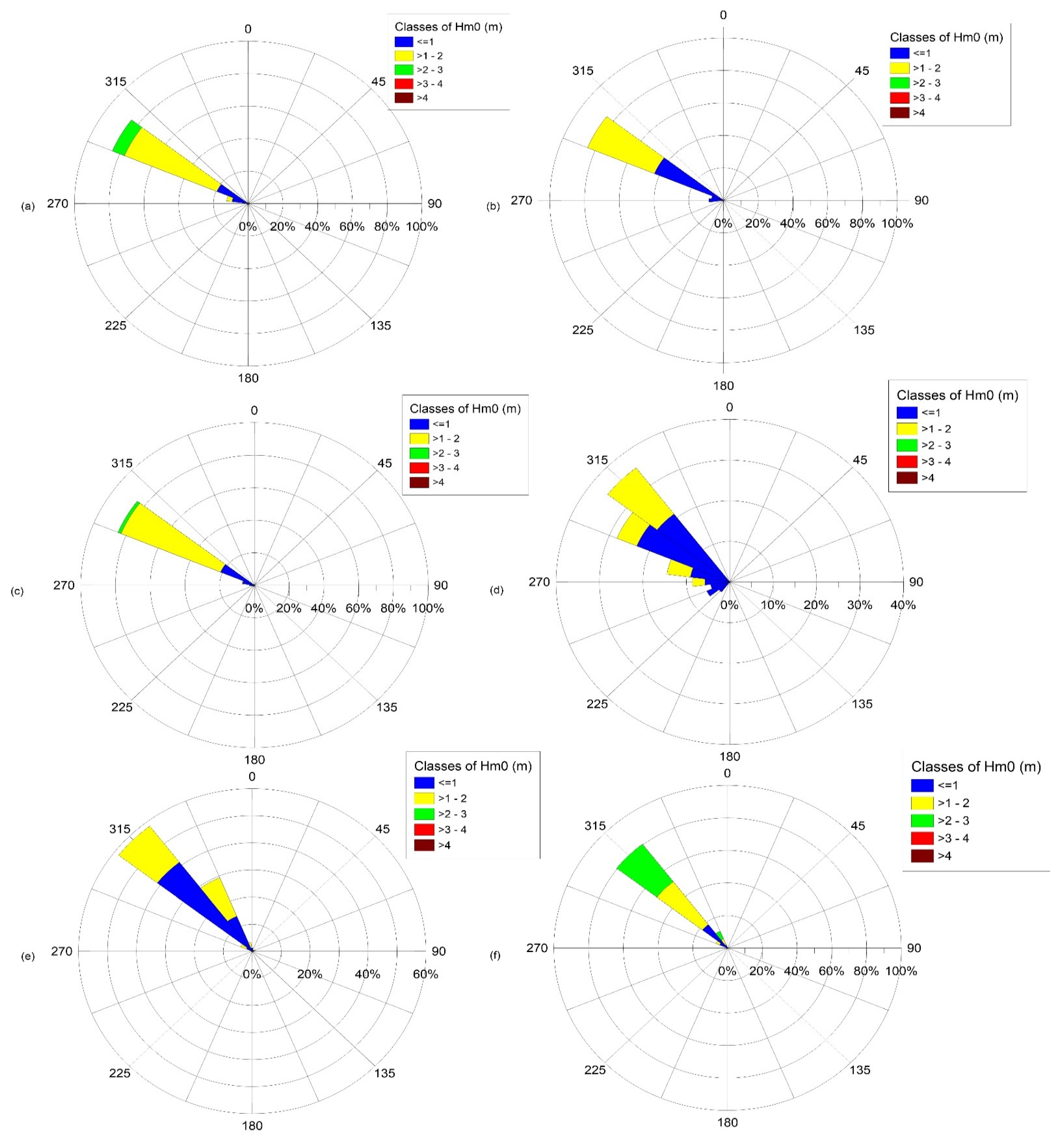
4.2. Long-Term Wave Climate
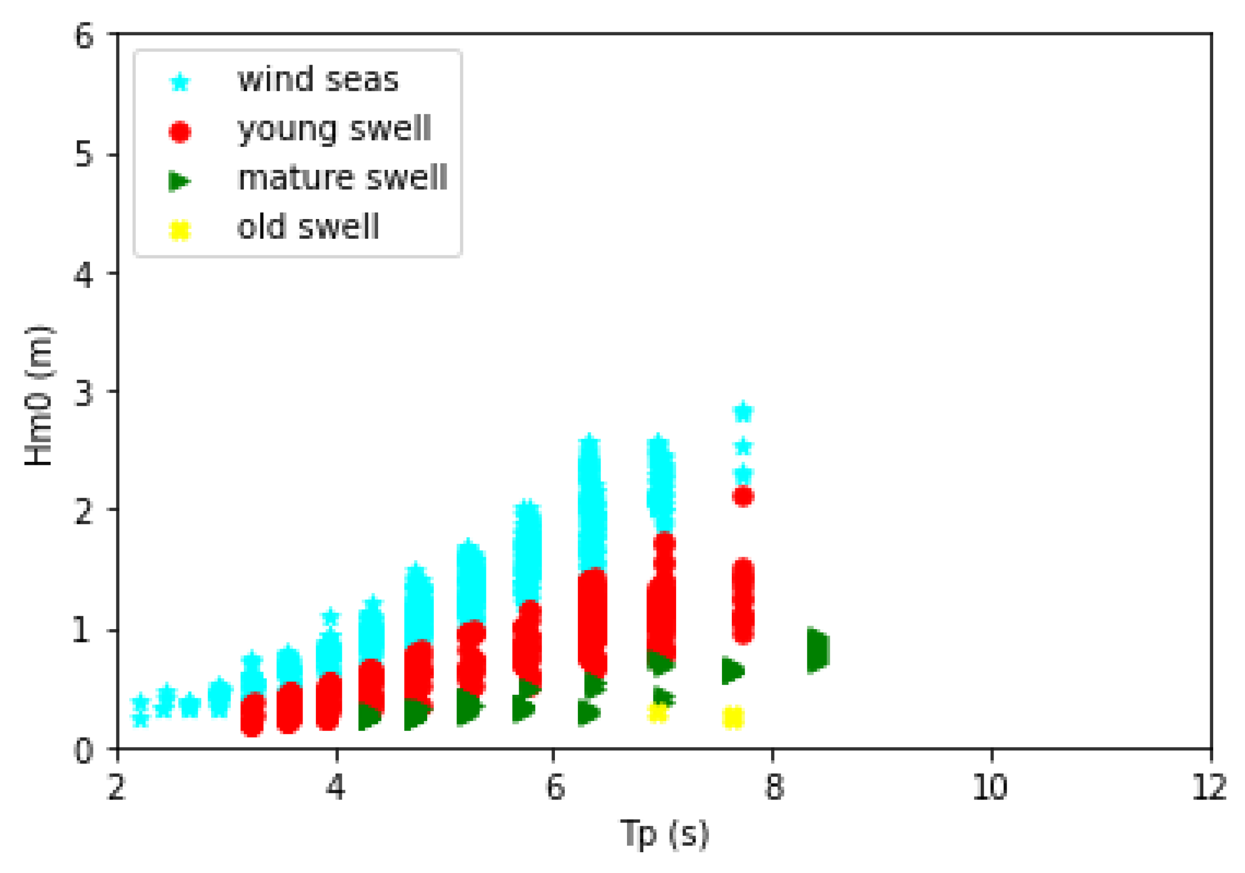
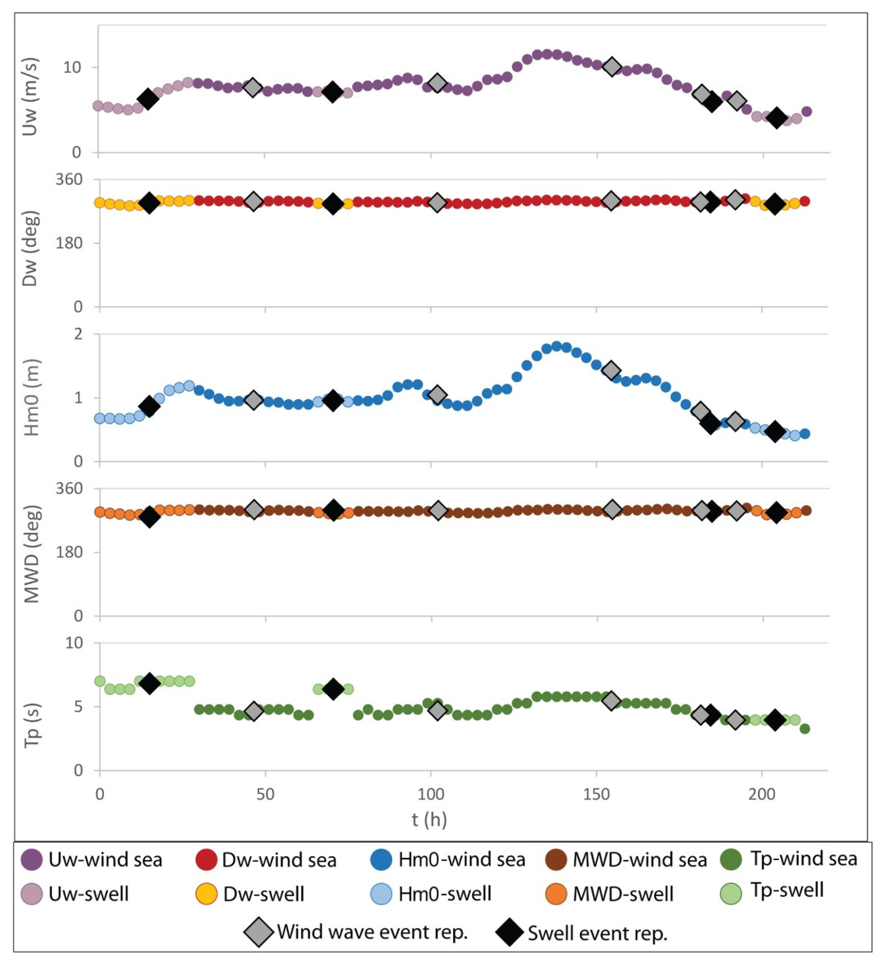
4.3. Extracting Wave Scenarios for the Investigation of the Tombolo and Salient Formation
4.4. Numerical Investigation of the Tombolo and Salient Formation
5. Discussion
6. Conclusions
Supplementary Materials
Author Contributions
Funding
Institutional Review Board Statement
Informed Consent Statement
Data Availability Statement
Acknowledgments
Conflicts of Interest
References
- De Mahiques, M.M. Tombolo. In Encyclopedia of Estuaries. Encyclopedia of Earth Sciences Series; Kennish, M.J., Ed.; Springer: Dordrecht, The Netherland, 2016; pp. 713–714. [Google Scholar]
- Tsiaras, A.-C.; Karambas, T.; Koutsouvela, D. Design of Detached Emerged and Submerged Breakwaters for Coastal Protection: Development and Application of an Advanced Numerical Model. J. Waterw. Port Coastal Ocean Eng. 2020, 146, 04020012. [Google Scholar] [CrossRef]
- Elghandour, A.; Roelvink, D.; Huisman, B.; Reyns, J.; Costas, S.; Nienhuis, J. Reduced Complexity Modeling of Shoreline Response Behind Offshore Breakwaters. Coast. Eng. Proc. 2020, 34, 1. [Google Scholar] [CrossRef]
- Sanderson, P.G.; Eliot, I. Shoreline salients, cuspate forelands and tombolos on the Coast of Western Australia. J. Coast. Res. 1996, 12, 761–773. [Google Scholar]
- Da Fontoura Klein, A.H.; Junior, N.A.; De Menezes, J.T. Shoreline Salients and Tombolos on the Santa Catarina coast (Brazil): Description and analysis of the morphological relationships. J. Coast. Res. 2002, 36, 425–440. [Google Scholar] [CrossRef]
- Specht, C.; Lewicka, O.; Specht, M.; Zblewski, S. Impact of hydrotechnical structures on forming the tombolo oceanographic phenomenon in kołobrzeg and sopot. TransNav 2021, 15, 687–694. [Google Scholar] [CrossRef]
- Shigemura, T.; Takasugi, J.; Komiya, Y. Formation of tombolo at the west coast of Iwo-Jima. Coast. Eng. 1984 1985, 1403–1419. [Google Scholar]
- Suh, K.D.; Hardaway, C.S. Calculation of Tombolo in shoreline numerical model. Proc. Coast. Eng. Conf. 1995, 3, 2653–2667. [Google Scholar] [CrossRef]
- Flinn, D. The role of wave diffraction in the formation of St. Ninian’s Ayre (Tombolo) in Shetland, Scotland. J. Coast. Res. 1997, 13, 202–208. [Google Scholar]
- Pirazzoli, P.A.; Stiros, S.C.; Arnold, M.; Laborel, J.; Laborel-Deguen, F.; Papageorgiou, S. Episodic uplift deduced from Holocene shorelines in the Perachora Peninsula, Corinth area, Greece. Tectonophysics 1994, 229, 201–209. [Google Scholar] [CrossRef]
- Marriner, N.; Goiran, J.P.; Morhange, C. Alexander the Great’s tombolos at Tyre and Alexandria, eastern Mediterranean. Geomorphology 2008, 100, 377–400. [Google Scholar] [CrossRef]
- Stock, F.; Halder, S.; Opitz, S.; Pint, A.; Seren, S.; Ladstätter, S.; Brückner, H. Late Holocene coastline and landscape changes to the west of Ephesus, Turkey. Quat. Int. 2019, 501, 349–363. [Google Scholar] [CrossRef]
- Hansom, J.D. St Ninian’s Tombolo. Coast. Geomorphol. Great Britain. Geol. Conserv. Rev. 2003, 28, 1–5. [Google Scholar]
- Sunamura, T.; Mizuno, O. A study on Depositional Shoreline Forms Behind an Island. Annual Report No. 13; University of Tsukuba: Tsukuba, Japan, 1987. [Google Scholar]
- Ming, D.; Chiew, Y.M. Shoreline Changes behind Detached Breakwater. J. Waterw. Port Coastal Ocean Eng. 2000, 126, 63–70. [Google Scholar] [CrossRef]
- Black, K.P.; Andrews, C.J. Sandy Shoreline Response to Offshore Obstacles Part 1: Salient and Tombolo Geometry and Shape. J. Coast. Res. 2001, SI 29, 82–93. [Google Scholar]
- González, M.; Medina, R. On the application of static equilibrium bay formulations to natural and man-made beaches. Coast. Eng. 2001, 43, 209–225. [Google Scholar] [CrossRef]
- Bricio, L.; Negro, V.; Diez, J.J. Geometric Detached Breakwater Indicators on the Spanish Northeast Coastline. J. Coast. Res. 2008, 245, 1289–1303. [Google Scholar] [CrossRef]
- Van Rijn, L. Design of Hard Coastal Structures Against Erosion. Available online: http://www.leovanrijn-sediment.com/papers/Coastalstructures2013.pdf (accessed on 10 February 2022).
- Clark, J. Coastal Zone Management Handbook; CRC Press/Lewis Publishers: Boca Raton, FL, USA, 1996. [Google Scholar]
- Houston, J.R. The economic value of beaches—A 2013 update. Shore Beach 2013, 81, 3–11. [Google Scholar]
- Mooser, A.; Anfuso, G.; Mestanza, C.; Williams, A. Management Implications for the Most Attractive Scenic Sites along the Andalusia Coast (SW Spain). Sustainability 2018, 10, 1328. [Google Scholar] [CrossRef] [Green Version]
- Ramli, I.R.; Bahar, A.; Samad, W. Beach Tourism Development Strategy in Coastal Area District Tete Bone, South Sulawesi, Indonesia. Int. J. Environ. Agric. Biotechnol. 2019, 4, 1762–1767. [Google Scholar] [CrossRef]
- Hellenic Military Geographical Service. Available online: https://www.gys.gr/index_en.html (accessed on 20 February 2022).
- Lekkas, E.; Papanikolaou, D.; Sakellariou, D. Neotectonic Map of Greece, Rhodes Sheet 1:100,000; National and Kapodistrian University of Athens: Athens, Greece, 2000. [Google Scholar]
- Vandarakis, D.; Panagiotopoulos, I.P.; Loukaidi, V.; Hatiris, G.-A.; Drakopoulou, P.; Kikaki, A.; Gad, F.-K.; Petrakis, S.; Malliouri, D.I.; Chatzinaki, M.; et al. Assessment of the Coastal Vulnerability to the Ongoing Sea Level Rise for the Exquisite Rhodes Island (SE Aegean Sea, Greece). Water 2021, 13, 2169. [Google Scholar] [CrossRef]
- Gad, F.-K.; Chatzinaki, M.; Vandarakis, D.; Kyriakidou, C.; Kapsimalis, V. Assessment of Wave Storm-Induced Flood Vulnerability in Rhodes Island, Greece. Water 2020, 12, 2978. [Google Scholar] [CrossRef]
- Soukissian, T.; Prospathopoulos, A.; Korres, G.; Papadopoulos, A.; Hatzinaki, M.; Kambouridou, M. A new wind and wave atlas of the Hellenic Seas. In Proceedings of the 27th International Conference on Offshore Mechanics and Arctic Engineering, Estoril, Portugal, 15–20 June 2008. [Google Scholar]
- Mutti, E.; Orombelli, G.; Pozzi, R. Geological studies on the Dodecanese Islands (Aegean Sea): IX. Geological map of the Island of Rhodes (Greece); explanatory notes. Ann. Géologiques Pays Helléniques 1970, 22, 79–226. [Google Scholar]
- Korres, G.; Ravdas, M.; Zacharioudaki, A.; Denaxa, D.; Sotiropoulou, M.; Copernicus Monitoring Environment Marine Service (CMEMS). Mediterranean Sea Waves Reanalysis (CMEMS Med-Waves, MedWAM3 system) (Version 1) Set. Available online: https://resources.marine.copernicus.eu/product-detail/MEDSEA_MULTIYEAR_WAV_006_012/INFORMATION (accessed on 15 February 2021).
- Korres, G.; Ravdas, M.; Zacharioudaki, A.; Denaxa, D.; Sotiropoulou, M.; Copernicus Monitoring Environment Marine Service (CMEMS). Mediterranean Sea Waves Analysis and Forecast (CMEMS MED-Waves, MedWAΜ3 system) (Version 1) Set. Available online: https://resources.marine.copernicus.eu/product-detail/MEDSEA_ANALYSISFORECAST_WAV_006_017/INFORMATION (accessed on 15 February 2021).
- Thompson, W.C.; Nelson, A.R.; Sedivy, D.G. Wave Group Anatomy of Ocean Wave Spectra. Proc. Coast. Eng. Conf. 1985, 1, 661–677. [Google Scholar] [CrossRef]
- Silvester, R. Engineering Aspects of Coastal Sediment Movement. J. Waterw. Harb. Div. 1959, 85, 11–40. [Google Scholar] [CrossRef]
- Rashmi, R.; Aboobacker, V.M.; Vethamony, P.; John, M.P. Co-existence of wind seas and swells along the west coast of India during non-monsoon season. Ocean Sci. 2013, 9, 281–292. [Google Scholar] [CrossRef] [Green Version]
- Carter, D.J.T. Prediction of wave height and period for a constant wind velocity using the JONSWAP results. Ocean Eng. 1982, 9, 17–33. [Google Scholar] [CrossRef]
- Kazeminezhad, M.H.; Etemad-Shahidi, A.; Mousavi, S.J. Application of fuzzy inference system in the prediction of wave parameters. Ocean Eng. 2005, 32, 1709–1725. [Google Scholar] [CrossRef]
- United States. Coastal Engineering Manual; U.S. Army Corps of Engineers: Washington, DC, USA, 2006. [Google Scholar]
- Yamartino, R.J. A Comparison of Several “Single-Pass” Estimators of the Standard Deviation of Wind Direction. J. Clim. Appl. Meteorol. 1984, 23, 1362–1366. [Google Scholar] [CrossRef] [Green Version]
- Fisher, N.I. Statistical Analysis of Circular Data; Cambridge University Press: Cambridge, UK, 1995. [Google Scholar]
- Mardia, K.V.; Peter, I.J. Directional Statistics; Wiley Series in Probability and Statistics; Mardia, K.V., Jupp, P.E., Eds.; John Wiley & Sons, Inc.: Hoboken, NJ, USA, 1999; ISBN 9780470316979. [Google Scholar]
- Soukissian, T.H. Probabilistic modeling of directional and linear characteristics of wind and sea states. Ocean Eng. 2014, 91, 91–110. [Google Scholar] [CrossRef]
- Walstra, D.J.R.; Hoekstra, R.; Tonnon, P.K.; Ruessink, B.G. Input reduction for long-term morphodynamic simulations in wave-dominated coastal settings. Coast. Eng. 2013, 77, 57–70. [Google Scholar] [CrossRef]
- Benedet, L.; Dobrochinski, J.P.F.; Walstra, D.J.R.; Klein, A.H.F.; Ranasinghe, R. A morphological modeling study to compare different methods of wave climate schematization and evaluate strategies to reduce erosion losses from a beach nourishment project. Coast. Eng. 2016, 112, 69–86. [Google Scholar] [CrossRef]
- Coles, S.G. An Introduction to Statistical Modeling of Extreme Values; Springer: London, UK, 2001. [Google Scholar]
- Martzikos, N.T.; Prinos, P.E.; Memos, C.D.; Tsoukala, V.K. Statistical analysis of Mediterranean coastal storms. Oceanologia 2021, 63, 133–148. [Google Scholar] [CrossRef]
- Dissanayake, P.; Brown, J.; Wisse, P.; Karunarathna, H. Effects of storm clustering on beach/dune evolution. Mar. Geol. 2015, 370, 63–75. [Google Scholar] [CrossRef]
- Eichentopf, S.; Karunarathna, H.; Alsina, J.M. Morphodynamics of sandy beaches under the influence of storm sequences: Current research status and future needs. Water Sci. Eng. 2019, 12, 221–234. [Google Scholar] [CrossRef]
- Papadimitriou, A.; Panagopoulos, L.; Chondros, M.; Tsoukala, V. A Wave Input-Reduction Method Incorporating Initiation of Sediment Motion. J. Mar. Sci. Eng. 2020, 8, 597. [Google Scholar] [CrossRef]
- Karathanasi, F.E.; Belibassakis, K.A. A cost-effective method for estimating long-term effects of waves on beach erosion with application to Sitia Bay, Crete. Oceanologia 2019, 61, 276–290. [Google Scholar] [CrossRef]
- Benoit, M.; Marcos, F.; Becq, F. Development of a third generation shallow-water wave model with unstructured spatial meshing. In Proceedings of the 25th International Conference on Coastal Engineering, Orlando, FL, USA, 2–6 September 1996; pp. 465–478. [Google Scholar]
- Hervouet, J.-M. Hydrodynamics of Free Surface Flows. Modelling with the Finite Element Method; Wiley: Hoboken, NJ, USA, 2007. [Google Scholar]
- Hasselmann, D.E.; Dunckel, M.; Ewing, J.A. Directional wave spectra observed during JONSWAP 1973. J.Phys. Ocean. 1980, 10, 1264–1280. [Google Scholar] [CrossRef]
- Forristall, G.Z.; Ewans, K.C. Worldwide Measurements of Directional Wave Spreading. J. Atmos. Ocean. Technol. 1998, 15, 440–469. [Google Scholar] [CrossRef]
- Alpers, W. Monte Carlo simulations for studying the relationship between ocean wave and synthetic aperture radar image spectra. J. Geophys. Res. 1983, 88, 1745. [Google Scholar] [CrossRef]
- Ewans, K.C. Directional Spreading in Ocean Swell. In Ocean Wave Measurement and Analysis (2001); American Society of Civil Engineers: Reston, VA, USA, 2002; pp. 517–529. [Google Scholar]
- Soulsby, R. Dynamics of Marine Sands; Thomas Telford: London, UK, 1997. [Google Scholar]
- Rijn, L.C. van Sediment Transport, Part II: Suspended Load Transport. J. Hydraul. Eng. 1984, 110, 1613–1641. [Google Scholar] [CrossRef]
- Celik, I.; Rodi, W. Modeling Suspended Sediment Transport in Nonequilibrium Situations. J. Hydraul. Eng. 1988, 114, 1157–1191. [Google Scholar] [CrossRef]
- Easterbrook, D.T. Surface Processes and Landforms, 2nd ed.; Prentice Hall Inc.: Upper Saddle River, NJ, USA, 1999. [Google Scholar]
- Kamphuis, J.W. Along shore sediment transport rate. J. Waterw. Port Coastal Ocean Eng. 1991, 117, 624–641. [Google Scholar] [CrossRef]
- Guillou, N. Estimating wave energy flux from significant wave height and peak period. Renew. Energy 2020, 155, 1383–1393. [Google Scholar] [CrossRef]
- Bagnold, R. Mechanics of Marine Sedimentation, The Sea. Intersci. Publ. 1963, 3, 507–528. [Google Scholar]
- Komar, P.D. The mechanics of sand transport on beaches. J. Geophys. Res. 1971, 76, 713–721. [Google Scholar] [CrossRef]
- Thornton, E.B. Distribution of sediment transport across the surf zone. Coast. Eng. Proc. 1972, 1, 52. [Google Scholar] [CrossRef] [Green Version]
- Shibayama, T.; Higuchi, A.; Horikawa, K. Sediment transport due to breaking waves. Coast. Eng. Proc. 1986, 1, 111. [Google Scholar] [CrossRef] [Green Version]
- Dally, W.R.; Dean, R.G. Discussion on: Mass flux and underflow in a surf zone. J. Coast. Eng. 1986, 10, 289–299. [Google Scholar] [CrossRef]
- Thornton, E.B.; Guza, R.T. Transformation of wave height distribution. J. Geophys. Res. 1983, 88, 5925. [Google Scholar] [CrossRef] [Green Version]
- LeMehaute, B. On non-saturated breakers and the wave run-up. In Proceedings of the 8th International Conference Coastal Engineering, Tokyo, Japan, 3–5 April 2001; pp. 77–92. [Google Scholar]
- Weggel, R.G. Maximum breaker height. J. Waterw. Harb. Coast Eng Div. 1972, 98, 529–548. [Google Scholar] [CrossRef]
- Owens, E.H. Tombolo. In Beaches and Coastal Geology. Encyclopedia of Earth Sciences Series; Springer: New York, NJ, USA, 1982; pp. 838–839. [Google Scholar]


| s/n | Datasets | From | To | Δt (h) |
|---|---|---|---|---|
| 1 | Wave and Wind Atlas of the Hellenic Seas | 1 January 1995 | 31 December 2004 | 3 |
| 2 | Copernicus-MEDSEA_HINDCAST_WAV_006_012 | 2 February 2006 | 1 January 2020 | 1 |
| 3 | Copernicus-MEDSEA_ANALYSISFORECAST_WAV_006_017 | 2 January 2020 | 2 June 2021 | 1 |
| Start Date | End Date | State of Morphology | Satellite | Symbol |
|---|---|---|---|---|
| [ | ) | |||
| 10 November 1995 | 24 March 1996 | salient formation | Landsat 4-5 TM | 1_sf |
| 24 March 1996 | 28 June 1996 | salient preservation | Landsat 4-5 TM | 2_sp |
| 28 June 1996 | 15 August 1996 | tombolo formation | Landsat 4-5 TM | 3_tf |
| 15 August 1996 | 9 January 1998 | tombolo preservation | Landsat 4-5 TM | 4_tp |
| 9 January 1998 | 30 March 1998 | salient formation | Landsat 4-5 TM | 5_sf |
| 30 March 1998 | 13 August 2001 | salient preservation | Landsat 4-5 TM | 6_sp |
| 13 August 2001 | 22 August 2001 | tombolo formation | Landsat 4-5 TM | 7_tf |
| 22 August 2001 | 9 August 2002 | tombolo preservation | Landsat 4-5 TM | 8_tp |
| 9 August 2002 | 25 June 2003 | salient formation | Landsat 4-5 TM | 9_sf |
| 25 June 2003 | 18 June 2004 | salient preservation | Landsat 4-5 TM | 10_sp |
| 18 June 2004 | 6 September 2004 | tombolo formation | Landsat 4-5 TM | 11_tf |
| 6 September 2004 | 11 December 2004 | tombolo preservation | Landsat 4-5 TM | 12_tp |
| 11 December 2004 | 15 January 2005 | salient formation | Landsat 4-5 TM | 13_sf |
| 15 January 2005 | 7 July 2005 | salient preservation | Landsat 4-5 TM | 14_sp |
| 7 July 2005 | 8 August 2005 | tombolo formation | Landsat 4-5 TM | 15_tf |
| 8 August 2005 | 4 February 2010 | tombolo preservation | Landsat 4-5 TM | 16_tp |
| 4 February 2010 | 11 February 2010 | salient formation | Landsat 4-5 TM | 17_sf |
| 11 February 2010 | 12 June 2010 | salient preservation | Landsat 4-5 TM | 18_sp |
| 12 June 2010 | 28 June 2010 | tombolo formation | Landsat 4-5 TM | 19_tf |
| 28 June 2010 | 19 November 2010 | tombolo preservation | Landsat 4-5 TM | 20_tp |
| 19 November 2010 | 28 December 2010 | salient formation | Landsat 4-5 TM | 21_sf |
| 28 December 2010 | 12 October 2011 | salient preservation | Landsat 4-5 TM | 22_sp |
| 12 October 2011 | 6 November 2011 | tombolo formation | Landsat 4-5 TM | 23_tf |
| 6 November 2011 | ? | tombolo preservation | Landsat 4-5 TM | 24_tp |
| ? | 19 May 2013 | salient formation | Landsat 8 OLI/TIRS | 25_sf |
| 19 May 2013 | 30 August 2013 | salient preservation | Landsat 8 OLI/TIRS | 26_sp |
| 30 August 2013 | 15 September 2013 | tombolo formation | Landsat 8 OLI/TIRS | 27_tf |
| 15 September 2013 | 4 February 2019 | tombolo preservation | Sentinel-2 L2A | 28_tp |
| 4 February 2019 | 14 February 2019 | salient formation | Sentinel-2 L2A | 29_sf |
| 14 February 2019 | 2 June 2021 | salient preservation | Sentinel-2 L2A | 30_sp |
| 2 June 2021 | 13 November 2021 | tombolo formation | Sentinel-2 L2A | 31_tf |
| 13 November 2021 | 2 January 2022 | tombolo preservation | Sentinel-2 L2A | 32_tp |
| 2 January 2022 | 8 February 2022 | salient formation | Sentinel-2 L2A | 33_sf |
| 8 February 2022 | 7 April 2022 | salient preservation | Sentinel-2 L2A | 34_sp |
| a/a | Hm0 (m) | Tp (s) | MWD of Propagation (deg. from North) | Duration (h) |
|---|---|---|---|---|
| 1 | 1.00 | 4.60 | 120 | 3 |
| 2 | 1.50 | 5.55 | 120 | 3 |
| 3 | 1.00 | 6.40 | 120 | 3 |
| 4 | 1.00 | 7.80 | 120 | 3 |
| 5 | 3.00 | 7.70 | 130 | 3 |
| 6 | 4.70 | 9.15 | 310 | 3 |
| Wave Scenario a/a | Hm0 (m) | Tp (s) | MWD (deg) | Total Sand Accretion (m3) | Total Sand Loss (m3) |
|---|---|---|---|---|---|
| 1 | 1.00 | 4.60 | 120 | 1207 | 0 |
| 2 | 1.50 | 5.55 | 120 | 25,154 | 0 |
| 3 | 1.00 | 6.40 | 120 | 4567 | 0 |
| 4 | 1.00 | 7.80 | 120 | 7191 | 0 |
| Wave Scenario a/a | Hm0 (m) | Tp (s) | MWD (deg) | Total Sand Accretion (m3) | Total Sand Loss (m3) (2) |
|---|---|---|---|---|---|
| 5 | 3.00 | 7.70 | 130 | 3.00 | 281,013 |
| 6 | 4.70 | 9.15 | 310 | 4.70 | 194,724 |
Publisher’s Note: MDPI stays neutral with regard to jurisdictional claims in published maps and institutional affiliations. |
© 2022 by the authors. Licensee MDPI, Basel, Switzerland. This article is an open access article distributed under the terms and conditions of the Creative Commons Attribution (CC BY) license (https://creativecommons.org/licenses/by/4.0/).
Share and Cite
Malliouri, D.I.; Petrakis, S.; Vandarakis, D.; Kikaki, K.; Hatiris, G.-A.; Gad, F.-K.; Panagiotopoulos, I.P.; Kapsimalis, V. The Role of Sea State to the Morphological Changes of Prasonisi Tombolo, Rhodes Island, Greece. Water 2022, 14, 2016. https://doi.org/10.3390/w14132016
Malliouri DI, Petrakis S, Vandarakis D, Kikaki K, Hatiris G-A, Gad F-K, Panagiotopoulos IP, Kapsimalis V. The Role of Sea State to the Morphological Changes of Prasonisi Tombolo, Rhodes Island, Greece. Water. 2022; 14(13):2016. https://doi.org/10.3390/w14132016
Chicago/Turabian StyleMalliouri, Dimitra I., Stelios Petrakis, Dimitris Vandarakis, Katerina Kikaki, Georgios-Angelos Hatiris, Fragkiska-Karmela Gad, Ioannis P. Panagiotopoulos, and Vasilios Kapsimalis. 2022. "The Role of Sea State to the Morphological Changes of Prasonisi Tombolo, Rhodes Island, Greece" Water 14, no. 13: 2016. https://doi.org/10.3390/w14132016