
Prediction of the Discharge Flow in a Small Hydropower Station without Hydrological Data Based on SWAT Model

School of Electrical Engineering, Guangxi University, Nanning 530004, China
*
Author to whom correspondence should be addressed.
Water 2022, 14(13), 2011; https://doi.org/10.3390/w14132011
Submission received: 13 May 2022
/
Revised: 14 June 2022
/
Accepted: 20 June 2022
/
Published: 23 June 2022
(This article belongs to the Special Issue Hydrology of Small Catchments and Reservoir Sedimentation)
Abstract
:The availability of hydrological data for small hydropower plants is an important prerequisite for reservoir scheduling, reservoir flood control and integrated water resources. To address the problem of a lack of hydrological data in small hydropower plants, this paper proposes a method to predict the power generation flow of small hydropower stations without hydrological data using the Soil and Water Assessment Tool model (SWAT) when the traditional data-driven methods cannot study the problem of power generation flow prediction in small hydropower stations well. The method can use gridded meteorological data as the input of the model to solve the problem of small hydropower stations without meteorological data. The problem that small hydropower plants without hydrological data cannot calibrate the hydrological model is solved by calculating the generation flow through the output of small hydropower station and by using the similarity analysis method to migrate the generation flow of similar small hydropower stations. The model was tested in a watershed in southwest China to demonstrate the effectiveness of the proposed method. The results show that the coefficient of determination between the predicted and measured values of small hydropower stations without information is about 0.84, which achieves a better prediction.
1. Introduction
Facing the new changes in the global energy pattern, vigorously developing clean low-carbon energy is the main direction of energy development. From a global perspective, as a clean renewable energy source, small hydropower (a single hydropower station with an installed capacity of less than 50,000 kW) resources is almost the main force of hydropower resources and it is the most important support and guarantee to achieve the goal of "carbon emissions peak and carbon neutrality" and realize the energy transformation of human society [1,2]. There has been a great deal of research and many excellent methods proposed in the field of streamflow prediction, for example Costa Silva, D. F. et al. [3] proposed an integrated Long Short-Term Memory (LSTM) model that tested streamflow prediction for five scenarios using runoff and rainfall data. Hu, Y. et al. [4] used flow data from a hydrological station and precipitation data from 11 surrounding rainfall stations to build an LSTM model for flow prediction in small rivers. Zaini, N et al. [5] used ten years of historical rainfall, river flow data and various meteorological data to construct support vector machine (SVM) models and their coupled models with particle swarm optimization (PSO) models for daily river flow prediction. However, most of these studies are carried out under the premise of having complete or relatively complete hydrological information. According to the research, most of the small hydropower plants are located in remote areas and the equipment and facilities of the power stations are relatively backward and they have been in the situation of no hydrological information, which will seriously affect the optimal scheduling of small hydropower groups and the flood prevention of power stations [6]. How to make scientific and efficient prediction of small hydropower generation flow without hydrological information, so as to improve the safety and comprehensive water resource utilization of small hydropower, has been an urgent problem.
Prediction of ungauged watersheds has always been one of the most important and challenging problems. In the field of hydrology, construction of hydrological models and regionalization based on hydrological similarity are often used to carry out studies of uninformed watersheds [7,8,9]. Hydrological models commonly used for flow simulation are: Variable Infiltration Capacity Macroscale Hydrologic Model (VIC) [10,11,12], Soil and Water Assessment Tool model [13,14,15,16], Hydrologiska Byråns Vattenbalansavdelning model (HBV) [17,18], etc. Among them, the SWAT model is a distributed hydrological model with strong physical mechanism [19], the model can be simulated from three different time scales of year, month and day for continuous long-term simulation, and can use geographic information data and remote sensing data to establish a hydrological model in ungauged watershed. The SWAT model is one of the most widely used basin hydrology models in the world and can be found in various research areas [20]. For example, Narula, K. et al. [21] used the SWAT model to simulate and calibrate streamflow in two montane forested watersheds. Kanishka, G. et al. [22] proposed a method to combine watershed classification with regionalization using a dimensionality reduction technique and used the SWAT model for streamflow prediction. Using the method of constructing hydrological models to physically solve the problem of predicting power generation flow in small hydropower plants without hydrological information can effectively avoid the traditional data-driven inability to obtain data for prediction.
Against the above background, the main objective of this study is to carry out research on the problem of small hydropower flow prediction without hydrological information based on the SWAT hydrological model and to solve the current problems of small hydropower (especially private small hydropower plants) due to the serious lack of hydrological information, which makes flow prediction difficult and scheduling work difficult, by combining similarity analysis, cluster analysis and construction of basin hydrological model. This study can provide a novel and reliable idea for the future development of flow prediction of small hydropower plants without hydrological data and provide data support for the unified scheduling and management of small hydropower and monitoring of ecological flow in the future.
2. Materials and Methods
2.1. Research Area
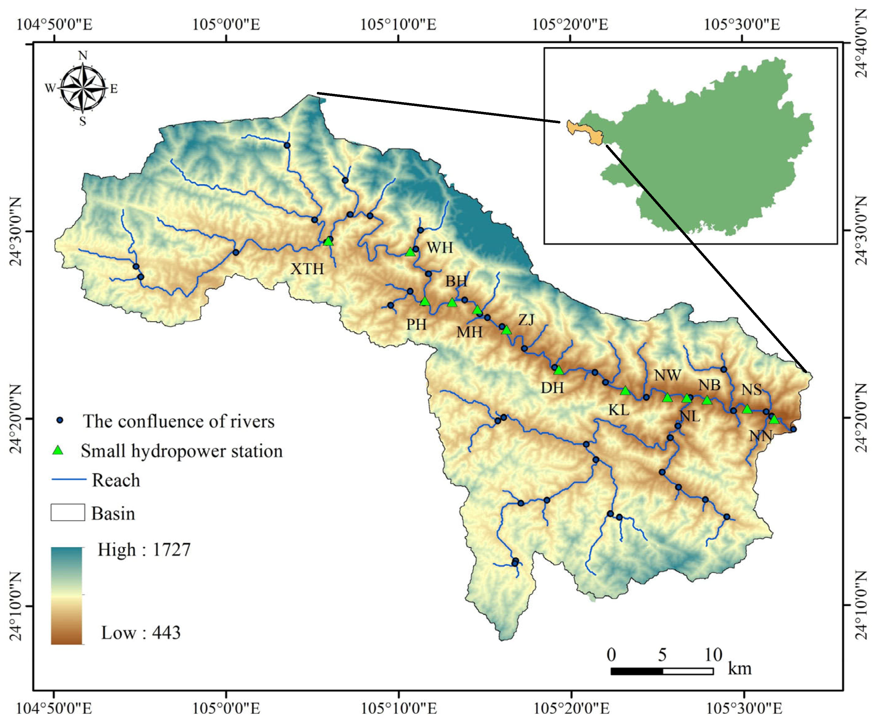
This paper chooses a section of watershed which flows through a county in southwest China, including XTH, WH, PH, BH, MH, ZJ, DH, KL, NW, NL, NB, NS and NN small hydropower stations. Its location information is shown in Figure 1.
2.2. Data Sources
The data used in this paper to build the model mainly include geospatial data, meteorological data and basic information data of small hydropower stations. Geospatial data mainly include DEM digital elevation map, soil distribution map and land use distribution map of the study area. Land use data come from the Institute of Geographical Sciences and Natural Resources Research, Chinese Academy of Sciences. The soil data come from Harmonized World Soil Database. The meteorological data adopt The China Meteorological Assimilation Driving Datasets for the SWAT model (CMADS) [23], which mainly includes rainfall, solar radiation, maximum and minimum temperature, wind speed and relative humidity.
The specific sources and accuracy of the data are shown in Table 1.
2.3. SWAT Model
The watershed hydrological process of the SWAT model can be divided into the land surface part of the water cycle (runoff and slope confluence part) and the water surface part of the water cycle (the river confluence part) [24]. From the model structure, this model belongs to the second type of distributed hydrological model. That is, from each grid unit (or sub-basin), the traditional conceptual model is applied to infer the net rainfall, then the confluence calculation is performed and finally the outlet section flow is obtained. Using the SWAT model to simulate the hydrological cycle of the small hydropower domain can directly output the flow of each small hydropower without hydrological data, which is a new attempt to solve the problem of no data for small hydropower.
In each hydrological response unit (HRU), from the rainfall to the confluence of water, the potential path of the water flow process simulated by SWAT is the process of hydrological simulation calculation by the model. The principle of water balance is the basic principle for the establishment of the SWAT model [25,26], and the formula for calculating the water volume is:
The meanings of the parameters in the formula are shown in Table 2.
The SWAT model uses the CN value method of the SCS model and the Green-Ampt infiltration method to calculate the surface runoff [27]. The calculation equation of the SCS~CN curve is:
where is a daily surface runoff (mm); is daily rainfall (mm); is the initial abstraction which includes surface storage, interception and infiltration prior to runoff (mm); and represents retention parameter (mm).
The hydrological cycle of surface runoff is shown in Figure 2.
2.4. Correlation Analysis
In the preliminary data preparation, both geospatial data and meteorological data are relatively easy to obtain. Because most of the small hydropower stations are located in remote areas with few or no hydrological stations, it is difficult to obtain historical hydrological data. This paper proposes three methods to obtain historical hydrological data to calibrate the model:
(1) Direct method: the runoff data of hydrological station can be obtained directly;
(2) Indirect method: if similar small hydropower stations do not have hydrological data, their output can be used to calculate the discharge flow, and finally the model can be calibrated. The calculation formula of the discharge flow of the hydropower station is:
where refers to the output of small hydropower stations (kW), refers to the efficiency of turbines, the general value is 0.85–0.96, refers to the efficiency of generators, the general value is 0.96–0.98, refers to the generating flow () and refers to the reservoir water head (m).
(3) Similarity method: When there is neither a hydrological station nor a small hydropower station in the basin and there is no historical power output data, the similarity method is selected. First select similar power stations of small hydropower stations without hydrological data through correlation analysis and cluster analysis, and then use the discharge flow of similar power stations or calculate the discharge flow through indirect method to calibrate the model.
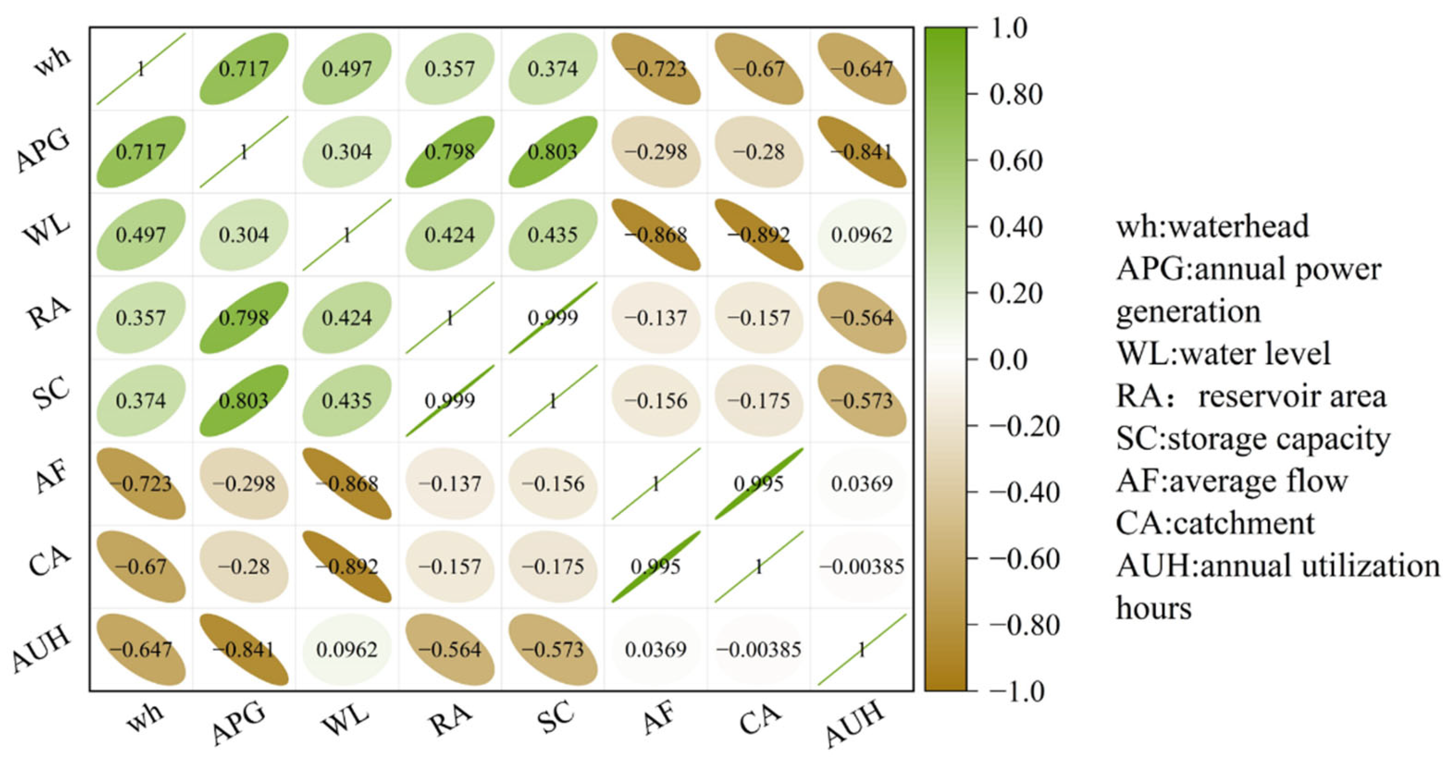
Pearson analysis method [28] is used to screen out the variables with high correlation coefficient with flow among the basic variables of small hydropower stations. The calculation formula of Pearson simple correlation coefficient is as follows:
where represents Pearson correlation coefficient, represents the number of small hydropower stations, and represent two different parameters and and represent average values of parameters.
As shown in Figure 3, the correlation analysis results show that the discharge of the power plant has a high correlation with the area of rainfall collection above the dam site, the normal water level and the waterhead.
2.5. Clustering Analysis
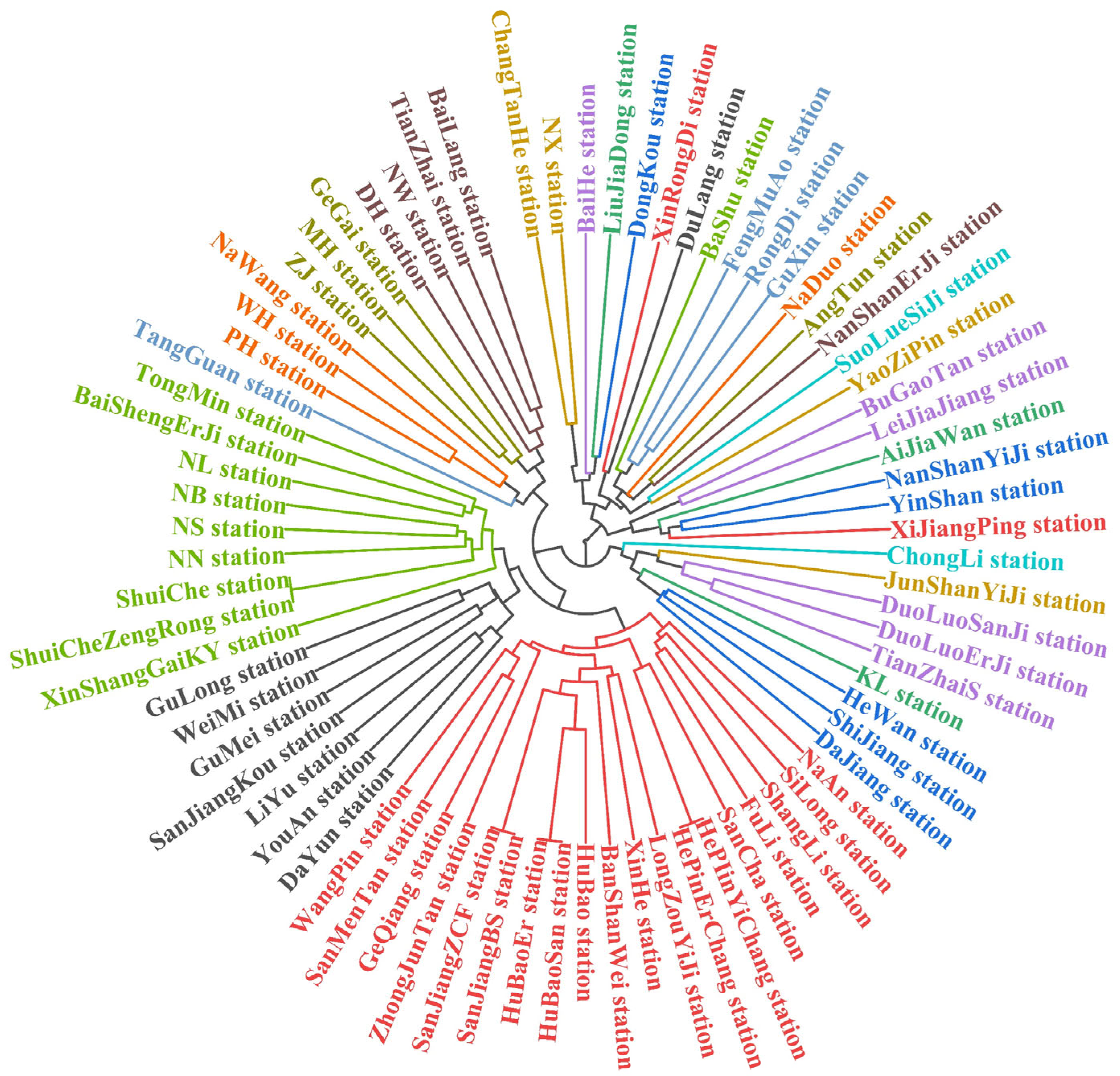
After the correlation analysis, the system clustering method was used to analyze and study the four parameters of the average flow, the catchment area on the dam, the normal water level and the water head of the 78 small hydropower stations around the basin and to find the similar power stations of the small hydropower stations without hydrological data. The discharge flow or output of similar power stations to determine the discharge flow of small hydropower stations without hydrological data. Similar power stations of each small water point after clustering are shown in Figure 4.
2.6. Construction of SWAT Model
2.6.1. Watershed Delineation
After splicing multiple DEMs in the study area, load them into ArcSWAT and set the DEM attributes, then generate a river network, add reservoir nodes to facilitate the selection of reservoir positioning in the later stage and then specify the total outlet of the watershed and divide the sub-basins. Finally, calculate the parameters of the sub-basin and add reservoirs.
2.6.2. Land Use
Land use data have an important influence on the model results and are indispensable data for building a model. It directly affects the process of rainfall on the land surface. To establish the land-use-type index table, it is necessary to reclassify the land use data, as shown in Table 3.
2.6.3. Soil Data
Soil data are also some of the very important data in the SWAT model. The quality of soil data will have an important impact on the model results. The physical properties of soil determine the movement of water and air in the soil profile and play an important role in water cycle in the HRU.
When building a soil database, first crop and project the downloaded soil raster, then reclassify the soil data and set the values of various variables in the usersoil database. Then, use the SPAW software to calculate the soil wet density, effective water holding capacity, saturated hydraulic conductivity and other parameters, and finally calculate the soil infiltration rate according to the average soil particle size layer by layer, divide the hydrological grouping and establish the soil-type index table.
2.6.4. HRU Analysis
After the sub-basin division is completed, the hydrological response unit is divided. The main steps are to define land use data, soil data and slope data and import the index table of land use and soil corresponding data. Then, define the hydrological response unit and set the land use threshold, soil-type threshold and slope threshold. Finally, divide the study area into 108 hydrological response units.
2.6.5. Weather Data Definition
This paper uses the CMADS dataset. First select the meteorological stations in the research basin, then construct the index table of meteorological data and then import data into the model. After the model is built, set the time step and warm-up period and run the model to output the results.
3. Results and Discussion
3.1. Parameter Sensitivity Analysis
After running the SWAT model, calibration and sensitivity analysis of the model parameters is required. On the basis of referring to a large number of literatures, nine parameters that have a greater impact on runoff are selected. The relative significance of the parameter is represented by the t-Stat value, and the larger the absolute value of t-Stat, the more sensitive the parameter is. The p-Value represents the probability value of P corresponding to the t-test value, and the closer the value is to 0, the more sensitive the parameter is [19].
In this paper, the continuous uncertainty rate method (SUFI2) is used to determine the parameters. After 2000 iterations of the model, the parameter sensitivity and optimal parameter values are shown in Table 4. The CN2 parameter has the highest sensitivity, followed by the CANMX parameter.
3.2. SWAT Model Calibration and Results Analysis
Calibration of hydrological models in the absence of hydrological information is one of the difficulties that make it possible to carry out studies of small hydropower stations without hydrological information. Without the calibration of the hydrological model, the training effect will be very different from the measured value. The SWAT-CUP tool is one of the effective ways to calibrate the SWAT model and this tool is suitable to support decision makers in conceptualizing sustainable watershed management, allowing decision makers to better calibrate the model [29,30].
This manuscript proposes the direct method, the indirect method and the similarity method to obtain the measured value. This paper adopts the similarity method to obtain the discharge flow to calibrate the model. The objective function for parameter calibration uses Nash–Sutcliffe efficiency coefficient (NSE) and coefficients of determination [31].
(1) NSE: Nash–Sutcliffe efficiency coefficient is an important index to evaluate the accuracy of model simulation:
where is the simulated value of discharge flow from small hydropower station; represents the measured value of discharge flow; is the mean of the measured discharge flow; and is the length of the measured discharge flow.
(2) represents the determinant coefficient and evaluates the correlation between the model simulation value and the measured value:
where is the simulated value of the discharge flow; represents the measured value of the discharge flow; is the mean of the measured discharge flow; is the mean of the simulated discharge flow; and is the length of the measured discharge flow.
Among the 13 small hydropower stations in the research basin, the MH station and the NW station are selected as the sites for the calibration of the SWAT model. After 2000 calibrations (as shown in Table 5 and Figure 5), the discharge flow of the MH small hydropower station has the NSE value of 0.74, the determination coefficient value of 0.84 and the NSE value of the NW small hydropower station is 0.73. The value of the coefficient is 0.78.
When the value of NSE is 1, it means that the simulation results are very perfect and the measured and simulated values are exactly equal. When the value of NSE is between 0.6 and 1, it means that the simulation results are better. When the value of NSE is less than 0, the simulation results are poor. The coefficient of determination represents the correlation between the measured value and the simulated value. The closer the value is to 1, the better the result. It can be seen that the verification results of the two small hydropower stations are good and the accuracy is high.
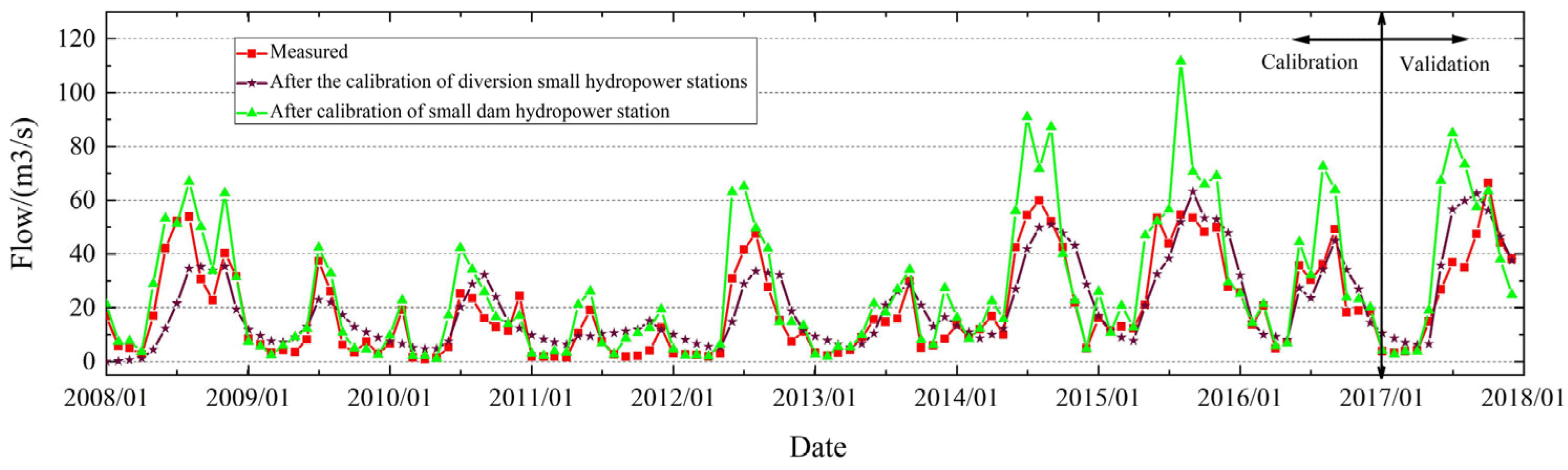
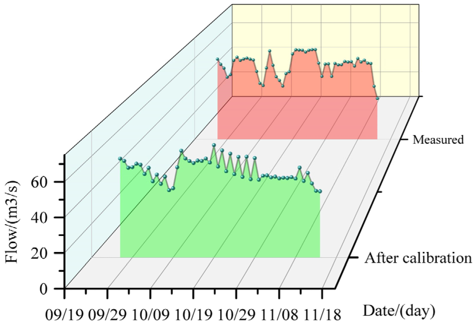
The NB station is chosen as the validation site for no hydrological data. After calibrating the SWAT model, we can directly get the flow rate of NB small hydropower station by setting the river points in advance. Figure 6 and Figure 7 show the test situation of the monthly and daily scale of the discharge flow of NB small hydropower station. It can be seen that before the calibration of the SWAT model, the simulated value is lower than the actual value and the results improved significantly after calibration.
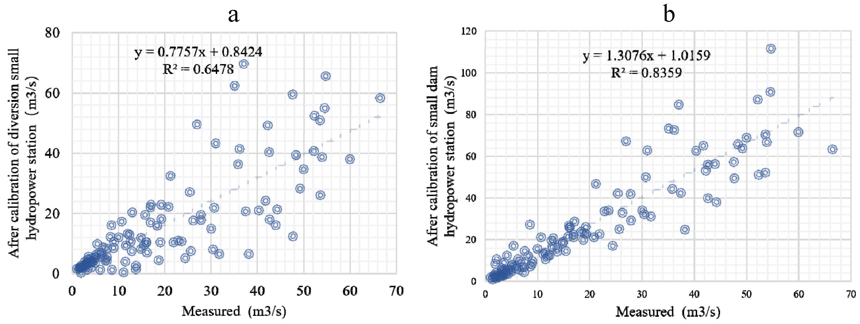
Small hydropower can be divided into dam type, diversion type and hybrid type. In order to conduct a more comprehensive study, this paper conducts an analysis of two cases of NB small hydropower station with and without reservoirs. According to the research, the flow curve of small hydropower station without reservoirs will be smoother and similar to the flow curve of natural rivers. As shown in the red-brown curve in Figure 6, because there is no artificial regulation of the reservoir, this curve is smoother and less accurate, with a correlation coefficient of only about 0.65 in Figure 8. On the contrary, as shown in the green curve in Figure 6, this curve is closer to the measured value and more volatile, with a correlation coefficient of about 0.83 in Figure 8. It is obvious that the NB small hydropower station without hydrological data in this study has a reservoir.
3.3. Uncertainty Analysis
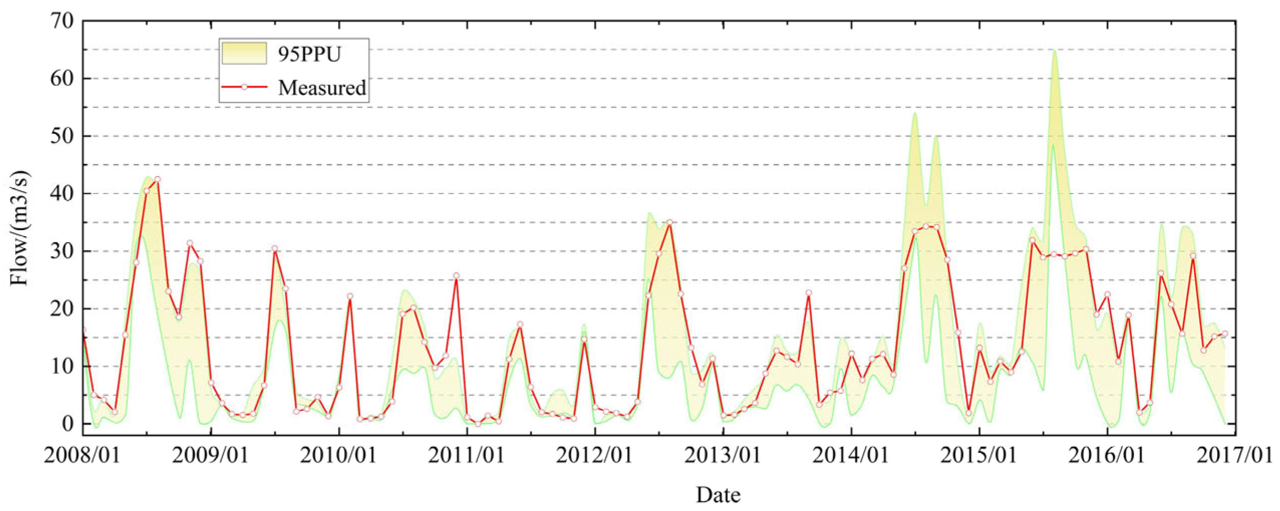
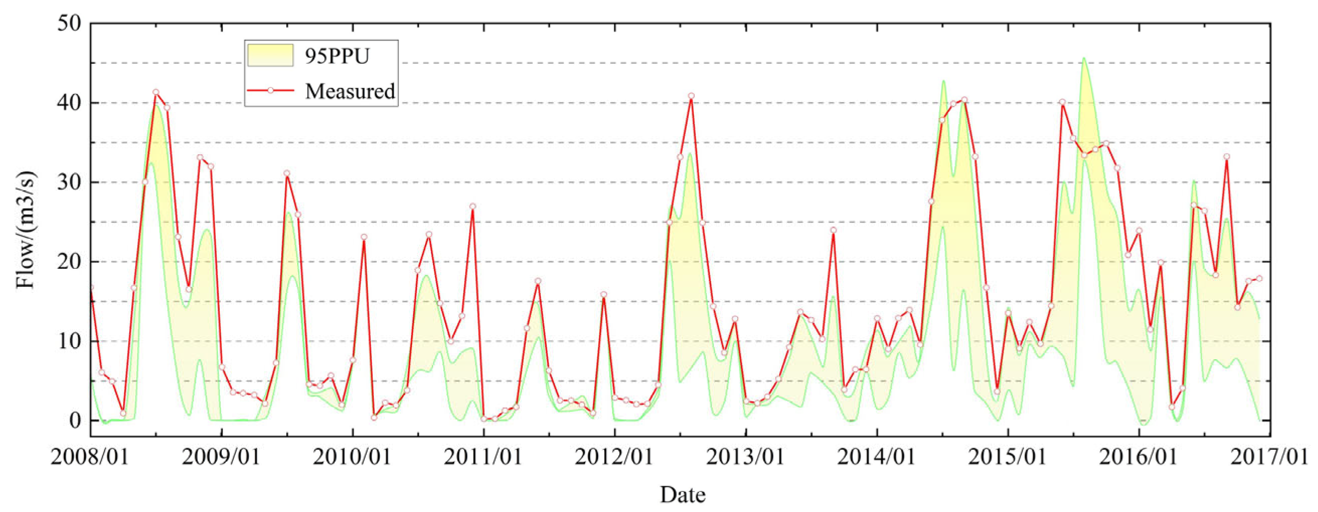
Use 95% confidence intervals to study the effect of model parameter uncertainty on the results. Table 6 shows the two uncertainty indicators of the model in the calibration process. The value of p-factor parameter for MH small hydropower station is 0.3 and r-factor parameter is 0.55. The value of p-factor parameter for NW small hydropower station is 0.68 and r-factor parameter is 0.75.
The p-factor value indicates the proportion of the measured value within the 95% confidence interval of the simulated value. The larger the p-factor value is, the greater the uncertainty of the parameter contributes to the uncertainty of the simulation result, and the value of r-factor is generally less than 1, which means the simulation result is better. The 95% confidence intervals for these two small hydropower stations are shown in Figure 9 and Figure 10.
4. Conclusions and Recommendations
In this paper, the SWAT model is used to predict the power generation flow of small hydropower plants without hydrological information, which innovatively solves the problem of small hydropower plants without hydrological information that makes it impossible to carry out flow prediction and other work; a correlation analysis and cluster analysis are used to classify 78 small hydropower plants, and three methods are proposed to calibrate the model; and a detailed analysis of small hydropower plants without information with and without reservoirs is also carried out. The specific findings of the study are as follows.
The results of the correlation analysis and cluster analysis of 78 small hydropower stations showed that the closer the station to the no-information small hydropower station, the stronger the correlation. After the calibration of the model, the NSE values of MH and NW small hydropower stations were 0.74 and 0.73, and the coefficients of determination were 0.84 and 0.78. It can be seen that the SWAT model has good applicability in the study basin. The results of the sensitivity analysis on the parameters of the model show that the CN2 parameter has the greatest influence on the accuracy of the model. The results of the uncertainty analysis on the parameters of the model show that the larger yellow area in the plots, as shown in Figure 9 and Figure 10, indicates that the parameters of the model have a greater influence on the uncertainty of the prediction results.
The main objective of the research in this paper is to carry out the prediction of power generation flow of small hydropower plants without hydrological information. The monthly power generation flow prediction for small hydropower plants in NB has been better achieved to achieve the daily power generation flow prediction. Additionally, the prediction results are analyzed from two cases with and without reservoirs, and the prediction accuracy is expressed by the decision coefficient, which is 0.64 and 0.83.
Most of the small hydropower stations are in remote areas, where neither hydrological nor meteorological information is available, so the daily generation flow prediction accuracy of this study is low. The problem of missing meteorological data for small hydropower stations can be solved in the future by using correlation methods to migrate meteorological data from large hydropower stations located in the same large basin using transfer learning methods. Similarly, a hydrological model can be established in the watershed where the large hydropower stations are located first, and the model parameters for the watershed where the small hydropower stations are located can be determined using a regionalization approach.
Author Contributions
Conceptualization, S.X. and Y.Z.; methodology, S.X. and Y.Z.; software, S.X.; validation, S.X., Y.Z.; formal analysis, S.X.; investigation, S.X. and Y.Z.; resources, Y.Z.; data curation, S.X.; writing—original draft preparation, S.X.; writing—review and editing, S.X. and Y.Z.; visualization, S.X. and Y.Z.; supervision, Y.Z.; project administration, Y.Z.; funding acquisition, Y.Z. All authors have read and agreed to the published version of the manuscript.
Funding
Guangxi Special Fund for Innovation-Driven Development (AA19254034).
Institutional Review Board Statement
Not applicable.
Informed Consent Statement
Not applicable.
Data Availability Statement
The data presented in this study are available on request from X.S.
Acknowledgments
Many thanks to the editors and reviewers for their valuable comments.
Conflicts of Interest
The authors declare no conflict of interest.
References
- Ugwu, C.O.; Ozor, P.A.; Mbohwa, C. Small hydropower as a source of clean and local energy in Nigeria: Prospects and challenges. Fuel Commun. 2022, 10, 100046. [Google Scholar] [CrossRef]
- Paish, O. Small hydro power: Technology and current status. Renew. Sustain. Energy Rev. 2002, 6, 537–556. [Google Scholar] [CrossRef]
- Costa Silva, D.F.; Galvão Filho, A.R.; Carvalho, R.V.; de Souza, L.; Ribeiro, F.; Coelho, C.J. Water Flow Forecasting Based on River Tributaries Using Long Short-Term Memory Ensemble Model. Energies 2021, 14, 7707. [Google Scholar] [CrossRef]
- Hu, Y.; Yan, L.; Hang, T.; Feng, J. Stream-Flow Forecasting of Small Rivers Based on LSTM. arXiv 2020, arXiv:2001.05681v1. [Google Scholar]
- Zaini, N.; Malek, M.A.; Yusoff, M.; Mardi, N.H.; Norhisham, S. Daily River Flow Forecasting with Hybrid Support Vector Machine—Particle Swarm Optimization. IOP Conf. Ser. Earth Environ. Sci. 2018, 140, 012035. [Google Scholar] [CrossRef]
- Jimeno-Sáez, P.; Senent-Aparicio, J.; Pérez-Sánchez, J.; Pulido-Velazquez, D. A Comparison of SWAT and ANN Models for Daily Runoff Simulation in Different Climatic Zones of Peninsular Spain. Water 2018, 10, 192. [Google Scholar] [CrossRef] [Green Version]
- Razavi, T.; Coulibaly, P. Improving streamflow estimation in ungauged basins using a multi-modelling approach. Hydrol. Sci. J. 2016, 61, 2668–2679. [Google Scholar] [CrossRef] [Green Version]
- Horlacher, H.-B.; Cullmann, J.; Awulachew, S.B.; Saliha, A.H. Estimation of flow in ungauged catchments by coupling a hydrological model and neural networks: Case study. Hydrol. Res. 2011, 42, 386–400. [Google Scholar] [CrossRef]
- Wang, H.; Cao, L.; Feng, R. Hydrological Similarity-Based Parameter Regionalization under Different Climate and Underlying Surfaces in Ungauged Basins. Water 2021, 13, 2508. [Google Scholar] [CrossRef]
- Zhu, B.; Huang, Y.; Zhang, Z.; Kong, R.; Tian, J.; Zhou, Y.; Chen, S.; Duan, Z. Evaluation of TMPA Satellite Precipitation in Driving VIC Hydrological Model over the Upper Yangtze River Basin. Water 2020, 12, 3230. [Google Scholar] [CrossRef]
- Scheidegger, J.M.; Jackson, C.R.; Muddu, S.; Tomer, S.K.; Filgueira, R. Integration of 2D Lateral Groundwater Flow into the Variable Infiltration Capacity (VIC) Model and Effects on Simulated Fluxes for Different Grid Resolutions and Aquifer Diffusivities. Water 2021, 13, 663. [Google Scholar] [CrossRef]
- Zhong, W.; Guo, J.; Chen, L.; Zhou, J.; Zhang, J.; Wang, D. Future hydropower generation prediction of large-scale reservoirs in the upper Yangtze River basin under climate change. J. Hydrol. 2020, 588, 125013. [Google Scholar] [CrossRef]
- Koycegiz, C.; Buyukyildiz, M. Calibration of SWAT and Two Data-Driven Models for a Data-Scarce Mountainous Headwater in Semi-Arid Konya Closed Basin. Water 2019, 11, 147. [Google Scholar] [CrossRef] [Green Version]
- Abbaspour, K.C.; Vaghefi, S.A.; Yang, H.; Srinivasan, R. Global soil, landuse, evapotranspiration, historical and future weather databases for SWAT Applications. Sci. Data 2019, 6, 263. [Google Scholar] [CrossRef] [Green Version]
- Jayakrishnan, R.; Srinivasan, R.; Santhi, C.; Arnold, J.G. Advances in the application of the SWAT model for water resources management. Hydrol. Process. 2005, 19, 749–762. [Google Scholar] [CrossRef]
- Geng, X.; Zhang, C.; Zhang, F.; Chen, Z.; Nie, Z.; Liu, M. Hydrological Modeling of Karst Watershed Containing Subterranean River Using a Modified SWAT Model: A Case Study of the Daotian River Basin, Southwest China. Water 2021, 13, 3552. [Google Scholar] [CrossRef]
- Simonov, Y.A.; Semenova, N.K.; Khristoforov, A.V. Short-Range Streamflow Forecasting of the Kama River Based on the HBV Model Application. Russ. Meteorol. Hydrol. 2021, 46, 388–395. [Google Scholar] [CrossRef]
- Shi, W.; Li, L.; Xia, J.; Gippel, C.J. A hydrological model modified for application to flood forecasting in medium and small-scale catchments. Arab. J. Geosci. 2016, 9, 296. [Google Scholar] [CrossRef]
- Arnold, J.G.; Moriasi, D.N.; Gassman, P.W.; Abbaspour, K.C.; White, M.J.; Srinivasan, R.; Santhi, C.; Harmel, R.D.; Griensven, A.V.; Liew, M.; et al. SWAT: Model Use, Calibration, and Validation. Trans. ASABE 2012, 55, 1491–1508. [Google Scholar] [CrossRef]
- Gassman, P.W.; Sadeghi, A.M.; Srinivasan, R. Applications of the SWAT Model Special Section: Overview and Insights. J. Environ. Qual. 2014, 43, 1–8. [Google Scholar] [CrossRef]
- Narula, K.; Nischal, S. Hydrological Modelling of Small Gauged and Ungauged Mountainous Watersheds Using SWAT—A Case of Western Ghats in India. J. Water Resour. Prot. 2021, 13, 455–477. [Google Scholar] [CrossRef]
- Kanishka, G.; Eldho, T.I. Streamflow estimation in ungauged basins using watershed classification and regionalization techniques. J. Earth Syst. Sci. 2020, 129, 186. [Google Scholar] [CrossRef]
- Meng, X.; Wang, H.; Lei, X.; Cai, S.; Wu, H.; Ji, X. Hydrological Modeling in the Manas River Basin Using Soil and Water Assessment Tool Driven by CMADS. Teh. Vjesn. Tech. Gaz. 2017, 24, 525–534. [Google Scholar] [CrossRef] [Green Version]
- Tian, J.; Guo, S.; Deng, L.; Yin, J.; Pan, Z.; He, S.; Li, Q. Adaptive optimal allocation of water resources response to future water availability and water demand in the Han River basin, China. Sci. Rep. 2021, 11, 7879. [Google Scholar] [CrossRef] [PubMed]
- Arnold, J.G.; Srinivasan, R.; Muttiah, R.S.; Williams, J.R. Large Area Hydrologic Modeling And Assessment Part I: Model Development1. JAWRA J. Am. Water Resour. Assoc. 1998, 34, 73–89. [Google Scholar] [CrossRef]
- Neitsch, S.L.; Arnold, J.G.; Kiniry, J.R.; Williams, J.R. Soil and Water Assessment Tool Theoretical Documentation Version 2009; Texas Water Resources Institute: College Station, TX, USA, 2011. [Google Scholar]
- Kavian, A.; Golshan, M.; Abdollahi, Z. Flow discharge simulation based on land use change predictions. Environ. Earth Sci. 2017, 76, 588. [Google Scholar] [CrossRef]
- Lee Rodgers, J.; Nicewander, W.A. Thirteen Ways to Look at the Correlation Coefficient. Am. Stat. 1988, 42, 59–66. [Google Scholar] [CrossRef]
- Tudose, N.; Marin, M.; Cheval, S.; Ungurean, C.; Davidescu, S.; Tudose, O.; Alin Lucian, M.; Davidescu, A. SWAT Model Adaptability to a Small Mountainous Forested Watershed in Central Romania. Forests 2021, 12, 860. [Google Scholar] [CrossRef]
- De Souza Dias, V.; da Pereira Luz, M.; Medero, G.M.; Tarley Ferreira Nascimento, D.; de Nunes Oliveira, W.; de Rodrigues Oliveira Merelles, L. Historical Streamflow Series Analysis Applied to Furnas HPP Reservoir Watershed Using the SWAT Model. Water 2018, 10, 458. [Google Scholar] [CrossRef] [Green Version]
- Nash, J.E.; Sutcliffe, J.V. River flow forecasting through conceptual models part I—A discussion of principles. J. Hydrol. 1970, 10, 282–290. [Google Scholar] [CrossRef]
Figure 1.
Location information of the study area.

Figure 2.
Schematic diagram of the hydrological cycle of the SWAT model.

Figure 3.
Correlation analysis of parameters of small hydropower stations.

Figure 4.
Cluster analysis diagram of small hydropower stations.

Figure 5.
Simulation results of discharge flow of MH small hydropower station.

Figure 6.
Comparison diagram of discharge flow of NB small hydropower station.

Figure 7.
Daily discharge flow of NB small hydropower station.

Figure 8.
Correlation between measured and predicted values in both cases without (a) and with (b) reservoirs.
Figure 8.
Correlation between measured and predicted values in both cases without (a) and with (b) reservoirs.

Figure 9.
The 95% confidence interval diagram of MH hydropower station.

Figure 10.
The 95% confidence interval diagram of NW hydropower station.


Table 1.
Data source and accuracy of the study area.
| Data | Source | Accuracy |
|---|---|---|
| DEM | Geospatial Data | 30 m × 30 m |
| land use | CAS | 1 km |
| Land cover | HWSD | 1 km |
| Meteorological data | CMADS | Month/day |
Table 2.
The meaning of each parameter of the water balance formula.
| Parameter | Meaning | Unit |
|---|---|---|
| the final soil water content | mm | |
| the initial soil water content | mm | |
| daily rainfall | mm | |
| daily evapotranspiration | mm | |
| daily surface runoff | mm | |
| daily percolation | mm | |
| daily lateral flow | mm |
Table 3.
Statistical table of land use reclassification.
| Name and Code | Area (Hectare) | Ratio (%) |
|---|---|---|
| Forest land (FRST) | 57,803.52 | 37.24 |
| Cultivated land (AGRL) | 78,128.10 | 50.34 |
| Grassland (PAST) | 18,865.81 | 12.16 |
| Residential land (URBN) | 268.25 | 0.17 |
| Waters (WATR) | 132.46 | 0.09 |
Table 4.
Parameter sensitivity analysis and optimal parameter value.
| Parameter | Meaning | Initial Range | Modification Method | Optimal Parameter | p-Value | t-Stat |
|---|---|---|---|---|---|---|
| CN2 | Initial SCS runoff curve number for moisture condition II | 35–98 | v | 96.24 | 0 | 27.73 |
| CANMX | Maximum canopy storage | 0–100 | v | 98.40 | 0 | 3.86 |
| SQL_AWC | Available water capacity of the soil layer | 0–1 | r | 0.02 | 0.37 | 0.88 |
| ESCO | Soil evaporation compensation factor | 0–1 | v | 0.72 | 0.57 | 0.56 |
| REVAPMN | Threshold depth of water in the shallow aquifer for “revap” or percolation to the deep aquifer to occur | 0–500 | v | 253.51 | 0.61 | 0.50 |
| ALPHA_BF | Base flow alpha factor | 0–1 | v | 0.52 | 0.28 | −1.07 |
| EPCO | Plant uptake compensation factor | 0–1 | v | 0.18 | 0.21 | −1.24 |
| GWQMN | Threshold depth of water in the shallow aquifer required for return flow to occur | 0–4500 | v | 3139.44 | 0.16 | −1.40 |
| GW_REVAP | Ground water “revap” coefficient | 0.02–0.2 | r | 0.09 | 0.05 | −1.90 |
Table 5.
Evaluation index of model.
| Station | NSE | |
|---|---|---|
| MH | 0.74 | 0.84 |
| NW | 0.73 | 0.78 |
Table 6.
Uncertainty analysis results.
| Station | p-Factor | r-Factor |
|---|---|---|
| MH | 0.30 | 0.55 |
| NW | 0.68 | 0.75 |
Publisher’s Note: MDPI stays neutral with regard to jurisdictional claims in published maps and institutional affiliations. |
© 2022 by the authors. Licensee MDPI, Basel, Switzerland. This article is an open access article distributed under the terms and conditions of the Creative Commons Attribution (CC BY) license (https://creativecommons.org/licenses/by/4.0/).
Share and Cite
MDPI and ACS Style
Xie, S.; Zhu, Y. Prediction of the Discharge Flow in a Small Hydropower Station without Hydrological Data Based on SWAT Model. Water 2022, 14, 2011. https://doi.org/10.3390/w14132011
AMA Style
Xie S, Zhu Y. Prediction of the Discharge Flow in a Small Hydropower Station without Hydrological Data Based on SWAT Model. Water. 2022; 14(13):2011. https://doi.org/10.3390/w14132011
Chicago/Turabian StyleXie, Shenghuo, and Yun Zhu. 2022. "Prediction of the Discharge Flow in a Small Hydropower Station without Hydrological Data Based on SWAT Model" Water 14, no. 13: 2011. https://doi.org/10.3390/w14132011
Note that from the first issue of 2016, this journal uses article numbers instead of page numbers. See further details here.